1
Habplan User Manual
NCASI Statistics and Model Development Group
∗
Version 3 February 16, 2006
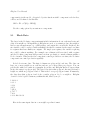
Abstract
Habplan is a landscape management and harvest scheduling program. Habplan
allows you to build an objective function from the supplied components that show up
as checkboxes on the main Habplan form. Habplan was designed to deal with spatial
objectives, but can also be used for harvest scheduling where there are no spatial or
adjacency issues. Habplan selects from management regimes that the user indicates
are allowable for each polygon (stand). Any polygon may have from 1 to hundreds of
allowed regimes.
Habplan was declared to be at version 3 in early 2005 after the addition of several
new features. Habplan now has the ability to write out MPS files for input to a Linear
Program solver. It is also possible to create management units. Polygons that are
∗
NCASI: http://ncasi.uml.edu/
1
Habplan User Manual
placed in the same unit must be assigned the same management regime. Another new
feature enables linking of Flow components. This allows a user to control some key
variables for multiple Flows by making adjustments on a single Flow edit form. Version
3 of Habplan is backward compatible with version 2. This means that anything you
did with version 2 will still work, and you can ignore the new features without penalty.
2
Habplan User Manual
1
Contents
1
Introduction
6
2
Habplan Distribution Policy
8
3
Installing the Program
9
4
Known Bugs
10
5
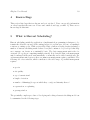
What is Harvest Scheduling?
10
6
5.1
Modelling the Harvest Scheduling Problem . . . . . . . . . . . . . . . . . . .
11
5.2
Solving the Harvest Scheduling Problem . . . . . . . . . . . . . . . . . . . .
12
Main Habplan Menu
6.1
7
Management Units . . . . . . . . . . . . . . . . . . . . . . . . . . . . . . . .
Flow Component
14
15
7.1
Linked Flows . . . . . . . . . . . . . . . . . . . . . . . . . . . . . . . . . . .
16
7.2
Flow Data . . . . . . . . . . . . . . . . . . . . . . . . . . . . . . . . . . . .
17
7.2.1
8
13
Flow Data for PreCut Stands: Spatial Issues . . . . . . . . . . . . . .
19
7.3
Flow Form . . . . . . . . . . . . . . . . . . . . . . . . . . . . . . . . . . . .
20
7.4
Flow Summary . . . . . . . . . . . . . . . . . . . . . . . . . . . . . . . . . .
22
CCFlow Component
24
Habplan User Manual
9
2
8.1
CCFlow Data
. . . . . . . . . . . . . . . . . . . . . . . . . . . . . . . . . .
24
8.2
CCFlow Form . . . . . . . . . . . . . . . . . . . . . . . . . . . . . . . . . .
25
Blocksize Component
26
9.1
Block Data . . . . . . . . . . . . . . . . . . . . . . . . . . . . . . . . . . . .
27
9.2
BlockForm . . . . . . . . . . . . . . . . . . . . . . . . . . . . . . . . . . . .
28
9.3
Block Graphs
31
. . . . . . . . . . . . . . . . . . . . . . . . . . . . . . . . . .
10 Biological Type I Component
10.1 Biological Type I Data
31
. . . . . . . . . . . . . . . . . . . . . . . . . . . . .
33
10.2 Biological Type I Form . . . . . . . . . . . . . . . . . . . . . . . . . . . . .
34
11 Biological Type II Component
36
11.1 Biological Type II Data . . . . . . . . . . . . . . . . . . . . . . . . . . . . .
36
11.2 Biological Type II Form
37
. . . . . . . . . . . . . . . . . . . . . . . . . . . .
12 Spatial Model Component
38
12.1 Spatial Model Data . . . . . . . . . . . . . . . . . . . . . . . . . . . . . . .
40
12.2 Spatial Model Form . . . . . . . . . . . . . . . . . . . . . . . . . . . . . . .
40
13 Comments on Preparing Input Data
41
13.1 Habplan project files . . . . . . . . . . . . . . . . . . . . . . . . . . . . . . .
42
13.1.1 The general section . . . . . . . . . . . . . . . . . . . . . . . . . . . .
43
Habplan User Manual
3
13.1.2 The components section . . . . . . . . . . . . . . . . . . . . . . . . .
44
13.1.3 The bestschedule section . . . . . . . . . . . . . . . . . . . . . . . . .
44
13.1.4 The output section . . . . . . . . . . . . . . . . . . . . . . . . . . . .
44
13.1.5 The gis section . . . . . . . . . . . . . . . . . . . . . . . . . . . . . .
45
13.1.6 The schedule section . . . . . . . . . . . . . . . . . . . . . . . . . . .
45
14 Habplan Output to Files
14.1 Automatic output when schedules are saved for import . . . . . . . . . . . .
47
48
15 Habplan Graphs
48
16 Habplan GIS Viewer
49
16.1 Interactive Regime Editing . . . . . . . . . . . . . . . . . . . . . . . . . . . .
53
17 Definition of a Block
54
18 Fitness Function
56
19 Objective Function Weights
58
20 Linear Programming
59
20.1 LP Formulation . . . . . . . . . . . . . . . . . . . . . . . . . . . . . . . . .
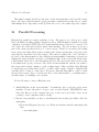
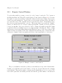
21 Parallel Processing
21.1 Remote Control Window . . . . . . . . . . . . . . . . . . . . . . . . . . . .
62
66
68
Habplan User Manual
4
22 Porting to Other Computers
69
23 User Customization
71
24 Future Directions
72
Habplan User Manual
5
List of Figures
1
Example of Flow Data for Precut Stands . . . . . . . . . . . . . . . . . . . .
20
2
Example of a flow graph . . . . . . . . . . . . . . . . . . . . . . . . . . . . .
23
3
Example of a block graph - not all blocks within specified min and max values 32
4
Example of a block graph - all blocks within specified min and max values .
33
5
Example of spatial model form . . . . . . . . . . . . . . . . . . . . . . . . . .
39
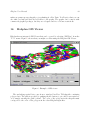
6
Example of GIS viewer . . . . . . . . . . . . . . . . . . . . . . . . . . . . . .
49
7
Example of regime color table . . . . . . . . . . . . . . . . . . . . . . . . . .
50
8
Example of polygon color table . . . . . . . . . . . . . . . . . . . . . . . . .
51
9
Regime Editor . . . . . . . . . . . . . . . . . . . . . . . . . . . . . . . . . . .
53
10
Example of best schedule controls . . . . . . . . . . . . . . . . . . . . . . . .
57
11
Example of LP MPS Generator window . . . . . . . . . . . . . . . . . . . . .
59
12
Example of MPS Config form for entire planning period . . . . . . . . . . . .
60
13
Example of MPS Config form for select years . . . . . . . . . . . . . . . . . .
61
14
Example of Run LP Solver window . . . . . . . . . . . . . . . . . . . . . . .
62
15
Example of an LP Tableau . . . . . . . . . . . . . . . . . . . . . . . . . . . .
63
16
Example of remote control window . . . . . . . . . . . . . . . . . . . . . . .
68
Habplan User Manual
1
6
Introduction
Habplan selects from management regimes that the user indicates are allowable for each
polygon (stand). Any polygon may have from 1 to hundreds of allowed regimes. A regime
encompasses everything that will be done to that polygon over the planning period. Regimes
can therefore be multi-period, i.e. have multiple years where actions and outputs will occur.
Habplan can handle plans involving thousands of polygons and regimes over long planning
horizons. The limits depend only on the size of your computer.
Habplan uses a simulation approach based on the Metropolis Algorithm. It does not
use simulated annealing or genetic algorithms, but is closely related. Habplan is a random
(feasible) schedule generator. It keeps running and generating alterations to the previous
schedule for as long as you like. As the Metropolis iterations proceed, objective function
weights are adaptively determined. This enables Habplan to meet the user’s goals relative
to each component in the objective function. For example, the user specifies whether Flows
should be level, decreasing, or increasing as well as how much year-to-year deviation is
allowed in the flow. The user can also specify minimum and maximum blocksizes along
with green-up windows. Flow and Blocksize are just 2 of the objective function components.
Other components are described below.
Habplan should run under any operating system that has a Java Virtual Machine, which
includes, Windows , Solaris, Linux, and Macs. Installation is easy.
To run the program, you get started by opening a form (from the edit menu) for an
objective function component that you’re interested in. Fill it out and then check the box
on the main Habplan form. This will cause habplan to read the component’s data. Assuming
the data are OK, you are ready to work on filling out another component form, or to press
start to initiate the scheduling algorithm. Use the save option in the File menu so you don’t
have to fill the forms out again. Note that the SUSPEND button suspends the run at the
end of the current iteration, and it can be continued where it left off by pressing the START
button. STOP will stop the run and a subsequent START begins with a new random starting
schedule.
Information about objective function components is given in more detail further along,
but here’s a quick overview of currently available components:
1. F=Flow: You can have as many of these as you want. A Flow component controls
the flow of some output associated with each management option or regime. You
configure Habplan to show the components you want by selecting ”config” under the
Habplan User Manual
7
”Options” menu. After you enter the component (with the checkbox) you can open
an associated graph from the Graph menu. Flow components can also have sub-Flow
components and sub-Flows can have their own sub-Flows. Sub-Flow components might
represent districts and lower level sub-Flows might be watersheds within a district.
Flow components also support thresholding around a target value.
(a) C=ClearCut Flow: This component must be associated with a parent Flow component. Thus, you can have the first flow component (F1) and an associated
clearcut Flow component C1(1). You can have as many of these components as
you want by using the config option. This component reads a file that provides
the size of the polygon. It allows you to keep an even number of acres under certain options. The option doesn’t have to be clear cutting. Also, the variable read
in doesn’t have to be acres. After you enter the component (with the checkbox),
you can open an associated graph from the Graph menu.
(b) BK=BlockSize: This component controls blocksizes associated with the outputs
from a parent Flow component. The first BK associated with F1 is BK1(1). You
can have as many of these components as you want. BK components are used to
keep blocksizes withn user specified minimums and maximums. After you enter
the component (click on the checkbox), you can open an associated graph from
the Graph menu.
2. Bio-1=Biological Type 1: This component allows you to tell the scheduler to try to
assign certain preferred management regimes to a particular stand or polygon. It uses
a process that is modeled after image classification. You need to provide a dataset
that gives classification variables for each stand, and designates certain stands to be
training data. If you’re familiar with remote sensing methods, this will make sense.
Again, you can use as many of this type of component as you want. There are no
graphs for BioI or BioII components.
3. Bio-2=Biological Type 2: This component accomplishes the same thing as Biol-1, but
very directly. You assign a ranking for each regime for each polygon. If a regime gets
a 0, then it can’t be assigned to that polygon. If only 1 regime is non-zero, then it
must be assigned to that polygon in all schedules. Habplan will always try to assign
a polygon to a higher ranking regime, as long as it doesn’t interfere with the goals of
other objective function components. The Biol-2 approach is easy to understand and
implement for the user, as long as they are able to go through the process for every
polygon. The Biol-1 approach lets you locate representative stands as training data,
and the program uses those to internally rank management regimes as to desirability
for each polygon.
Habplan User Manual
8
4. SMod=Spatial Model: This component allows you to specify the desired spatial juxtaposition of the management regimes, by supplying integer values for a parameter
matrix, beta . A negative value means to attempt to assign these regimes to adjacent
polygons, and a positive value means to keep them apart.
Detailed information on each component follows:
2
Habplan Distribution Policy
The HABPLAN source code is copyrighted by NCASI. Anyone may download the binary
version of HABPLAN from the NCASI website. Use of HABPLAN for non-commercial
purposes is encouraged. A password is required to enable HABPLAN to run problem sizes
of more than 500 polygons (stands). Non-commercial users of Habplan should CONTACT
NCASI to request a password. In general, passwords for non-commercial uses will be granted
only to universities and other non-profit / educational institutions for specific projects of
limited duration.
All commercial uses of HABPLAN by individuals and organizations other than NCASI
member companies are strictly prohibited unless authorized in advance in writing by NCASI.
Commercial uses include, but are not limited to (a) any use of HABPLAN that has any
substantial effect on private forest management; (b) any use of HABPLAN in consulting or
other commercial service activities conducted for public-sector or private-sector clients, and
(c) any sale of software or software-related services based directly or indirectly on HABPLAN.
Internal use of HABPLAN by NCASI member companies is unlimited. Member companies that wish to use HABPLAN for external commercial purposes must pay a supplemental
annual fee (in addition to dues). External commercial purposes include, but are not limited
to: (a) any use of HABPLAN in consulting or other commercial service activities conducted for public-sector or external private-sector clients, and (b) any sale of software or
software-related services based directly or indirectly on HABPLAN. The supplemental fee
for external use of HABPLAN for the year 2006 is $5,000. This fee may be adjusted at the
start of each NCASI fiscal year (April 1). If a NCASI member company decides to terminate
its membership in NCASI, any and all rights to commercial use of HABPLAN will terminate
simultaneously with termination of membership.
Habplan User Manual
3
9
Installing the Program
Habplan is written in Java to be compliant with Sun Microsystems Java Runtime Environement (JRE) version 1.5 or higher, which can be downloaded (free) from http://java.com/en/.
Habplan is a standalone program. Java programs are often run as Applets in a web
browser. However, Habplan requires access to system resources like reading and writing
files, which is considered a security violation for Applets. Habplan has been tested on a
Sun SparcStation running Solaris and on a Windows NT and XP . However, it should run
anywhere that Java runs.
Installing the program involves picking a starting directory where you put the habplan3.zip file, and then unzipping it. It is suggested that you create a directory called
ncasi. Then you can unzip Habplan, Habgen, and or Habread inside of the ncasi directory.
After unzipping habplan3.zip, you have a directory called Habplan3. On a Windows
system, you can create a shortcut to the file h.bat that is in the Habplan3 directory. Do this
by right clicking on open space on your screen and selecting new - shortcut. Then browse to
the Habplan3/h.bat file and select it. You should be able to double click on the new shortcut
to start Habplan.
As an alternative to the shortcut approach, type the following:
• cd Habplan3
• java Habplan3
After a few seconds, Habplan should appear on your screen. If nothing happens, try
executing like this: ”java -classpath . Habplan3”, where the ”.” tells java to look in the
current directory.
Note that the java interpreter allocates 16 MB of RAM by default. To run big scheduling
problems, get more RAM by starting Habplan like this: java -mx256m Habplan3. This
would allow for 256 MegaBytes.
For Linux and unix systems, make the lp solve file in the Habplan3/LP directory executable. The following commands should work: cd YOURPATH/Habplan3/LP; chmod u+x
lp solve.
Habplan User Manual
4
10
Known Bugs
This section lists bugs that are known and not yet fixed. Users can provide information
on other bugs that they uncover. Please send email about bugs you find. 1) There are no
known bugs at this time.
5
What is Harvest Scheduling?
Harvest scheduling entails the application of mathematical programming techniques to determine the allowable cut and/or the cutting budget, for a given area of forest, over multiple
rotations or cutting cycles. With sustainability being a buzz word in the forestry industry, a
number of harvest scheduling methods have been (and continue to be) developed that help
us to manage our forests on a sustainable basis. The basic management unit is the forest stand (or a polygon comprising multiple stands). It is desirable that each management
unit be managed in the most environmentally, economically and socially beneficial way. For
each management unit, however, there are numerous management regime possibilities. The
following are a few variables, which contribute to the wide range of potential management
regimes.
• species
• site quality
• age of current stand
• length of rotation
• number of thinnings (& ages at which they occur), and intensity thereof
• regeneration or replanting
• greenup window
The potentially complex procedure of developing and solving a harvest scheduling model can
be summarized in the following steps:
Habplan User Manual
11
• Decide on decision-making variables. In Habplan, where integer programming is used,
each decision-making variable represents one whole management unit (forest stand or
polygon), i.e. each management unit can only be assigned one management regime.
However, in linear programming, it is assumed that each management unit can conceptually be split up, and managed under a number of different regimes, thus creating
a number of different decision-making variables for each management unit.
• Develop the objective function, according to the objectives of the given harvest scheduling problem.
• Incorporate various constraints e.g. land constraints, volume flow constraints, financial
constraints and ending inventory constraints.
• Use a mathematical programming technique to solve the problem for the optimal/best
solution.
• The solution to such a problem should offer information on which management units
(or how much of each management unit) to devote to each of the proposed management
regimes.
There is no one computer program in the world that can account for all variables in
nature. Therefore, it is important to keep in mind that harvest scheduling is merely man’s
best effort at simplifying a very complex and dynamic natural phenomenon into a mathematical formula, and does by no means offer the perfect solution in the quest for the optimal
management regime. However, it is safe to say that various harvest scheduling methods are
capable of providing fairly reliable guidelines, by which land can be managed.
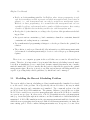
5.1
Modelling the Harvest Scheduling Problem
The way in which a harvest scheduling problem is mathematically formulated is referred
to as the model of the problem. More specifically, the model refers to the way in which
the objective function and constraints are formulated. Two commonly spoken of models
are Model I and Model II formulations. The primary difference between the two is that
Model I choice variables are acres in a management unit, whereas Model II choice variables
are acres in an age class. In other words, a Model I formulation tracks each management
unit (e.g. forest stand) throughout its existence, and the identification of individual stands is
maintained. A Model II formulation tracks a given management unit until it is clearcut, after
which the new regenerating stand is merged with all other management units cut during the
same cutting period. These combined management units now, at age zero, become a new
Habplan User Manual
12
management unit (age class), with a new identity. Thus, Model I looks at a management unit
and all the alternatives for managing it throughout a planning horizon (number of years in
the future for which a plan or projection is made), which is often multiple rotations. Model
II looks at an age class and the alternatives for managing that age class for a single rotation.
Habplan uses a Model I formulation. The primary advantage of using a Model I rather
than a Model II formulation is the ability to track all management units throughout their existence, which is a requirement when spatial constraints are included in a harvest scheduling
problem.
5.2
Solving the Harvest Scheduling Problem
As opposed to the model itself, the solution technique is the mathematical programming
technique that is used to solve the model. Two discrete catagories of solution algorithms are
1) optimization and 2) simulation.
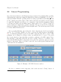
Linear programming is a widely used mathematical programming tool for computing
optimal solutions to problems involving the allocation of scarce resources. This optimization
algorithm seeks to improve on simulation outputs by sorting through harvest schedules to
produce elevated combinations of objectives. This is done through the ranking of possible
harvest schedules using an objective function. LP was the first optimization method applied
to maximize harvestable volumes or Net Present Values (NPV), and has thus been around
for many years. The primary shortcoming of LP, however, is its limited ability to account
for spatial aspects of harvest scheduling. Thus, what LP suggests to be the optimal solution
usually turns out to be impossible in the real world.
With increasing emphasis placed on spatial concerns such as fragmentation and patch
size in forest management, and the continued introduction of new spatially-oriented environmental and social constraints, spatial simulation techniques continue to be developed.
These simulation algorithms mimic processes in harvest scheduling, seeking ultimately to
arrive at the same outcome that would occur had the situation been played out in real life.
Thus, these simulation algorithms do not offer one optimal solution, as does LP, but rather,
in principal, they compute a range of harvest schedules that are all feasible. At this stage,
we are not aware of any available simulation-based harvest-scheduling packages that report
multiple feasible solutions. Other harvest scheduling packages seem to simply converge on
the “best” solution. Habplan, however, does have the capability to report multiple feasible
solutions. Although these simulation techniques may not be capable of finding the perfectly
optimal solution, they are capable of finding near-optimal solutions, sometimes within a few
Habplan User Manual
13
percent of the optimal.
Habplan uses a statistical simulation approach based on the Metropolis algorithm. It
does, however, also have a LP capability, which is useful in that it allows the user to compare
the Metropolis algorithm solution to the non-spatial optimal solution.
6
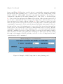
Main Habplan Menu
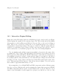
When you execute Habplan, a window opens with a textfield to fill out:
N of Iterations - How many iterations should the program try before it stops The Edit
menu is used to open or close objective function component forms. The Graph menu allows
you to open graphs for components that have associated graphs, but graphs are available
only when a component is added to the objective function.
The checkboxes allow you to add components to the objective function. The unit checkbox allows you to enforce management units.
There are also pull down menus. The File menu has choices to: Open or Save settings
from the component forms to a file. Output lets you periodically save results about the
current schedule and each Flow and Block component to a file.
The Edit menu is used to open or close objective function component forms and the
Management Unit form. The Graph menu allows you to open graphs for components that
have associated graphs, but graphs are available only when a component is added to the
objective function.
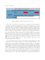
The Tool menu allows you to open the remote control window to run Habplan simultaneously on multiple computers. Remote control will probably be discontinued in the future.
Most networks now have firewalls that prevent this from working. It also lets you open a
fitness function window to specify how the best schedule is determined.
The Miscellaneous menu (Misc) controls things like the license and sound. It also has an
option to reconfigure Habplan to show different objective function components, which is a
very important feature.
The Help menu (Help) provides some immediate help text. However, the on-line or pdf
Habplan User Manual
14
version of the manual is likely to be the most up to date reference.
6.1
Management Units
Habplan allows you to place individual polygons into management units. These might also
be called blocks or cutting units. This addresses two issues: how to handle (1) multi-stand
cutting units and (2) multi-part stands. They both result from the forester’s desire to group
individual polygons and apply the same management regime to the group. Habplan allows
you to input a text file with 2 columns. Just click on the checkBox on the main Habplan
window to read the file that you specify in the unitForm.
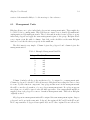
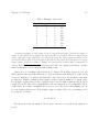
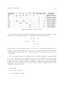
The file format is very simple. Column 1 gives the polygon id and column 2 gives the
management unit id.
Table 1: Example Management Unit File
Polygon ID
1
2
3
4
5
6
7
8
Unit ID
cu1
cu1
cu1
cu1
cu2
cu2
cu3
cu3
Column 1 includes all the polygons that need to be assigned to a management unit.
Column 1 polygon id’s should be already known to Habplan from reading flow data or data
for some objective function component. Any polygons that aren’t in the management unit
file will become the sole member of a one polygon management unit. If a polygon appears
more than once, it will be ignored after the first appearance. If no management unit file is
supplied, then each polygon becomes a 1 member management unit. This is how Habplan
originally worked.
All polygons in a management unit will be assigned the same management regime. Supose
polygons 1 and 2 are in the same unit. Polygon 1 has regimes A,B,C and D in the Flow and
Bio2 component files. Polygon 2 has regimes A,B, and C. Since regime D is not allowed for
Habplan User Manual
15
Polygon 2, then it won’t be allowed for polygon 1, because its in the same management unit
with polygon 2. You need to keep this in mind when assigning polygons to units.
You might also want to break multi-part stands into individual polygons and then assign
those polygons to the same unit. Multi-part stands become a problem when one wants to
control block sizes and other spatial patterns. For example, consider a 2 polygon stand, where
each polygon is 100 acres. Polygon A has 2 neighbors and polygon B has 3 neighbors, but
they don’t share any neighbors. If this is treated as a single stand, then it is a 200 acre stand
with 5 neighbors. This becomes unnecessarily restrictive when trying to control blocksize.
When the stand is split into its component polygons, this problem goes away. Putting the
component polygons into the same unit forces them to get the same management regime.
7
Flow Component
The Flow components are the most important and flexible component currently available
in Habplan. They provide basic control of the flow of outputs. An objective function with
one flow component and multiple CCFlow components might be more useful than having
multiple Flows. However, if you want to simultaneously control multiple flows, use the config
option to make the flows available. This kind of objective function in Habplan notation looks
like:
OBJ = F1 + F2 + F3 ...
Component F1 would require a file giving the full information for the flow involved, as
would components F2 and F3. The implication here is that a management option applied to
a polygon yields multiple outputs of different kinds and possibly at different dates. The usual
output considered in harvest scheduling is wood by weight, volume, or present net value.
Presumably, you might want a flow term for each of these. However, if there is only 1 year of
output for each regime, this situation could be more efficiently handled with CCFlow terms
if the outputs occur in the same year. This way, you don’t carry the memory overhead of
reading in the larger Flow files for each component. (Habplan holds everything in memory).
Another use for multiple Flows might be where there are intermediate operations, like
thinning, that occur at different years from the principal flows. In this case, you might want
an extra flow term to control thinning outputs, or habitat creation efforts. Such outputs
might be specified in terms of wood, costs, area, or sediments.
Habplan User Manual
16
Multiple flows are also used for multi-district scheduling. Suppose F1 and F2 are the
flows for district1 and district2. Then F1 and F2 read their data from a file. F3 would
represent the regional level flow and doesn’t require it’s own file, instead you type F1; F2 in
place of the file name on the F3 entry form to indicate that F3 ”owns” F1 and F2. Note that
there is no limit to the hierarchy that can be created, e.g. districts can have sub-districts,
which can have sub-sub-districts. Only the lowest level flows in the hierarchy will actually
read data, since higher levels get their data from the sub-flows that they own. Likewise,
the lowest level flows can each have their own block and CCFlow components, but higher
level flows (like F1) can’t. The rule of thumb here is that any flow that directly reads
data can have associated Block and CCFlow components. A flow component that gets its
data from sub-Flow components can’t have a Block or CCFlow component. A block file for
multi-district scheduling can only contain the polygons that belong in the sub-district.
Bio-2 and Spatial model components can be used within the context of multi-district
scheduling. However, Bio-2 and SMOD components must read data that contains all of the
polygons from each sub-district. Bio-2 and SMOD must be viewed as global components
that apply to all districts. Contact NCASI if you would like an example data set to evaluate
multi-district scheduling capabilities.
7.1
Linked Flows
This is a new feature that was first made available in version 3. You’ll notice a pull down
menu on each flow edit form called “Link” (unless there is only 1 flow component). Click
on the “Link” menu and you’ll see a checkbox for each of the other Flows in the objective
function. You can link other flow components to this flow component by checking the box.
Specifically, this links all of the goal sliders and the goal +/- textfield.
Suppose you check the F2 box uder the “Link” menu for F1. This means that any
adjustments you make to sliders on F1 will occur simultaneously on F2. You can link as
many Flows as you like. This may be useful for runs that have lots of Flow components
where some of them are related. You can not link F2 to F1 and also link F1 to F2. This is
a circularity that would create problems.
Note that when you link F2 from F1, then slider changes on F1 effect F2. However, slider
changes on F2 will not effect F1.
Habplan User Manual
7.2
17
Flow Data
Each flow component requires a data set. For each polygon, there is one row for each regime
that is allowed. A disallowed regime is simply not included in the data for the polygon, which
prevents that regime from ever being assigned to that polygon. For example, maybe you
can’t allow clearcutting for polygon 10 because it’s near a stream. Be careful with multiple
flows that each flow dataset contains all allowed regimes, even if some of the regimes produce
0 output for some of the flows.
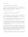
A simple example of some flow data follows. Note that outputs are polygon totals, NOT
per-acre or per-hectare. For regimes with multiple output years, the format calls for entering
the years and then the outputs, so if polygon 2 had 2 years of output for option 3, you have:
2 3 yr1 yr2 out1 out2 . For the data depicted below, polygon 1 can only be assigned option
16, while polygon 2 could have options 1-8.
Habplan User Manual
18
Table 2: Example of flow data
Poly ID Regime ID
1
16
2
1
2
2
2
3
2
4
2
5
2
6
2
7
2
8
Year Output
0
0
1
179
2
187
3
196
4
204
5
210
6
216
7
222
8
228
In general, polygon id and regime id can be any arbitrary name. Instead of polygon 1,
regime 1, you could name it polygon P1 and regime R1, for example. However, using integer
regime values has some advantage, since the entry forms for some components allow you to
use notation like 1-15 to indicate regimes 1 through 15. Of course, this only works for integer
regime names. Don’t use regime 0. Regime 0 is used by the biological type 1 component to
indicate that data being input are not training data. Also, the output is an integer – it takes
much less memory to store integers than floating points.
Option 16 is a do-nothing option in the above dataset. Do nothing options are denoted
with output=0 and optionally with year=0 . Year=0 indicates that this period of this option
does not contribute to blocksizes, and this will be auto-detected by the blocksize component
for this flow. Finally, remember that regimes can have variable numbers of output years.
For example, regime 1 may produce output in years 1 and 21, while regime 20 only produces
output in year 20. There is no requirement for the data input file to be rectangular for flow
components. If you like rectangular files, however, you could create extra dummy periods
for your regimes with year=0. For example, suppose regime 2 has a second dummy period
for polygon 1 as follows:
1 2 1 0 120 0
The first period has an output of 120 for year 1 and the second period has output 0 in
year 0.
Habplan User Manual
7.2.1
19
Flow Data for PreCut Stands: Spatial Issues
The beginning of a planning horizon is usually designated as year 1 in Habplan. However,
there will often be “pre-cut” stands that were cut 1, 2 or more years before the start of the
planning horizon. These stands will contribute to blocksizes in the first few years of the
planning horizon (until they green-up) and should be accounted for.
Habplan provides two ways to do this:
1. Start the planning horizon several years ahead of the current year.
2. Designate pre-cut years in a flow file as negative numbers.
The first method requires you to designate the early years of the planning horizon as
“byGone” on the Habplan Flow Edit Form. The regimes that were actually applied are
supplied for the stands in the byGone years. Habplan makes no effort to schedule things in
these byGone years (2), since they are in fact already scheduled.
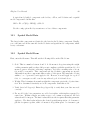
The second approach may often be easier to implement and Habread can help you. The
idea is to create a Flow dataset that has years when precutting occurred designated by -1=”1
year before the start of the planning horizon”, -2=”2 years before”, etc.
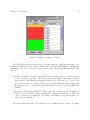
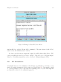
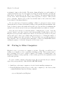
This is what (Figure 1) the Flow data might look like when precutting is implemented.
Notice that precut stands have a negative year value in the first Year column and the
corresponding output is 0. In fact, the output for a precut management action is irrelevant,
since Habplan will only display results for years that are greater than or equal to the first
year of the planning horizon.
You only need to use this feature for Flow components that have a Block subcomponent,
otherwise its a waste of time. The block component will recognize the negative years and
will incorporate the precut stands into blocks where appropriate. For example, suppose the
planning horizon starts in year 1, and the green-up window is 3 years. Then a stand that
was precut in year 0 will have a -1 year designation in the first year column of the flow data.
This same stand will contribute to blocksizes for any neighbors that are cut in years 1, 2 or
3. Likewise, a stand that was cut 3 years before year 1 is designated with -3 in the Year
column, and would only effect blocksizes of neighbors cut in year 1.
A final thing to consider is the effect of precutting on the number of actions that occur
for a regime. Precutting simply adds an extra action time to the regime. For example, if
Habplan User Manual
20
the regime would normally have one action time that represents clearcutting, it would have
2 actions when precutting is designated.
7.3
Flow Form
You fill out a flowform to control the behavior of a flow component. After entering the file
name, you have:
1. Checking the no model check box will allow you to enter specific flow (year,target)
value pairs separated by ’;’ for each year. Otherwise you use internally generated
target values that are based on an initial starting value and interest rate for trend.
Figure 1: Example of Flow Data for Precut Stands
Habplan User Manual
21
You can also enter a few (year,target) values to pin things down, and Habplan will
internally generate the remaining target values as follows. The gap between two years
is filled via linear interpolation. After the last year, a free floating spline is used that
is influenced by the slope value. So, if you have 50 years and specify 1,100000 and
40,150000, this is what happens. A straight line is drawn from year 1 to year 40 that
goes from 100000 to 150000 for target values. After year 40, the target is allowed to
float somewhat according to your slope and goal settings.
2. ByGone Yrs - These are years that have already past, i.e. these regimes have already
been applied and polygons managed under these regimes have no other management
option. This lets the program know that it need not worry about attaining goals for
these years since it is a byGone era. It is useful to include as many byGone years
as green-up requires in order to have correct blocksizes for the first few years. Note
that goals for year 0 in the flow component don’t apply when year 1 is byGone. Make
sure that you enter each byGone year. Suppose there are 6 such years and they are
1-6. Note that you are allowed to use the shortcut 1-6. Alternatively, you could have
written 1;2-4,5 6. Note that ’,’ ’;’ and blank are allowed separators.
Habplan doesn’t worry about trying to follow the target for byGone years, since it
assumes it must assign the single regime that you include in the input data file for
polygons managed in these years. A useful concept: if you don’t want Habplan to
worry about certain years being on target, you could declare them as byGone even if
they really aren’t!! However, this would mean that blocksizes for these years would be
allowed to go out of bounds also.
There is another way to handle precut stands described elsewhere 7.2.1.
3. Time 0 starting flow: This is the level at which you want the flow to start. If year 1 is
denoted as byGone on the main menu, then Time 0 entries are unnecessary and don’t
appear.
4. Time 0 goal: The is 1 minus the amount you will allow the starting value to deviate
from your specification in (1). Actually, it is allowed to vary within + or - 5 percent of
what you specify. If you enter a number that is not between 0 and 1, the textfield will
turn red to warn you. A 1 means you want to be within 95% of the specified starting
value. A .5 means within about 50% is close enough.
5. Threshold: You can enter a - value and a + value. The minus is subtracted from
the target and the plus is added to the target to produce lower and upper thresholds.
As long as yearly flows fall within these thresholds, Habplan assumes they are OK.
Values that fall outside the thresholds will be constrained according to your Flow
Goal explained below. The default thresholds + and - values are 0, which means that
Habplan tries to keep flows close to the target values.
Habplan User Manual
22
6. Flow goal: This has the same purpose as the time 0 goal, except it also applies to
deviations from 1 year to the next. The actual deviations are displayed in a black strip
at the bottom of the form as the algorithm iterates. These may vary considerably from
your request, at the beginning of the run. Habplan will adjust the Flow and Time 0
weights in an effort to bring the flows within yur specification.
7. Goal +/-: This allows you to specify the +/- limits on the Flow goal. For example,
if you specify Flow goal=.9 and Goal +/-=.05, then deviations from the target of .85
to .95 are allowed. Most other objective function components have +/- .05 hard-wired
in an effort to minimize required input from the user. Note that if you set Flow goal
= .9 and Goal +/-=0, then only .9 is acceptable to Habplan, i.e .91 is too much and
.89 is not enough, so the weights will almost always be changing. You might want to
use thresholds and then specify a strict goal of 1.0 to keep flows strictly within the
thresholds.
8. Interest rate (slope) for flow model: Must be a number between -1 and 1. This determines the trend over time in your flow. For example, .03 means try for a 3 percent
compounded annually rate of increase.
9. Flow Model Weight: This is the weight that the flow component gets in the objective
function. There is no way to know what this should be in advance, so the program
figures it out iteratively. It is best to set all weights to 1.0 at the beginning of a run.
10. Time 0 weight: The same as the Flow adaptive parameter, but applies to keeping the
starting value under control. It’s usually best to start all adaptive parameters at 1.0
at the beginning of a run and let the computer determine their values. However, as
you gain experience, you can give a component a head start by setting the initial value
of adaptive parameters.
11. Verify data for Polygon#: Enter the polygon id# to verify that your data was read
correctly.
7.4
Flow Summary
The flow component is the most versatile component and therefore the most important and
complicated to use. The flow component allows you to specify target values via an internal
smoothing function or directly as specific annual values. The smoothing function is controlled
by specifying a slope rate between -1 and 1. If there are no byGone years at the beginning
of the period, you must specify a time 0 starting value. The goals determine how close to
the starting value and targets that you want to be. You can also specify thresholds as +
Habplan User Manual
23
and - deviations from the targets. The implication is that you are indifferent to all flow
values within the thresholds. When flows fall outside the thresholds, then your goals will be
applied. A goal of 1.0 implies you want everything inside the thresholds, whereas a goal of
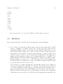
.8 means you’ll allow some values outside the thresholds. This graph shows a flow that is
flexible within the upper and lower thresholds, but is fairly tightly constrained to be within
the thresholds. The first 4 years are byGone, so they are ignored for flow purposes. An
example of such a flow graph can be seen in Figure 2.
Figure 2: Example of a flow graph
You can also have a mix of specified and smoothed targets. For example, if you want the
flow for year 10 to be 100000, just specify 10,100000; in the flowform textarea. (Check the
noModel box to get to this textarea.) This will set the year 10 target to 100000, but use the
smoothing model for the other years. By specifically putting values for each year, you can
create any desired flow. However, try the internal smoothing model first before bothering to
enter specific targets.
The flow component also allows for multi-district scheduling. The idea here is that flows
can have subFlows and subFlows can have sub-subFlows etc. Suppose that F3 has F1 and
F2 as subflows. Indicate this in the file/subFlows textfield as follows: F1;F2; on FlowForm
3. The F1 and F2 file/subFlow field should have file names, because they would read data,
and F3 would use their data to create a superFlow. This allows you to control the subFlows,
Habplan User Manual
24
F1 and F2, to look at their effect on the superFlow, F3. Conversely, you can control F3
and look at what happens to F1 and F2. This feature should be useful whenever you have
subregions that need to be tracked separately.
You might be able to use a flow component to control the amount of inventory at the end
of the planning period, if you are clever. For example, you could create a flow component
where the input data gives the age of the stand at the end of the planning period that would
result from each management regime. The output associated with this age could be the acres
in the stand. Then the resulting flow graph will give the acres by age-class at the end of the
period.
8
CCFlow Component
This component depends on a parent flow component for much of its data. Typically,
this component would be used to control clearcut flow. You can have as many of these
components as you need. Here’s a possible use for multiple CCFlow components. Suppose
you are scheduling for several districts. You could specify 1 main flow component to control
the overall flow from the combined districts, then you could have a CCFlow component for
each district. This would allow you to keep within-district cut levels relatively even over
time. Suppose there are 2 districts. This model would be written in Habplan notation as:
OBJ = F1 + C1(1) + F2+ C2(1) + F3
You’d have to use the config option to get the extra CCFlow components. In order for
this model to work, you’d give each CCFLow component the acreage of the stands within
it’s respective district. Note that super-Flow components, i.e. flows that have sub-flows,
can’t have CCFlow or Block components.
The ccFlow graphs show (1) ccFlow versus the target, and (2) the Flow/ccFlow ratio.
This might typically be the volume per acre ratio if Flow is volume and ccFlow is controlling
acres cut.
8.1
CCFlow Data
The CCFlow data format is very simple. There is 1 row for each polygon, unless you want the
polygon’s CCFlow value to default to 0. There are just 2 columns containing: the polygon
Habplan User Manual
25
id, and the CCFlow value. Usually the value is polygon size. Note that this could have some
limitations when your regimes have multi-year outputs. The single CCFlow value must apply
over the multiple years. The assumption is that polygon size remains constant, and there
might be other variables that are constant as well. However, for schedules involving only
single year regimes, this limitation doesn’t apply. To make it clear, here’s what CCFlow
data might look like for polygons 1-3:
1 100
2 23
3 56
This component can use the same file that the BlockSize component uses. It will ignore
the extra information required by the blocksize component. The CCFlow component is
convenient when it meets your needs. However, for multi-year regimes, you may need to
create another Flow component to get the job done.
8.2
CCFlow Form
First, enter the file name. Then fill out the following fields on the ccFlow form:
1. Now you have to specify the CC options, which are usually the ones that denote
clearcutting. Suppose there are 15 such options and they are options 1-15. Note
that you are allowed to use the shortcut 1-15. Alternatively, you could have written
1,2,3,4-12,13;14 15. Note that ’,’ ’;’ and blank are allowed separators. When options
don’t use integer names, you might need to name each CC option specifically. When
regimes (options) are multi-period you must specify regime@period pairs. So if regimes
1 through 4 for period 2 contribute to CCFlow you’d write:
1@2; 2@2; 3@2; 4@2;
You can also indicate a regime prefix,which is automatically expanded. For example,
if your clearcut regimes all begin with “CC”, then put “)CC” into the CCFLOW form
text field. Don’t include “, but the “)” indicates that this is a prefix. Suppose you
have regimes that begin with “CT” to mean clearcut as the first action and thinning
as the second action. Indicate this to Habplan as )CT@1, which says to include the
first period of all regimes that begin with CT.
Any combinations of this entry notation are allowed, so )CC;PT@1; gets all regimes
that begin with CC, and the first period of regime PT.
Habplan User Manual
26
Note that this system only works when your regime names have an intrinsic meaning
that applies across all stands. Clicking on the window will cause the CC regimes that
Habplan is using to be listed for you. You may need to hold the mouse button down
while entering the CC regimes to prevent listing from occurring.
2. Goal: This is 1 minus the deviation around the trend line as well as the year to year
deviation. When the program is running, you see the current actual values in the black
display area on the form. The entered number must be between 0 and 1 or you see
red. This does the same thing as the Flow Goal mentioned above.
3. Interest rate for ccFlow model: A number between -1 and 1 that determines the slope
of the trend line.
4. Weight: This determines how much weight this component gets in the objective function. It is determined iteratively as for all components. Set to 1.0 at the beginning.
5. Verify data for Polygon #: Enter the polygon id# to verify that your data was read
correctly.
9
Blocksize Component
This component controls minimum and maximum blocksize. However, it also provides information on average blocksize, which can be indirectly controlled. Blocksize is a subcomponent
of flow, since it needs to know when the flows occur to compute blocksizes. A block is defined by a target polygon and all of its neighbors that were subjected to a ”block” treatment
within a specified time window. Typically the block treatment is clearcutting and the time
window allows for ’green-up’ to occur. This component can also be used to enforce cutting
limits within any block of stands by making each stand in the block a neighbor of every other
stand in the block. For this special use, only first order neighbors need to be considered in
the block size computations. By definition, block sizes must be re-evaluated annually. At
any given block, some stands will grow out of the block and new ones may enter each year.
A parent Flow component, say F1, can have any number of dependent block components,
BK1(1), ... , BKn(1). You might want to control maximum cluster size of more than one
kind of treatment. Maybe you don’t want too much old-growth forest in one location, or
too much thinning. You might also want to have different blocksizes for different green-up
periods. If you never want to cut more than 100 acres or less than 20 in a given year, for
example, have a BK component with a 0 year green-up to specify this. Computing blocksizes is computationally demanding, so expect the program to run slower when a blocksize
Habplan User Manual
27
component is in the model. A typical objective function with 1 component each for flow,
ccFlow, and blocksize looks like this:
OBJ = F1 + C1(1) + BK1(1)
Use the config option if you want more components.
9.1
Block Data
The data for the blocksize component must include information about each stand’s size and
a list of its neighbors. All input files to Habplan are ascii, so you must produce the neighbor
list by some external means, e.g. a GIS package, and output it to an ascii file. In theory, the
size variable could be replaced with something else that is constant for the stand over time
for regimes that have multi-year outputs. For single year regimes, the variable replacing
size could be almost anything. For example, use sediment yield associated with a regime
and the blocksize component will prevent you from producing too much sediment within a
block of stands. Whereas the flow component controls production over time, the blocksize
component can control production spatially.
Let’s look at some data. The first 2 columns are polygon id#, and size. The data can
have one or more neighbors on each line and use one or more lines per polygon. You can
pad the file with 0’s to make it rectangular if you like, and Habplan knows to ignore them
(notice the entry for polygon #8). The data below show that polygon 1 has size=124 and 2
neighbors, which are polygons 2 and 4. This is the 1 row per polygon format. Fortunately,
the data show that polygon 2 and 4 also consider polygon 1 to be a neighbor. Habplan
doesn’t look for logical consistency within this file, that’s your job.
1
2
3
4
5
6
7
8
124 2 4
313
31 2
65 1
145 6
74 5 7
43 6
33 9 414 0 0 0 0
Here is the same input data in a one neighbor per line format.
Habplan User Manual
1
1
2
2
3
4
5
6
6
7
8
8
28
124 2
124 4
31
33
31 2
65 1
145 6
74 5
74 7
43 6
33 9
33 414
This same data file can be used by the CCFlow and SpaceMod components.
9.2
BlockForm
First, enter the file name. Then fill out the following fields on the BlockForm
1. Now you have to specify the notBlock regimes, which are the regimes that are NOT
going to contribute to blocksizes. This is the opposite approach to that used for
entering the CCFlow regimes. (At the time, it seemed like the right thing to do.) As
with entering CCFlow regimes, use a dash to indicate inclusion of many regimes (1-3
is the same as 1,2,3). Separate options in your list with space, comma or semicolon. A
valid list would be 1-3,4,5;6;7 8 or you’d get the same result with 1-8. For multi-period
regimes, specify regime@period pairs, e.g. 3@2 means that period 2 of regime 3 does
NOT contribute to block size. When a single number is entered for a notBlock regime,
Habplan assumes it is for period 1, i.e. 10 is the same as 10@1. When regimes don’t
use integer names, you might have to name each notBlock regime specifically, unless
you can use prefix notation described below.
You can indicate a regime prefix,which is automatically expanded. For example, if
your notblock regimes all begin with “T”, then put “)T” into the Block form. The
“)” indicates that this is a prefix. Suppose you have regimes that begin with “CT” to
mean clearcut as the first action and thinning as the second action. Indicate this to
Habplan as )CT@2, which says period 2 of CT regimes is notBlock. Any combinations
of this entry notation are allowed, so )T;PC@1; gets all regimes that begin with T, and
Habplan User Manual
29
the first period of regime PC. Finally, )CTT@2@3 would get periods 2 and 3 of CTT
regimes, and )CTCT@2@4 would get periods 2 and 4 of CTCT regimes.
Note that this system only works when your regime names have an intrinsic meaning
that applies across all stands. Clicking on the window will cause the notBlock regimes
that Habplan is using to be listed for you. You may need to hold the mouse button
down while entering the notBlock regimes to prevent listing from occurring.
A regime with output year=0 is a convenient way to specify a do-nothing option in the
parent FLOW data. Habplan will automatically detect year 0 options and treat them
as notBlock options. Click on the notBlock textArea after reading the data to see what
notBlock options were auto-detected. This will also give a list of any notBlock options
not found in the parent Flow Data. Make sure these are not typos. Sometimes you
may have a valid notBlock option that was never allowed for any of the polygons. In
this case it is OK to include it as a notBlock, even though it will not occur with the
current dataset. It may, however, occur in a future dataset.
Finally, you can put notBlock options in a dataset, rather than manually enter them
on the form. This might be useful if there are a lot of notBlock options that can’t
be neatly specified with a prefix. Suppose you create a text file called notBlocks.dat.
Put regime@period pairs separated by spaces, commas or semicolons in the file. There
can be 1 or more regime@period pairs per line. If you put the file in a sub-directory
of the Habplan3/example directory called myProject, then enter the following in the
notBlock entry field: ”myProject/notBlocks.dat” without the quotes. Then Habplan
will read the notBlock options from this file. If you put the file elsewhere, you’ll need
to enter a complete path, which also reduces the portability of this project.
2. Kill SmallBlocks: This button should be pushed as a last resort. There may be s1
thru 15 being kept together with some cases where the standard Metropolis algorithm
won’t build all blocks up to the minimum size specified. If you push this button, then
at the beginning of the next iteration, Habplan will set polygons in small blocks to
a doNothing option if the doNothing option is valid (see preparing input data). This
will eliminate the small blocks, at least temporarily. Make sure you give the algorithm
enough time to attempt to work its stochastic magic before you push this button. Note
that the button becomes disabled until the small blocks killSmallBlocks has completed
execution. Blocks smaller than the current Target Min are impacted by this button.
3. Green Up: This determines how many years it takes after a block treatment for the
polygon to grow out of the block. So, if Green up=2, a stand clearcut in 2000 is considered to be ”greened-up” beginning in 2003. Green up=0 implies that it is greened-up
the year after cutting.
4. Min and Max Blocksize: This is the min and max block sizes that you will allow. When
Habplan User Manual
30
Habplan is running you will see the current Min and Max (over all years) displayed at
the bottom of the BlockSize edit form. The Target Min value being displayed is the
current minimum that Habplan is trying for. This target minimum is incrementally
increased until Habplan attains your specified Min, or until it can’t go any further.
Sometimes you may need to reduce the goals on other components in the objective
function to attain the desired minimum. When the goal is less than 1.0, the incremental
approach is not used.
5. 1st Order Neighbors: Check this if you want block sizes determined only on the basis
of 1st order neighbors. Normally you DO NOT want this. This option (with green
up window=0) is useful when you want to use a blocksize component to ensure that
a minimum amount of cutting will occur each year in specified districts or cutting
blocks. In that case, each polygon in a cutting block should have all other polygons in
the block declared as neighbors. This means that once Habplan has looked at the 1st
order neighbors, it has all possible neighbors and is wasting time to look for second
order neighbors. The ”Allow 0 Flow option” on the flowform could get the same result,
but might not be as effective. When appropriate, the 1st order option can greatly speed
up processing.
6. Goal: This is how tolerant you are to allowing some blocks to being outside the size
limits. A value of 1.0 means all blocks must comply. Any value for Tolerance greater
than 0 and less than 1 is treated like the deviations for flow and ccFlow, i.e. it means
that a proportion of the blocks, within +or- 5 percent of the entered tolerance, should
be less than the maximum. Specify a value of 1.0 to make the maximum blocksize
totally constraining. Note that this isn’t linear programming (LP). Therefore, if you
enter a maximum blocksize of 150 and many of your stands are of size 200, the program
will still run and find solutions that violate your constraint. However, all of the larger
stands should eventually be assigned to NotBlock options. Even if you only allow
assignment of the 200 acre stands to block options (by indicating this in the flow data)
Habplan will give you solutions that violate the blocksize restriction, whereas LP would
declare the problem to be infeasible. Note that the BK component check box may turn
red and indicate convergence even though there are still blocksize violations. This is
because Habplan is not finding any better alternative management regimes to clear up
the violations.
7. Weight: This determines how much weight this component gets in the objective function. It is determined iteratively as for all components. To control blocksize, this
parameter may eventually become very large, say 1.0E38. Regardless, its a good idea
to let it start at 1.0 and slowly increase. Otherwise, the blocksize constraint will become limiting too early in t1 thru 15 being kept together with he process and may
result in a poor solution. It may take several hundred iterations before blocksize is
Habplan User Manual
31
under control, so be patient, this is a simulation process that can’t be rushed. If it’s
taking too long, maybe this will help you convince your boss to bedecisive and buy
you a new computer.
8. Verify data for Polygon #: Enter the polygon id# to verify that your data was read
correctly.
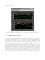
9.3
Block Graphs
There are 2 graphs that accompany each block objective function component. Both graphs
have an X-axis that goes from 1 through the number of years in the planning horizon. The
graphs display the following information:
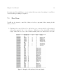
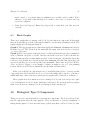
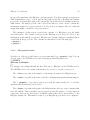
Graph 1) The upper graph shows 3 lines that display the Minimum, Maximum and Average
Blocksize by year. The Y-axis is in the units that the input data used for size of polygon,
e.g. acres or hectares.
Graph 2) The lower graph of the pair shows 3 additional lines that give the accumulated
areas of different categories of blocks. One line shows the total area of all blocks that are
within the min and max blocksize limits specified on the block form. Another line shows the
total area of blocks that are below the specified size minimum. The third line shows the total
area in blocks that are above the specified size maximum. These lines are labeled Within,
Above and Below . Figure 3 is an example of what you might see for a 15 year planning
horizon, when not all blocks are within the specified min and max values.
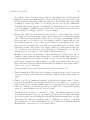
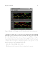
If the goal on the Block component is set to 1.0 and Habplan is able to converge for this
component, then all blocks that are above or below the limits will be made to conform to
within limit sizes. After some more iterations, the graphs will look like those in Figure 4.
These graphs show how much area is in a managed block each year and provide quite
a lot of information about block size distribution and trend. For green-up windows greater
than 0, not all area in a managed block was managed in the current year.
10
Biological Type I Component
This is a top level component with no dependent subcomponents. The biological type I and
type II components serve the same purpose. They are intended to bias the assignment of
management regimes to better meet the users goals in ways that could not be met by other
Habplan User Manual
32
Figure 3: Example of a block graph - not all blocks within specified min and max values
components. For example, suppose you know the present net value (PNV) that results from
each regime for each polygon. The biological components can be used to put pressure on
the scheduler (Habplan) to assign the regimes that produce the most PNV to each polygon.
You can have as many of these components as you want in the model. Maybe you want to
use one biological component to bias the result toward more PNV and another to bias the
result toward less sediment yield or more habitat for owls. Of course, you have to know how
to model the effect of each regime on owl habitat to implement the owl component. A model
with 2 biological type I components would look like this:
OBJ = F1 + C1(1) + BK1(1) + BioI1 + BioI2
Edit the properties file if you want a different configuration of components.
Habplan User Manual
33
Figure 4: Example of a block graph - all blocks within specified min and max values
10.1
Biological Type I Data
The Type I biological component uses maximum likelihood classification to determine the
desirability of each management regime for each stand. The user must supply training data
that indicates for each regime a set of polygons that represent the best situations for that
particular regime. Here’s an unsophisticated example for how this component could be used
to create wildlife habitat. First you need to decide what the relevant variables are – lets
suppose they are a) maximum tree diameter at time 0, b) slope, c) distance to water. Now
you must pick groups of stands that represent the ideal for each regime. Suppose the clearcut
regimes would be represented by a set of stands: with small to medium sized trees, with little
slope, and that are far from water. Conversely, the do-nothing regimes could be represented
by stands: with big trees, having steep slopes, and that are near to water. Selection cut
regimes would be represented by stands between these extremes. Now you have created a
BioI component that will bias the management schedule toward making desirable habitat.
Habplan User Manual
34
Use a Flow component to keep the amount of this habitat even over time.
What data are required? The first column is polygon id#. Column 2 indicates whether
this polygon is a trainer – a 0 means no, anything else indicates the regime that the polygon
is a trainer for. The remaining columns are the values of the biological variables the user
selected. These variables should be continuous and apply to the polygon throughout the
regime. For regimes with only 1 output year, this is no problem – for multiple output years
it becomes more limiting. For example, slope applies throughout a regime, but number of
loblolly pines at time 0 may not be relevant for a multiyear output regime, since the polygon
might get clearcut and replanted midway through the regime.
The data below indicate that polygons 1 and 2 are not trainers. Polygon 3-6 are trainers
for options 16, 15, 5, and 10 respectively. Obviously, a polygon can only serve as a trainer
for 1 regime. Each option should have at least 10 to 20 trainer polygons so that accurate
training statistics are obtained.
1 0 10 124
2 0 263 3
3 16 3456 31
4 15 4451 65
5 5 13534 145
6 10 6782 74
7 0 10 43
8 16 3505 33
9 16 3146 54
10 2 12617 118
11 8 6758 63
The Bio-I component doesn’t influence the determination of valid regimes for apolygon.
Therefore, you can include training data for any subset of the available regimes; i.e. there is
no requirement that every regime have training data included in the Bio-I dataset. When a
regime isn’t present in the Bio-I data, habplan will skip the Bio-I component when considering the assignment of that regime to a polygon.
10.2
Biological Type I Form
First, enter the file name. Then fill out the following fields on the BioI Form:
Habplan User Manual
35
1. N of Biological vars: As you might expect, this is the number of biological variables,
which would be 2 for the example data above.
2. Goal Kind: Selecting max means the goal is relative to the the most that could be
attained if all polygons were assigned to their highest ranking valid regime. This
is not very intuitive, since it’s based on the maximum likelihood assessment of the
regime ranking. So the max value would be the sum of a number associated with the
highest ranking regime for each polygon. That mysterious number is the normal PDF
value that the maximum likelihood ranking is based on. If you set the Goal to 0.8,
then Habplan will try to find schedules that attain 80 percent of this max possible
likelihood summation. Actually, it will consider anywhere from 75% to 85% to be OK.
Remember that the maximum likelihood procedure does the ranking internally for this
component, unlike for Bio-2 where you specify the rankings.
For this component, doing things relative to a maximum may be hard to interpret. If
you prefer, Habplan allows you to control the proportion of polygons that are assigned
to regimes that are at least as good as the Goal Kind value. A value of 1 means you
want the proportion of polygons specified by the Goal (discussed next) to be assigned
to regimes equal in rank to the highest ranking regime. Note that several different
regimes could have the same rank, so you’d be indifferent among them. A value of 2
means you’re indifferent to assignments equal to the 2nd ranking regime and higher.
In the extreme, if there are a total of 10 regimes and the Goal Rank is 10, then you
are indifferent to everything and this Bio-1 component serves no purpose. Note that
the ranking is based on the currently valid regimes for the polygon. Valid regimes can
changedepending on what components are currently in the objective function.
3. Goal: This is the proportion of polygons that should be assigned to regimes that are
at least equal in rank to the Goal Kind value (discussed above). If the proportion is
within + or - 5 percent of your request, then Habplan declares that it has converged
on your goal for this component. If Goal Kind = max, then this is specifying that you
want schedules that attain this proportion of the maximum possible.
4. Weight: This determines how much weight this component gets in the objective function. It is determined iteratively as for all components. As usual, it’s a good idea to
let it start at 1.0 and let the program change it adaptively.
5. Verify data for Polygon #: Enter the polygon id# to verify that your data was read
correctly.
Habplan User Manual
11
36
Biological Type II Component
This is a top level component with no dependent subcomponents. The biological type I
and type II components serve the same purpose. They are used to bias the assignment of
management regimes to better meet the users goals in ways that could not be met by other
components. For example, suppose you know the present net value (PNV) that results from
each regime for each polygon. The biological components can be used to put pressure on
the scheduler (Habplan) to assign the regimes that produce the most PNV to each polygon.
You can have as many of these components as you want in the model. Maybe you want to
use one biological component to bias the result toward more PNV and another to bias the
result toward less sediment yield or more habitat for owls. Of course, you have to know how
to model the effect of each regime on owl habitat to implement the owl component. A model
with 2 biological type II components would look like this:
OBJ = F1 + C1(1) + BK1(1) + BioII1 + BioII2
Use the config option if you want a different configuration of components.
11.1
Biological Type II Data
The Type II biological component is more straight-forward than the type I component.
This approach allows the user to specify the relative ranking of each regime for each stand.
Suppose you want to bias the scheduler toward assigning the regime that produces the most
PNV for each stand. Then you need to assign a ranking for each regime. In situations where
the information is available to use the Type 2 biological approach, it is to be preferred over
the type 1 method, since it provides the user with more control.
Let’s look at some data. The first column is polygon id#, the second is the option and
the last column is the rank. There is one row for each stand and regime. The following
data show a situation where stand 1 must be assigned to regime 2 (the only regime given),
but stand 2 could be assigned to regimes 1-3 with regime 3 being preferred. The size of the
numbers is irrelevant, only the ranking is important. Therefore ranks 1,2,3 give the same
result as .1, 16, 37.
121
Habplan User Manual
37
2 1 0.1
2 2 0.4
2 3 0.5
11.2
Biological Type II Form
First, enter the file name. Then fill out the following fields on the Bio-2 Form:
1. Goal Kind: The default is max which means the goal is relative to the maximum that
would be attained if all polygons were assigned to their highest ranking valid regime.
For example, if the BIO-2 ranking variable is Net Present Value (NPV) and you set
the Goal to 0.8, then Habplan will try to find schedules that attain 80 percent of the
max possible NPV. Actually, it will consider anywhere from 75% to 85% to be OK.
The maximum possible NPV is what would be untained if the highest NPV regime
were assigned to each polygon.
For qualitative rankings, doing things relative to a maximum value doesn’t make sense.
In this case, Habplan allows you to control the proportion of polygons that are assigned
to regimes that are at least as good as the Goal Kind rank. A value of 1 means you
want the proportion of polygons specified by the Goal (discussed next) to be assigned
to regimes equal in rank to the highest ranking regime. Note that several different
regimes could have the same rank, so you’d be indifferent among them. A value of 2
means you’re indifferent to assignments equal to the 2nd ranking regime and higher.
In the extreme, if there are a total of 10 regimes and the Goal Kind rank is 10, then
you are indifferent to everything and this Bio-2 component serves no purpose. Note
that the ranking is based on the values in the Bio-2 input data and the currently valid
regimes for the polygon. Valid regimes can change depending on what components are
currently in the objective function.
2. Goal: This is the proportion of polygons that should be assigned to regimes that are
at least equal in rank to the Goal Kind value (discussed above). If the proportion is
within + or - 5 percent of your request, then Habplan declares that it has converged
on your goal for this component. If Goal Kind = max, then this is specifying that you
want schedules that attain the Goal proportion of the maximum possible.
3. Weight: This determines how much weight this component gets in the objective function. It is determined iteratively as for all components. As usual, it’s a good idea to
Habplan User Manual
38
let it start at 1.0 and let the program increase it as needed.
4. Verify data for Polygon #: Enter the polygon id# to verify that your data was read
correctly.
12
Spatial Model Component
This component allows you to control the spatial juxtaposition of management regimes. For
example, it might be useful to keep operations done in the same year in adjacent stands
to minimize road building and travel costs. Obviously, this objective can conflict with the
desire to keep blocksizes small. Likewise, it might be desirable to make an effort to place
non-clearcutting activities near regimes assigned to streams. In general, this component
operates stochastically to bias the spatial arrangement in desirable ways.
This is a top level component and doesn’t require a specific parent component. You
can have as many of these components as you want. A spatial model component (SMod)
is configured by supplying parameter values to a spatial model. For example, if you want
regime 1 to be close to other regime 1’s you enter 1,1,-1 on the SMod entry form. If you
want to put twice as much effort into keeping regime 1 away from regime 2 polygons you
enter 1,2,2. The first two integer values give the index of the regimes, and the third integer
is the relative weight given to the spatial biasing done by the program. A negative number
means to put the regimes together, a positive number means to keep them apart if possible.
On the SMod entry form, you specify a goal which tells the program in general how hard
to work to achieve your indicated spatial model objectives. A goal of 1 means to work very
hard at it, while a goal of 0.5 means only about 50 percent of the polygons need to comply.
NEW: There are 2 new spatial models that can be selected on the Spatial Model Form:
Model 0 or Model 1 . Model 0 is the old standby that takes 3 input values, i.e. 2 regimes
followed by a positive or negative number to indicate if these regimes should be close or
apart. Model 1 takes 4 input values as follows: DN, BP, 0.75, -1; where DN and BP are the
regimes, 0.5, is an area proportion, -1 says to put DN and BP regimes together.
The Area proportion is a new twist. Suppose the area of the DN polygon is A, then
model1 allows you to request that DN polygons have a specified proportion of their area
in surrounding BP polygons. Input like ”DN,BP,0.75,-1” says that Habplan should try to
set things up so that the area of BP polygons near each DN polygon is at least equal to 75
percent of the DN polygon area. This is more specific than model0, which just says to put
DN and BPpolygons together if possible. Figure 5 is an example of what the input form
Habplan User Manual
39
would look like. Note that only 3 values need to be entered for model0, but if 4 values are
present, model0 ignores the third value (the proportion).
Figure 5: Example of spatial model form
You might want more than 1 spatial model component to give different levels of emphasis
to different spatial goals. For example, you might feel strongly about keeping regimes 1 and
2 separated, since 1 is clearcutting and 2 represents an endangered species habitat. At the
same time, you might want regimes 3, 5, and 7 to be close together although this isn’t as
important as keeping 1 and 2 apart.
Habplan User Manual
40
A typical model with 1 component each for flow, ccFlow, and blocksize and a spatial
model component looks like this:
OBJ = F1 + C1(1) + BK1(1) + SMod1
Use the config option file if you want more or less of these components.
12.1
Spatial Model Data
The data for this component are identical to the data for the blocksize component. Usually,
you could just read in the same file for the blocksize and spatial model components, which
is very convenient.
12.2
Spatial Model Form
First, enter the file name. Then fill out the following fields on the SMod form :
1. Goal: This is a number between 0 and 1. A 1.0 means to keep increasing the weight
on this parameter until you have 100 percent compliance with the spatial model. A 0
means to put no effort into achieving compliance. Probably a starting value of about
0.8 would be reasonable. This component and the blocksize components are treated
differently from other components when a value of 1.0 is given. The usual rule of being
within + or - 5 percent doesn’t apply for 1.0. However, it would apply for a goal of
0.99, i.e. convergence would occur for any achieved goal of 0.94 and above.
2. Weight: This determines how much weight this component gets in the objective function. It is determined iteratively as for all components. Start this at 1.0.
3. Verify data for Polygon #: Enter the polygon id# to verify that your data was read
correctly.
4. For model 0, the beta parameters are added as triplets, with triplets separated by
semicolons . Within a triplet, use either a space or a comma as separators. All beta
values should be integers. The first 2 values indicate the 2 regimes that this parameter
applies to. The third value indicates the desired spatial juxtaposition. A -1 means to
put the 2 regimes together, while a 1 means to keep them apart. A -2 means to put
Habplan User Manual
41
twice as much effort as for a -1. The simple example has regimes 1 thru 15 being kept
together with the same effort applied to each regime, i.e. all are set to -1. This would
tend to conflict with the blocksize component, but should lead to more compact and
uniform blocks being cut each year. In this case the regimes indicate which year to
clearcut the stand. Only an entire regime can be specified for this component; there is
no need to indicate the time period.
As mentioned 2 sections above, the Model1 option requires 4 pieces of input instead of
3. The third item is the proportion of area in the second regime that should be surrounding
the first regime. Read the verbage before the Spatial Model Form picture up above for more
on this.
13
Comments on Preparing Input Data
This section includes discussion on naming regimes and the procedure to indicate the valid
regimes for individual polygons. Habplan is very flexible with regard to polygon and regime
names. The next subsection discusses habplan project files. Project files contain settings in
XML format. You can basically use whatever names you have in your current database for
the polygons. Likewise, any regime name can be used, but give serious thought to naming
regimes so that it’s easy to interpret the output. Habplan has to work harder when there
are lots of regimes, so don’t create regimes that represent trivial variations. For example,
cutting in May shouldn’t be considered different from cutting in June. If 2 polygons are
going to be clearcut in 2010 as the only management activity, then they are managed under
the same regime. There should also be a do-nothing regime assigned to each polygon, unless
there is a good reason not to do so, e.g. , the polygon was already cut in a byGone year.
This allows Habplan flexibility in meeting your goals. For example, it may be impossible to
meet blocksize limits unless some polygons are assigned to the do-nothing option (more on
do-nothings in a few paragraphs)
Remember that CCFlow and Block components have a parent Flow component. They
cannot be included in the objective function unless their parent is in too. Their datasets
must include the same polygons that the parent Flow component has in its data. This also
means that any neighbors in the Block data must show up in the parent Flow data. Usually,
you will use the Block data for the CCFlow component as well. There is some error checking
when the data are read that should warn you about these problems, which cannot be ignored
or Habplan will likely crash.
Habplan User Manual
42
Usually, each polygon has only a subset of regimes that are valid. Valid regimes are
indicated to Habplan by the way the flow and bio-2 datasets are constructed. Specifically,
only include lines in these datasets for valid regimes. Habplan checks all flow components
and bio-2 components to determine the valid regimes. If anything is included for a regime
in both the Bio-2 or Flow data, then Habplan assumes its a valid regime for that polygon.
Note that older versions of Habplan allowed you to denote invalid regimes in Bio-2 with
a rank of 0. This is inconsistent with the way things work with the Flow components so it
is discontinued. This also allows you to use 0 when you’re ranking on PNV, which might be
appropriate. In fact, negative ranks are also allowed.
If there are 10 regimes for polygon xyz in the flow data and 8 regimes in the bio-2 data,
then there are at most 8 valid regimes. If there is no overlap between the regimes included in
the bio-2 and the flow datasets, then you’ll get an error message like this ”no valid regimes
for polygon xyz”. This also implies that the valid regimes for a polygon can change when a
new component is added to the objective function. In fact, the new component could make
a polygon’s current regime invalid. When this happens Habplan will switch to a new valid
regime ASAP, but not instantly.
Do-nothing options are specified in the Flow components as contributing to year 0, or
alternatively as having 0 flow, or both. Note that a do-nothing in one flow component might
result in output for another flow component. For example, doing nothing relative to clearcutting could result in a flow of habitat. The do-nothing option must also appear in Bio-2
components in order for it to be valid for a polygon. This implies that it must be ranked
relative to the other regimes. Hopefully, you can think of a meaningful way to accomplish
this ranking. For example, you might decide that the regime that yields the lowest present
net value is equal to doing nothing, and rank them accordingly. A do-nothing indicated
by year 0 (in Flow) signals the blocksize components that this option doesn’t contribute to
blocks. If you want it to contribute to blocks, then you’d have to give the year when it
contributes even though the output may be zero. See the material on the Block Form for
more on indicating do-Nothing regimes.
13.1
Habplan project files
There are many settings associated with any Habplan project. You need to specify the data
files and various other things on the objective function component edit forms. Also, you must
specify a shapefile and regime display colors for the GISViewer. Obvously, these settings
must be saved when you finish a Habplan session. Habplan originally saved these settings
Habplan User Manual
43
in a special format that only Habplan could understand. Now these settings are kept in an
XML format that is easy to look at (and modify) with a text editor. Habplan will continue
to read the old format (files with a .hbp extension), but it will only save settings in the new
XML format. The xml project file can be directly modified by a user. It also contains the
information required for a report generator. See the section on output to files, for additional
output that might be useful for a report generator.
The remainder of this section describes the contents of a Habplan project file which
is in xml format. The default location is in the Habplan project directory. Most of the
information in the xml file is optional. Habplan uses default settings for anything that it
doesn’t find in the project file. The contents are surrounded by the following tags
< project >
< /project >
13.1.1
The general section
Near the top of the project file there is a section surrounded by < general > tags. You can
add any text to the CDATA section and it will appear when Habplan loads:
<![CDATA[
Welcome to Habplan
]] >
For example, the example419.xml file has “Welcome to Habplan” in the CDATA section.
The CDATA section can contain as many lines as you need to describe your project.
The < iters > tag value is the number of iterations you want before Habplan stops.
The < units > tag value is the name of the file containing management unit information.
The < useunits > tag value is true if you want the units checkbox to be checked
automatically when this project is loaded.
The < home > tag value is the path to the Habplan home directory on the computer that
made the xml file. This is useful for report generators when the paths to objective function
component data sets are abbreviated. Remember that paths can be given relative to the
Habplan example dir. This makes it easier to port Habplan project files across computers.
Habplan User Manual
13.1.2
44
The components section
The section surrounded by < components > tags contains the information that belongs on
the objective function edit forms. Within this section are tags that surround the information
for each type of objective function component. For example, the tag
< flow title=”F1 Component” >
indicates that this is where the settings for the “F1 Component” belong. Its important that
this title exactly correspond to the appropriate component. Even an extra space will cause
this to be bypassed.
The Flow components and the Bio2 component tend to be the most important objective
function components. This is the Bio2 tag for the first Bio2 component:
< biol2 title=”Bio2-1 Component ” >
The Biol2 component will contain the sum and the maximum possible value that show at
the bottom of the Bio2 edit form when Habplan is running. This is written into the project
file when you save it from Habplan. It’s useful information for a report generator, but it
isn’t used when Habplan reads the file.
13.1.3
The bestschedule section
The section surrounded by < bestschedule > tags contains the information to control
the settings on the BestSchedule control form. This determines the configuration of the
fitness function that defines the best schedule. The “weight” values are usually a string of
1s separated by commas. These are the relative weights of each component. There is one
entry for each component that shows on the Habplan main form.
The “state” values usually consist of a string of 0s and a single 1 separated by commas.
The 1 indicates which component will be checked on the BestSchedule form so that it has
its attained goal added to the fitness function. Usually, you want the Bio2 component to be
checked. See the section on the “Fitness Function” to learn more.
13.1.4
The output section
The section surrounded by < output > tags contains the filenames that go in the output
dialog form that appears when you select “output” under the Habplan “file” menu. This
output dialog provides another mechanism for saving Habplan output. Note that filenames
Habplan User Manual
45
can be specified relative to the Habplan example directory. This makes project files more
portable across different computers.
The file path names also contain a “check” element. If check=”true”, then the associated
file was made when the last save was done with “import=yes”. If you check the import box
on the Habplan Output Control form certain output data sets will be automatically created
when you save the current schedule for later import. This is very useful for generating
reports. Specifically, all flow and block data sets that can be created from the output form
will made using the current schedule. A flow dataset can be created if the flow data for
a particular component has been read. A block dataset can only be made if the block
component is currently in the objective function. Look at the manual section on “Habplan
Output to Files” for more information.
13.1.5
The gis section
The section surrounded by < gis > tags contains the information needed to drive the
GisViewer, which dynamically displays a shapefile as Habplan runs. See the “Habplan GIS
Viewer” section for information on this viewer.
The < shapefile > tag value is the path to the shapefile that corresponds to the polygons
in this project. The < polyfile > value is the path to an ascii or dbf file that corresponds to
the shapefile. The lines in this file must have a one-to-one correspondence with the shapefile.
The remaining tags in this section are for internal use by Habplan. They give red, green,
blue color values that must be between 0 and 255. The tags that determine the regime
display colors are the most important:
< color regime=”DN” r=”0” g=”125” b=”255” / >
If you want to change these manually, you can consult an RGB color table that could be
found on the Internet.
13.1.6
The schedule section
The section surrounded by < schedule > tags contains information about the Habplan
schedule that was current at the time this project file was saved. This is used mainly if
you want to import this schedule next time you load this project file. The config tag is
somewhat important, because it is used to give the user a warning if they are loading a
project that requires a different objective function configuration. Habplan always starts up
Habplan User Manual
46
with the previous configuration. It needs to be restarted if you want it to reconfigure.
The config value is a string of numbers that encodes the objective function:
< config value=”6,1,0,0,1,0,0,1,0,0,0,0,0,0,1,1” / >
First is the number of Flows (NFLOWS), then there are NFLOW pairs of numbers that give
the number of CCFlow and Block components associated with each Flow component. The
last 3 numbers in the string give the number of Biol, Biol2 and Spatial Model components.
The number of polygons for this problem is given by this tag:
< npolys value=”4459” / >
The components that were checked (in the objective function) at the time of the last save
is given by this tag:
< objective value=”1,1,0,0,0,0,0,0,0,1,0” / >
This is simply a string of 0s and 1s, where 1 means the corresponding component was
checked. There is one item in the string for each component, and they are in the same order
as displayed on the Habplan main window.
The < import > tag value is “true” if you asked for the last schedule to be saved for
importing on the next run. Note that true/false tags only do something when they are set
to “true”;
Finally, there is one tag for each polygon that gives the polygon id and the regime that
was assigned at the save time:
< poly id=”7228842010478” regime=”CC1” / >
If there are 4000 polygons in this project, then there will be 4000 of these tags.
For the brave among you, this should give you enough information to manually edit
a project xml file. Remember that Habplan will use whatever is in the file, but usually
won’t complain about missing items. It will complain if the file doesn’t follow basic XML
formatting rules. Save a backup file before manually editing this file in case you make a
mistake, otherwise you could lose the settings for your project.
Habplan User Manual
14
47
Habplan Output to Files
Under the Habplan File Menu you can click on output to open a file output dialog box . This
allows you to save the schedule to a specified file either manually or after a specified number
of iterations. The default setting of 0 iterations means don’t autosave. Pushing delete will
delete all files currently checked for saving. Saves only occur on files that are checked and
in the objective function. The schedule file is the only one checked for saving by default.
1. The schedule savefile has 3 items per row: the save number, the polygon ID, and the
regime ID. The first save has save number 1, the second has save number 2, etc. When
a schedule is saved, it is appended to the bottom of the file and given the next save
number. Make sure you delete the file if you’re starting a new problem, so your saves
aren’t appended to the end of something from previous runs. This comment applies
to all of the output files. See the section on user customization if you don’t likethis
format.
2. Each Flow term will have a SaveFile if its box is checked. This is similar to the
Schedule SaveFile, each line contains: the save number, polygon ID, regime ID, years,
and outputs. If the regimes are multi-period, the years appear first, then the outputs
(just like in the flow input data). This is a useful save option for multi-district problems,
since each district will have it’s own flow component. Therefore, you get files with the
individual district schedules in them.
3. Each Block term will have a SaveBlock file if its box is checked. Each row in the file
has the following variables: save number, year, block ID, polygon ID, regime ID, size,
and blockSize. Where save number was explained above; year indicates the year in
which this block would occur; blockID is a sequential block ID number that goes from
1 to the number of blocks per year, polygonID is the name of the polygon; regime is
the regime assigned to it for this schedule; size is the size value taken from the Block
data file; blockSize is the total size of this block. Note that any polygons managed
under a notBlock option will not appear in this dataset, since they are not part of any
block. It should be easy to read this dataset into a GIS program for display. Each
unique block is listed in this file using Habplan’s definition of blocks.
4. The Graph Savefile contains lines from each visible graph at the time of the save. They
are also in the order that the components appear on the main menu. So if you have
a flow graph and a ccflow graph open when you do the save, 5 lines will be added to
the file. The first two lines are the actual and target flows, the next 2 are the actual
and target ccflows,and line 5 is the flow/ccFlow ratio. However if you have non-zero
thresholds for flow, then there are 7 lines, with 2 and 3 being the thresholds. So what
Habplan User Manual
48
you get depends on what is visibly graphed. If a blocksize graph is open, then 3 more
lines are added ... 1 each for max, min, and average blocksize. This allows you to
produce fancy graphs using your favorite graphics package. Habplan currently has
limited graphics capability.
14.1
Automatic output when schedules are saved for import
When a schedule is saved for later import, some output files will be automatically created
if you check the import box on the Habplan Output Control form. This is useful for report
generation. Habplan will save all flow and block files that can be saved whenever a schedule
is saved for import. The schedule and graph files are made only if they are checked.
Habplan will automatically erase pre-existing versions of these files before automatically
creating a new file. If a flow component dataset has been read, then the associated save
file will be created even if the flow component is not currently in the objective function
or checked on the output form. A block savefile will be created if the block component is
currently in the objective function (after deleting the pre-existing file). Any files that were
created will be checked on the output form after a schedule is saved for later import.
The path to the file is in the project XML file and the “check” element is set to “true”
to indicate that it was saved when the last schedule was saved for import. This is useful if
you want to generate a special report. The xml project file has the schedule, and the flow
information is contained in the output files.
15
Habplan Graphs
The Habplan graphs were the first part of Habplan to require Java version 1.2. Therefore,
you may need to upgrade your Java Virtual Machine to use Habplan3. The new graphs can
create hard copies on your printer and are somewhat customizable. Each graph can have
many of it’s colors customized and then saved so that your chosen colors will be permanent.
There is also an option to return to the default Habplan colors at any time, or to select a
basic Black and White look. Black and white may be the best choice for hard copies.
The graphs also support double buffering, which means that the graph is first drawn to
an off-screen buffer and then quickly transferred to the screen. This is the default mode
and seems to work best on windows machines. However, double buffering on Solaris (Unix)
Habplan User Manual
49
makes program response sluggish, so try shutting it off for Unix. You’ll notice that you can
also turn on yAxis grid lines and add titles to the graphs. The graphs don’t compete with
commercial graphics packages, but they are adequate and free of license restrictions.
16
Habplan GIS Viewer
Habplan has an integrated GIS Viewer that can be opened by selecting ”GISView” from the
”Tool” menu. Figure 6 shows what you might see when using the Habplan GIS Viewer.
Figure 6: Example of GIS viewer
The underlying spatial data come from a standard ArcView TM shapefile containing
polygon data. The path is specified by pushing the file button to get a file browser window,
or by simply entering the path by hand. The order of the polygons in the shapefile must
correspond to the order of the polygons in the other Habplan input files.
Habplan User Manual
50
Figure 7: Example of regime color table
The GISViewer will auto-update after a specified number of Habplan iterations, or by
manually pressing the ”Draw” button. This provides a dynamic GIS display for the Habplan
planning process. Now for a brief description of the other controls in the Habplan GIS Viewer
window.
• SAVE - Press this to save the current GIS Viewer settings. These are retrieved when
you reload this project later. The file used for saving has the same name as the file
that holds the other Habplan settings for this project, but it has a ”2” added to the
end. This save process is independent of the save under the file menu on the main
Habplan window, i.e. saving from the Habplan window does not save the GISViewer
settings.
• Regime and Polygon RadioButtons - These control the coloring scheme. Normally, you
want to color according to regime assignment, so push the Regime button. Then you
open a color table by pressing the color button. An example of a typical regime color
table is shown in Figure 7.
The first column shows the color, and the second column shows the regime. To change
Habplan User Manual
51
Figure 8: Example of polygon color table
colors, you select a row in the table and then press the ”Color” button to open a color
chooser. Otherwise, this table has much of the same functionality as Habgen tables. Press
the ”Init” button to restore everything to green. Use ”Undo” under the ”Edit” menu to
cancel the last ”Init”.
Likewise you can color according to individual polygons by selecting the ”Polygon” button. Then a ”Polygon Color Table” (Figure 8) can be opened by pushing the ”Table” button:
It might sometimes be useful to read a file into the Polygon Color Table that contains
information about individual polygons (use READDATA under the ”File” menu). You can
read either text files or dbf files. Then you can use the SelectionTool from the ”Tools” menu
to select rows in the table according to values of these variables. For example, you could
select all rows with BA > 80 and change their color to yellow. Then redraw the display
to see where all high BA stands are located. If you click on a polygon, the corresponding
row in the Polygon Color Table will be highlighted. This lets you quickly see the GIS data
associated with the selected polygon.
In fact, the Polygon Color Table always controls the colors of the display. When you
Habplan User Manual
52
select ”regime” mode, the colors in the Polygon Color Table are first changed according to
the regimes currently assigned, then the display is updated from the Polygon Color Table.
Therefore, the colors in the polygon color table will be changing automatically when you are
in regime mode.
• Zoom - After pressing this button, hold the left mouse button to draw a rectangle on
the display. Then press the right mouse button to cause the area inside the rectangle
to fill the display. Press ”Zoom” again to restore the original unZoomed display.
• The slider - When this is set to 100 there will be a 10 second delay after each automatic
GIS Viewer update, at 50 there is a 5 second delay, at 25 a 2.5 second delay, etc. This
can be useful when you want more time to look before the display updates again.
• The background and polygon outline colors can also be controlled
• Click on a polygon (when not in Zoom Mode) and the polygon ID is displayed in the
lower left of the viewer.
Heres a quick way to try the GIS viewer. First, download the extra examples . Example 3
comes with the GIS Viewer pre-configured. You’ll need to install the examples.zip file. Then
from the Habplan File Menu you can Open the ex500.hbp file. Now check the F1 component
and then open the GIS Viewer. Press the ”Draw” Button and you’ll be on your way.
WARNING: You may not be able to use the auto-update feature with a slow computer.
If it takes your computer too long to redraw the GIS display, you will find that all other
Habplan graphs will freeze. Try moving the slider further to the right to impose a bigger
time delay if this happens. For computers slower than 300MHZ, you may have to manually
redraw the GIS Display be pressing the draw button and leaving the auto-redraw iterations
set to 0. On fast computers, the slider will slow things down so you have time to look at the
GIS viewer before the next change.
HINT: The default action is for the GISViewer to draw to an offscreen buffer and then
quickly display the buffer. This can give the appearance that nothing is happening as you
wait for large files to be displayed. You can have things drawn directly to the screen by
going to the ”Option” menu on any Habplan graph to turn off DoubleBuffering. This may
lead to unpleasant flickering, however.
Habplan User Manual
53
Figure 9: Regime Editor
16.1
Interactive Regime Editing
Right click on the GIS display (when not in ZOOM mode) and a window will open (Figure
9) that displays the regimes for the current polygon. The Table in this window has similar
characteristics to tables in Habgen and Habread. You can delete or edit rows by clicking on
them. There is also a selection tool under the “Tools” menu that allows you to search for
rows that have certain characteristics. The purpose of this is to limit the regimes that are
available for a particular polygon. Maybe you have some reason for the polygon to only be
cut in certain years or you want the polygon to have only a Do-Nothing assignment.
You can simultaneously pull the regimes from multiple polygons into the regime editor
by pushing the “Polys” button. This will pull the data from any polygon that is selected in
the Polygon Color Table (PC-Table). The PC-Table has it’s own selection tool that lets you
select multiple polygons according to certain criterion. Suppose you wanted to only allow a
Do-Nothing regime for Pine stands that are older than 100 years. Simply select them in the
PC-Table, press the “Polys” button, and then select all the DN regimes in the regime editor
table. Then press the DelNot button to delete all not selected regimes. Now you can save
these results or apply them immediately, or both.
Before using this tool, recall that FLOW and BIO2 components can have different regimes
listed for a polygon. Habplan will consider assigning the regimes that appear in all FLOW
and BIO2 components (entered in the objective function) for a polygon. Therefore, if you
want to reduce the number of valid regimes for a polygon, you only need to edit one of the
Habplan User Manual
54
FLOW or BIO2 component data sets. Select the component you want to edit at the top of
the Regime Edit Table. Note that this is also a convenient way to look at the data for each
polygon even if you don’t want to edit the data. You are not allowed to create regimes that
don’t appear anywhere in the original data, but you can use regimes that did not appear in
the original data for the polygon being edited.
The buttons in the lower left (Figure 9) allow you to delete selected rows or to delete
NOT selected rows. The black buttons (lower middle) effect saved regime edits. Note that
the “Save” button is not enabled until you do some editing. If you press the “SAVE” button,
what is currently in the edits table will be appended to a file with a name derived from the file
that contains the data for the objective function component being edited. Suppose the data
file for the F1 component is “F1.data”, then the regime edits will go into “F1.data.edits” in
the same directory. Likewise, the center “Delete” button will delete this file. The “Apply”
button will apply the edit file. The “ApplyThis” button will apply the edits in the table,
not the edits in the file. You can also read and write data from or to files by making the
appropriate selection under the “File” menu at the top left of the table.
Finally, everytime you right click on a polygon, its data for the selected component will
overwrite whatever else is in the table, unless you check the “Append” box at the top of the
table. In append mode, right clicking on another polygon causes its data to be appended to
the top of the table. This allows you to do simultaneous edits on blocks of polygons.
The files you create with the Regime Editor will be automatically read by Habplan next
time you reload this problem. You will be notified of this in the Habplan Console window as
the .edits file is read. A .edits file has the same format as the data file for the corresponding
objective function component. Therefore, you could create a .edits file without using the
Regime Editor. In any event, don’t leave .edits files hanging around in your data directory
unless you want Habplan to actually use them.
17
Definition of a Block
The definition of a block and an algorithm to compute its size is discussed here. The meaning
of adjacent is left vague, because it may vary by region and institution. A block consists of
a group of adjacent polygons that were managed under a ”block option” within a specified
time window. For example, clearcutting is a block option but thinning is not. Each block is
said to be anchored or identified by the member polygon (i) with the lowest sequence number
and also managed in year t. This ensures that each block is only counted once, and this
Habplan User Manual
55
block is called block(i,t). Block(i,t) consists of all polygons with the appropriate adjacency
relationships and managed within the time window. If polygons 1 and 2 are both within
the same block and managed at year t, then the block is anchored by polygon 1. Given a
window width, all stands managed under a block option from years t-window,...,t will be
included in the set of blocks for year t. Blocks must be re-evaluated each year. Changing the
management option of a single stand can change the local block structure in complex ways
that depends on the local adjacency relationships and management schedule. An algorithm
for computing block sizes is now outlined:
1. Get the ordered list of polygons cut in year t under a block option, STDS;
• if STDS is empty, you are done. Otherwise set k=1 to count the blocks and go to
step 2;
2. Do while STDS not empty
• Set blockinc=STDS[1], which must be a block anchor, and set i=1;
– Do while (i¡=length(blockinc)){
– nabes=get the neighbors(blockinc[i]);
– blockinc=add neighbors(blockinc,nabes);
– i=i+1;
– } /*end while(i¡=length(blockinc))*/
• sizelist[k]=size(blockinc); k=k+1;
• STDS=remove blockinc members from STDS;
• } /*end while STDS not empty loop*/
The algorithm begins by getting a sorted list of all polygons managed in year t that
could be block anchors. Only the first in the list is guaranteed to be an anchor under the
Habplan User Manual
56
naming convention described above. Thus, STDS(1) becomes the first member of the vector
blockinc for block(STDS(1),t). Then the algorithm finds all neighbors of blockinc(1) that
are managed under a block option. Then it finds all neighbors of these neighbors recursively.
Then it computes the size of the block. Then it removes all polygons from the STDS list
that were already included in the current block, since they can no longer be anchors. The
algorithm goes back to step 2 and gets the next block unless STDS is empty, which means
that all blocks were found.
18
Fitness Function
Habplan generates an endless array of feasible schedules without focusing on finding the
optimal or best schedule. However, Habplan allows the user to define a fitness function that
will rank schedules. Habplan will save the best schedules that it finds automatically, where
the fitness function defines what is best. The fitness function is the sum of the following
items: 1) a user defined score for each objective function component that has converged on
the user specified goal, and 2) the achieved goal (between 0 and 1) for each user selected
objective function component that has also converged.
Example:
Suppose the objective function contains a Flow (F1) and a Biological Type II (Bio2)
component. The score for each component is 1.0 and the user wants the Bio2 goal added. If
both F1 and Bio2 have converged and the Bio2 achieved goal is 0.82, then
Fitness = 1 + 1 + 0.82 = 2.82
If the Bio2 component has not converged, then
Fitness = 1 + 0 + 0 = 1
If Bio2 has converged, but not F1 then
Fitness = 0 + 1 + .82 = 1.82
Therefore, the highest fitness value goes to the schedule where all objective function
components have converged and the achieved goal(s) on selected components are the highest.
Note that Bio2 can be used to rank on Present Net Value, so the fitness function can be
Habplan User Manual
57
used to save schedules where the components have converged and the most PNV is attained.
This capability is accessed under the ”tool” menu by selecting ”BestSchedule”. A window
such as that in Figure 10 will open.
Figure 10: Example of best schedule controls
The window is set to give each converged objective function component a score of 1.
Additionally, the Bio2 component is checked, so its achieved goal will be added to the fitness
as long as Bio2 is converged. The scores can be changed and any components ”checked”,
which leads to a very flexible method to define fitness.
The ”Save N Best” choice tells Habplan how many of the top best schedules to save.
You can load one of the saved best schedules by selecting the number of the schedule and
hitting the ”Load” button. Hit ”Restore” to load the schedule that was in effect prior to
the last load. The ”Reset” button will erase the currently saved best schedules so you can
start fresh. Reset is done automatically any time a change is made to your fitness function
definition, or an objective function component is added or removed.
The latest addition to the BestSchedule window is the ”Dynamic” check box which
implements the dynamic weighting algorithm described in Lui et al. (2001, JASA 96(454):
561-573). If you read the JASA article, this is the QType method with theta=1.0 and a=1.1.
This is an enhancement to the Metropolis algorithm used by Habplan. The dynamic weight
allows the Metropolis algorithm to become more flexible in its search for new solutions, at
least until the dynamic weight converges. Try checking this box when Habplan seems to
have done as well as it can relative to finding good solutions to your problem. The dynamic
weight will mix things up a little and might allow Habplan to reconverge to a slightly better
solution space.
Habplan User Manual
19
58
Objective Function Weights
The weights on the objective function input forms are directly applied within Habplan to
determine how much influence a component has on determining assignment of regimes to
each polygon. A user can specify them directly, but it is more intuitive to specify them
indirectly via a goal of 0-1. 1 means put a great deal of weight on this component and 0
means no weight. Habplan then finds the weight that will achieve your goal in an adaptive
fashion. The goal for the flow component determines how close the flow is to the target
value. The goal for the biological component determines the proportion of polygons that
will be assigned to the higher ranked regimes.
On the main menu, components that have acheived their goals have red text, overachievers turn yellow, and under-achievers stay at the default textcolor. This makes it
easy to monitor progress as Habplan is running. When all components are either red or
yellow, this indicates convergence on your objective function goals. At this point, you might
want to increase the goal on one or more of the components to see if it can be attained
without losing convergence on some other component. If one of the components relates to
economic attainment, say a biological type II based on ranking by PNV, then you would
likely want to increase this goal. In this way, you can get Habplan to put more weight on
PNV and also discover which components are limiting further attainment of PNV. Habplan
does not automatically maximize attainment of any particular value, but it can be made
to do so by adjusting the goals upward after initial convergence. Likewise, if a goal is set
too high initially, this may prevent overall convergence. There is some art to attaining both
convergence and a near optimal solution, since only you can define optimal for your problem.
The BlockSize component may indicate convergence even when your min and max block
sizes are violated. In this case, convergence indicates that Habplan can’t do any better than
what it currently has.
The actual weight is shown on the component’s edit form. These should initially be set to
1.0, unless you have some reason for doing otherwise. When you save the settings by selecting
File – Save, you will be asked if you want to reset all weights to 1.0. The recommendation
is to say ”Yes”. You can also reset the weights to 1.0 manually or by selecting Misc –
Weights=1.
Habplan User Manual
20
59
Linear Programming
One of the latest additions to the Habplan package is a Linear Programming (LP) capability,
which makes use of the non-commercial, simplex-based linear programming code, lp solve 1 ,
written in ANSI C. This LP capability allows for solving a given harvest scheduling problem
for the optimal non-spatial solution. This solution (schedule and graphs) can subsequently
be pulled into Habplan, and allows for a comparison of the linear programming solution
to an analogous Metropolis algorithm solution, which enables one to develop a rough idea
of the reduction in output due to spatial constraints. The process involved in solving the
harvest scheduling problem with LP is fairly straightforward. The various steps involved will
be briefly outlined in this section.
Upon executing Habplan, and loading the desired data file (as described previously),
click on “Tool” and then “LpMPS” in order to open the LP MPS Generator form (Figure
11). A default file-pathname is given for the MPS output file that will be created. This
pathname can be changed according to where you want the file to be saved. Now check
the objective function components that you want to contribute to the MPS output. Notice
that checking a component causes the associated “Config” button to be activated. Also
notice that the BK and SMod components are not offered as options for entry as objective
function components. This is obviously because LP can not take spatial distribution into
consideration in our formulation.
Figure 11: Example of LP MPS Generator window
In order to constrain a given component, click on the associated “Config” button. A
1
http://groups.yahoo.com/group/lp solve/
Habplan User Manual
60
form opens (Figure 12) that gives you the option to constrain the component consistently
throughout the entire planning period, or only for select years. The default setting on this
form is “unSelect”, which simply leaves the component unconstrained. If you choose to
constrain the component for the entire planning period, click “Select” as shown in Figure
12. Now specify lower and upper flow limits as proportions of the previous year’s flow. If
you choose to constrain flows only for select years, click “Select” and enter the year, and
lower and upper flow bounds as shown in Figure 13. These bounds are entered as actual
values, not proportions of the previous year’s flow. It is important to remember that, when
constraining a component for select years, the first and last triplet entries must be those for
the first and last years of the planning period, respectively. In between these first and last
years, however, one can enter flow bounds for as many interim years as you please. Whether
constraining components for the entire planning period, or for select years, the blocks in
which the constraint proportions or values are entered, respectively, will remain red until a
valid entry has been made, after which they will change to white. If at any time, during
the setup or the running of the LP problem, you decide to close a Config form, the latest
constraint entries will be maintained.
Figure 12: Example of MPS Config form for entire planning period
Habplan User Manual
61
Figure 13: Example of MPS Config form for select years
Once all the objective function components have been constrained, or left unconstrained,
according to your satisfaction, the next step is to create the MPS file. This is done by clicking
on the “MPS” button on the LP MPS Generator form (Figure 11). Unless otherwise specified,
this MPS file will be saved under the default file-pathname. On pushing the “MPS” button,
a progress meter will pop up. This progress meter monitors the status of the MPS file. While
the file is being created, the progress meter will remain active, and display “Working” in the
green box, whereas once the file creation is complete, the progress meter will no longer be
active, and it will display “Finished” in the green box. Once the MPS file has been created,
this progress meter can be closed. Now click on the “LpOpen” button on the LP MPS
Generator form to open the “Run LP Solver” window (Figure 14). Next, in order to run
lp solve, click on the “LP” button on the “Run LP Solver” window. Once again, a progress
meter will pop up, monitoring the status of the LP-run. This progress meter can be closed
during the LP run without killing the process, but it is advisable to only close it once it
indicates that the LP-run is “Finished”.
Now, in the “Run LP Solver” Window, the LP solution is displayed (Figure 14). This
solution is saved in an output file, designated by the default “Output File Name” on the
“Run LP Solver” window. If the “View Output” block is checked, the objective function
value is displayed, along with all regime assignments, and the total number of assignments.
If “View Output” is not checked, only the objective function value and the number of regime
assignments are shown. In order to view the various component graphs associated with this
solution, open the graphs from the main Habplan window and click “Get” on the “Run LP
Solver” window. This “Get” function pulls the LP results into Habplan. For stands that
have more than 1 regime in the LP solution, Habplan will create an “integer” solution by
assigning the stand to the regime with the largest proportion. If, at any time during the LP
run, you click the “Close” button on the “Run LP Solver” window, the “Run LP Solver”
Habplan User Manual
62
Figure 14: Example of Run LP Solver window
window will close, and the LP run will be terminated. The same is true for the “Close”
button on the “LP MPS Generator” window.
In order to save the various components’ output for an LP solution, first click on “File”
(on the main Habplan window), and then “Output”. This will open a “Habplan Output”
dialog box. For further instructions, refer to Section 13: Habplan Output to Files.
20.1
LP Formulation
A brief introduction to the formulation of the LP may be useful. For convenience, a very
simple LP example is summarized in the form of a tableau (Figure 15). This example consists
of: 4 decision variables, 1 flow component, and a planning period of 2 years. This simple LP
problem will be referred to for explanation purposes.
Habplan User Manual
63
Figure 15: Example of an LP Tableau
The linear programming algorithm is well known and is based on maximizing or minimizing an objective function subject to constraints. It is generally specified as:
M ax Z = cx
subject to
Ax ≤ r
x ≥ 0
where Z is the objective function value, c is a vector of coeffcients representing the contribution of the decision variables, x is a vector of decision variables, A is a matrix of
coefficients measuring the effect of the constraints on the decision variables, and r is a vector
of constraints.
The components of Figure 15 and their relation to the LP setup will be explained briefly,
row by row. In the first row (column labels), the decision variables, xij , represent the
proportion of polygon i that is assigned to regime j (correspond to x in the general LP
format). The variables defined as Fn Yt , are (F)low accounting variables, that represent the
volume flow of flow component n in (Y)ear t. The Row Type determines the sign of the
mathematical expression, where:
• E: equality
• L: less than or equal to
• G: greater than or equal to
Habplan User Manual
64
The RHS (Right Hand Side) refers to the value of the right hand side of the mathematical
expression (corresponds to r in the general LP format).
The objective function coefficients (second row), c(xij ) (Figure 15), are taken directly
from the Bio2 file (correspond to c in the general LP format). The following is an example
of data from the Bio2 file upon which the example tableau (Figure 15) is based:
1
1
2
2
1
2
1
2
10
20
30
40
The numbers in the first column represent the polygon ID, the numbers in the second column
represent the regime assigned to the polygon, and the numbers in the third column represent
the contribution of each decision variable (c(xij )) to the objective function value. So, the
objective function for this example would read as follows:
Max Z = 10 x11 + 20 x12 + 30 x21 + 40 x22
The third and fourth rows in Figure 15 constitute the acreage constraints of the form:
Ji
X
xij = 1
i = 1, 2, 3, . . .
j=1
where Ji is the number of valid regimes for polygon i.
This set of constraints is imposed to keep LP from assigning more than 100% of the polygon
to its set of valid regimes. These constraints are named Pi, where i is the polygon number.
The fifth and sixth rows in Figure 15 constitute the flow accounting constraints, which
are included to allow LP to keep track of annual outputs of items such as clearcut acres and
wood flow. Thus, these are not constraints in the true sense of the word, but rather perform
a “summing” function. These constraints are of the form:
X
xij ∈n,t
anj xij − Fn Yt = 0
∀ n, t
Habplan User Manual
65
where the relevant xij are those polygons and regimes that contribute to the output that is
being accounted for in year t and for flow component n, and the anj coefficients (correspond
to A in the general LP format) give the contribution of each polygon to summary variable
Fn Yt . These constraints are named Fn At , which refers to the (F)low (A)ccounting constraint
for flow component n in year t. The flow volumes (the anj values) associated with each
decision variable are taken from the associated Flow file. The following is an example of
data from the Flow file upon which the example tableau (Figure 15) is based:
1
1
2
2
1
2
1
2
1
2
1
2
100
200
150
200
The numbers in the first column represent the polygon ID, the numbers in the second column
represent the regime assigned to the polygon, the numbers in the third column represent
the year in which output occurred, and the numbers in the fourth column represent the
contribution of each decision variable to the flow volume of a given year (Fn Yt ).
The seventh and eighth rows in Figure 15 constitute the flow constraints, which are
different from the flow accounting constraints. These constraints are imposed to control the
trend and variability of periodic flow, and have the following form:
Fn Yt+1 ≤ (1 + U )Fn Yt
(1 − L)Fn Yt ≤ Fn Yt+1
t = 1, . . . , T − 1
t = 1, . . . , T − 1
where U and L are user-defined upper and lower proportions to control the change in flow
from one time to the next.
An LP matrix, similar in format to that shown in Figure 15, is internally generated in
Habplan. This matrix is then output to a standard MPS format for LP 2 . Based on this
MPS input file, the LP is subsequently solved using lp solve 3 . Lp solve is a free linear
programming solver with full source, examples and manuals.
2
3
http://www-fp.mcs.anl.gov/otc/Guide/OptWeb/continuous/constrained/linearprog/mps.html.
http://groups.yahoo.com/group/lp solve/
Habplan User Manual
66
This simple example should give the user a better understanding of the basic LP formulation. Of course, when thousands of ploygon-regime combinations are introduced, coupled
with multiple flow components, an LP problem can soon become rather large and complex.
21
Parallel Processing
Habplan has parallel processing capability of sorts. The purpose is to allow you to tackle
large scheduling jobs using existing computer resources. Habplan must be installed on several
computers on a network (TCP/IP), and certain installations are declared to be servers. You
can control all of the servers from a single client machine. The idea is that you set up a
run on the client and then send it to 1 or more servers. Then you can retrieve the results
from a server and either (1) keep those results as the client’s current state or (2) restore the
state that the client had before the retrieve. The retrieved result is the ”best” schedule so
far based on the fitness function. Since Habplan is using simulated annealing, each server is
running the same stochastic search process simultaneously. Some servers will attain better
solutions than others due to the randomness involved. The user at the client can select the
best results from a group of servers. The client can then submit the current best result to
the servers and let them continue to work on improving it. This capability allows Habplan
to handle larger problems than would be possible with a single computer. Habplan will
currently allow a client to control up to 20 servers, although this number could be easily
increased if necessary. Up to 6 servers can reside on the same machine – you might want to
use this feature on a multiprocessor system.
Do the following to create a Habplan server:
1. Install Habplan on the server machine. You must also place your data on the server
machine, because data take too long to send over the network. WARNING! Be sure
that data files are in the example directory on the server and client. Read about
porting to other computers formore details.
2. On the server machine you have to run Habplan3 and another java utility called the
rmiregistry.
• From the Habplan3 directory on a Windows machine start the rmiregistry like
this:
– start rmiregistry
Habplan User Manual
67
• If the server is a Unix machine then do this from a shell located in the Habplan3
directory:
– rmiregistry &
{Make sure there is no CLASSPATH environment variable set before starting rmiregistry.}
3. Now start Habplan3 so it knows it’s a server. You can use one of the following two
options:
• java -Dhabplan.server=true Habplan3
or
• java Habplan3
4. Open the ”remote” window from the ”tool” menu and check the server box.
At this point you have a Habplan server that may be accessible from a client machine.
If the server runs Windows 95 or 98 you are set. However, Unix and NT machines will not
allow just any machine to have access, for security reasons. Suppose the client machine’s
internet name is ”client.treecompany.com”. To allow access to a Unix server, you enter the
following command from a shell on the Unix server:
• xhost client.treecompany.com
To allow access to an NT server, client.treecompany.com and the server must be in the
same workgroup.
Repeat these steps for each server. Note that you can run any combination of Unix and
Windows machines. Finally, remember that any machine on the network can be a server,
as long as it has Java and Habplan installed (and a running rmiregistry). Once you have
installed habplan on the first server and comprehend the steps involved, additional servers
can be done easily.
Make sure there is no CLASSPATH environment variable before starting the rmiregistry.
Check this by entering the ”set” command in a command window. If CLASSPATH appears
you can temporarity get rid of it for the current window by entering ”set CLASSPATH=”
without the quotes. Initial testing indicates that this approach to parallel processing works
well, but anything taking place over the network is prone to more errors than when working
on a single machine.
Habplan User Manual
21.1
68
Remote Control Window
To work with parallel processing, you need to select ”remote” under the ”Tool” menu on
the Habplan main form. This will open the Remote Control window (Figure 16). You enter
the names of your server machines or their IP addresses in the server column. Servers were
created as per the instructions . Double click on a server name and then click to the right of
it to select the server. The currently selected server shows in yellow. In the Figure below,
the selection is my.bigger.machine: server1. This means that if you push the ”Submit”
button, you will send a job to server1 on my.bigger.machine. Usually, you would only have
1 server per machine, but you are allowed to have 6. Change the number in the ID column
to indicate if there are multiple servers on a single machine. Checking the ”Hide” column
will keep the server from printing things in the Habplan Console on the server, which could
disturb another user sitting at the server. Habplan automatically puts a check in the Send
or Retrieve column to help you remember the most recent request made to each server.
Figure 16: Example of remote control window
The job you submit is exactly the job that you currently have set up on the client machine.
Usually, you would first work on the client to develop an objective function and a starting
point schedule. Then set the number of iterations and submit this as a job to a server. The
server will begin with your starting schedule and run the specified number of iterations in
Habplan User Manual
69
an attempt to improve the schedule. The status column will update you on the number of
completed iterations every 4 seconds, unless you change the update interval by selecting the
timer button. At any time you can ”Kill” a job or ”Retrieve” the current results from the
selected server. After retrieving the results, either keep them or ”Restore” what you had
prior to retrieving. Retrieve gives you the best schedule found so far by the server, where
best is defined by the fitness function .
You can control up to 20 servers by pushing ”addRow” to add space for more servers.
This means that you can have 20 machines working on the same Habplan run simultaneously.
Your job is then to retrieve the results and keep the best. You can iterate by submitting the
current best to the the servers for more processing until satisfactory results are obtained.
Select the server checkbox to turn this instance of Habplan into a server. Press the
”Servers” button to get a list of servers on the current machine. Usually, there is only 1. If
Habplan detects a previously existing server when you select the server checkbox, an option
window will open to allow you to number this server from 1 to 6. Picking the number of
an already existing server will over-write it. The most likely error you will encounter at
this point will be due to not having started rmiregistry, or there is a CLASSPATH variable
causing the registry to look in the wrong place for the server object.
22
Porting to Other Computers
Habplan is easy to port from one computer to another. Typically, you will have been
working on a computer to solve a particular scheduling problem. Then you may want to
move everything you’ve done to another computer. For example, you might want to try
Habplan’s parallel processing capability, or have another person in your organization work
on the same problem.
To port to another computer, follow these steps: (If you don’t have the jar command,
replace the jar steps with zip. JAR AND ZIP ARE THE SAME)
1. Install java on the target computer as described in the installation instructions.
2. From the Habplan3 parent directory on the source computer (i.e. the directory that
contains Habplan3), enter the following command:
• jar cvf habplanPort.jar Habplan3
Habplan User Manual
70
3. Move the file ”habplanPort.jar” created in step 2 to the target machine and enter the
following command:
• jar xvf habplanPort.jar
4. At this point, you can ”cd” into the Habplan3 directory on the target machine: enter
the following command:
• java Habplan3
This should result in Habplan3 running, with all your previous settings in place.
Porting CAVEATS : This seamless and simple porting process requires that you
install all data files in a subdirectory of Habplan3/example. Then you indicate the path to
your data on the Habplan edit forms as follows: ”myDataDir/flow.dat”. Habplan defaults
to the ”example” directory when a partial path is specified. This allows you to port across
machines with different file structures, without changing paths. If you use full paths to your
data files, the paths will have to be edited after porting. The same goes for saving settings
under the File menu. Save settings into the ”hbp” directory, which comes up as the default,
to enable seamless porting.
Editing Properties There is a file in the hbp subdirectory where you put the habplan
class files called properties.hbp .
You can edit this file to control the colors of the objective function forms, and how many
oldjobs should be remembered and displayed at the bottom of the file menu. This feature is
similar to the way word processors let you quickly jump to recent files that you’ve edited.
Colors for the component forms are specified in hexadecimal. Hypertext pages also
control colors with hexadecimal code, so look in an HTML manual if you want to understand
hexadecimal color codes.
The following properties can be adjusted in the properties.hbp file:
• Number of oldjobs to appear under FILE menu:
habplan.oldjobs=5
Habplan User Manual
71
Where 5 is the specified number of oldjobs to appear under the FILE menu.
• Properties for menu colors:
habplan.main.background=0xccffcc
habplan.flow.background=0xffffcc
habplan.biol.background=0xccccff
habplan.biol2.background=0xffccff
habplan.block.background=0xffccdd
habplan.ccflow.background=0x8888ff
habplan.spacemod.background=0xffaa66
There is an ”example” directory that comes with habplan that contains the example data
in subdirectories. When an incomplete path is given, Habplan looks for data here. You may
find it useful to put your data files in the example directory too, if you want to transport
Habplan to different machines easily. See porting to other computers for more information
on this. Also, Habplan?/hbp/oldjobs.hbp contains the names of files that store previously
used settings that appear at the bottom of the file menu. Edit this if you want to alter these.
These files contain the form settings. When no path is given, habplan assumes these reside
in the habplan hbp directory. The convention is to end files pertaining to habplan settings
with the .hbp extension.
23
User Customization
At the moment, there are limited opportunities for the user to customize Habplan. However,
there may be more in the future. We are considering making the source code available after
the core functionality is stable. There is a directory called ”custom” that currently contains
the source code for the class ”CustomOutput”. This class implements an interface with 2
methods. The boolean method must be set to true so that Habplan knows to use the other
method, which the user can use to alter the output format when a schedule is saved. The
intention is for the user to be able to produce output that is easy for them to read into their
GIS system. A java programmer should be able to look at the source code for this class and
figure out what to do. A default implementation of the methods is provided. If you change
the default implementation, recompile it (javac CustomOutput.java) and put the resulting
class files into the Habplan directory.
Habplan User Manual
72
In the future, this same approach may be used to allow users to write custom input
routines so they don’t have to use the default input formats for data. This would be a bit
more complicated, however.
24
Future Directions
1. Add wildlife habitat components so that habitat can be scheduled. Currently, Flow
and Bio2 components can be used for this purpose.
2. Improve the fundamental algorithm by adding some features that draw on ideas from
Genetic Algorithms. Possibly add new solution algorithms, as it is likely that certain
types of problems are better suited to a particular solution technique than others.
3. Enhance flow components by developing new interfaces for managing flows.
4. Enhance the computer algorithm, such that it can differentiate between single polygon
and multi-polygon stands.
5. Add the capability to enable scheduling for multiple mills.
6. Modify the flow component to allow for relational constraints between products.
7. Add the capability to do after-tax computations prior to having knowledge of the
specific harvest schedule.
8. Add simple adjacency constraint to the block component. This constraint will discourage making small clearcuts. Also, possibly add a real-time hisogram to show the
distribution of block sizes.
9. Add capability to define adjacency by number of feet of overlapping boundary.
10. Add capability to associate greenup with regimes, such that green-up can be scheduled,
and is not fixed for each block component.
11. Develop new Spatial-Flow component that will enable the control of spatial arrangement over time.
12. Add Multi-Processor capability to allow for solving larger problems.