1
JAGS Version 2.2.0 user manual
Martyn Plummer
November 7, 2010
Contents
1 Introduction
3
2 What is new in JAGS 2.2.0
2.1 New features of JAGS . . . . . .
2.2 New modules . . . . . . . . . . .
2.3 New features in existing modules
2.4 Old features that no longer work
.
.
.
.
.
.
.
.
.
.
.
.
.
.
.
.
.
.
.
.
.
.
.
.
.
.
.
.
.
.
.
.
.
.
.
.
.
.
.
.
.
.
.
.
.
.
.
.
.
.
.
.
.
.
.
.
.
.
.
.
.
.
.
.
.
.
.
.
.
.
.
.
.
.
.
.
.
.
.
.
.
.
.
.
.
.
.
.
.
.
.
.
.
.
.
.
.
.
.
.
4
4
4
4
5
3 Running a model in JAGS
3.1 Definition . . . . . . . . . . . .
3.1.1 Model definition . . . .
3.1.2 Data . . . . . . . . . . .
3.1.3 Node Array dimensions
3.2 Compilation . . . . . . . . . . .
3.3 Initialization . . . . . . . . . .
3.3.1 Parameter values . . . .
3.3.2 RNGs . . . . . . . . . .
3.3.3 Samplers . . . . . . . .
3.4 Adaptation and burn-in . . . .
3.5 Monitoring . . . . . . . . . . .
.
.
.
.
.
.
.
.
.
.
.
.
.
.
.
.
.
.
.
.
.
.
.
.
.
.
.
.
.
.
.
.
.
.
.
.
.
.
.
.
.
.
.
.
.
.
.
.
.
.
.
.
.
.
.
.
.
.
.
.
.
.
.
.
.
.
.
.
.
.
.
.
.
.
.
.
.
.
.
.
.
.
.
.
.
.
.
.
.
.
.
.
.
.
.
.
.
.
.
.
.
.
.
.
.
.
.
.
.
.
.
.
.
.
.
.
.
.
.
.
.
.
.
.
.
.
.
.
.
.
.
.
.
.
.
.
.
.
.
.
.
.
.
.
.
.
.
.
.
.
.
.
.
.
.
.
.
.
.
.
.
.
.
.
.
.
.
.
.
.
.
.
.
.
.
.
.
.
.
.
.
.
.
.
.
.
.
.
.
.
.
.
.
.
.
.
.
.
.
.
.
.
.
.
.
.
.
.
.
.
.
.
.
.
.
.
.
.
.
.
.
.
.
.
.
.
.
.
.
.
.
.
.
.
.
.
.
.
.
.
.
.
.
.
.
.
.
.
.
.
.
.
.
.
.
.
.
.
.
.
.
.
.
.
.
.
.
.
.
.
.
.
.
.
.
.
.
.
.
.
.
.
.
.
.
.
6
6
6
7
8
9
10
10
10
11
11
12
4 Running JAGS
4.1 Scripting commands . . . .
4.1.1 MODEL IN . . . . .
4.1.2 DATA IN . . . . . .
4.1.3 COMPILE . . . . .
4.1.4 PARAMETERS IN
4.1.5 INITIALIZE . . . .
4.1.6 UPDATE . . . . . .
4.1.7 ADAPT . . . . . . .
4.1.8 MONITOR . . . . .
4.1.9 CODA . . . . . . . .
4.1.10 EXIT . . . . . . . .
4.1.11 DATA TO . . . . . .
4.1.12 PARAMETERS TO
4.1.13 SAMPLERS TO . .
.
.
.
.
.
.
.
.
.
.
.
.
.
.
.
.
.
.
.
.
.
.
.
.
.
.
.
.
.
.
.
.
.
.
.
.
.
.
.
.
.
.
.
.
.
.
.
.
.
.
.
.
.
.
.
.
.
.
.
.
.
.
.
.
.
.
.
.
.
.
.
.
.
.
.
.
.
.
.
.
.
.
.
.
.
.
.
.
.
.
.
.
.
.
.
.
.
.
.
.
.
.
.
.
.
.
.
.
.
.
.
.
.
.
.
.
.
.
.
.
.
.
.
.
.
.
.
.
.
.
.
.
.
.
.
.
.
.
.
.
.
.
.
.
.
.
.
.
.
.
.
.
.
.
.
.
.
.
.
.
.
.
.
.
.
.
.
.
.
.
.
.
.
.
.
.
.
.
.
.
.
.
.
.
.
.
.
.
.
.
.
.
.
.
.
.
.
.
.
.
.
.
.
.
.
.
.
.
.
.
.
.
.
.
.
.
.
.
.
.
.
.
.
.
.
.
.
.
.
.
.
.
.
.
.
.
.
.
.
.
.
.
.
.
.
.
.
.
.
.
.
.
.
.
.
.
.
.
.
.
.
.
.
.
.
.
.
.
.
.
.
.
.
.
.
.
.
.
.
.
.
.
.
.
.
.
.
.
.
.
.
.
.
.
.
.
.
.
.
.
.
.
.
.
.
.
.
.
.
.
.
.
.
.
.
.
.
.
.
.
.
.
.
.
.
.
.
.
.
.
.
.
.
.
.
.
.
.
.
.
.
.
.
.
.
.
.
.
.
.
.
.
.
.
.
.
.
.
.
.
.
.
.
.
14
14
15
15
15
15
16
16
16
16
17
17
17
17
17
.
.
.
.
.
.
.
.
.
.
.
.
.
.
.
.
.
.
.
.
.
.
.
.
.
.
.
.
1
4.2
4.1.14
4.1.15
4.1.16
4.1.17
4.1.18
4.1.19
4.1.20
4.1.21
4.1.22
4.1.23
Errors
LOAD . . . . . . . . . .
UNLOAD . . . . . . . .
LIST MODULES . . . .
LIST FACTORIES . . .
SET FACTORY . . . .
MODEL CLEAR . . . .
Print Working Directory
Change Directory (CD)
Directory list (DIR) . .
RUN . . . . . . . . . . .
. . . . . . . . . . . . . .
5 Modules
5.1 The base module . . . . . . .
5.1.1 Base Samplers . . . .
5.1.2 Base RNGs . . . . . .
5.1.3 Base Monitors . . . .
5.2 The bugs module . . . . . . .
5.3 The mix module . . . . . . .
5.4 The dic module . . . . . . . .
5.4.1 The deviance monitor
5.4.2 The pD monitor . . . .
5.4.3 The popt monitor . .
5.5 The msm module . . . . . . .
5.6 The glm module . . . . . . .
.
.
.
.
.
.
.
.
.
.
.
.
. . . . .
. . . . .
. . . . .
. . . . .
. . . . .
. . . . .
(PWD)
. . . . .
. . . . .
. . . . .
. . . . .
.
.
.
.
.
.
.
.
.
.
.
.
.
.
.
.
.
.
.
.
.
.
.
.
6 Functions
6.1 Base functions . . . . . . . . . . .
6.2 Functions in the bugs module . . .
6.2.1 Scalar functions . . . . . . .
6.3 Scalar-valued functions with vector
6.4 Vector- and array-valued functions
.
.
.
.
.
.
.
.
.
.
.
.
.
.
.
.
.
.
.
.
.
.
.
.
.
.
.
.
.
.
.
.
.
.
.
.
.
.
.
.
.
.
.
.
.
.
.
.
.
.
.
.
.
.
.
.
.
.
.
.
.
.
.
.
.
.
.
.
.
.
.
.
.
.
.
.
.
.
.
.
.
.
.
.
.
.
.
.
.
.
.
.
.
.
.
.
.
.
.
.
.
.
.
.
.
.
.
.
.
.
.
.
.
.
.
.
.
.
.
.
.
.
.
.
.
.
.
.
. . . . . . .
. . . . . . .
. . . . . . .
arguments .
. . . . . . .
.
.
.
.
.
.
.
.
.
.
.
.
.
.
.
.
.
.
.
.
.
.
.
.
.
.
.
.
.
.
.
.
.
.
.
.
.
.
.
.
.
.
.
.
.
.
.
.
.
.
.
.
.
.
.
.
.
.
.
.
.
.
.
.
.
.
.
.
.
.
.
.
.
.
.
.
.
.
.
.
.
.
.
.
.
.
.
.
.
.
.
.
.
.
.
.
.
.
.
.
.
.
.
.
.
.
.
.
.
.
.
.
.
.
.
.
.
.
.
.
.
.
.
.
.
.
.
.
.
.
.
.
.
.
.
.
.
.
.
.
.
.
.
.
.
.
.
.
.
.
.
.
.
.
.
.
.
.
.
.
.
.
.
.
.
.
.
.
.
.
.
.
.
.
.
.
.
.
.
.
.
.
.
.
.
.
.
.
.
.
.
.
.
.
.
.
.
.
.
.
.
.
.
.
.
.
.
.
.
.
.
.
.
.
.
.
.
.
.
.
.
.
.
.
.
.
.
.
.
.
.
.
.
.
.
.
.
.
.
.
.
.
.
.
.
.
.
.
.
.
.
.
.
.
.
.
.
.
.
.
.
.
.
.
.
.
.
.
.
.
.
.
.
.
.
.
.
.
.
.
.
.
.
.
.
.
.
.
.
.
.
.
.
.
.
.
.
.
.
.
.
.
.
.
.
.
.
.
.
.
.
.
.
.
.
.
.
.
.
.
.
.
.
.
.
.
.
.
.
.
.
.
.
.
.
.
.
.
.
.
.
.
.
.
.
.
.
.
.
.
.
.
.
.
.
.
.
.
.
.
.
.
.
.
.
.
.
.
.
.
.
.
.
.
.
.
.
.
.
.
.
.
.
.
.
.
.
.
.
.
.
.
.
.
.
.
.
.
.
.
.
.
.
.
.
.
.
.
.
.
.
.
.
.
.
.
.
.
.
.
.
.
.
.
.
.
.
.
.
.
.
.
.
.
.
.
.
.
.
.
.
.
.
.
.
.
.
.
.
.
.
.
.
.
.
.
.
.
.
18
18
18
18
18
18
18
18
19
19
19
.
.
.
.
.
.
.
.
.
.
.
.
20
20
20
21
21
21
21
22
22
22
22
23
23
.
.
.
.
.
24
24
25
25
28
28
7 Distributions
29
8 Differences between JAGS and WinBUGS
8.0.1 Data format . . . . . . . . . . . . . . . . .
8.0.2 Distributions . . . . . . . . . . . . . . . .
8.0.3 Observable Functions . . . . . . . . . . .
8.0.4 Data transformations . . . . . . . . . . .
8.0.5 Directed cycles . . . . . . . . . . . . . . .
8.0.6 Censoring, truncation and prior ordering .
32
32
32
32
33
35
35
.
.
.
.
.
.
.
.
.
.
.
.
.
.
.
.
.
.
.
.
.
.
.
.
.
.
.
.
.
.
.
.
.
.
.
.
.
.
.
.
.
.
.
.
.
.
.
.
.
.
.
.
.
.
.
.
.
.
.
.
.
.
.
.
.
.
.
.
.
.
.
.
.
.
.
.
.
.
.
.
.
.
.
.
.
.
.
.
.
.
.
.
.
.
.
.
9 Feedback
37
10 Acknowledgments
38
2
Chapter 1
Introduction
JAGS is Just Another Gibbs Sampler. It is a program for the analysis of Bayesian models
using Markov Chain Monte Carlo (MCMC) which is not wholly unlike WinBUGS (http:
//www.mrc-bsu.cam.ac.uk). JAGS was written with three aims in mind: to have an engine
for the BUGS language that runs on Unix; to be extensible, allowing users to write their own
functions, distributions, and samplers; and to be a platform for experimentation with ideas
in Bayesian modelling.
JAGS is designed to work closely with the R language and environment for statistical
computation and graphics (http://www.r-project.org). You will find it useful to install
the coda package for R to analyze the output. You can also use the rjags package to work
directly with JAGS from within R.
JAGS is licensed under the GNU General Public License version 2. You may freely modify
and redistribute it under certain conditions (see the file COPYING for details).
3
Chapter 2
What is new in JAGS 2.2.0
2.1
New features of JAGS
Modules can now be unloaded. You can inspect the list of currently loaded modules using
the LIST MODULES command. You can inspect the factory objects that are currently loaded
using the LIST FACTORIES command and optionally turn on or off factory objects using
SET FACTORY.
The CODA format has been extended to allow more general monitors to be written out to
file in a rectangular format. This replaces the former S-style dump format which is no longer
available.
2.2
New modules
The lecuyer model provides random number generators with with multiple independent streams
developed by Lecyer et al [7].
The glm module provides samplers to do block updating of the parameters in generalized
linear models [1, 5, 6, 4].
2.3
New features in existing modules
• The dsum distribution in the bugs module is now more flexible. It may take a variable
number of arguments, and the arguments may be either discrete-valued or real-valued
(but you cannot mix discrete-valued and real-valued arguments).
• The bugs modules now includes density, distribution, and quantile functions for many
of the univariate distributions. See table 6.3, section 6.2.
• The mix module contains an improved sampler for normal mixture models defined with
the dnormmix distribution using tempered transtions [8, 2] that provides much better
label switching. It also now works when the mixture probabilities are given a Dirichlet
distribution.
4
2.4
Old features that no longer work
• The model no longer automatically creates a deviance node. You can still monitor the
model deviance in the same way as before with the command
monitor deviance
and you can write the monitored values out to file using the CODA command. However,
you must now load the dic module first.
• There are no longer any “default” monitors. When you set a monitor you must explicitly
state the node name or other summary statistic from your model that you wish to
monitor.
• The inverse function only works on symmetric positive-definite matrices. The previous
version, which worked on general square matrices, used a QR decomposition, but for
medium to large matrices this would create a slight asymmetry in the inverse, which
caused errors when the inverted matrix was used as a precision matrix in a distribution.
5
Chapter 3
Running a model in JAGS
JAGS is designed for inference on Bayesian models using Markov Chain Monte Carlo (MCMC)
simulation. Running a model refers to generating samples from the posterior distribution of
the model parameters. This takes place in five steps:
1. Defining the model
2. Compiling
3. Initializing
4. Adapting and burning-in
5. Monitoring
The next stages of analysis are done outside of JAGS: convergence diagnostics, model criticism,
and summarizing the samples must be done using other packages more suited to this task.
There are several R packages designed for analyzing MCMC output, and JAGS can be used
from within R using the rjags package.
3.1
Definition
There are two parts to the definition of a model in JAGS: a description of the model and the
definition of the data.
3.1.1
Model definition
The model is defined in a text file using a dialect of the BUGS language. The model definition
consists of a series of relations inside a block delimited by curly brackets { and } and preceded
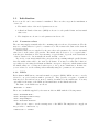
by the keyword model. Here is the standard linear regression example:
model {
for (i in 1:N) {
Y[i]
~ dnorm(mu[i], tau)
mu[i] <- alpha + beta * (x[i] - x.bar)
}
x.bar
<- mean(x)
6
alpha
beta
sigma
tau
~
~
<~
dnorm(0.0, 1.0E-4)
dnorm(0.0, 1.0E-4)
1.0/sqrt(tau)
dgamma(1.0E-3, 1.0E-3)
}
Each relation defines a node in the model in terms of other nodes that appear on the right
hand side. These are referred to as the parent nodes. Taken together, the nodes in the model
(together with the parent/child relationships represented as directed edges) form a directed
acyclic graph. The very top-level nodes in the graph, with no parents, are constant nodes,
which are defined either in the model definition (e.g. 1.0E-3), or in the data file (e.g. x[1]).
Relations can be of two types. A stochastic relation (~) defines a stochastic node, representing a random variable in the model. A deterministic relation (<-) defines a deterministic
node, the value of which is determined exactly by the values of its parents.
Nodes defined by a relation are embedded in named arrays. Array names may contain
letters, numbers, decimal points and underscores, but they must start with a letter. The
node array mu is a vector of length N containing N nodes (mu[1], . . ., mu[N]). The node
array alpha is a scalar. JAGS follows the S language convention that scalars are considered
as vectors of length 1. Hence the array alpha contains a single node alpha[1].
Deterministic nodes do not need to be embedded in node arrays. The node Y[i] could
equivalently be defined as
Y[i] ~ dnorm(alpha + beta * (x[i] - x.bar), tau)
In this version of the model definition, the node previously defined as mu[i] still exists, but
is not accessible to the user as it does not have a name. This ability to hide deterministic nodes by embedding them in other expressions underscores an important fact: only the
stochastic nodes in a model are really important. Deterministic nodes are merely a syntactically convenient way of describing the relations between, or transformations of, the stochastic
nodes.
3.1.2
Data
The data are defined in a separate file from the model definition, in the format created by
the dump() function in R. The simplest way to prepare your data is to read them into R and
then dump them. Only numeric vectors, matrices and arrays are allowed. More complex
data structures such as factors, lists and data frames cannot be parsed by JAGS nor can nonnumeric vectors. Any R attributes of the data (such as names and dimnames) are stripped
when they are read into JAGS.
The data may contain missing values, but you cannot supply partially missing values for
a multivariate node. In JAGS a node is either completely observed, or completely unobserved.
The unobserved nodes are referred to as the parameters of the model. The data file therefore
defines the parameters of the model by omission.
Here are the data for the LINE example:
‘x‘ <c(1, 2, 3, 4, 5)
#R-style comments, like this one, can be embedded in the data file
7
‘Y‘ <c(1, 3, 3, 3, 5)
‘N‘ <5
It is an error to supply a data value for a deterministic node. (See, however, section 8.0.3
on observable functions).
3.1.3
Node Array dimensions
Array declarations
JAGS allows the option of declaring the dimensions of node arrays in the model file. The
declarations consist of the keyword var (for variable) followed by a comma-separated list of
array names, with their dimensions in square brackets. The dimensions may be given in terms
of any expression of the data that returns a single integer value.
In the linear regression example, the model block could be preceded by
var x[N], Y[N], mu[N], alpha, beta, tau, sigma, x.bar;
Undeclared nodes
If a node array is not declared then JAGS has three methods of determining its size.
1. Using the data. The dimension of an undeclared node array may be inferred if it is
supplied in the data file.
2. Using the left hand side of the relations. The maximal index values on the left
hand side of a relation are taken to be the dimensions of the node array. For example,
in this case:
for (i in 1:N) {
for (j in 1:M) {
Y[i,j] ~ dnorm(mu[i,j], tau)
}
}
Y would be inferred to be an N × M matrix. Using this method, empty indices are not
allowed on the left hand side of any relation.
3. Using the dimensions of the parents If a whole node array appears on the left hand
side of a relation, then its dimensions can be inferred from the dimensions of the nodes
on the right hand side. For example, if A is known to be an N × N matrix and
B <- inverse(A)
Then B is also an N × N matrix.
8
Querying array dimensions
The JAGS compiler has two built-in functions for querying array sizes. The length() function
returns the number of elements in a node array, and the dim() function returns a vector
containing the dimensions of an array. These two functions may be used to simplify the data
preparation. For example, if Y represents a vector of observed values, then using the length()
function in a for loop:
for (i in 1:length(Y)) {
Y[i] ~ dnorm(mu[i], tau)
}
avoids the need to put a separate data value N in the file representing the length of Y.
For multi-dimensional arrays, the dim function serves a similar purpose. The dim function
returns a vector, which must be stored in an array before its elements can be accessed. For
this reason, calls to the dim function must always be in a data block (see section 8.0.4).
data {
D <- dim(Z)
}
model {
for (i in 1:D[1]) {
for (j in 1:D[2]) {
Z[i,j] <- dnorm(alpha[i] + beta[j], tau)
}
}
...
}
Clearly, the length() and dim() functions can only work if the size of the node array can be
inferred, using one of the three methods outlined above.
Note: the length() and dim() functions are different from all other functions in JAGS:
they do not act on nodes, but only on node arrays. As a consequence, an expression such as
dim(a %*% b) is syntactically incorrect.
3.2
Compilation
When a model is compiled, a graph representing the model is created in computer memory.
Compilation can fail for a number of reasons:
1. The graph contains a directed cycle. These are forbidden in JAGS.
2. A top-level parameter is undefined. Any node that is used on the right hand side of
a relation, but is not defined on the left hand side of any relation, is assumed to be a
constant node. Its value must be supplied in the data file.
3. The model uses a function or distribution that has not been defined in any of the loaded
modules.
The number of parallel chains to be run by JAGS is also defined at compilation time. Each
parallel chain should produce an independent sequence of samples from the posterior distribution. By default, JAGS only runs a single chain.
9
3.3
Initialization
Before a model can be run, it must be initialized. There are three steps in the initialization
of a model:
1. The initial values of the model parameters are set.
2. A Random Number Generator (RNG) is chosen for each parallel chain, and its initial
value is set.
3. The Samplers are chosen for each parameter in the model.
3.3.1
Parameter values
The user may supply an initial value file containing values for the model parameters. The file
may not contain values for logical or constant nodes. The format is the same as the data file
(see section 3.1.2).
If initial values are not supplied by the user, then each parameter chooses its own initial
value based on the values of its parents. The initial value is chosen to be a “typical value”
from the prior distribution. The exact meaning of “typical value” depends on the distribution
of the stochastic node, but is usually the mean, median, or mode.
If you rely on automatic initial value generation and are running multiple parallel chains,
then the initial values will be the same in all chains. You may not want this behaviour,
especially if you are using the Gelman and Rubin convergence diagnostic, which assumes that
the initial values are over-dispersed with respect to the posterior distribution. In this case,
you are advised to set the starting values manually using the ”parameters in” statement.
3.3.2
RNGs
Each chain in JAGS has its own random number generator (RNG). RNGs are more correctly
referred to as pseudo-random number generators. They generate a sequence of numbers
that merely looks random but is, in fact, entirely determined by the initial state. You may
optionally set the name of the RNG and its initial state in the initial values file.
The name of the RNG is set as follows.
.RNG.name <- "name"
There are four RNGs supplied by the base module in JAGS with the following names:
"base::Wichmann-Hill"
"base::Marsaglia-Multicarry"
"base::Super-Duper"
"base::Mersenne-Twister"
There are two ways to set the starting state of the RNG. The simplest is to supply an
integer value to .RNG.seed, e.g.
".RNG.seed" <- 314159
10
The second is way to save the state of the RNG from one JAGS session (see the “PARAMETERS TO” statement, section 4.1.12) and use this as the initial state of a new chain. The
state of any RNG in JAGS can be saved and loaded as an integer vector with the name
.RNG.state. For example,
".RNG.state" <- as.integer(c(20899,10892,29018))
is a valid state for the Marsaglia-Multicarry generator. You cannot supply an arbitrary integer
to .RNG.state. Both the length of the vector and the permitted values of its elements are
determined by the class of the RNG. The only safe way to use .RNG.state is to re-use a
previously saved state.
If no RNG names are supplied, then RNGs will be chosen automatically so that each
chain has its own independent random number stream. The exact behaviour depends on
which modules are loaded. The base module uses the four generators listed above for the
first four chains, then recycles them with different seeds for the next four chains, and so on.
By default, JAGS bases the initial state on the time stamp. This means that, when a
model is re-run, it generates an independent set of samples. If you want your model run to
be reproducible, you must explicitly set the .RNG.seed for each chain.
3.3.3
Samplers
A Sampler is an object that acts on a set of parameters and updates them from one iteration
to the next. During initialization of the model, Samplers are chosen automatically for all
parameters.
The Model holds an internal list of Sampler Factory objects, which inspect the graph,
recognize sets of parameters that can be updated with specific methods, and generate Sampler
objects for them. The list of Sampler Factories is traversed in order, starting with sampling
methods that are efficient, but limited to certain specific model structures and ending with
the most generic, possibly inefficient, methods. If no suitable Sampler can be generated for
one of the model parameters, an error message is generated.
The user has no direct control over the process of choosing Samplers. However, you may
indirectly control the process by loading a module that defines a new Sampler Factory. The
module will insert the new Sampler Factory at the beginning of the list, where it will be
queried before all of the other Sampler Factories. You can also optionally turn on and off
sampler factories using the “SET FACTORY” command. See 4.1.18.
A report on the samplers chosen by the model, and the stochastic nodes they act on, can
be generated using the “SAMPLERS TO” command. See section 4.1.13.
3.4
Adaptation and burn-in
In theory, output from an MCMC sampler converges to the target distribution (i.e. the
posterior distribution of the model parameters) in the limit as the number of iterations tends
to infinity. In practice, all MCMC runs are finite. By convention, the MCMC output is
divided into two parts: an initial “burn-in” period, which is discarded, and the remainder
of the run, in which the output is considered to have converged (sufficiently close) to the
target distribution. Samples from the second part are used to create approximate summary
statistics for the target distribution.
11
By default, JAGS keeps only the current value of each node in the model, unless a monitor
has been defined for that node. The burn-in period of a JAGS run is therefore the interval
between model initialization and the creation of the first monitor.
When a model is initialized, it is in adaptive mode, meaning that the Samplers used by the
model may modify their behaviour for increased efficiency. Since this adaptation may depend
on the entire sample history, the sequence generated by an adapting sampler is no longer
a Markov chain, and is not guaranteed to converge to the target distribution. Therefore,
adaptive mode must be turned off at some point during burn-in, and a sufficient number of
iterations must take place after the adaptive phase to ensure convergence.
By default, adaptive mode is turned off half way through first update of a JAGS model,
although the user may also control the length of the adaptive phase directly. All samplers have
a built in test to determine whether they have converged to their optimal sampling behaviour.
If any sampler fails this validation test, a warning will be printed. To ensure optimal sampling
behaviour, the model should be run again from scratch using a longer adaptation period.
3.5
Monitoring
A monitor in JAGS is an object that records sampled values. The simplest monitor is a trace
monitor, which stores the sampled value of a node at each iteration.
JAGS cannot monitor a node unless it has been defined in the model file. For vector- or
array-valued nodes, this means that every element must be defined. Here is an example of a
simple for loop that only defines elements 2 to N of theta
for (i in 2:N) {
theta[i] ~ dnorm(0,1);
}
Unless theta[1] is defined somewhere else in the model file, the multivariate node theta
is undefined and therefore it will not be possible to monitor theta as a whole. In such cases
you can request each element separately , e.g. theta[2], theta[3], etc., or request a subset
that is fully defined, e.g. theta[2:6].
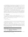
Monitors can be classified according to whether they pool values over iterations and
whether they pool values over parallel chains (The standard trace monitor does neither).
When monitor values are written out to file using the CODA command, the output files created depend on the pooling of the monitor, as shown in table 3.1. By default, all of these files
have the prefix CODA, but this may be changed to any other name using the “stem” option
to the CODA command (See 4.1.9).
Pool
iterations
no
no
yes
yes
Pool
chains
no
yes
no
yes
Output files
CODAindex.txt, CODAchain1.txt, ... CODAchainN.txt
CODAindex0.txt, CODAchain0.txt
CODAtable1.txt, ... CODAtableN.txt
CODAtable0.txt
Table 3.1: Output files created by the CODA command depending on whether a monitor
pools its values over chains or over iterations
12
The standard CODA format for monitors that do not pool values over iterations is to
create an index file and one or more output files. The index file is has three columns with,
one each line,
1. A string giving the name of the (scalar) value being recorded
2. The first line in the output file(s)
3. The last line in the output file(s)
The output file(s) contain two columns:
1. The iteration number
2. The value at that iteration
Some monitors pool values over iterations. For example a mean monitor may record only
the sample mean of a node, without keeping the individual values from each iteration. Such
monitors are written out to a table file with two columns:
1. A string giving the name of the (scalar) value being recorded
2. The value (pooled over all iterations)
13
Chapter 4
Running JAGS
JAGS has a command line interface. To invoke jags interactively, simply type jags at the
shell prompt on Unix, or the Windows command prompt on Windows. To invoke JAGS with
a script file, type
jags <script file>
A typical script file has the following commands:
model in "line.bug"
# Read model file
data in "line-data.R"
# Read data in from file
compile, nchains(2)
# Compile a model with two parallel chains
parameters in "line-inits.R" # Read initial values from file
initialize
# Initialize the model
update 1000
# Adaptation (if necessary) and burnin for 1000 iterations
monitor alpha
# Set trace monitor for node alpha ...
monitor beta
# ... and beta
monitor sigma
# ... and sigma
update 10000
# Update model for 10000 iterations
coda *
# All monitored values are written out to file
More examples can be found in the file classic-bugs.tar.gz which is available from the
JAGS web page.
Output from JAGS is printed to the standard output, even when a script file is being used.
The JAGS interface is designed to be forgiving. It will print a warning message if you make
a mistake, but otherwise try to keep going. This may create a cascade of error messages, of
which only the first is informative.
4.1
Scripting commands
JAGS has a simple set of scripting commands with a syntax loosely based on Stata. Commands
are shown below preceded by a dot (.). This is the JAGS prompt. Do not type the dot in
when you are entering the commands.
C-style block comments taking the form /* ... */ can be embedded anywhere in the script
file. Additionally, you may use R-style single-line comments starting with #.
14
If a scripting command takes a file name, then the name may be optionally enclosed in
quotes. Quotes are required when the file name contains space, or any character which is not
alphanumeric, or one of the following: _, -, ., /, \.
In the descriptions below, angular brackets <>, and the text inside them, represents a
parameter that should be replaced with the correct value by you. Anything inside square
brackets [] is optional. Do not type the square brackets if you wish to use an option.
4.1.1
MODEL IN
. model in <file>
Checks the syntactic correctness of the model description in file and reads it into memory.
The next compilation statement will compile this model.
See also: MODEL CLEAR (4.1.19)
4.1.2
DATA IN
. data in <file>
JAGS keeps an internal data table containing the values of observed nodes inside each node
array. The DATA IN statement reads data from a file into this data table.
Several data statements may be used to read in data from more than one file. If two data
files contain data for the same node array, the second set of values will overwrite the first,
and a warning will be printed.
See also: DATA TO (4.1.11).
4.1.3
COMPILE
. compile [, nchains(<n>)]
Compiles the model using the information provided in the preceding model and data statements. By default, a single Markov chain is created for the model, but if the nchains option
is given, then n chains are created
Following the compilation of the model, further DATA IN statements are legal, but have
no effect. A new model statement, on the other hand, will replace the current model.
4.1.4
PARAMETERS IN
. parameters in <file> [, chain(<n>)]
Reads the values in file and writes them to the corresponding parameters in chain n. The
file has the same format as the one in the DATA IN statement. The chain option may be
omitted, in which case the parameter values in all chains are set to the same value.
The PARAMETERS IN statement may be used before a model has been initialized. You
may only supply the values of unobserved stochastic nodes in the parameters file. Logical
nodes and constant nodes are forbidden.
See also: PARAMETERS TO (4.1.12)
15
4.1.5
INITIALIZE
. initialize
Initializes the model using the previously supplied data and parameter values supplied for
each chain.
4.1.6
UPDATE
. update <n> [,by(<m>)]
Updates the model by n iterations.
The first UPDATE statement turns off adaptive mode for all samplers in the model after
n/2 iterations. A warning is printed if adaptation is incomplete. Incomplete adaptation
means that the mixing of the Markov chain is not optimal. It is still possible to continue with
a model that has not completely adapted, but it may be preferable to run the model again
with a longer adaptation phase, starting from the MODEL IN statement.
A progress bar is printed on the standard output consisting of 50 asterisks. If the by
option is supplied, a new asterisk is printed every m iterations. If this entails more than 50
asterisks, the progress bar will be wrapped over several lines. If m is zero, the printing of the
progress bar is suppressed.
4.1.7
ADAPT
. adapt <n> [,by(<m>)]
Updates the model by n iterations and then turns of adaptive mode.
Use this instead of the first UPDATE statement if you want explicit control over the
length of the adaptive sampling phase.
4.1.8
MONITOR
In JAGS, a monitor is an object that calculates summary statistics from a model. The most
commonly used monitor simply records the value of a single node at each iteration. This is
called a “trace” monitor.
. monitor <varname> [, thin(n)] [type(<montype>)]
The thin option sets the thinning interval of the monitor so that it will only record every nth
value. The thin option selects the type of monitor to create. The default type is trace.
More complex monitors can be defined that do additional calculations. For example,
the dic module defines a “deviance” monitor that records the deviance of the model at
each iteration, and a “pD” monitor that calculates an estimate of the effective number of
parameters on the model [11].
. monitor clear <varname> [type(<montype>)]
Clears the monitor of the given type associated with variable <varname>.
16
4.1.9
CODA
. coda <varname> [, stem(<filename>)]
If the named node has a trace monitor, this dumps the monitored values of to files CODAindex.txt,
CODAindex1.out, CODAindex2.txt, . . . in a form that can be read by the coda package of R.
The stem option may be used to modify the prefix from “CODA” to another string. The
wild-card character “*” may be used to dump all monitored nodes
4.1.10
EXIT
. exit
Exits JAGS. JAGS will also exit when it reads an end-of-file character.
4.1.11
DATA TO
. data to <filename>
Writes the data (i.e. the values of the observed nodes) to a file in the R dump format. The
same file can be used in a DATA IN statement for a subsequent model.
See also: DATA IN (4.1.2)
4.1.12
PARAMETERS TO
. parameters to <file> [, chain(<n>)]
Writes the current parameter values (i.e. the values of the unobserved stochastic nodes) in
chain <n> to a file in R dump format. The name and current state of the RNG for chain
<n> is also dumped to the file. The same file can be used as input in a PARAMETERS IN
statement in a subsequent run.
See also: PARAMETERS IN (4.1.4)
4.1.13
SAMPLERS TO
. samplers to <file>
Writes out a summary of the samplers to the given file. The output appears in three tabseparated columns, with one row for each sampled node
• The index number of the sampler (starting with 1). The index number gives the order
in which Samplers are updated at each iteration.
• The name of the sampler, matching the index number
• The name of the sampled node.
If a Sampler updates multiple nodes then it is represented by multiple rows with the same
index number.
17
4.1.14
LOAD
. load <module>
Loads a module into JAGS (see chapter 5). Loading a module does not affect any previously
initialized models, but will affect the future behaviour of the compiler and model initialization.
4.1.15
UNLOAD
. unload <module>
Unloads a module. Currently initialized models are unaffected, but the functions, distribution,
and factory objects in the model will not be accessible to future models.
4.1.16
LIST MODULES
. list modules
Prints a list of the currently loaded modules.
4.1.17
LIST FACTORIES
. list factories, type(<factype>)
List the currently loaded factory objects and whether or not they are active. The type option
must be given, and the three possible values of <factype> are sampler, monitor, and rng.
4.1.18
SET FACTORY
. set factory "<facname>" <status>, type(<factype>)
Sets the status of a factor object. The possible values of <status> are on and off. Possible
factory names are given from the LIST MODULES command.
4.1.19
MODEL CLEAR
. model clear
Clears the current model. The data table (see section 4.1.2) remains intact
4.1.20
Print Working Directory (PWD)
. pwd
Prints the name of the current working directory. This is where JAGS will look for files when
the file name is given without a full path, e.g. "mymodel.bug".
4.1.21
Change Directory (CD)
. cd <dirname>
Changes the working directory to <dirname>
18
4.1.22
Directory list (DIR)
. dir
Lists the files in the current working directory.
4.1.23
RUN
. run <cmdfile>
Opens the file <cmdfile> and reads further scripting commands until the end of the file. Note
that if the file contains an EXIT statement, then the JAGS session will terminate.
4.2
Errors
There are two kinds of errors in JAGS: runtime errors, which are due to mistakes in the model
specification, and logic errors which are internal errors in the JAGS program.
Logic errors are generally created in the lower-level parts of the JAGS library, where it is
not possible to give an informative error message. The upper layers of the JAGS program are
supposed to catch such errors before they occur, and return a useful error message that will
help you diagnose the problem. Inevitably, some errors slip through. Hence, if you get a logic
error, there is probably an error in your input to JAGS, although it may not be obvious what
it is. Please send a bug report (see “Feedback” below) whenever you get a logic error.
Error messages may also be generated when parsing files (model files, data files, command
files). The error messages generated in this case are created automatically by the program
bison. They generally take the form “syntax error, unexpected FOO, expecting BAR” and
are not always abundantly clear.
If a model compiles and initializes correctly, but an error occurs during updating, then
the current state of the model will be dumped to a file named jags.dumpN.R where N is the
chain number. You should then load the dumped data into R to inspect the state of each
chain when the error occurred.
19
Chapter 5
Modules
The JAGS library is distributed along with certain dynamically loadable modules that extend
its functionality. A module can define new objects of the following classes:
1. functions and distributions, the basic building blocks of the BUGS language.
2. samplers, the objects which update the parameters of the model at each iteration, and
sampler factories, the objects that create new samplers for specific model structures.
If the module defines a new distribution, then it will typically also define a new sampler
for that distribution.
3. monitors, the objects that record sampled values for later analysis, and monitor
factories that create them.
4. random number generators, the objects that drive the MCMC algorithm and RNG
factories that create them.
The base module and the bugs module are loaded automatically at start time. Others
may be loaded by the user.
5.1
The base module
The base module supply the base functionality for the JAGS library to function correctly. It
is loaded first by default.
5.1.1
Base Samplers
The base module defines samplers that use highly generic update methods. These sampling
methods only require basic information about the stochastic nodes they sample. Conversely,
they may not be fully efficient.
Three samplers are currently defined:
1. The Finite sampler can sample a discrete-valued node with fixed support of less than
20 possible values. The node must not be bounded using the T(,) construct
2. The Real Slice Sampler can sample any scalar real-valued stochastic node.
3. The Discrete Slice Sampler can sample any scalar discrete-valued stochastic node.
20
5.1.2
Base RNGs
The base module defines four RNGs, taken directly from R, with the following names:
1. "base::Wichmann-Hill"
2. "base::Marsaglia-Multicarry"
3. "base::Super-Duper"
4. "base::Mersenne-Twister"
A single RNG factory object is also defined by the base module which will supply these
RNGs for chains 1 to 4 respectively, if “RNG.name” is not specified in the initial values file.
All chains generated by the base RNG factory are initialized using the current time stamp.
If you have more than four parallel chains, then the base module will recycle the same for
RNGs, but using different seeds. If you want many parallel chains then you may wish to load
the lecuyer module.
5.1.3
Base Monitors
The base module defines the TraceMonitor class (type “trace”). This is the monitor class
that simply records the current value of the node at each iteration.
5.2
The bugs module
The bugs module defines some of the functions and distributions from WinBUGS. These are
described in more detail in sections 6 and 7. The bugs module also defines conjugate samplers
for efficient Gibbs sampling.
5.3
The mix module
The mix module defines a novel distribution dnormmix(mu,tau,pi) representing a finite mixture of normal distributions. In the parameterization of the dnormmix distribution, µ, τ , and
π are vectors of the same length, and the density of y ~ dnormmix(mu, tau, pi) is
f (y|µ, τ, π) =
X
1
1
πi τi2 φ(τi2 (y − µi ))
i
where φ() is the probability density function of a standard normal distribution.
The mix module also defines a sampler that is designed to act on finite normal mixtures.
It uses tempered transitions to jump between distant modes of the multi-modal posterior
distribution generated by such models [8, 2]. The tempered transition method is computationally very expensive. If you want to use the dnormmix distribution but do not care about
label switching, then you can disable the tempered transition sampler with
set factory "mix::TemperedMix" off, type(sampler)
21
5.4
The dic module
The dic module defines new monitor classes for Bayesian model criticism using deviancebased measures.
5.4.1
The deviance monitor
The deviance monitor records the deviance of the model (i.e. the sum of the deviances of all
the observed stochastic nodes) at each iteration. The command
monitor deviance
will create a deviance monitor unless you have defined a node called “deviance” in your model.
In this case, you will get a trace monitor for your deviance node.
5.4.2
The pD monitor
The pD monitor is used to estimate the effective number of parameters (pD ) of the model [11].
It requires at least two parallel chains in the model, but calculates a single estimate of pD
across all chains [9]. A pD monitor can be created using the command:
monitor pD
Like the deviance monitor, however, if you have defined a node called “pD” in your model
then this will take precedence, and you will get a trace monitor for your pD node.
Since the pD monitor pools its value across all chains, its values will be written out to the
index file “CODAindex0.txt” and output file “CODAoutput0.txt” when you use the CODA
command.
The effective number of
Pparameters is the sum of separate contributions from all observed
stochastic nodes: pD =
i pDi . There is also a monitor that stores the sample mean of
pDi . These statistics may be used as influence diagnostics [11]. The mean monitor for pDi is
created with:
monitor pD, type(mean)
Its values can be written out to a file “PDtable0.txt” with
coda pD, type(mean) stem(PD)
5.4.3
The popt monitor
The popt monitor works exactly like the mean monitor for pD , but records contributions
to
P
the optimism of the expected deviance (popti ). The total optimism popt = i popti can be
added to the mean deviance to give the penalized expected deviance [10].
The mean monitor for popti is created with
monitor popt, type(mean)
Its values can be written out to a file “POPTtable0.txt” with
coda popt, type(mean) step(POPT)
22
Under asymptotically favourable conditions in which pDi 1∀i,
popt ≈ 2pD
For generalized linear models, a better approximation is
popt ≈
n
X
i=1
pDi
1 − pDi
The popt monitor uses importance weights to estimate popt . The resulting estimates may
be numerically unstable when pDi is not small. This typically occurs in random-effects models,
so it is recommended to use caution with the popt until I can find a better way of estimating
popti .
5.5
The msm module
The msm module defines the matrix exponential function mexp and the multi-state distribution
dmstate which describes the transitions between observed states in continuous-time multistate Markov transition models.
5.6
The glm module
The glm module implements samplers for efficient updating of generalized linear mixed models. The fundamental idea is to do block updating of the parameters in the linear predictor.
The glm module is built on top of the Csparse sparse matrix library [3] which allows updating
of both fixed and random effects in the same block. Currently, the methods only work on
parameters that have a normal prior distribution.
Some of the samplers are based in the idea of introducing latent normal variables that
reduce the GLM to a linear model. This idea was introduced by Albert and Chib [1] for probit
regression with a binary outcome, and was later refined and extended to logistic regression
with binary outcomes by Holmes and Held [6]. Another approach, auxiliary mixture sampling, was developed by Frühwirth-Schnatter et al [4] and is used for more general Poisson
regression and logistic regression models with binomial outcomes. Gamerman [5] proposed
a stochastic version of the iteratively weighted least squares algorithm for GLMs, which is
also implemented in the glm module. However the IWLS sampler tends to break down when
there are many random effects in the model. It uses Metropolis-Hastings updates, and the
acceptance probability may be very small under these circumstances.
Block updating in GLMMs frees the user from the need to center predictor variables, like
this:
y[i] ~ dnorm(mu[i], tau)
mu[i] <- alpha + beta * (x[i] - mean(x))
The second line can simply be written
mu[i] <- alpha + beta * x[i]
without affecting the mixing of the Markov chain.
23
Chapter 6
Functions
Functions allow deterministic nodes to be defined using the <- (“gets”) operator. Most of the
functions in JAGS are scalar functions taking scalar arguments. However, JAGS also allows
arbitrary vector- and array-valued functions, such as the matrix multiplication operator %*%
and the transpose function t() defined in the bugs module, and the matrix exponential
function mexp() defined in the msm module. JAGS also uses an enriched dialect of the BUGS
language with a number of operators that are used in the S language.
Scalar functions taking scalar arguments are automatically vectorized. They can also be
called when the arguments are arrays with conforming dimensions, or scalars. So, for example,
the scalar c can be added to the matrix A using
B <- A + c
instead of the more verbose form
D <- dim(A)
for (i in 1:D[1])
for (j in 1:D[2]) {
B[i,j] <- A[i,j] + c
}
}
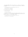
6.1
Base functions
The functions defined by the base module all appear as infix or prefix operators. The syntax
of these operators is built into the JAGS parser. They are therefore considered part of the
modelling language. Table 6.1 lists them in reverse order of precedence.
Logical operators convert numerical arguments to logical values: zero arguments are converted to FALSE and non-zero arguments to TRUE. Logical and comparison operators return
the value 1 if the result is TRUE and 0 if the result is FALSE. Comparison operators are
non-associative: the expression x < y < z, for example, is syntactically incorrect.
The %special% function is an exception in table 6.1. It is not a function defined by the
base module, but is a place-holder for any function with a name starting and ending with
the character “%” Such functions are automatically recognized as infix operators by the JAGS
model parser, with precedence defined by table 6.1.
24
Type
Logical
operators
Comparison
operators
Arithmetic
operators
Power function
Usage
x || y
x && y
!x
x > y
x >= y
x < y
x <= y
x == y
x + y
x - y
x * y
x / y
x %special% y
-x
x^y
Description
Or
And
Not
Greater than
Greater than or equal to
Less than
Less than or equal to
Equal
Addition
Subtraction
Multiplication
Division
User-defined operators
Unary minus
Table 6.1: Base functions listed in reverse order of precedence
6.2
6.2.1
Functions in the bugs module
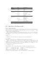
Scalar functions
Table 6.2 lists the scalar-valued functions in the bugs module that also have scalar arguments.
These functions are automatically vectorized when they are given vector, matrix, or array
arguments with conforming dimensions.
Table 6.4 lists the link functions in the bugs module. These are smooth scalar-valued functions that may be specified using an S-style replacement function notation. So, for example,
the log link
log(y) <- x
is equivalent to the more direct use of its inverse, the exponential function:
y <- exp(x)
This usage comes from the use of link functions in generalized linear models.
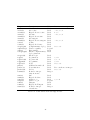
Table 6.3 shows functions to calculate the probability density, probability function, and
quantiles of some of the distributions provided by the bugs module. These functions are
parameterized in the same way as the corresponding distribution. For example, if x has a
normal distribution with mean µ and precision τ
x ~ dnorm(mu, tau)
Then the usage of the corresponding density, probability, and quantile functions is:
density.x <- dnorm(x, mu, tau)
# Density of normal distribution at x
prob.x
<- pnorm(x, mu, tau)
# P(X <= x)
quantile90.x <- qnorm(0.9, mu, tau) # 90th percentile
For details of the parameterization of the other distributions, see tables 7.1 and 7.2.
25
Usage
abs(x)
acos(x)
acosh(x)
asin(x)
asinh(x)
atan(x)
atanh(x)
cos(x)
cosh(x)
cloglog(x)
equals(x,y)
exp(x)
icloglog(x)
ilogit(x)
log(x)
logfact(x)
loggam(x)
logit(x)
phi(x)
pow(x,z)
probit(x)
round(x)
sin(x)
sinh(x)
sqrt(x)
step(x)
tan(x)
tanh(x)
trunc(x)
Description
Absolute value
Arc-cosine
Hyperbolic arc-cosine
Arc-sine
Hyperbolic arc-sine
Arc-tangent
Hyperbolic arc-tangent
Cosine
Hyperbolic Cosine
Complementary log log
Test for equality
Exponential
Inverse complementary
log log function
Inverse logit
Log function
Log factorial
Log gamma
Logit
Standard normal cdf
Power function
Probit
Round to integer
away from zero
Sine
Hyperbolic Sine
Square-root
Test for x ≥ 0
Tangent
Hyperbolic Tangent
Round to integer
towards zero
Value
Real
Real
Real
Real
Real
Real
Real
Real
Real
Real
Logical
Real
Real
Real
Real
Real
Real
Real
Real
Real
Real
Integer
Real
Real
Real
Logical
Real
Real
Integer
Restrictions on arguments
−1 < x < 1
1<x
−1 < x < 1
−1 < x < 1
0<x<1
x>0
x > −1
x>0
0<x<1
If x < 0 then z is integer
0<x<1
x >= 0
Table 6.2: Scalar functions in the bugs module
26
Distribution
Bernoulli
Beta
Binomial
Chi-square
Double exponential
Exponential
F
Gamma
Generalized gamma
Hypergeometric
Log-normal
Negative binomial
Normal
Pareto
Poisson
Student t
Weibull
Density
dbern
dbeta
dbin
dchisqr
ddexp
dexp
df
dgamma
dgengamma
dhyper
dlnorm
dnegbin
dnorm
dpar
dpois
dt
dweib
Distribution
pbern
pbeta
pbin
pchisqr
pdexp
pexp
pf
pgamma
pgengamma
phyper
plnorm
pnegbin
pnorm
ppar
ppois
pt
pweib
Quantile
qbern
qbeta
qbin
qchisqr
qdexp
qexp
qf
qgamma
qgengamma
qhyper
qlnorm
qnegbin
qnorm
qpar
qpois
qt
qweib
Table 6.3: Wrappers for the d-p-q functions from the Rmath library
Link function
cloglog(y) <- x
log(y) <- x
logit(y) <- x
probit(y) <- x
Description
Complementary log log
Log
Logit
Probit
Range
0<y<1
0<y
0<y<1
0<y<1
Inverse
y <- icloglog(x)
y <- exp(x)
y <- ilogit(x)
y <- phi(x)
Table 6.4: Link functions in the bugs module
27
Function
inprod(x1,x2)
interp.lin(e,v1,v2)
Description
Inner product
Linear Interpolation
logdet(a)
max(x1,x2,...)
mean(x)
min(x1,x2,...)
prod(x)
sum(a)
sd(a)
Log determinant
Maximum element among all arguments
Mean of elements of a
Minimum element among all arguments
Product of elements of a
Sum of elements of a
Standard deviation of elements of a
Restrictions
Dimensions of a, b conform
e scalar,
v1, v2 conforming vectors
a is a square matrix
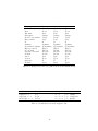
Table 6.5: Scalar-valued functions with general arguments in the bugs module
Usage
inverse(a)
mexp(a)
rank(v)
sort(v)
t(a)
a %*% b
Description
Matrix inverse
Matrix exponential
Ranks of elements of v
Elements of v in order
Transpose
Matrix multiplication
Restrictions
a is a symmetric positive definite matrix
a is a square matrix
v is a vector
v is a vector
a is a matrix
a, b conforming vector or matrices
Table 6.6: Vector- or matrix-valued functions in the bugs module
6.3
Scalar-valued functions with vector arguments
Table 6.5 lists the scalar-valued functions in the bugs module that take general arguments.
Unless otherwise stated in table 6.5, the arguments to these functions may be scalar, vector,
or higher-dimensional arrays.
The max() and min() functions work like the corresponding R functions. They take a
variable number of arguments and return the maximum/minimum element over all supplied
arguments. This usage is compatible with WinBUGS, although more general.
6.4
Vector- and array-valued functions
Table 6.6 lists vector- or matrix-valued functions in the bugs module.
The sort and rank functions behaves like their R namesakes: sort accepts a vector and
returns the same values sorted in ascending order; rank returns a vector of ranks. This is
distinct from WinBUGS, which has two scalar-valued functions rank and ranked.
28
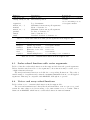
Chapter 7
Distributions
Distributions are used to define stochastic nodes using the ~ operator. The distributions
defined in the bugs module are listed in table 7.1 (real-valued distributions), 7.2 (discretevalued distributions), and 7.3 (multivariate distributions).
Some distributions have restrictions on the valid parameter values, and these are indicated
in the tables. If a Distribution is given invalid parameter values when evaluating the loglikelihood, it returns −∞. When a model is initialized, all stochastic nodes are checked to
ensure that the initial parameter values are valid for their distribution.
29
Name
Beta
Chi-square
Double
exponential
Exponential
F
Gamma
Generalized
gamma
Log-normal
Normal
Pareto
Student t
Uniform
Weibull
Usage
dbeta(a,b)
a > 0, b > 0
dchisqr(k)
k>0
ddexp(mu,tau)
τ >0
dexp(lambda)
λ>0
df(n,m)
n > 0, m > 0
dgamma(r, mu)
µ > 0, r > 0
dgen.gamma(r,mu,beta)
µ > 0, β > 0, r > 0
dlnorm(mu,tau)
τ >0
dnorm(mu,tau)
τ >0
dpar(alpha, c)
α > 0, c > 0
dt(mu,tau,k)
τ > 0, k > 0
dunif(a,b)
a<b
dweib(v, lambda)
v > 0, λ > 0
Density
− x)b−1
β(a, b)
k
−1
x 2 exp(−x/2)
k
2 2 Γ( k2 )
τ exp(−τ |x − µ|)/2
Lower
0
xa−1 (1
0
0
λ exp(−λx)
Γ( n+m
)
2
m
Γ( n
)Γ(
)
2
2
n
m
n
2
n
x 2 −1 1 +
nx −
m
(n+m)
2
0
µr xr−1 exp(−µx)
Γ(r)
0
βµβr xβr−1 exp{−(µx)β }
0
1
τ 2 x−1 exp −τ (log(x) − µ)2 /2
0
τ
2π
1
exp{−(x − µ)2 τ }
2
c
αcα x−(α+1)
Γ( k+1
)
2
Γ( k2 )
τ
kπ
Upper
1
1 n
2
1+
τ (x−µ)2
k
o− (k+1)
2
1
b−a
a
vλxv−1 exp(−λxv )
0
b
Table 7.1: Univariate real-valued distributions in the bugs module
Name
Bernoulli
Binomial
Categorical
Hypergeometric
Negative
binomial
Poisson
Usage
dbern(p)
0<p<1
dbin(p,n)
0 < p < 1, n ∈ N∗
dcat(p)
p ∈ (R+ )N
dhyper(n1,n2,m1,psi)
0 ≤ ni , 0 < m1 ≤ n+
dnegbin(p, r)
0 < p < 1, r ∈ N+
dpois(lambda)
λ>0
Density
px (1 − p)1−x
n
x
px (1 − p)n−x
Ppx
i pi
n1
x
n2
m1 −x
x+r−1
x
ψx
pr (1 − p)x
exp(−λ)λx
x!
Lower
0
Upper
1
0
n
1
N
max(0, n+ − m1 )
min(n1 , m1 )
0
0
Table 7.2: Discrete univariate distributions in the bugs module
30
Name
Dirichlet
Usage
p ~ ddirch(alpha)
αj ≥ 0
Multivariate
normal
Wishart
x ~ dmnorm(mu,Omega)
Ω positive definite
Omega ~ dwish(R,k)
R pos. def.
x ~ dmt(mu,Omega,k)
Ω pos. def.
x ~ dmulti(p, n)
P
i xi = n
Multivariate
Student t
Multinomial
Density
α −1
P
Q p j
Γ( i αi ) j j
Γ(αj )
1
|Ω| 2
exp{−(x − µ)T Ω(x − µ)/2}
2π
|Ω|(k−p−1)/2 |R|k/2 exp{−Tr(RΩ/2)}
2pk/2 Γp (k/2)
(k+p)
Γ{(k + p)/2}
1/2 1 + 1 (x − µ)T Ω(x − µ) − 2
|Ω|
k
Γ(k/2)(nπ)p/2
xj
Q p
n! j j
xj !
Table 7.3: Multivariate distributions in the bugs module
31
Chapter 8
Differences between JAGS and
WinBUGS
Although JAGS aims for the same functionality as WinBUGS, there are a number of important
differences.
8.0.1
Data format
There is no need to transpose matrices and arrays when transferring data between R and JAGS,
since JAGS stores the values of an array in “column major” order, like R and FORTRAN (i.e.
filling the left-hand index first).
If you have an S-style data file for WinBUGS and you wish to convert it for JAGS, then
use the command bugs2jags, which is supplied with the coda package.
8.0.2
Distributions
Structural zeros are allowed in the Dirichlet distribution. If
p ~ ddirch(alpha)
and some of the elements of alpha are zero, then the corresponding elements of p will be fixed
to zero.
The Multinomial (dmulti) and Categorical (dcat) distributions, which take a vector of
probabilities as a parameter, may use unnormalized probabilities. The probability vector is
normalized internally so that
pi
pi → P
j pj
8.0.3
Observable Functions
Logical nodes in the BUGS language are a convenient way of describing the relationships
between observables (constant and stochastic nodes), but are not themselves observable. You
cannot supply data values for a logical node.
This restriction can occasionally be inconvenient, as there are important cases where the
data are a deterministic function of unobserved variables. Two important examples are
32
1. Censored data, which commonly occurs in survival analysis. In the most general case,
we know that unobserved failure time T lies in the interval (L, U ].
2. Aggregate data when we observe the sum of two or more unobserved variables.
JAGS contains two novel distributions to handle these situations.
1. The dinterval distribution represents interval-censored data. It has two parameters:
t the original continuous variable, and c[], a vector of cut points of length M , say. If X
∼ dinterval(t, c) then
X=0
X=m
X=M
if
if
if
t ≤ c[1]
c[m] < t ≤ c[m + 1] for 1 ≤ m < M
c[M ] < t.
2. The dsum distribution represents the sum of two or more variables. It takes a variable
number of parameters. If Y ∼ dsum(x1,x2,x3) then Y = x1 + x2 + x3.
These distributions exist to give a likelihood to data that is, in fact, a deterministic function
of the parameters. The relation
Y ~ dsum(x1, x2)
is logically equivalent to
Y <- x1 + x2
But the latter form does not create a contribution to the likelihood, and does not allow you
to define Y as data. The likelihood function is trivial: it is 1 if the parameters are consistent
with the data and 0 otherwise. The dsum distribution also requires a special sampler, which
can currently only handle the case where the parameters of dsum are unobserved stochastic
nodes, and where the parameters are either all discrete-valued or all continuous-valued. A
node cannot be subject to more than one dsum constraint.
8.0.4
Data transformations
JAGS allows data transformations, but the syntax is different from BUGS. BUGS allows you
to put a stochastic node twice on the left hand side of a relation, as in this example taken
from the manual
for (i in 1:N) {
z[i] <- sqrt(y[i])
z[i] ~ dnorm(mu, tau)
}
This is forbidden in JAGS. You must put data transformations in a separate block of relations
preceded by the keyword data:
data {
for (i in 1:N) {
z[i] <- sqrt(y[i])
}
33
}
model {
for (i in 1:N) {
z[i] ~ dnorm(mu, tau)
}
...
}
This syntax preserves the declarative nature of the BUGS language. In effect, the data block
defines a distinct model, which describes how the data is generated. Each node in this model
is forward-sampled once, and then the node values are read back into the data table. The
data block is not limited to logical relations, but may also include stochastic relations. You
may therefore use it in simulations, generating data from a stochastic model that is different
from the one used to analyse the data in the model statement.
This example shows a simple location-scale problem in which the “true” values of the
parameters mu and tau are generated from a given prior in the data block, and the generated
data is analyzed in the model block.
data {
for (i in 1:N) {
y[i] ~ dnorm(mu.true, tau.true)
}
mu.true ~ dnorm(0,1);
tau.true ~ dgamma(1,3);
}
model {
for (i in 1:N) {
y[i] ~ dnorm(mu, tau)
}
mu ~ dnorm(0, 1.0E-3)
tau ~ dgamma(1.0E-3, 1.0E-3)
}
Beware, however, that every node in the data statement will be considered as data in the subsequent model statement. This example, although superficially similar, has a quite different
interpretation.
data {
for (i in 1:N) {
y[i] ~ dnorm(mu, tau)
}
mu ~ dnorm(0,1);
tau ~ dgamma(1,3);
}
model {
for (i in 1:N) {
y[i] ~ dnorm(mu, tau)
}
34
mu ~ dnorm(0, 1.0E-3)
tau ~ dgamma(1.0E-3, 1.0E-3)
}
Since the names mu and tau are used in both data and model blocks, these nodes will be
considered as observed in the model and their values will be fixed at those values generated
in the data block.
8.0.5
Directed cycles
Directed cycles are forbidden in JAGS. There are two important instances where directed
cycles are used in BUGS.
• Defining autoregressive priors
• Defining ordered priors
For the first case, the GeoBUGS extension to WinBUGS provides some convenient ways of
defining autoregressive priors. These should be available in a future version of JAGS.
8.0.6
Censoring, truncation and prior ordering
These are three, closely related issues that are all handled using the I(,) construct in BUGS.
Censoring occurs when a variable X is not observed directly, but is observed only to lie
in the range (L, U ]. Censoring is an a posteriori restriction of the data, and is represented in
WinBUGS by the I(,) construct, e.g.
X ~ dnorm(theta, tau) I(L,U)
where L and U are constant nodes.
Truncation occurs when a variable is known a priori to lie in a certain range. Although
BUGS has no construct for representing truncated variables, it turns out that there is no
difference between censoring and truncation for top-level parameters (i.e. variables with no
unobserved parents). Hence, for example, this
theta ~ dnorm(0, 1.0E-3) I(0, )
is a perfectly valid way to describe a parameter θ with a half-normal prior distribution.
Prior ordering occurs when a vector of nodes is known a priori to be strictly increasing
or decreasing. It can be represented in WinBUGS with symmetric I(, ) constructs, e.g.
X[1] ~ dnorm(0, 1.0E-3) I(,X[2])
X[2] ~ dnorm(0, 1.0E-3) I(X[1],)
ensures that X[1] ≤ X[2].
JAGS makes an attempt to separate these three concepts.
Censoring is handled in JAGS using the new distribution dinterval (section 8.0.3). This
can be illustrated with a survival analysis example. A right-censored survival time ti with a
Weibull distribution is described in WinBUGS as follows:
t[i] ~ dweib(r, mu[i]) I(c[i], )
35
where ti is unobserved if ti > ci . In JAGS this becomes
is.censored[i] ~ dinterval(t[i], c[i])
t[i] ~ dweib(r, mu[i])
where is.censored[i] is an indicator variable that takes the value 1 if ti is censored and 0
otherwise. See the MICE and KIDNEY examples in the “classic bugs” set of examples.
Truncation is represented in JAGS using the T(,) construct, which has the same syntax
as the I(,) construct in WinBUGS, but has a different interpretation. If
X ~ dfoo(theta) T(L,U)
then a priori X is known to lie between L and U . This generates a likelihood
p(x | θ)
P (L ≤ X ≤ U | θ)
if L ≤ X ≤ U and zero otherwise, where p(x | θ) is the density of X given θ according
to the distribution foo. Note that calculation of the denominator may be computationally
expensive.
Prior ordering of top-level parameters in the model can be achieved using the sort function, which sorts a vector in ascending order.
Symmetric truncation relations like this
alpha[1] ~ dnorm(0, 1.0E-3) I(,alpha[2])
alpha[2] ~ dnorm(0, 1.0E-3) I(alpha[1],alpha[3])
alpha[3] ~ dnorm(0, 1.0E-3) I(alpha[2],)
Should be replaced by this
for (i in 1:3) {
alpha0[i] ~ dnorm(0, 1.0E-3)
}
alpha[1:3] <- sort(alpha0)
36
Chapter 9
Feedback
Please send feedback to martyn_plummer@users.sourceforge.net. I am particularly interested in the following problems:
• Crashes, including both segmentation faults and uncaught exceptions.
• Incomprehensible error messages
• Models that should compile, but don’t
• Output that cannot be validated against WinBUGS
• Documentation erors
If you want to send a bug report, it must be reproducible. Send the model file, the data
file, the initial value file and a script file that will reproduce the problem. Describe what you
think should happen, and what did happen.
37
Chapter 10
Acknowledgments
Many thanks to the BUGS development team, without whom JAGS would not exist. Thanks
also to Simon Frost for pioneering JAGS on Windows and Bill Northcott for getting JAGS
on Mac OS X to work. Kostas Oikonomou found many bugs while getting JAGS to work
on Solaris using Sun development tools and libraries. Bettina Gruen, Chris Jackson, Greg
Ridgeway and Geoff Evans also provided useful feedback. Special thanks to Jean-Baptiste
Denis who has been very diligent in providing feedback on JAGS.
Testing of JAGS on IRIX 6.5 was carried out on Helix Systems at the National Institutes
of Health, Bethesda, MD (http://helix.nih.gov).
38
Bibliography
[1] James Albert and Siddharta Chib. Bayesian analysis of binary and polychotomous response data. Journal of the American Statistical Association, 88:669–679, 1993.
[2] Gilles Celeux, Merrilee Hurn, and Christian P. Robert. Computational and inferential
difficulties with mixture posterior distributions. Journal of the American Statistical
Association, 95:957–970, 1999.
[3] Timothy A Davis. Direct Methods for Sparse Linear Systems. SIAM, 2006.
[4] Sylvia Frühwirth-Schnatter, Rudolf Frühwirth, Leonhard Held, and Håvard Rue. Improved auxiliary mixture sampling for hierarchical models of non-gaussian data. Statistics
and Computing, 19(4):479–492, 2009.
[5] Dani Gamerman. Efficient sampling from the posterior distribution in generalized linear
mixed models. Statistics and Computing, 7:57–68, 1997.
[6] Chris Holmes and Leonard Held. Bayesian auxiliary variable models for binary and
multinomial regression. Bayesian Analysis, 1(1):145–168, 2006.
[7] P. L’Ecuyer, R. Simard, E. J. Chen, and W. D. Kelton. An object-oriented randomnumber package with many long streams and substreams. Operations Research,
50(6):1073–1075, 2002.
[8] Radford Neal. Sampling from multimodal distributions using tempered transitions.
Statistics and Computing, 6:353–366, 1994.
[9] M Plummer. Discussion of the paper by Spiegelhalter et al. Journal of the Royal Statistical Society Series B, 64:620, 2002.
[10] M Plummer. Penalized loss functions for Bayesian model comparison. Biostatistics,
9(3):523–539, 2008.
[11] DJ Spiegelhalter, NG Best, BP Carlin, and A van der Linde. Bayesian measures of model
complexity and fit (with discussion). Journal of the Royal Statistical Societey Series B,
64:583–639, 2002.
39