1
Department of Health Science and Technology
May 2008
System to Monitor the Level of Activity
of People with Severe Dementia
Treated with Music Therapy
4th semester group 471
Mike Thagaard Hagelskjær
Ann-Sofie Holm Henriksen
Carina Jensen
Lasse Sohrt-Petersen
Steffen Vangsgaard
Department of Health Science and Technology
Fredrik Bajersvej 7
9220 Aalborg Øst
Denmark
Title:
System to Monitor the Level of
Activity of People with Severe Dementia Treated with Music Therapy
Topic:
Processing of Biological Signals
Project period:
4. semester, spring 2008
Project group:
ST4 471
Participants:
Mike Thagaard Hagelskjær
Ann-Sofie Holm Henriksen
Carina Jensen
Lasse Sohrt-Petersen
Steffen Vangsgaard
Supervisor:
Erika G. Spaich
Copies: 8
Pages: 135
Appendices: 5
Finished:
30. May 2008
Music therapists claim that music therapy
has a beneficial effect on the wandering behavior of patients suffering from frontotemporal dementia. This assertion is not verified by quantitative documentation.
This project deals with the design and
implementation of a system to measure
the activity level of the patients. In the
project, there has been used a micro controller, which is programmed to record and
filter the signal from an accelerometer and
transmit it to a PC, where the data is analysed and visualised. The system is compact and intended to be placed on the ankle
of the patient.
With the system it is possible to detect the
gait events: heel strike and toe off, thus determining the swing-stance ratio. The user
of the system can manually compare data
before, during and after a music therapy
session, to see the changes in the gait.
The system has not been verified with patients suffering from frontotemporal dementia, but has been tested on a healthy
subject. The system fulfilled the technical
and functional specifications, which means
that the system is capable of measuring the
activity level.
There is free access to the contest of the report; though no reference publications without the authors agreement is accepted.
v
Preface
This report has been made by group 471, 4th semester at the Department of Health Science
and Technology, at Aalborg University. The project period lasted from the 4th of February to
the 30th of May 2008. The main theme of the semester is “Processing of Biological Signals”.
In the project period, methods to collect, process and present the signals collected from the
body in preparation for diagnosing, treating or rehabilitation, is studied.
The target group of the project is students and supervisors at the Department of Health
Science and Technology, at Aalborg University, and other interested. The group would like
to direct special thanks to John Hansen, Strahinja Dosen and Jan Stavnshøj for technical
support. Furthermore, the group would like to direct special thanks to music therapist Hanne
Mette Ochsner Ridder for participating in the interview.
Reader instructions
The project has been structured by a problem based method that consist of three parts:
• Problem Analysis
• Problem Solving
• Summary
In the end of the report, appendices are represented. The appendices are composed by
the group and contain further explanations about selected topics. A CD is attached to the
report and contains the complete code for the micro controllers and the report in .pdf format.
Sources are structured by the Vancouver method, where [1] refers to [1] in the bibliography.
When the source reference is referred before a period, the source reference only refers to the
concerned sentence. If the source reference is after a period, the source reference refers to
the section.
Figures, equations and tables are consecutively enumerated in every chapter with captions
and source references.
The following abbreviations will be used throughout the report:
• µC - Meaning micro controller
• AP - Meaning Access Point
• ED - Meaning End Device
Mike Thagaard Hagelskjær
Ann-Sofie Holm Henriksen
Carina Jensen
Lasse Sohrt-Petersen
Steffen Vangsgaard
Contents
1 Introduction
1
I
3
Problem Analysis
2 Method for Problem Analysis
5
3 Dementia
3.1 Dementia in General . . . . . . . . . . . . . . . . . . . . . . . . . . . . . . . .
3.2 Frontotemporal Dementia . . . . . . . . . . . . . . . . . . . . . . . . . . . . .
7
7
8
4 Music Therapy
11
4.1 Music Therapy in General . . . . . . . . . . . . . . . . . . . . . . . . . . . . . 11
4.2 Music Therapy and Dementia . . . . . . . . . . . . . . . . . . . . . . . . . . . 11
5 Problem Statement
13
5.1 Synthesis of Problem Analysis . . . . . . . . . . . . . . . . . . . . . . . . . . . 13
II Problem Solving
15
6 System Requirements
17
6.1 Functional Requirements . . . . . . . . . . . . . . . . . . . . . . . . . . . . . . 17
6.2 Other Requirements . . . . . . . . . . . . . . . . . . . . . . . . . . . . . . . . 17
7 Methods to Measure Level of Activity
7.1 Pedometer . . . . . . . . . . . . . . . .
7.2 Goniometer . . . . . . . . . . . . . . .
7.3 Force Sensing Resistor . . . . . . . . .
7.4 Global Positioning System . . . . . . .
7.5 Electromyography . . . . . . . . . . .
7.6 Accelerometer . . . . . . . . . . . . . .
7.7 Selecting a Method of Measurement .
.
.
.
.
.
.
.
.
.
.
.
.
.
.
.
.
.
.
.
.
.
.
.
.
.
.
.
.
.
.
.
.
.
.
.
.
.
.
.
.
.
.
.
.
.
.
.
.
.
.
.
.
.
.
.
.
.
.
.
.
.
.
.
.
.
.
.
.
.
.
.
.
.
.
.
.
.
.
.
.
.
.
.
.
.
.
.
.
.
.
.
.
.
.
.
.
.
.
.
.
.
.
.
.
.
.
.
.
.
.
.
.
.
.
.
.
.
.
.
.
.
.
.
.
.
.
.
.
.
.
.
.
.
.
.
.
.
.
.
.
.
.
.
.
.
.
.
.
.
.
.
.
.
.
19
19
20
20
21
21
21
22
8 Specifications
8.1 Hardware Specifications .
8.2 Software Specifications . .
8.2.1 User Requirements
8.2.2 Use Cases . . . . .
.
.
.
.
.
.
.
.
.
.
.
.
.
.
.
.
.
.
.
.
.
.
.
.
.
.
.
.
.
.
.
.
.
.
.
.
.
.
.
.
.
.
.
.
.
.
.
.
.
.
.
.
.
.
.
.
.
.
.
.
.
.
.
.
.
.
.
.
.
.
.
.
.
.
.
.
.
.
.
.
.
.
.
.
.
.
.
.
25
25
27
27
28
.
.
.
.
.
.
.
.
.
.
.
.
.
.
.
.
.
.
.
.
.
.
.
.
vi
.
.
.
.
vii
.
.
.
.
.
.
.
.
.
.
.
.
.
.
.
.
.
.
.
.
.
.
.
.
.
.
.
.
.
.
.
.
.
.
.
.
.
.
.
.
.
.
.
.
.
.
.
.
.
.
.
.
.
.
.
.
.
.
.
.
.
.
.
.
.
.
.
.
.
.
.
.
.
.
.
.
.
.
.
.
.
.
.
.
.
.
.
.
.
.
.
.
.
.
.
.
.
.
.
.
.
.
.
.
.
.
.
.
28
30
31
33
33
33
34
34
34
9 Design and Implementation
9.1 Hardware Design . . . . . . . . . . . . . . . . . . . . . . .
9.1.1 Power Supply . . . . . . . . . . . . . . . . . . . . .
9.1.2 Accelerometer . . . . . . . . . . . . . . . . . . . . .
9.1.3 Evaluation Board . . . . . . . . . . . . . . . . . . .
9.2 Software Design . . . . . . . . . . . . . . . . . . . . . . . .
9.2.1 End Device . . . . . . . . . . . . . . . . . . . . . .
9.2.2 Access Point . . . . . . . . . . . . . . . . . . . . .
9.2.3 Graphical User Interface in Matlab . . . . . . . . .
9.3 Design and Implementation of Functions on End Device .
9.4 Design and Implementations of Functions on Access Point
9.5 Data Analysis . . . . . . . . . . . . . . . . . . . . . . . . .
9.6 Design of Graphical User Interface . . . . . . . . . . . . .
.
.
.
.
.
.
.
.
.
.
.
.
.
.
.
.
.
.
.
.
.
.
.
.
.
.
.
.
.
.
.
.
.
.
.
.
.
.
.
.
.
.
.
.
.
.
.
.
.
.
.
.
.
.
.
.
.
.
.
.
.
.
.
.
.
.
.
.
.
.
.
.
.
.
.
.
.
.
.
.
.
.
.
.
.
.
.
.
.
.
.
.
.
.
.
.
.
.
.
.
.
.
.
.
.
.
.
.
.
.
.
.
.
.
.
.
.
.
.
.
.
.
.
.
.
.
.
.
.
.
.
.
37
37
37
37
41
43
43
45
46
48
60
62
67
8.3
8.4
8.2.3 End Device . . . . . . . . . . . .
8.2.4 Access Point . . . . . . . . . . .
8.2.5 Matlab . . . . . . . . . . . . . .
Accept Test of the Hardware . . . . . .
8.3.1 Regulator . . . . . . . . . . . . .
8.3.2 Evaluation Board/Accelerometer
Accept Test Software . . . . . . . . . . .
8.4.1 Functional Requirements . . . .
8.4.2 User Requirements . . . . . . . .
.
.
.
.
.
.
.
.
.
.
.
.
.
.
.
.
.
.
.
.
.
.
.
.
.
.
.
.
.
.
.
.
.
.
.
.
.
.
.
.
.
.
.
.
.
.
.
.
.
.
.
.
.
.
.
.
.
.
.
.
.
.
.
.
.
.
.
.
.
.
.
.
.
.
.
.
.
.
.
.
.
10 Test of the System
71
10.1 Test of the Hardware . . . . . . . . . . . . . . . . . . . . . . . . . . . . . . . . 71
10.2 Test of the Software . . . . . . . . . . . . . . . . . . . . . . . . . . . . . . . . 74
11 Test of the Entire System
83
11.1 Method . . . . . . . . . . . . . . . . . . . . . . . . . . . . . . . . . . . . . . . 83
11.2 Results . . . . . . . . . . . . . . . . . . . . . . . . . . . . . . . . . . . . . . . . 84
III Summary
89
12 Discussion
91
13 Conclusion
95
14 Future Perspectives
97
Bibliography
99
A Interview Guide
103
B Interview
105
viii
C Pilot Experiments
C.1 Pilot Experiment
C.2 Pilot Experiment
C.3 Pilot Experiment
C.4 Pilot Experiment
C.5 Pilot Experiment
C.6 Pilot Experiment
Contents
1,
2,
3,
4,
5,
6,
Accelerometer Saturation Test .
End Device Max Range . . . . .
Mechanical Noise . . . . . . . .
Package Loss over Distance . . .
Gait Event Identification . . . .
Radio Activity Effect on Voltage
. . . . . .
. . . . . .
. . . . . .
. . . . . .
. . . . . .
Reference
.
.
.
.
.
.
.
.
.
.
.
.
.
.
.
.
.
.
.
.
.
.
.
.
.
.
.
.
.
.
.
.
.
.
.
.
.
.
.
.
.
.
.
.
.
.
.
.
109
109
112
113
114
118
120
D Gait
123
E MSP430f2274RHA
127
Chapter
1
Introduction
Patients who suffer from frontotemporal dementia often have tendency to wander restless
around. The prevalence and incidence of dementia in general were estimated to 78.900 and
13.300 respectively, in Denmark in 2004[3]. Frontotemporal dementia counts for approximately 5-10 % of the cases [26].
In Denmark, treatment of patients with severe dementia has mainly been based on medicaments. It is critical that the medication is dosed to each patients personal demand. This,
however, can cause some patients to be over medicated. Over medication may cause the patients to fall, which can result in broken bones and loss of teeth.[1] Furthermore, over medication can cause sedation of the patient which is ethically problematic.[43] The medicine can
cause an inhibition of the restless wandering, which is positive, but the sedative effect of the
medicine also affects the general activity level of the patients. It is healthy for the patients
to walk, only the restless wandering is harmful to the patients.[1] Alternative treatments are
therefore desirable.
Music therapy is an acceptable method for treating dementia with no ethical issues and
without the use of medication. The object of music therapy is to create contact to the patients and establish communication with the patients who are unable to, or do not dare to
express themselves.[28]
Depending on how severe the dementia is, the number of sessions needed is assessed by the
music therapist. The number of sessions range from once a week to every day for a period.
Music therapy sessions typically last 20 - 30 minutes. The music therapists see qualitative
beneficial effects, therefore, they wish to propagate the therapy. The effectiveness of music
therapy has, however, not been proved with quantitative studies.[28]
The initiating problem is stated by the following question which through the problem analysis is discussed and clarified:
Does music therapy have an effect on patients with frontotemporal dementia?
1
Part I
Problem Analysis
3
Chapter
2
Method for Problem Analysis
Problem Processing
To achieve an understanding of the problem, an analysis of the physiology of the patients
with severe dementia, with focus on the types of dementia that may lead to unwanted restless
wandering, is performed. Furthermore, an analysis of how music therapy improves the life
quality of the patients is devised. When the problem has been analysed, it is summarised in
a synthesis, which leads to the problem statement.
Means to Carry Out the Problem Processing
Knowledge about the characteristic physiological properties of the patients, with different
types of dementia that may lead to unwanted wandering, is obtained through educational
textbooks and articles. Knowledge about existing methods and techniques for measurement
of the activity level is likewise obtained through educational textbooks and articles.
Knowledge about the effects of music therapy on the life standard of the patients is found
through articles and an interview with a music therapist. The summary of the interview can
be seen in appendix B and the interview guide in appendix A. During the interview answers
to the following questions are pursued:
• Which types of dementia have tendency to lead to restless wandering?
• Which effects do music therapy have on the general activity, stress level and the sleep
cycle of the patient?
• How does the music therapist determine the effects of the music therapy if the patient
is unable to speak?
As mentioned in this section it is necessary to get a knowledge about the patients suffering
from dementia. Therefore, the next chapter will deal with dementia in general and afterwards
the type of dementia identified through the interview.
5
Chapter
3
Dementia
3.1
Dementia in General
Dementia is defined as a syndrome of progressive impairment of two or more areas of cognition sufficient to interfere with work, social functions or relationships[15].
Dementia is most often seen in elderly people, but it cannot be included as a part of the
aging process, as it can affect people of any age[4]. Dementia is usually not easy to diagnose
in the beginning. Often it can be difficult to decide whether the syndrome is present or not,
but after a while it becomes clear that the patient requires care[37].
It is possible to identify cases of dementia by using several tests, for instance the Mini-Mental
State Examination (MMSE) or the Clock Drawing Test, which are being used to assess the
mental status of the patients [29]. The MMSE consists of 11 questions, regarding five areas
of cognitive dysfunctions: orientation, registration, attention and calculation, recall, and
language. The test takes about 10 minutes and the maximum score is 30 points. If the
patient has a score of 23 or below, it is a indication of cognitive dysfunction. The other test,
The Clock Drawing Test, is also used to quickly test for cognitive dysfunctions. The patient
is asked to draw the face of a clock and put in the numbers 1-12. Afterwards, the patient
is asked to add the arms so that the time, for instance, is 11:10. The Clock Drawing Test
indicates if the patients may have a cognitive dysfunction. The Clock Drawing Test is often
used in combination with the MMSE. [38] Even though these tests are being used, dementia
cannot be diagnosed on the basis of them alone.[24] [25] [1]
Physiologically, a widespread loss of nerve cells associated with the shrinkage of brain tissue is associated with dementia[4]. Many diseases can trigger this, but often the reason is
unknown [37]. The most common reasons are:
• Alzheimer’s is the main reason. It causes neurons in parts of the brain to slowly die.
• Multi-infarct Dementia is caused by a large number of emboli in the brain that
prevent the supply of oxygen to the brain cells [36].
• Parkinson’s Disease.
• Alcoholism.
The widespread loss of nerve cells in the brain results in loss of memory. Memory loss
is a common symptom of dementia, but memory loss itself is not equal to dementia[40].
7
8
Chapter 3. Dementia
The symptoms change with the kind of dementia the patient suffers from. In this project,
the focus will be on patients who tend to wander [1]. The kind of dementia in which this
symptom most often occurs is frontotemporal dementia. In the following, there will be an
explanation of this type of dementia.
3.2
Frontotemporal Dementia
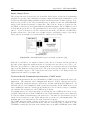
The frontal lobes are the part of the brain where the personality is generated and is located
at the front of the brain, see figure 3.1.
Figure 3.1: The structure of the brain[17]
Frontotemporal dementia, also called Pick’s disease, is a brain disease, which especially
affects the frontal lobe and the temporal lobes. Frontotemporal dementia is the fourth
most frequent cause of dementia and patients suffering from this make up for 5-10% of the
dementias.[39][26][15]
Frontotemporal dementia occurs in the age of 35-70 and affects men and women equally[39][15].
Patients suffering from frontotemporal dementia often get a personality disturbance, start
wandering, may behave different and often, their ability to speak is affected. Some patients
become unable to say anything but a word or two, while others speak fluently but without
content. The change in personality can differ from person to person. Some people exhibit
apathy, while others become overactive[13]. In this project the focus will be on the last
group. These patients tend to hide their jewelery and other personal belongings, because
they want to be sure of not loosing it, but they forget that they did it. Some of the patients
do not like to let the staff bath them or help them to the toilet, so the staff let the patients
do it on their own [1].
The patients can also suffer from depression or present minor mood alterations. The memory
and the sense of direction are either influenced late in the process or not at all. Frontotemporal dementia starts slowly and the symptoms are gradually deteriorating until death occurs.
The average course of the syndrome spans around ten years, from the first symptoms to
3.2. Frontotemporal Dementia
9
death[13]. There has not been found a cure for frontotemporal dementia, but the patients
receive medicine to be calmed down.[15] Music therapy is an alternative to medicine, and it
is also used to calm down the patients [1].
Chapter
4
Music Therapy
4.1
Music Therapy in General
Music therapy is a method that uses musical interaction in order to help people with mental
or physical illness and to enhance quality of life.[14]
In certain cases music therapy can support some treatments by e.g. strengthening the
immune system by dissipating tension. It has been proved that the therapy has positive
effects on quality of life and also on patients in connection with operations, chemotherapy
and in reducing anxiety [33]. Music therapists are working with a variety of physical and
psychological symptoms. The therapists design the music sessions for individuals based on
need and music preferences.[41] In a music therapy session music can be used both actively
and passively. Active music therapy includes instruments and passive music therapy includes
singing and listening to music. Mostly, the therapist starts singing and sometimes the patient
starts singing along. It is not necessary that the patients can play an instruments or sing,
the important thing is that the patients feel that they are seen and heard during the session.
Music therapy can take place in group sessions or individual sessions.[30]
Music therapy is e.g. used with patients suffering from frontotemporal dementia to calm
them down. This will be further described in the following section.
4.2
Music Therapy and Dementia
The patient group suffering from frontotemporal dementia is often highly medicated to calm
them down. This high intake of medicine may result in patients falling, causing broken bones
and teeth. These are some of the main reasons why it is important to find a way to calm
the patients down without pacifying them, and without medication. Otherwise there can
be consequences if the medicine is not dosed very precisely. It would be positive to keep
the patients calm in a natural way, without medicine. This is where music therapy can be
useful. During a music therapy session the calming element in the voice is used instead of
medicine.[1][9] The songs are being chosen together with the relatives, but even unknown
songs might be effective, as the voice itself has a calming effect when the therapist sings.[1]
In a music therapy session the therapist sings what is going to happen instead of saying
it because the patient finds it easier to relate to a song. A session always begins with the a
song and ends with the same song. During a session, the therapist sings for the patient for
11
12
Chapter 4. Music Therapy
about 20-30 minutes.
Patients with dementia recognise the songs and the music therapist which sooths the patient.
The patient sometimes starts the session with restless wandering but often will the patient
sit down next to the therapist and sometimes even fall asleep. It is different from patient to
patient how many sessions of music therapy they need to get the soothing effect. Patients
with severe dementia receive sessions on a daily basis, but for patients suffering from a milder
form of dementia one session a week will be sufficient.[1]
To show the effects of music therapy, music therapist Hanne Mette Ochsner Ridder, music therapist with area of specialisation in dementia, has measured the heart rate of six
patients [1]. In the study, heart rate was measured at the same time every day one week
prior to receiving music therapy. Afterwards, the patient received music therapy for four
weeks, five times a week. During the sessions the heart rate was measured. An entire week
after the last session, the heart rate was measured again showing a significant fall in heart
rate, compared to the heart rate measured before the music therapy session. This test has
only been performed in a single case design on six patients and it is not enough to meet the
requirements for entering the Cochrane database, because the test has to be scientifically
proved. 38 clinical empirical studies made from 1986 to 1998, show that music therapy can
be structured effectively to e.g. decrease behavioral problems[9].
Even though music therapy seems useful on patients suffering from sorrow, depression,
schizophren, dementia or some other disorder, it is not wide spread in Denmark. In other
countries, music therapy are wide spread but in Denmark only about 12 students are accepted at the education in music therapy every year since 1982, 80 % of them graduate.[7]
Music therapy sessions are rather expensive, because of the low numbers of therapists in
Denmark. Since the sessions are so expensive, the relatives of the patient or the patient
itself, often would not pay the price for something which is not scientifically proved.
Chapter
5
Problem Statement
5.1
Synthesis of Problem Analysis
The prevalence and incidence of dementia were estimated to 78.900 and 13.300 respectively
in Denmark in 2004[3]. Frontotemporal dementia is the fourth most frequent cause of dementia and patients suffering from this make up for 5-10% of the dementias [26]. Patients
suffering from frontotemporal dementia often get a personality disturbance. Some patients
tend to get overactive, which means they wander. Wandering is per se not unhealthy for
the patients, but if the patients wander at night instead of sleeping, it becomes a problem.
Wandering can be a sign of the patient’s state of mind. Perhaps the patients are aggressive
and restless, and therefore wander instead of sleeping.[1].
To calm down the patients, medicine is administered, which can cause them to fall. To
avoid medicating the patients, music therapy has been used as a calming method. The
music therapist often sings known songs to the patients, and structures the session, which
means that the music therapist sings a song in the beginning and the same song in the
end of a session. After a few sessions, the patients become familiar with the situation. Even
though the patients might not remember it, they can recognise the situation and the patients
become more relaxed for every session.[1].
Through the problem analysis, it has become possible to answer the initiating problem.
The experiment conducted by music therapist Hanne Mette Ochsner Ridder, shows that
music therapy has a calming effect on patients suffering from frontotemporal dementia.
A music therapy session is quite expensive and time demanding, and the impact on the
patients is not scientifically proved. Therefore, it is difficult to convince the relatives that
music therapy is beneficial for the patients. There is a need for quantitative research which
can prove that music therapy helps to calm the patients down, resulting in less wandering
at night.
This has lead to the following problem statement:
How is it possible to develop a system, which can measure the activity level
of patients, suffering from frontotemporal dementia who tend to wander?
13
14
Chapter 5. Problem Statement
Under the “problem solving” this statement will be attempted to be answered. Through
the problem analysis some general requirements regarding the system have been specified,
this will lead to the choice of a measurement method and sensor that will be used in this
project.
Part II
Problem Solving
15
Chapter
6
System Requirements
In the previous part, the initiating problem of the project has been analysed. This analysis
has made it possible to do an overall requirement specification. In the following, there will
be an analysis of the requirements, which will result in some more specific requirements.
These have been ordered into two groups:
• Functional requirements
• Other requirements
The functional requirements are functional demands to the system (as output, calculations
etc.), while other requirements impose constraints to the design of the system (e.g. placement, size etc.)
6.1
Functional Requirements
• The patients’ level of activity shall be registered.
• Because the patients can walk around during the night, the system must be able to
register in a 24 hour period of time.
• It is not expected that the staff have technical literacy, therefore, the system must be
easy to handle.
6.2
Other Requirements
The system:
• has to be placed out of immediate reach of the patients, since the patients tend to
remove unfamiliar objects.
• has to be low-cost since the patients tend to hide or destroy unknown objects.
• has to be low weight, so it does not annoy the patient.
• has be robust since the patients tend to hide or destroy unknown objects.
17
18
Chapter 6. System Requirements
• has to be safe to the patient, without any risk of electrical shock.
• has to be possible to construct the system within the period of the project.
The primary goal in this project is to develop a system that should be able to measure the
patients’ activity level in a 24 hour period. The developed system has to be small, low weight
and able to be placed where it does not attract attention from the patients.[1]
Chapter
7
Methods to Measure Level of
Activity
In order to determine the level of activity in patients suffering from dementia, different
methods have to be considered. A lot of physiological changes happen when e.g. change of
gait occurs or when ones mood changes. There are several methods available to measure
these changes, but especially with this group of patients, there are certain complications
connected to some of these methods. By analysing the possibilities and limitations of the
considered methods of measurement, it should be possible to decide which method would be
suitable for this purpose. The following methods will be discussed in this chapter:
• Pedometer
• Goniometer
• Force Sensing Resistor
• Global Positioning System
• Electromyography
• Accelerometer
7.1
Pedometer
A pedometer is a small device that registers and counts number of steps. This, however,
can be difficult to place on the patient without the patient either noticing, removing and
in worse case hiding or breaking it. Furthermore, the pedometer is not the most exact way
to measure the activity level, since it counts the total number of steps in a given period
of time. It is not possible to determine when each step is performed. This data does not
contain enough information about the gait to describe the effects of music therapy. Walking
itself is not harmful to the patient and therefore knowing only the total number of steps is
not useful in this case [1]. To increase accuracy the pedometer has to be placed at the hip,
which is in the immediate range of reach of the patient. As stated in chapter 3, patients
suffering from frontotemporal dementia sometimes wander around at night [1]. This would
be difficult to register with a pedometer since it is not possible to register when a specific
step is performed.
19
20
Chapter 7. Methods to Measure Level of Activity
7.2
Goniometer
A goniometer is an instrument for measuring the angle over a joint e.g. elbow, knee, hip
or ankle. By placing a goniometer at the knee, ankle or hip joint it is possible to register
each time a stride is performed. Thereby, it is possible to register whether the subject is
walking or not. Furthermore, it would be possible to analyse the output, using e.g. Matlab
to determine how fast the patient walks, but not the distance covered. There are some
limitations when using the goniometer on this group of patients. As described in chapter
3, some of the patients will remove the goniometer if they find it annoying. Therefore, it
will not be possible to use a goniometer placed at the hip and possibly not at the knee. By
placing it at the ankle joint, less of the patients would be able to reach the goniometer and
remove it.
The goniometers available for this project are the SG150 and SG110/A from Biometric Ltd.
The weight of these models are 19 g and 20 g respectively and can be mounted using double
sided tape. The lifetime of the sensors is approximately 600,000 cycles. The goniometers all
functions the same way, only differentiating in size to fit different joints. SG150 is specialised
for the hip and the knee. The SG110/A is used on the ankle where the measured output is
dorsiflexion/plantarflexion and inversion/eversion movements. The location and size of the
SG110/A makes it possible to measure the activity level of the patients. The price of about
5600 DKR,for the SG110/A is, however, a drawback. [31] [2]
7.3
Force Sensing Resistor
Force Sensing Resistors (FSR) consists of a polymer thick film that converts an increase in
applied force to a decrease in resistance. The force sensor available is the FlexiForce A201100 from TexScan. The diameter and thickness of the sensing area of the sensor are 0.95 cm
and 0.21 mm respectively. The FlexiForce A201-100has a lifetime of 10,000,000 cycles. The
length of the sensors are 203mm, 152mm, 102mm and 51mm. The cost of the sensors are
$99 for eight sensors. [45]
By placing the force sensor under the foot of the patient it will be possible to register when
the patient place weight on that foot i.e. when the patient is walking. The benefits of the
force sensor when used on the patient group are:
• The sensor is small and can be adjusted to fit the patient.
• Easy to place under the foot using double sided tape or inside a shoe.
• The sensor is inexpensive considering its lifetime.
• The sensor is placed under a foot making it difficult for the patients reaching and
removing it.
The output of the sensor can be visualised as a graph where the resistance is shown over
time, with a peak each time pressure is applied to the sensor. By analysing the graph it will
be possible to calculate the time between each step, i.e. if a patient is moving faster and
amplitude of each peak corresponding to how aggressively the patient is walking. It is not
possible to calculate the distance traveled.
7.4. Global Positioning System
7.4
21
Global Positioning System
Global Positioning System (GPS) can be used to determine the position of the patient. The
position is determined by the use of GPS-satellites circling in the atmosphere of the earth.
The accuracy can be affected by different spherical disturbances, in general the precision is
approximately ± 15 m varying from model to model. By knowing the position of the patient
at all time it is possible to calculate the average velocity of the walk. The GPS has the
advantage that it does not use a specific biomedical signal and can be placed anywhere it is
convenient e.g. under a wrist watch or in a shoe. Furthermore, it will be possible to locate the
patient if he/she leaves the nursing home, using the GPS. A project from Architecture and
Design at Aalborg University has examined the possibilities in using GPS for determining
the activity level of people walking in parks in the city. The project had some problem in
determining the indoor wandering due to disturbances’ from walls and concrete. [1] [16]
Furthermore, some other problem may occur: namely, if the patient is wandering around in
a circle and the GPS is unable to register that the patient is moving, the wandering will not
be registered. These deviations will result on inaccurate calculations and thereby produce
unreliable data. [10]
7.5
Electromyography
Electromyography (EMG) is a measure of muscle action potentials. The method can be
performed both invasive and non-invasive. The invasive method uses needle electrodes that
are inserted directly into the muscle. The output signal has an amplitude off 0.1 - 5 mV [27].
This procedure may be connected with pain and the inserting point may become inflamed
if used over a longer period. The non-invasive technique, called surface electromyography
(sEMG), uses skin surface electrodes to measure action potentials in the muscle. The surface
electrode can be placed on specific leg muscles used while walking e.g. Gastrocnemius medialis, Tibialis anterior or Rectus femoris. By measuring the action potentials it is possible
to register each time a step is taken. There is, however, some drawbacks when using surface
electrodes: the amplitude of the measured signals is smaller than when measured directly
in the muscle. This means that the need for signal amplification is greater than in invasive
measurements. In addition artifacts from e.g. skin impedance, other action potentials and
electrical interference have to be removed before analysing the signal. [27]
7.6
Accelerometer
An accelerometer is an electromechanical device that measures acceleration forces. There
are two types of these forces: static, like the constant force of gravity, and dynamic, caused
by moving or vibrating an object. By sensing the amount of dynamic acceleration, it is
possible to analyse the way the device is moving. [8].
Acceleration is defined as the time rate of change of velocity. In other words, acceleration is a measure of how fast the speed of an object is changing. Acceleration is measured
in m/s2 . Sometimes acceleration is denoted with a g, which is a unit of acceleration equal
to Earth’s gravity at sea level [18].
In analysing human gait, measurement of dynamic acceleration could be applied. By placing
22
Chapter 7. Methods to Measure Level of Activity
an accelerometer on a subject it would be possible to collect a voltage signal corresponding
to the acceleration of the subject. By applying computer algorithms using e.g. Matlab, this
signal could be analysed. It would be possible to identify the heel strikes of the subject and
thereby count the number of steps performed. By placing the accelerometer on the leg of the
subject, e.g. on the ankle, it would be possible to register any tremors of the leg and possibly
identify and differentiate between various types of gait and gait events. Furthermore, the
accelerometers property of measuring static acceleration could be used to measure tilt with
respect to gravity. Accelerometers are available as relatively small (0.5 mm times 0.5 mm),
low-cost(200 DKR) and durable integrated circuits. [11]
7.7
Selecting a Method of Measurement
In the previous section there has been a description of different types of sensors which are
able to measure the level of activity. When selecting the sensor to use in this project, several
parameters(stated in chapter 6) have to be considered. These parameters are:
• Placement
• Cost
• Size
• Analogue signal processing
• Possibility for gait analysis
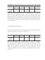
These parameters together with the different sensors, have been placed in table 7.1. The
sensors have been given a score from one to three for each parameter in order to determine
how well the specific sensor would do in this project.
• 1 was given if the sensor would perform with zero or few complications or disadvantages
in relation to the parameter.
• 2 was given if the sensor would perform with some or moderate complications or
disadvantages in relation to the parameter.
• 3 was given if the sensor would perform with several or severe complications or disadvantages in relation to the parameter.
7.7. Selecting a Method of Measurement
Sensor
Pedometri
Goniometer
FSR
GPS
EMG
Accelerometer
Place
-ment
2
1
1
1
3
1
23
Costs
Size
1
3
1
2
1
1
2
2
1
1
2
1
Analogue
Signal Processing
1
2
2
1
3
2
Possibility for
Gait Analysis
3
1
2
3
2
1
Table 7.1: The table shows the results of the evaluation of the different methods.
From the considerations in table 7.1, it is concluded that the sensor, which will be used,
is the accelerometer. An accelerometer can be placed anywhere on the body surface (with
different output signals), it is inexpensive, small and does not need complicated analogue
signal processing.
In this project it is chosen to place the accelerometer on the ankle, because it is out of reach
of the patient. Also it is chosen to do the test with bare feet and on a hard surface.
Chapter
8
Specifications
8.1
Hardware Specifications
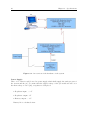
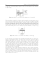
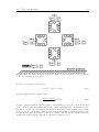
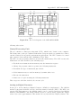
The purpose of this chapter is to set the specifications for the hardware of the system. Figure
8.1 shows an overview of the system, where the hardware part is specified.
Accelerometer and Evaluation board
The accelerometer used in this project is the ADXL311. The ADXL311 is capable of measuring both positive and negative accelerations to at least 2.0 g, see appendix C.1 for further
explanation. The accelerometer is mounted on an evaluation board, which has an adjustable
bandwidth provided by a 1. order low-pass filter, for further explanation see section 9.1.3.
The bandwidth is set to ≈ 20 Hz to minimise noise and to avoid aliasing.
• Evaluation board/accelerometer input from power supply: 3 V
• Accelerometer output range at Vdd = 3 V: 1,152 - 1,848 V
• Accelerometer current consumption: typical current consumption at 3 V is ≈ 400 µA
• Evaluation board bandwidth: 0 - 20 Hz
Micro Controller and Evaluation Board
The µC used in this project is MSP430f2274RHA. The µC is mounted on an evaluation
board named eZ430-RF2500.
• µC signal input range: 0 - Vcc .
• µC current consumption:
– Active Mode: 270 µA
– Standby Mode: 0.7 µA
– Off Mode (RAM Retention): 0.1 µA
• CC2500 2.4 GHz radio frequency transceiver
– CC2500 current consumption in transmit mode with 0dBm output power: 21.2
mA
25
26
Chapter 8. Specifications
Figure 8.1: An overview of the hardware of the system
Power Supply
Three 1.5 V batteries will be used as power supply, which shall supply the analogue part of
the system and the µC. To ensure that the supply voltage of the µC would not raise over
the max voltage of 3.6 V [22], a regulator is being used.
• Regulator input: > 3 V
• Regulator output: 3 V
• Battery output: > 3 V
Battery life is calculated from:
8.2. Software Specifications
T =
27
battery capacity in Ah
T otal current through the system
⇒
3600 · 10−3 Ah
≈ 159h
0.5 · 10−3 A + 750 · 10−6 A + 270 · 10−6 A + 21.2 · 10−3 A
From these specifications it is possible to design, implement and test every part of the
analogue system.
T =
8.2
Software Specifications
This section will provide the specifications of requirements of the software in the project. The
requirements have been divided into two groups: user requirements and other requirements.
The user requirements have been illustrated by use case diagrams.
8.2.1
User Requirements
These are requirements set by the user of the system. In this case the care taker or the music
therapist. In this section, there will be a description of the functional requirements and a
description of other requirements.
Functional Requirements:
It should be:
• calculate swing and stance phase.
• possible to detect strides taken by the patient and count these.
• able to perform self test on the system and indicate result to the user. Self test should
react to:
– low battery
– false signal from accelerometer
– false AP/ED setup
• visualise data.
Other Requirements
The other requirements are:
• The system should be able to work on the MSP430f2274RHA µC.
• Matlab should be used for the graphical user interface on the computer.
• The size of the program has to be as small as possible, occupying a maximum of 32
kB [22].
• The system should be able to read data from the accelerometer.
28
Chapter 8. Specifications
• The system should be able to save data on the ED.
Filter Specification
It is chosen to use a digital filter to remove noise.
The specifications of the digital filter is chosen in C.5:
• Cut-off frequency is set to 20 Hz.
• Stopband edge frequency is set to 35 Hz.
• The sampling frequency is 70 Hz.
8.2.2
Use Cases
In this section the functional requirements will be illustrated in use case diagrams. There
will be separate use case diagrams for the ED, the AP, and the Matlab program.
The use case diagrams will be followed by an explanation of the functions.
The diagrams consist of actors and functions performed by the system to the actors. The
actors interface with the given system. Thus, the actors are outside the system, but interacts
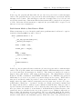
with the system. In the diagrams the actors will be notated as in figure 8.2.
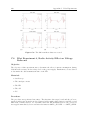
Figure 8.2: Notation of an actor in the use case diagrams.
The use cases will be notated by ovals, see figure 8.3. If a function is included in several use
cases, this will be notated by an arrow from the use case including the function, to the other
use case which is being included. This is illustrated in figure 8.3.
Figure 8.3: Use case diagrams notated by ovals. Use case 1 includes use case 2.
8.2.3
End Device
Receive Data
Receive data from the accelerometer.
Scenario:
1. Collect data from accelerometer.
8.2.3. End Device
29
Figure 8.4: The use case diagram for the ED
Exceptions:
The accelerometer is removed or damaged. The battery is empty.
Filter Data
Receives data from the accelerometer and filter the data.
Scenario:
1. Receive data from accelerometer(include: Receive data).
2. Filter data.
Exceptions:
The accelerometer is removed or damaged. The battery is empty.
Save Data to Flash Memory
Data received from the accelerometer will be saved in flash memory, and transmitted to AP
when all data have been collected.
Scenario:
1. Receive data(includes: Filter Data).
2. Save the data in flash memory.
Exceptions:
No data have been received from the accelerometer or the battery is empty.
All desired data have been received.
30
Chapter 8. Specifications
Transmit Data
Scenario I: Transmit collected data to the AP when all desired data have been received.
Scenario II: Transmit data live to the AP.
Scenario I:
1. All desired data have been received.
2. Connection to AP succeeds.
3. Transmit data from flash memory to AP.(includes: Save data to flash memory)
Exceptions:
No data have been received from the accelerometer or the battery is empty.
The AP is out of reach, not connected to the PC or have lost power after ED has been
activated.
Scenario II:
1. Connection to AP succeeds.
2. Transmit data to AP.
Exceptions:
Equal to the exceptions in scenario I.
8.2.4
Access Point
Figure 8.5: The use case diagram for AP
8.2.5. Matlab
31
Receive Data
Receives data from ED.
Scenario:
1. Find and recognise the ED.
2. Receive data from the ED.
Exceptions:
No signal from the ED. No data received by ED.
Transmit Data
Transmits data received from ED to Matlab.
Scenario:
1. Get data from ED. (Includes: Receive Data)
2. Transmit data to Matlab.
Exceptions:
The AP is not connected to the computer or there is no available data to transmit.
8.2.5
Matlab
Figure 8.6: The use case diagram for Matlab
32
Chapter 8. Specifications
Receive Data
Receive data from AP.
Scenario:
1. Find the AP.
2. Receive data from AP.
Exceptions:
Fails to connect to AP or no signal to receive.
Visualise Data
Display saved data or analysed data on a screen through a graphical user interface (GUI).
Scenario:
1. Read data.
2. Display data
Exceptions:
No data received/ no data stored.
Load Patient Data
Load information on the patient given by the user via the GUI.
Scenario:
1. Receive patient information.
2. Save data.
Exceptions:
No data given by the user.
Save data
A record is created where the patient information given from the user, the received data,
analysed data and the results from the comparison.
Scenario:
1. Create the record named after the patients civil registration number(include: receive
patient data).
2. Save the data received from AP in the record(include: receive data).
8.3. Accept Test of the Hardware
33
Exceptions:
No data to save.
Analyse data
The user chooses analysis to be carried out.
Scenario:
1. Create the record named after the patients civil registration number(include: receive
patient data).
2. Save the data received from AP in the record(include: receive data).
Exceptions:
No data to analyse.
8.3
Accept Test of the Hardware
In section 8.1, the hardware specifications are introduced. In this section it is explained how
these specifications will be tested.
8.3.1
Regulator
The regulator input should be over 3 V.
1. Measure the total voltage of the three batteries used.
The output of the regulator should be 3 V.
1. Apply different voltages to the regulator
2. Measure the output of the regulator
8.3.2
Evaluation Board/Accelerometer
Input on evaluation board/accelerometer should be 3 V.
1. Verify the output from the regulator is equal to 3 V.
Evaluation board/accelerometer Output: up to 3 V
1. Verify the input on evaluation board/accelerometer is 3 V.
2. The accelerometer can only give an output up to Vcc , hence the output will not exceed
3 V.
34
Chapter 8. Specifications
8.4
Accept Test Software
In section 8.2 a number of software specifications are introduced. In this section, it is
explained how these specifications will be tested.
8.4.1
Functional Requirements
The functional requirements will be tested as follows.
It should be possible to detect strides taken by the patient and count these.
1. Place system on person.
2. Walk x number of steps.
3. See how many strides the system has detected and counted.
It should be able to compare data regarding before, during and after a music
therapy session.
1. Record data in three different times.
2. Load data.
It should be able to perform self-test on the system and indicate result to the
user.
1. Start up system.
2. Perform self-test.
3. Observe result on LEDs.
It should be able to visualise potential errors.
1. Disconnect the accelerometer from the µC.
2. See alarm that indicates an error.
8.4.2
User Requirements
The user requirements are tested as follows.
The system should be able to work on the MSP430f2274RHA µC.
1. Start up the system on the MSP430f2274RHA.
2. Test the individual functions and the entire system. These tests will be further explained in section 10.2.
Matlab should be used for the graphical user interface on the computer.
1. Confirm all functions operates correctly.
8.4.2. User Requirements
35
The size of the program has to be as small as possible, with a maksimum of 32
kB.
1. Check up on the size of the program by creating a memory map in IAR Embedded
Workbench IDE.
2. Confirm that the size of the program is under 32 kB.
The system should be able to read data from an accelerometer.
1. Connect the accelerometer to the µC to check the connection between them.
2. Connect the accelerometer and µC to power supply.
3. Observe the µC has received data from the accelerometer.
The system should be able to save data on ED.
1. Configure the system to save to flash memory.
2. Input signal on ED.
3. Get saved data from ED.
Chapter
9
Design and Implementation
In this chapter the design and implementation of the modules in the hardware and the
software will be described. In the first section the hardware will be described and in the
following section the software.
9.1
Hardware Design
The analogue circuit consists of a power supply, an accelerometer and an evaluation board.
The different parts of the analogue circuit will be explained in the following sections.
9.1.1
Power Supply
The power supply supplies the evaluation board (including the accelerometer) and the µC.
The power supply consist of three batteries, a voltage regulator and a dual dip switch.
The batteries are regular AAA-batteries. The AAA-batteries are alkaline batteries with a
nominal voltage of 1.5 V giving a total voltage of 4.5 V. The rated capacity of a battery is
1200 mAh giving a total of 2600 mAh.
The voltage regulator is of type LE30CZ from ST Microelectronics. It has a typical output
voltage of 3 V. The voltage from the battery is regulated and then lead to a double dip
switch, which enables the user to turn on or off the power of the evaluation board, that
includes the accelerometer, and the µC individually. A diagram of the power supply can be
seen in figure 9.1
9.1.2
Accelerometer
The accelerometer that is used in this project is the AD XL311. The ADXL311 is a dualaxis acceleration measurement system on a single, monolithic integrated circuit. Dual-axis
means that the accelerometer is capable of measuring acceleration in two directions simultaneously. The two output signals are analogue voltages proportional to acceleration in the
two directions X and Y. At the typical input voltage, Vdd = 3V , the sensistivity at X and
Y is 174mV /g with a tolerance of ±15% and at all input voltages the output is nominally
Vdd /2 at zero g, see figure 9.2 [11]. The ADXL311 is capable of measuring both positive and
negative accelerations to at least ± 2 g. The accelerometer is capable of measuring static
acceleration forces such as gravity, allowing it to be used as a tilt sensor. The quiescent
supply current is typically 0.4 mA. [11]
37
38
Chapter 9. Design and Implementation
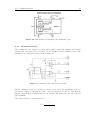
Figure 9.1: Diagram of the power supply. The 4.5 V of the batteries are regulated through
the 3 V regulator and distributed to the µC and the evaluations board (accelerometer) via
a double dip-switch.
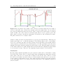
Figure 9.2: The figure shows the theoretical output response according to the orientation
of the accelerometer at rest. [11]
9.1.2. Accelerometer
39
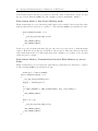
Figure 9.3: Pin configuration of the ADXL311. [11]
The pin configuration of the ADXL311 is shown in figure 9.3 and the pin function description
is given in table 9.1.
Pin No.
1
2,4,5
3
6
7
8
Mnemonic
ST
NC
COM
Yout
Xout
VDD
Description
Self Test
Do Not Connect
Common
Y Channel Output
X Channel Output
2.4 V to 5.25 V
Table 9.1: Pin function descriptions [11]
The self test pin controls the accelerometer’s self-test feature. When this pin is set to VDD
the resulting signal output is used to test if the accelerometer is functional. The typical
change in output is 0.290 g (corresponding to 50 mV). This pin can be left open circuit or
connected to common in normal use. In this application, the self test pin is grounded, see
section 9.1.3. [11]
The Function of the ADXL311
Accelerometers are constructed in many ways. Some use the piezoelectric effect, they contain
microscopic crystal structures that get stressed by accelerative forces, which causes a voltage
to be generated. Another method is to sense changes in capacitance. If two microstructures
are placed next to each other, they have a certain capacitance between them. If an accelerative force moves one of the structures, then the capacitance will change. The ADXL311
senses changes in capacitance. It consists of a variable differential air capacitor whose plates
are etched into a suspended polysilicon layer. The moving plate of the capacitor is formed
by a large number of "fingers" extending from a "beam", a proof mass supported by tethers
anchored to the substrate. Tethers provide the mechanical spring constant that forces the
proof mass to return to its original position when at rest or at constant velocity. The fixed
plates of the capacitor are formed by a number of matching pairs of fixed fingers positioned
40
Chapter 9. Design and Implementation
on either side of the moving fingers attached to the beam, and anchored to the substrate,
see figure 9.4 [8].
Figure 9.4: Model of a acceleration sensor during zero acceleration [8]
When responding to an applied acceleration or under gravity, the proof mass inertia causes it
to move along a predetermined axis, relative to the rest of the chip. As the fingers, extending
from the beam, move between the fixed fingers, capacitance change is being sensed and used
to measure the amplitude of the force that led to the displacement of the beam. In other
words: as soon as the chip experiences acceleration, the distance between the fixed plates
and the movable plates increases. At the same time the distance between the other fixed
plate and the movable plate decreases, resulting in capacitance imbalance, see figure 9.5. [8]
Figure 9.5: Model of a acceleration sensor during acceleration [8]
To sense the change in capacitance between the fixed and moving plates, two square wave
signals of equal amplitude, but 180◦ out of phase from each other, are applied to the fingers
forming the fixed plates of the capacitor. At rest, the space between each one of the fixed
plates and the moving plate is the same, and both signals are coupled to the movable plate
where they subtract from each other resulting in a waveform of zero amplitude. During
acceleration more than one of the two square wave signals get coupled into the moving plate,
and the resulting signal at the output of the movable plate is a square wave signal whose
amplitude is proportional to the magnitude of the acceleration, and whose phase is indicative
of the direction of the acceleration.[8]
The signal is then fed into a buffer amplifier and further into a phase-sensitive demodulator,
which acts as a full wave-rectifier. The output is a low frequency signal, whose amplitude and
polarity are proportional to acceleration and direction respectively. See the block diagram
of the accelerometer in figure 9.6. The two internal 32 kΩ resistors have a tolerance of ±
15% and can be used to set the band width of the accelerometer by adding capacitors. [11]
This is explained in section 9.1.3.
9.1.3. Evaluation Board
41
Figure 9.6: Functional block diagram of the ADXL311. [11]
9.1.3
Evaluation Board
The evaluation board consists of a dual single supply operational amplifier and various
resistors and capacitors. The accelerometer is also mounted on the evaluation board. The
diagram of the evaluation board is shown in figure 9.7.
Figure 9.7: Diagram of the evaluation board [44]
On the evaluation board, it is possible to increase or decrease the bandwidth of the accelerometer, simply by changing the value of the two capacitors Cx and Cy . This filtering
improves measurement resolution and prevent aliasing. The higher the value, the narrower
the bandwidth.
The equation for the corner frequency is:
Fc =
1
2π(32kΩ)C(x,y)
42
Chapter 9. Design and Implementation
In this project, it has been chosen to set the band width to 20 Hz C.5, thus Cx and Cy can
be calculated as:
Fc = 20Hz =
1
C
= 0.249µF
2π(32kΩ)C(x,y) (x,y)
[11]
Cx and Cy should be 0.249µF . The surface mounted capacitors with the nearest nominal
values is a 0.270µF capacitor and a 0.220µF capacitor. The 0.220µF capacitor is physically
smaller and would be easier to mount in the given slots on the evaluation board, therefore
this is chosen. This gives a corner frequency 22.6 Hz, which is satisfactory, see equation 9.1.
Fc =
1
≈ 22.6Hz
2π(32kΩ)220µF
(9.1)
The function of the three 47Ω resistors R1 , R2 and R3 are unknown, as is the function of the
220kΩ resistor, R4 , which is coupled between the ’Do Not Connect’-pin of the accelerometer
and ground.
The capacitors C1 and C2 are both 0.1µF capacitors and are applied to decouple the operational amplifier and the accelerometer from noise on the power supply.
The OP284 acts as a unity gain current buffer on the X- and the Y-signal after the low-pass
filtration. The OP284 is a single supply dual op-amp and has a current consumption of
1.35mA at Vdd = 3V .
The components of the evaluation board are placed on both sides of the board. To offer an
overview of the placement of the components, figure 9.8 has been created.
Figure 9.8: Component sketch of the evaluation board. The left half of the figure represents
the top view of the evalutaion board with the pins (1 through 4) placed to the right. In the
right half of the figure, the board has been flipped over, thus representing the bottom view
of the evaluation board, with the pins placed to the left. The two red lines represent the two
connections which intersects the evaluation board.[44]
9.2. Software Design
9.2
43
Software Design
According to the use cases in section 8.2, the system has been split up in different processes.
In the following section the different processes in the ED the AP and in Matlab will be
described. These process designs have been made based on the software requirement specification.
In the first subsection the process design on the ED will be described, the next subsection
deals with the AP and the third subsection is about the GUI.
9.2.1
End Device
The main objective of the ED is to receive data, filter the received data, save it to flash
memory and transmit it to the AP when sampling period is done. In the following an
overview of the other functions in the ED is given, see figure 9.9.
Initialise Radio
This function initialises the communication between both the µC and the CC2500 radio and
the switches.
Initialise Micro Controller
This function performs further initializations for the µC. These include: the DCO and MCLK
are set to run at 8 MHz, Timer A is set to trigger interrupts at 1/70 second intervals, see
appendix D for further explanation.
Initialise/join network
This function establish connection between ED and AP.
Link to Access Point
This function sends a link request to the AP. When the link request creates a successful link
between the ED and the AP, the ED becomes part of the network created by AP.
End Device Self Test
This function tests whether the ED receives data from the accelerometer and whether the
data is within acceptable limits. If this is not the case, the red LED will be turned on and
indicate an error. If the data is acceptable, the green LED will be turned on. If the µC is
not initialised correctly no LEDs will be turned on.
Read Acceleration
This function reads data from the accelerometer on port P2.0 and makes an A/D conversion
using a 10 bits successive-approximation-register ADC.
Filter Data
This function filters the data using an IIR filter, see section 9.3.
44
Chapter 9. Design and Implementation
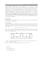
Figure 9.9: The processes in ED is illustrated in a flowchart. The arrows indicate the
direction of the data flow. The first interrupt from the push button connects the ED to
the AP. The second interrupt initiates the ED self test. The third interrupt starts the data
collection and send the data continuously to the PC. The fourth interrupt stops the flow of
data to the AP and saves data to flash instead. The fifth interrupt is used when 5 min of
data have been collected. After 5 min an interrupt makes the µC enter low power low where
it waits for the sixth interrupt. When the sixth interrupt have been received ED transmit
all collected data to the AP.
9.2.2. Access Point
45
Save Data in Flash Memory
This function saves data from ADC10 in flash memory on ED.
Transmit Data to Access Point
This function transmits all data saved in flash memory to AP. This function is performed
when all data has been received.
9.2.2
Access Point
The main objective of the AP is to receive data from the ED and transmit this data to
Matlab. In figure 9.10 the processes in the AP are illustrated. In the following an overview
of the modules in the AP is given, see figure 9.10.
Figure 9.10: The processes in the AP. The arrows indicates the direction of the data flow.
The flow will go through the sJoinSem[aphore] if a link request is sent from the ED. The
flow will go through the sPeerFrameSem[aphore] if the AP has received data from ED.
46
Chapter 9. Design and Implementation
Initialise Micro Controller
This function performs initialisations for the µC. These include: the DCO and MCLK are
set to run at 8 MHz, the Baud rate is set to 9600 and interrupts are enabled, see appendix
C.5.
Initialise board and drivers
This function initialises the communication between both the µP and the CC2500 radio and
the LEDs/switches.
Initialise Network
This function initialises the AP as the network hub.
Listen for a link
This function listens for a link request from the ED. When this link request is received a
successful link has been created.
sNumCurrentPeers++
This function increments the number of devices that the AP recognise as part of the network.
sJoinSem- This function decrements sJoinSem for another device to set.
Define input buffer
This function defines a message buffer in which to store the current frame. This is done every
time the sPeerFrameSem has been set or incremented, that is, every time the AP receives a
frame from the ED.
Process all waiting frames
This function loops through its input queues searching for frames until it has processed all
waiting frames.
Transmit data to PC
This function transmits frames to the PC. When doing so the green LED will be toggled
and the sPeerFrameSem will decrement.
9.2.3
Graphical User Interface in Matlab
In this subsection the design of the user graphical user interface(GUI) will be described. The
GUI has been implemented in Matlab.
The main objective in Matlab, is to receive data from the AP, analyse the data, save or
load data and visualise the data. Furthermore, it will be possible manual to compare data
9.2.3. Graphical User Interface in Matlab
47
collected before and after sessions of music therapy. In figure 9.11 an overview of the functions in Matlab is given.
Figure 9.11: The processes in Matlab. Matlab recieves data from the AP, and it is being
visualised right away. It is then possible to go to different modules. The user can choose to
save or load data, or to analyse the data. When the data have been saved it is also possible
to compare data from a previous data collection.
Receive Data
This module receives data from the AP.
Save/Load Data
This module allows the user to save or load data.
Analyse Data
This module identifies events of heel strike and toe off. These parameters are being used to
calculate the ratio of swing-stance phase. Furthermore, the cadence is being calculated.
Compare Data
This module allows the user to compare data received before and after sessions of music
therapy.
Visualise Data
This module visualises the results of the received data.
48
Chapter 9. Design and Implementation
9.3
Design and Implementation of Functions on End Device
In the following section the design of the most important functions in ED and AP will be
described. These sections are based on [21] and [22].
For each function there will be a short explanation.
Basic Configuration of Microcontroller
Configuration of the Analog-to-Digital Converter
When power supply is connected to the µC the basic configuration is automatically initialised
since these functions are placed before any interrupts are allowed. Therefore, no actions have
to be taken to setup the µC besides having an AP started.
A single channel from the accelerometer is A/D converted, the X-axis, to be used in the data
processing. The ADC is configured by the following code:
1)
2)
ADC10CTL0 = ADC10SHT_3 + ADC10ON + ADC10IE + ENC;
ADC10CTL1 = INCH_0;
Line 1: In the ADC10 control register 0, the ADC10SHT_3, ADC10ON, ADC10IE and
ENC are set. ADC10SHT_3, controls the sample-and-hold time, which in this case is 64
x ADC10CLKs. The commands ADC10ON and ADC10IE turn on the ADC10 and enable
interrupts from the ADC10 . The command ENC enables conversions. This must be set to
1 before any conversion can take place. In the ADC10 control register 0 the reference to the
ADC is selected with the command SREF_x. The reference is by default set to VR+ = VCC
and VR− = VSS and will therefore not be changed.
Line 2: In the ADC10 control register 1 INCH_0 is selected. While the ADC is running in
single channel mode, INCH_x selects the channel to be converted. In this case INCH_0 is
equal to channel A0 or pin3 on the evaluation board.
The command ADC10SC (start conversion) is placed in ADC10CTL0 in timer_A interrupt service routine, see section 9.3. To ensure that ADC10SC is placed in ADC10CTL0
without overwriting the previous setup, the bitwise OR assignment (|=) is used.
Configuration of Timers
1)
2)
3)
4)
TACCTL0 = CCIE;
TACCR0 = 57143;
TACTL = TASSEL_2;
TACTL |= MC_1;
Line 1: the capture/compare interrupts, CCIE, are enabled in timer A capture/compare
control register 0, TACCTL0.
Line 2: TACCR0 is the capture/compare register 0 in which the number 57143 is set, since
the desired sampling frequency is 70 Hz.
Line 3: the source of timer A defines timer A,. This property is set in TACTL, which is
the control register of timer A. The command TASSEL_2 chooses the clock source, which
in this case is the sub-main clock. The frequency of the sub-main clock is set to 4 MHz in
9.3. Design and Implementation of Functions on End Device
49
the configuration of the basic clock module in subsection 9.3 line 5. The reason for doing
this is to slow down the process, that counts to TACCRO, in order to obtain a more precise
sampling frequency.
Line 4: the timer A is set in up mode. Thus the timer A starts counting up to TACCR0(i.e.
57143) with a frequency of 4 MHz. This produces a frequency of 70 Hz, which is used as the
sampling frequency in the ADC. Timer B is not used in this project. [21] [22]
Configuration of the Basic Clock Module
To control the performance of the modules in the µC the basic clock module has to be
configured.
1)
2)
3)
4)
5)
BCSCTL1 = CALBC1_8MHZ;
DCOCTL = CALDCO_8MHZ;
BCSCTL2 |= SELM_1;
BCSCTL2 &= ~SELS;
BCSCTL2 |= DIVS_1;
Line 1: the basic clock system control 1(BCSCTL1) is set to run with 8 MHz.
Line 2: the internal digitally controlled oscillator control register(DCOCTL) is set to run
with 8 MHz.
Line 3: the main clock is selected as DCOCLK at 8 MHz. The usage of a bitwise OR
ensures the register to get the value 1.
Line 4: the sub-main clock source is selected to be DCOCLK. The bitwise AND ensures
the main clock to remain as DCOCLK.
Line 5: the sub-main clock is divided by two, to produce a frequency of 4 MHz. This is
done to set TACCR0 as high as possible to obtain a more precise frequency.
Configuration of I/O Ports
On the µC there are four available digital I/O ports, each having eight I/O pins. To control
these ports, each of them must be configured. Unused pins are configured as output pins to
prevent a floating input and reduce power consumption.
1)
2)
3)
4)
5)
6)
7)
8)
9)
10)
11)
P1DIR = ~BIT2;
P1REN |= BIT2;
P1OUT = BIT2;
P1IE |= BIT2;
P1IES |= BIT2;
P1IFG &= ~BIT2;
P2DIR = ~(BIT0 + BIT6 + BIT7);
P2REN |= BIT0;
P2OUT = ~BIT0;
P3DIR = 0xFF;
P3OUT = 0x00;
50
Chapter 9. Design and Implementation
12) P4DIR = 0xFF;
13) P4OUT = 0x00;
Line 1: sets P1.2 (General-purpose digital I/O pin) as input. This corresponds to the push
button. The rest is set as output. P1.0 and P1.1 are equal to the LEDs.
Line 2: Enables pullup/pulldown resistor on P1.2.
Line 3: pulls up the pin at P1.2, which will ensure that the signal at the port to the push
button always is stabil high.
Line 4: enables interrupts at P1.2.
Line 5: sets the P1IFG2 flag with a high-to-low transition. Thus, there will be an interrupt
on the falling edge.
Line 6: clears the interrupt flag register(IFG) for a new interrupt. This is done after each
push button interrupt, see subsection 9.3.
Line 7: sets P2.0, P2.6 and P2.7 as input. P2.0 corresponds to pin 3 on the eZ430-RF2500T
target board. P2.6 and P2.7 are used by the CC2500. All other ports are set as output.
Line 8: enables pullup/pulldown resistor on P2.0.
Line 9: pulls down the pin at P2.0, which will ensure, that there is no signal at pin P2.0
Line 10: sets all P3 pins as output since none of these are used.
Line 11: sets the output low in the output register, thus nothing can be measured at the
pins.
Line 12: sets all P4 pins as output since none of these are used.
Line 13: sets the output low on the output register.
Configuration of Flash Memory
The flash module of the µC contains 32000 bytes of memory. In this memory both code
and data have to be stored. Therefore, it is important to control that the data is not stored
in memory adresses where code is located. If data from the A/D conversions overwrites
memory where code is located, the results may be a reset of the µC, loosing all previous data,
unpredictable flash writing, making it impossible to read flash memory without errors, or the
µC can even be destroyed so that it can not be reprogrammed. When using IAR Embedded
Workbench IDE it is possible to create a memory map of the device being programmed. This
feature allows the programmer to get a clear overview of where in the flash memory, data can
be saved without any risk of overwriting code. This tool showed, that it was possible to save
data in the range from 0xAA10 (43536) to 0xFC18 (64536). In this range it is possible to
save 21000 8-bit conversions as hexadecimals. When sampling at 70 Hz, it makes it possible
to save up to 300 seconds of data in the flash memory. To save data in the flash memory
the flash module has to be initialised. This is performed by the following code:
1)
2)
3)
FCTL2 = FWKEY + FSSEL_2 + FN3 + FN1;
Flash_ptr = (char *)0xAA10;
FCTL3 = FWKEY;
All write and erase operations are controlled by the flash memory timing generator. The
operating frequency, fF T G of the generator must be in the range 257 kHz - 476 kHz. fF T G
is set in Flash Memory Control Register 2.
Line 1: initialises the Flash Memory Control Register 2, FCTL2. In this register a password,
FWKEY, for the register, is set. This must be set each time a register has to be altered.
9.3. Design and Implementation of Functions on End Device
51
In the register the flash controller clock source, FSSEL_2, is selected to SMCLK which is 4
MHz. Furthermore, the flash controller clock divider, FN3 and FN1, is set to 11. These two
setting give an operating frequency of:
4000000Hz
= 363.6kHz
11
(9.2)
which is within the desired range.
Line 2: defines the variable Flash_ptr to (char *)0xAA10. The data type char defines the
size of the data to be save each time a sample is saved in flash. A char contains 8 bits, which
is equal to the output of the ADC after compressing the result, see section 9.3. 0xAA10 and
the pointer * points to the address where the first sample is written.
Line 3: initialises the Flash Memory Control Register 3, FCTL3. By setting FWKEY, the
rest of the register is set to 0. This includes LOCK which, when it is unlocked, makes it
possible to write to flash.
Push button Mode 1, Join Network
The variable pushbuttonmode is defined as a char with the value zero during the initialization.
After the basic configuration of the µC, the program enters low power mode 1, LPM1, in
the following code:
while (pushbuttonmode != 1)
{
__bis_SR_register(LPM1_bits);
}
While the ED is waiting for new interrupt from the push button, it is in LPM1 to minimise
the consumption of current. The operation mode LPM1 is chosen, since the SMCLK is still
active. When an interrupt from the push button is received, pushbuttonmode increments
and the program leaves the while loop. Afterwards, the timer A is initialised and ED keeps
on trying to join the network, which is created by the AP. By the following while loop the
network is attempted to joined:
while (SMPL_NO_JOIN == SMPL_Init((uint8_t (*)(linkID_t))0))
{
__bis_SR_register(LPM1_bits);
}
After the network has been joined, the ED keeps trying to link to the AP with the following
while loop:
while (SMPL_SUCCESS != SMPL_Link(&linkID1))
{
__bis_SR_register(LPM1_bits);
}
52
Chapter 9. Design and Implementation
Each time the ED sends a frame to the AP, a linkID is placed in the beginning of the frame.
A frame is ten samples, which is also called the payload. This linkID, is send to make the
AP recognise whether the frame is a join request or a frame containing data from an already
known ED. A linkID equal to zero is interpreted as a join request and a linkID larger than
zero is interpreted as data frame reception, see section 9.4 for further description.
After the network is joined by the ED and the link to the AP is created, the program enters
the following while loop:
while (pushbuttonmode == 1)
{
__bis_SR_register(LPM1_bits);
}
As long as pushbuttonmode is equal to 1 the µC is in low power mode 1. The program will
wait in this loop until another interrupt from the push button is received.
Push button Mode 2, End Device Self-Test
When an interrupt is received from the push button, pushbuttonmode will now be equal to
2. The purpose of this mode, is to verify that the signal from the accelerometer is operating
as intended. This will be done by performing a self test. While testing, the ED must be
placed on a horizontal plane surface. In figure 9.12 the self-test is illustrated in a flowchart.
Figure 9.12: Flowchart for ED self test. The self test is only activated when the system is
in pushbuttonmode_2. If this is the case, A0 will be defined. Next it will be decided whether
A0 is above or below the expected limits. If the test is positive the green LED will be on, if
the test is negative the red LED will be on.
The function will test whether the battery, µC and accelerometer are connected and initialised correctly. The test is performed continuously while pushbuttonmode is equal to 2 in
the following code:
while (pushbuttonmode == 2)
9.3. Design and Implementation of Functions on End Device
53
{
A0 = msg[counter];
if ((A0 < 127) && (A0 > 122))
{
if (BSP_LED1_IS_ON())
{
BSP_TOGGLE_LED1();
}
BSP_TOGGLE_LED2();
}
else
{
if (BSP_LED2_IS_ON())
{
BSP_TOGGLE_LED2();
}
BSP_TOGGLE_LED1();
}
}
After entering the while loop the result from the A/D conversion is copied into the variable
A0. The if loop decides whether A0 is within expected limits. If A0 is within expected
limits, the red LED will turn off and the green LED will turn on to indicate a successful
test. A successful test is if the accelerometer is placed plane, and the same time is held
still. If this is not the case, the green LED will turn off and the red will be turned on. The
values which set the limits are 122 and 127. 122 and 127 are the same as 488 and 508 after
being bit shifted two to the right after the A/D conversion. With a power supply (voltage
reference to the ADC) of 3V, these values are equal to 1.43 V and 1.48 V, since the system
is not plane because of bolts to the accelerometer. If the system had been plane, the values
would be equal to 1.5 V. This test will thereby indicate if the accelerometer is connected
and functions correctly. The power supply is indirectly tested. If the power supply is lower
than 3V, the result from the ADC will not be within the stated range, since the ADC uses
the supply voltage as reference.
Push button Mode 3, Continual Transmit Data to Access Point
When an interrupt is received from the push button, pushbuttonmode will now be equal to
3 and enter the following while loop:
while (pushbuttonmode == 3)
{
__bis_SR_register(LPM1_bits);
if (SMPL_SUCCESS == SMPL_Send(linkID1, msg, sizeof(msg)))
{
BSP_TOGGLE_LED2();
}
54
Chapter 9. Design and Implementation
}
In the loop the program will first make the µC enter low power mode 1 with interrupts
enabled. The program will leave low power mode when an interrupt is set from the ADC10
interrupt service routine. This will happen each time 10 samples have been collected and
saved in the variable msg. This means that the if statement will be completed at a frequency
of 7 Hz. Each time the if statement is completed the green LED will be toggled, as an
indicator of successive transmission.
Push button Mode 4, Save Data to Flash
When an interrupt is received from the push button, pushbuttonmode will now be equal to
4 and the following while loop will be entered:
while (pushbuttonmode == 4)
{
__bis_SR_register(LPM1_bits);
__disable_interrupt();
FCTL1 = FWKEY + WRT;
*Flash_ptr++ = msg[0];
b++;
FCTL1 = FWKEY;
__enable_interrupt();
if ( b == 2100)
{
pushbuttonmode++;
}
}
In the loop, the program will start to make the µC enter low power mode 1 with interrupts
enabled. The loop will continue after an interrupt from the ADC10 interrupt service routine
is received and then, all interrupts are disabled. This ensures no unexpected events to
happen, that could interfere with saving in flash memory. The Flash Memory Control
Register 1, FCTL1, is initialised, and FWKEY and WRT are set. FWKEY is the password
which must be set before it is possible to perform changes in the register. WRT enables
write mode and thereby makes it possible to write in the flash memory. *Flash_ptr++ =
msg[0], writes the sample which is temporarily stored in array, msg, on place 0 to place
in flash where *Flash_ptr + 1 points to. In this case *Flash_ptr points to 0xAA10 and
the sample will therefore be written on place 0xAA11 in flash memory. This procedure is
repeated 10 times (not shown in the code) to write the entire array, msg, to the flash. After
these procedures, the variable b is incremented. In Flash Memory Control Register 1 the
password is now set and thereby the rest of the register is reset. Making it impossible to
write to flash. All interrupts are now enabled. The loop ends with asking if the variable
b has been incremented to the value 2100. When b reaches 2100, 21000 samples have been
written to flash which is the maximum capacity. When this event occurs, pushbuttonmode
9.3. Design and Implementation of Functions on End Device
55
is incremented and it will not be possible to enter the ’write to flash mode’ again. If b has
not yet reached 2100 the while loop will continue to run for maximum 5 minutes.
Push button Mode 5, Low Power Waiting mode
When an interrupt is received from the push button or the variable b has reached the value
2100, pushbuttonmode will now be equal to 5. The following while loop will therefore run:
while(pushbuttonmode == 5)
{
__bis_SR_register(LPM1_bits);
BSP_TOGGLE_LED1();
BSP_TOGGLE_LED2();
}
In the loop, the program will make the µC enter the low power mode 1 with interrupts
enabled. Both the green and the red LED are then toggled. This state indicates that the
entire flash memory has been filled with data from 5 minutes of recording or the user has
ended the prior recording.
Push button Mode 6, Transmit Data Saved in Flash Memory to Access
Point
When an interrupt is received from the push button, pushbuttonmode will now be equal to
6. The following while loop will therefore run:
Flash_ptr = (char *)0xAA10;
while (pushbuttonmode == 6)
{
__bis_SR_register(LPM1_bits);
msg[0] = (*Flash_ptr++);
b--;
if (SMPL_SUCCESS == SMPL_Send(linkID1, msg, sizeof(msg)))
{
BSP_TOGGLE_LED2();
}
while (b == 0)
{
__bis_SR_register(LPM1_bits);
BSP_TOGGLE_LED1();
BSP_TOGGLE_LED2();
}
}
56
Chapter 9. Design and Implementation
Before entering the while loop, the variable *Flash_ptr is set to point at the address
0xAA10, which is the same address as when beginning to write to flash memory. msg[0]
will at this point contain the values from the A/D conversion just performed. msg[0] =
(*Flash_ptr++); will overwrite msg[0] with the value from the initial flash address + 1,
which is 0xAA11. This procedure is repeated 10 times (not shown in the code), copying 10
samples into the array of msg. When the 10 samples are copied, the value b is decremented
and msg is transmitted to the AP the same way as in pushbuttonmode 3, see section 9.3.
When b reaches zero the program will enter the while loop where the µC enters low power
mode 1 and flashes both LEDs. The program will be in this state until power is reset and
the µC will execute the main function from the top. By letting b count down from where it
is set in pushbuttonmode = 5, section 9.3, no data will be read from the flash memory where
no data have been written to.
Digital Filter
It is chosen to use a digital filter to remove noise that may occur after the anti-aliasing filter
and to further specify the signal.
Filter Design
As stated in appendix C.5 a digital low pass filter is chosen. An IIR filter is chosen for this
application since it has a shorter execution time and since the order of the filter becomes
smaller than when using a FIR filter. The equation of the filter that is being implemented
is as follows:
y(n) = b0 x[n] + b1 x[n − 1] − a1 y[n − 1]
Where y(n) is the output, y(n-1) is the previous output, b0 , b1 and a1 are the filter coefficients,
x(n) is the input and x(n-1) the previous input. The flow of the signal in the first-order IIR
filter can be seen in figure 9.13
Figure 9.13: Signal flow graph of the first-order IIR filter.
The code is being implemented in ED and since the µC has only 32 kB memory, the code
has to be as compact as possible.
The filter coefficients were found by using the functions showed below:
Fs = 70;
n = 1;
Wn = 0.5714;
[c,a] = butter(n,Wn)
c = 0.5563 0.5563
9.3. Design and Implementation of Functions on End Device
57
a = 1.0000 0.1126
where n is the order of the filter. Wn is the "3 dB frequency" in rad, which are calculated
from 20/(F s/2). A and c are the filter coefficients which are used to design the filter in C.
Figure 9.14: The figure shows a linear phase response which means that all frequencies
experience the same time delay when passing through the filter.
After the coefficients were found, the phase response were checked out, see figure 9.14 and
so were the poles and zeros in the z-plane, see figure 9.15.
Figure 9.15: The pole(the cross) and zero(the dot) in the z-plane which shows that the
filter is stable since the pole is in the left half plane and lay inside the unit circle.
Implementation
Below the filter code can be seen. The flow diagram 9.16 shows what the code does step by
step.
#define FILTER_LENGTH 3
float x[FILTER_LENGTH]
float y[FILTER_LENGTH]
float a[FILTER_LENGTH]
float c[FILTER_LENGTH]
int n;
=
=
=
=
{0,0,0};
{0,0,0};
{1, 0.1126};
{0.5563, 0.5563};
58
Chapter 9. Design and Implementation
x[2] = temp[counter];
y[2] = c[0]*x[2]+c[1]*x[1]-a[1]*y[1];
for (n=0; n<=1; n++)
{
x[n] = x[n+1];
y[n] = y[n+1];
}
x[2] = temp[counter];
tmp[counter] = (signed char) y[2];
Figure 9.16: The flow diagram shows the code step by step from when the input is retrieved
until the filter is done processing it. First X and Y, where X is the input and Y is the output,
are set to an array of three zeros so that the filter equation has some previous values for both
input and output in the beginning. Afterwards, the filter coefficients, a and c, are stated.
x[2] = temp[counter]; gets a value, which is sent through the filter equation. The value y[2]
is first put in an array on the second place to be used with the next input, and then put in
temp[counter] for sending. The x values are likewise put in an array on the second place. In
the filter equation the previous two values for both x and y are being used so every time a
new value is being put into the array, the previous is being pushed left one place.
ADC10 Interrupt Service Routine
The following function is called each time an interrupt from ADC10 is received:
#pragma vector=ADC10_VECTOR
__interrupt void ADC10_ISR(void)
{
temp[counter] = (unsigned char)(ADC10MEM>>2);
tmp[counter] = (signed char) y[2];
counter++;
if (counter == 10)
{
for (counter = 0 ; counter < 10 ; counter++)
{
msg[counter] = tmp[counter];
}
counter = 0;
__bic_SR_register_on_exit(LPM1_bits);
}
9.3. Design and Implementation of Functions on End Device
59
}
The interrupt flag, ADC10IFG, from the ADC10 is set when a conversion result is saved
in ADC10MEM. The interrupt flag will automatically be reset when entering the ADC10
interrupt service routine. The result from the A/D conversion is located in ADC10MEM.
The result is bit shifted two to the right (»2), this is done since the COM-port is unable to
receive 10 bits, and saved as an unsigned char in the array temp, to make values go from
0 to 255. The place in the array is initialised to place 0 and the counter incrementation
will make sure that the entire array is filled. Each value in the array temp is evaluated by
the filter, see section 9.3, and saved into a new array tmp. When the entire array is full
the variable counter will be equal to 10, and the if statement will be entered. In this loop
the entire array tmp is copied into the array msg place by place. When the 10th sample is
copied, counter is reset and the µC enters low power mode 1.
Port 1 Interrupt Service Routine
When there is an input on P1.2(i.e. the button has been pushed down) the port 1 interrupt
service routine will be called. The following code shows the procedure for the interrupt
service routine.
__interrupt void Port_1(void)
{
volatile long l;
pushbottonmode++;
for( l = 0x186A0; l > 0; l-- );
P1IFG &= ~BIT2;
__bic_SR_register_on_exit(LPM1_bits);
}
When the push button has been pushed, the pushbuttonmode will proceed to the next mode.
After this, a delay will ensure the pushbuttonmode only to be added by one, while the interrupt activates on a falling edge and therefore could register more than one input.
After the delay(250 ms.) the interrupt flag is cleared for a new interrupt to set.
Timer A Interrupt Service Routine
The timer A0 interrupt service routine is called every time the timer A control has counted
to TACCRO(57143), which corresponds to 70 Hz. The following code shows the timer A0
interrupt service routine procedure.
__interrupt void Timer_A (void)
{
ADC10CTL0 |= ADC10SC;
}
60
Chapter 9. Design and Implementation
This starts sample and conversion. Thus sample and conversion is done with a frequency of
70 Hz.
9.4
Design and Implementations of Functions on Access
Point
Basic Configuration of Microcontroller
The MCU_Init() function perform necessary initialisations for the AP.
The following code shows how the function is called and the basic clock and DCO (Digitally
Controlled Oscillator) are set to run at 8 MHz. This is done the same way as on the ED.
BCSCTL1 = CALBC1_8MHZ;
DCOCTL = CALDCO_8MHZ;
In the following code the USCI clock source is selected to be the sub main clock(SMCLK)
that runs with 8 MHz. After this, the USCI_A0 baud rate control register is set to 9600
Baud.
Then the USCI_A0 control register is set to run with sub main clock by setting UCSWRST.
Then interrupts are enabled on USCI_A0 RX.
UCA0CTL1 = UCSSEL_2;
UCA0BR0 = 0x41;
UCA0BR1 = 0x3;
UCA0MCTL = UCBRS_2;
UCA0CTL1 &= ~UCSWRST;
IE2 |= UCA0RXIE;
__enable_interrupt();
Initialise Network
After the µC and the radio on the AP have been initialised, the network is initialised by
calling the following function:
SMPL_Init(sCB);
BSP_TURN_ON_LED1();
The sCB parameter, semaphore callback, is a function pointer to a callback function which
is executed when a message has been received by the AP. The Red LED is toggled to
indicate the network have been correct initialised. The following code shows the sCB callback
function.
static uint8_t sCB(linkID_t lid)
{
9.4. Design and Implementations of Functions on Access Point
61
if (lid)
{
sPeerFrameSem++;
}
else
{
sJoinSem++;
}
return 0;
}
The callback function identifies the received packet from ED as either a join request, or a
packet from an ED that has already established connection to the network. If the received
packet is from an already known ED (lid 6= 0), the sPeerFrameSem[aphore] will be incremented. If the linkID received is equal to 0 it will be identified as a join request and the
sJoinSem[aphore] will be incremented. Thus, the ED sends a linkID of 0 until connection to
AP has been established. When ED has established connection to AP, the AP assigns an
incremental linkID to the ED.
sJoinSem
After the network has been initialised, the program enters a while(1) loop which runs an
infinite number of times. Thus, the network will only be initialised once. The following
if statement will be entered when the sJoinSem[aphore] has been incremented in the sCB
callback function and the number of EDs connected to the network is lower than the max
number(NUM_CONNECTIONS), which is defined in smpl_config.dat to be eight connections by default.
if (sJoinSem && (sNumCurrentPeers < NUM_CONNECTIONS))
{
BSP_TURN_OFF_LED1();
SMPL_LinkListen(&sLID[sNumCurrentPeers]);
sNumCurrentPeers++;
if (sJoinSem)
{
sJoinSem--;
}
}
After entering the loop, the SMPL_LinkListen function will be called. This function will
not return until a successful link has been created. When a successful link has been created
the sNumCurrentPeers will be incremented and the sJoinSem[aphore] will be decremented
and thereby be ready for a new ED connection.
sPeerFrameSem
The following if statement will be entered every time the sPeerFrameSem[aphore] is incremented in the sCB callback function. This will happen every time AP receives a frame from
ED.
62
Chapter 9. Design and Implementation
if (sPeerFrameSem)
{
uint8_t
msg[MAX_APP_PAYLOAD], len, i;
for (i=0; i<sNumCurrentPeers; ++i)
{
if (SMPL_Receive(sLID[i], msg, &len) == SMPL_SUCCESS)
{
while (!(IFG2&UCA0TXIFG));
UCA0TXBUF = msg[0];
BSP_TOGGLE_LED2();
sPeerFrameSem--;
}
}
}
After entering the loop, three variables are defined. Then there is a for loop which runs
a number of times equal to the number of EDs connected to the AP. This loop separately
receives data from the ED connected to the network. The way this is done, is by checking if
the linkID, message and length of message are received.
The statement UCA0TXIFG is set in the register IFG2 when the UCA0 transmit buffer is
empty. This means that the program will enter the while loop (!(IFG2&UCA0TXIFG)) and
wait here until the buffer is empty and the flag is removed. When the flag is removed, the
value from the array msg on place 0 is copied into the buffer. This procedure is repeated
10 times to copy the entire array into the buffer (not showed in the code). Once the entire
array have been copied, the sPeerFrameSem[aphore] is decremented.
9.5
Data Analysis
In the following section the analysis of the acceleration signal will be explained. Matlab
receives the filtered acceleration signal from the AP and the data analysis is then executed
in Matlab.
The objectives of the analysis are:
• to identify the points of heel-strike.
• to count the number of strides.
• to identify the points of toe-off.
• to calculate cadence.
• to calculate swing-stance ratios.
The acceleration signal and the different gait events and phases can be seen in figure 9.17.
9.5. Data Analysis
63
Figure 9.17: The figure shows the x-axis acceleration signal of a complete gait cycle (one
stride). The actual and detectable gait events, the calculated gait phases and the threshold
values that are used in the data analysis are marked
Identifying Heel-Strike and Counting Strides
In appendix C.5 the heel-strike has been identified in the acceleration signal. The heel-strike
is visually detectable as a bend in the curve, succeeded by a negative peak (see figure 9.17).
Using simple algorithms in Matlab, it is easier to detect the peak than the bend. Identifying
the heel-strike as the peak instead of the bend will only provide a marginal delay to the
detected heel-strike compared to the actual heel-strike (1-2 samples, that is 1/70 s to 1/35
s). This will not have an effect on the number of strides counted, but it will provide an
equally marginal decrease of the stance-phase and an increase of the swing-phase.
To identify the heel-strike, a threshold is set in Matlab. See "tresholdHS" in figure 9.17.
When the value of the acceleration signal is below the threshold, it is compared if each value
is lower than the successive value. If the successive value is higher than the current value,
the current value must be a peak and is interpreted as the heel-strike. When the lowest value
succeeding the threshold is found, one stride is registered by incremented the value stride,
the point of heel-strike is registered by assigning HS(stride) with a value corresponding to
the sample number. Finally 21 samples are jumped ahead and the loop is exited. The jump
of 21 samples is found from analysing the signal and deciding how many samples, which are
convenient, see figure 9.18.
Identifying Toe-Off
In appendix C.5 the toe-off has been identified in the acceleration signal. The toe-off is taking place between negative peaks followed by a positive peak, see figure 9.17. Identifying the
toe-off as the positive peak will provide a marginal delay to the detected toe-off compared
to the actual toe-off (1-2 samples, that is 1/70 s to 1/35 s). This delay will counterbalance
64
Chapter 9. Design and Implementation
Figure 9.18: The figure shows the data flow of the loop that identifies the heel-strikes.
The loop runs as long as the current sample number, i, is lower than the total number of
samples, a. It is examined if the value of the current sample, xout, is lower than a preset
threshold value, thresholdHS. If xout is higher than or equal to thresholdHS, the next
sample is examined by incrementing i. If xout is lower than thresholdHS, p is assigned the
value of i + 1. Now, it is examined if xout is lower than the value of the sample, q(1,p).
If xout is higher than or equal to q(1,p), the next sample is examined by incrementing i
up by one. If xout is lower than q(1,p), the value stride is added by one, the point of the
heel-strike is registered by assigning the value HS(stride) = with the value of i and 21 is
added to i to skip analysis of the oscillations following the heel strike.
the delay of the detected heel-strike, see section 9.5.
To identify the toe-off, a threshold is set in Matlab. See "‘thresholdTOFF"’ in figure 9.17.
The toe-off occurs in the time span between one particular heel-strike, HS(h), and the successive heel-strike, HS2(h). HS is already identified, and HS2 is found simply by assigning
it with the value corresponding to HS(h+1). Matlab is set to search for the toe-off between
HS(h)+21 and HS2(h)-21, thus narrowing the search field, see figure 9.17. When the value
of the acceleration signal is higher than the threshold value, it is compared if each current
value is higher than its successive value. If the successive value is higher than the current
value, the next value is examined. If the successive value is lower than the current value,
the current value must be a peak and is interpreted as the toe-off. When the highest value
succeeding the threshold is found, the point of toe-off is registered by assigning TOFF(h)
with a value corresponding to the sample number, i. To exit the loop, 3 samples are jumped
ahead. If no toe-off is registered between HS(h) and HS2(h), TOFF(h) is assigned the value
zero. See figure 9.19.
9.5. Data Analysis
65
Figure 9.19: The figure shows the data flow of the loop that identifies the toe-offs. The
loop runs as long as the current sample number, i, is lower than the total number of samples,
a. As long as h, the current heel-strike number, is higher than d, the total number of heelstrikes, one will be added to the value of i, and eventually the loop will end. If h is lower
than d, it will be examined if i is higher than or equal to the point of the current heel-strike
+ 21, HS(h)+21. Is i lower than HS(h)+21, one is added to i and the loop is repeated. If i is
higher than or equal to HS(h)+21, it is examined if i is lower than the successive heel-strike
- 21, HS2(h)-21. If i is higher than or equal to HS2(h)-21, the toe-off should have been
identified in the current stride, thus one is added to i, to jump to the next sample, and one is
added to h, to advance the search field to the following stride. If i is lower than HS2(h)-25,
it is examined if the value of the current sample, xout, is higher than a preset threshold
value, thresholdTOFF. If xout is lower than or equal to thresholdTOFF, the next sample
is examined by counting i up by one. If xout is higher than thresholdTOFF, p is assigned
the value of i + 1. Now, it is examined if xout is higher than the value of the successive
sample, q(1,p). If xout is lower than or equal to q(1,p), the next sample is examined by
counting i up by one. If xout is higher than q(1,p), the point of the toe-off is registered
by assigning the value TOFF(h) = with the value of i and 3 is added to i.
66
Chapter 9. Design and Implementation
Calculating Cadence
The common way to determine and express the cadence of gait is to count the number
of steps performed per minute thus expressing the cadence in strides/min. This method,
however, will only give an updated expression of the cadence every minute. A way to get
a more frequent estimate of the cadence, is to divide 60 seconds with the duration of every
given stride (in seconds), thus revealing an expression of the cadence for every single stride.
To determine the duration of a particular stride, ST(n), the point of heel-strike is subtracted
from the point of the successive heel-strike:
ST(n) = HS2(n)-HS(n)
In this case the duration of the stride is given in samples. Therefore, the cadence of particular
stride in strides per minute, Cadence(n), is found by dividing 4200 with the duration of the
stride (4200 = 60s · 70 Hz):
Cadence(n) = 4200/St(n)
Calculating Swing-Stance Ratio
To calculate the swing-stance ratio of a particular stride, n, the duration of the stance phase
and the swing phase is determinated using the four values HS(n), HS2(n), TOFF(n) and
ST(n), see figure 9.17. The duration of the stance phase of the stride, StP(n), is determined
by subtracting the point of heel-strike from the point of toe-off:
StP(n) = TOFF(n) - HS(n)
(9.3)
The duration of the swing phase of the stride, SwP(n), is determined by subtracting the
point of toe-of from the point of the successive heel-strike:
SwP(n) = HS2(n) - TOFF(n)
Now the stance- and swing-ratios, Stanceratio(n) and Swingratio(n), can be calculated:
Stanceratio(n) = 100*(StP(n)/ST(n)
Swingratio(n)= 100*(SwP(n)/ST(n)
If no toe-off between to particular heel-strikes is registered, StP and SwP, thus Stanceratio
and Swingratio, are assigned the value zero.
As mentioned in section 9.5 and 9.5, heel strike and toe off is registered 1 or 2 samples later
than the actual events. If this delay is equal in both heel strike and toe off detection, it
will not have an effect on the swing-stance ratio calculation. If one of the delays is longer
than the other, the swing-stance ratio will be miscalculated. A typical stride has a duration
of 90 samples and a stance phase with a duration of 54 samples. This gives a swing-stance
ratio of 40/60. If a heel strike in such a typical stride is detected with a two sample delay,
and the toe off and the succeeding heel-strike is detected with only a one sample delay, this
will give an imbalance in the swing-stance ratio. The difference of one sample will give a
stride duration of 89 samples and stance phase with a duration of 53 samples. This gives a
swing-stance ratio of 40.45/59.55. The deviation from the typical stride that was registered
correctly is 0.75 %.
9.6. Design of Graphical User Interface
9.6
67
Design of Graphical User Interface
The purpose of the Graphical User Interface (GUI) is to simplify the use of the software. It is
required to have Matlab installed on the computer, but the µC does not have to be connected
to the computer if there is being loaded exclusively old data. The GUI is shown in figure 9.20.
Figure 9.20: The figure shows the GUI, which consists of seven push buttons (LOAD,
START, Close COM-port, Save Data, Data Analysis, RESET and EXIT) two interactive
fields (Enter name and enter civil registration number), a pop-up menu (Choose COM-port)
and a system of co-ordinates.
Figure 9.21 shows the flowdiagram for the GUI.
The GUI contains eight functions: LOAD, START, Choose COM-port, Close COM-port,
Save Data, Data Analysis, RESET and EXIT. The functions will be elaborated in the following.
LOAD
Before the user uses the LOAD function, it is necessary to type in the name and the civil
registration number of the patient. The LOAD function uses the civil registration number
to get the file which is saved under that name. The file is being plotted in the system of
co-ordinates, where the name and the civil registration number of the patient stand above
the system of co-ordinates.
Choose COM-port
Before the data collection is started the user has to choose which COM-port the µC is using.
This is done by a script which shows all the available COM-ports on the computer.
START
The START function, starts showing the typed name and civil registration number above
68
Chapter 9. Design and Implementation
Figure 9.21: The flowdiagram of the GUI. The user starts to type the patients name and
civil registration number. Afterwards, it is possible to choose between two different modes,
LOAD and START, which will lead the user in two directions. The START function, opens
the COM-port and receives data from the µC. When the data collection is finished, the user
has to close the COM-port, which will make it possible to zoom at the graph. The user can
now choose to save the data and make data analysis afterwards, or make the data analysis,
and then saving it. If the user from the beginning choose to LOAD data it will be possible to
do data analysis afterwards. It is at any time possible to use the RESET and EXIT button.
the system of co-ordinates, which give the user an overview of which patient the user is
working with. Afterwards, the chosen COM-port is opened, and the data collection begins.
The data which Matlab is getting from the µC is plotted in the system of co-ordinates. In
this process it is important that the µC is connected to the computer, and that a connection
between the AP and ED is established, otherwise Matlab will get a timeout after 10 seconds
if no data is received. A timeout will result in a fatal error in Matlab which means that
Matlab have to be rebooted and the µC has to be reset. This means that the ED must be
reset because AP creates a new network which must be joined and thereby loosing potential
recorded data.
If the check box, Autoscale Y is check marked Matlab automatically adjusts the axes.
Close COM-port
When the data collection is over, the function Close COM-port should be used. The connection between the computer and the µC is then disconnected. After the COM-port is closed
it is possible to slide through all the data which have been collected, by using the slider
beneath the system of co-ordinates. It is also possible to slide in the vertical direction if the
signal fill more than the plot window.
Save Data
After the COM-port is closed, it is possible to save the data. The name of the file is generated to be the civil registration number of the patient, so it easy to find the patient again.To
be sure of the program would not overwrite exciting data, the user should add an a to the
9.6. Design of Graphical User Interface
69
civil registration number when the data collection is from before a music therapy session, b
when it is from during a session and c when it is from after a session.
Data Analysis
When the data collection is done the data analysis can begin. The function counts the steps,
heel strikes and toe offs from the data. From these informations the cadence and the swingstance ratio is calculated. The user can then manually analyse the data.
RESET
It is possible to clear the graph and remove the name and civil registration number above
the system of co-ordinates, by clicking the RESET button.
EXIT
At anytime it is possible to close the GUI by pressing EXIT. A box will appear where the
user has to confirm if the GUI should be closed or not.
Chapter
10
Test of the System
10.1
Test of the Hardware
The purpose of testing the analogue circuit is to determine the functionality of the voltage
regulator, to ensure a stable voltage supply for the accelerometer, and to validate the output
of the accelerometer.
Test of the Voltage Regulator
The functionality of the voltage regulator was tested by measuring the voltage level in the
circuit in two locations: at the input pin of the voltage regulator and at the output pin of
the voltage regulator. One measurement was carried out while the circuit was supplied by
the batteries and several measurements where carried out with declining input voltages from
5.00 V to 1.58 V, with a power supply. The results can be seen in table 10.1.
Regulator Input
5.00 V
4.50* V
4.00 V
3.50 V
3.30 V
3.20 V
3.10 V
3.00 V
2.40 V
2.03 V
1.65 V
1.58 V
Regulator Output
3.00 V
3.00 V
3.00 V
3.00 V
3.00 V
3.00 V
3.00 V
2.97 V
2.13 V
1.81 V
1.47 V
0.10 V
Table 10.1: Regulator output response , * means that this is the measurement, which was
supplied with the batteries.
71
72
Chapter 10. Test of the System
It can be concluded that the voltage regulator successfully regulates the battery supplied
voltage from a voltage of up to 4.50 V to a voltage of 3.00 V which is satisfactory to meet the
requirements of the accelerometer. It is also seen, that if the battery voltage declines to 3.00
V or below, the output of the regulator is affected. From 3.00 V to 1.65 V the output of the
regulator is on average 0.23 V lower than the input (max: 0.27 V min: 0.18 V). In at least
some of this range, the µC will still be able to function, but the signal from the accelerometer
will be invalid. When the input voltage declines to 1.58 V or below, the output voltage is
approximately zero and will not be sufficient to supply the µC.
Test of the Output Response of the Accelerometer
The output response of the accelerometer was tested by probing the X-output and the
Y-output of the evaluation board while keeping the accelerometer at rest in five different
orientations. The accelerometer was battery supplied through the voltage regulator, ensuring
a Vdd of 3.00 V. The orientations and the corresponding output voltages can be seen in figure
10.1. The theoretical output responses at Vdd = 3.00 V can be seen in section 9.1.2 in figure
9.2.
In the test, where the accelerometer is oriented with both the X-axis and the Y-axis horizontally, the response from the respective axes should, in theory, be identical and equal to
Vdd
3V
2 (In this test 2 = 1.50V ), as neither of the axes are subjected to gravity and 0g =
Vdd
2 . As seen in figure 10.1 this is not the case. When the accelerometer is oriented with
both axes horizontally and at rest, non of the axes are affected by acceleration or gravity, hence the output response of the axis is corresponding to 0 g. The output voltage of
the Y-axis is the expected 1.50 V. The output response of the X-axis however, is 1.44 V.
The reason for this anomaly could be the degree of accuracy in the test. It is difficult to
determine whether the small (5 mm · 5 mm) accelerometer is mounted completely in parallel to the surface of the evaluation board. If it is not, this would have an effect on the results.
The theoretical output sensitivity of the accelerometer is 174 mV/g at Vdd = 3.0V . To
find the real output sensitivity, the following calculations are carried out:
The output response of the X-axis at 0 g is subtracted from the output response of the
X-axis at gravity (1 g). This yields the sensitivity to positive acceleration on the X-axis:
|1.62V − 1.44V | = 0.18V
(10.1)
The output response of the X-axis at 0 g is subtracted from the output response of the X-axis
at minus gravity (-1 g). This yields the sensitivity to negative acceleration on the X-axis.
1.27V − 1.44V = 0.17V
(10.2)
The average output response on the X-axis is calculated:
−0.17V + 0.18V
= 0.175V
2
(10.3)
Equivalent calculations are carried out for the Y-axis.
Positive acceleration on the Y-axis:
1.68V − 1.50V = 0.18V
(10.4)
10.1. Test of the Hardware
73
Figure 10.1: The figure shows the measured output response according to the orientation
of the accelerometer at rest. [11]
Negative acceleration on the Y-axis:
|1.33V − 1.50V | = 0.17V
(10.5)
Average output response on the Y-axis:
0.18V + 0.17V
= 0.175V
2
(10.6)
It can be concluded that the output response corresponding to 0 g is 1.44 V on the X-axis and
1.50 V on the Y-axis. In addition, the average output sensitivity has been determined to be
175 mV/g on both axes. As mentioned in 9.1 the normal range for the output corresponding
to 0 g is 1.5 V on both axis. This does not match the measured output response of the
X-axis. In this application however, this is acceptable. The the average output sensitivity
matches the values from the data sheet, which is 1.74 mV/g ± 15 %.
74
Chapter 10. Test of the System
10.2
Test of the Software
In this section the software will be tested. The tests have been split into two parts: (1) test
of the µCs and (2) test of the GUI. In the following there will be an overview of the tested
parts followed by an explanation of each test.
The following parts are tested:
• In the µC it is tested:
– whether the sampling frequency, FS , is 70 Hz.
– whether the ADC performs as expected.
– whether the system is able to transmit data live.
– whether data recording and data saving in flash memory are performed successfully.
– whether the data stored in the flash memory is identical to the data saved by
Matlab after being sent.
– whether the digital filter fulfils the specifications.
– whether the codes to the µCs are smaller than 32 kB.
– whether it is possible to get a stack overflow. This is done by testing the execution
time of the following functions:
∗ Filter
∗ Save to Flash Memory
∗ SMPL_SUCCESS = SMPL_Send
∗ Read from Flash Memory
∗ sPeerFrameSem
• Regarding the GUI the following functions are tested:
– Create connection to AP and read data.
– Save data
– Load data
– Visualise data
∗ Continually
∗ Saved data
∗ Results regarding processed data
The Micro Controllers
This subsection describes how the tests regarding the µC are performed and presents the
results.
10.2. Test of the Software
75
Test of Sampling Frequency
Each time an interrupt from timer A interrupt service routine is received, the sampling and
conversion of the ADC is started, see section 9.3. To test the sampling frequency, 70 Hz,
the frequency of timer A interrupt is tested. The test is performed by toggling an output
port each time an interrupt is received by the timer A interrupt service routine. Port P4.3
is used to show the frequency, since this is already an output port. The following code is
used to toggle the port.
P4OUT |= BIT3;
P4OUT &= ~BIT3;
Figure 10.2 shows that the result from the test of the sampling frequency is 70.4 Hz.
Figure 10.2: The figure shows the time between each toggle of port P4.3. The time is 14.2
ms which is equal to a sampling frequency of 70.4 Hz.
Execution Time of SMPL_SUCCESS == SMPL_Send
To test the execution time of the function SMPL_SUCCESS == SMPL_Send in the ED, port
P4.3 is toggled while sending data to AP. This is done the same way as explained in the
previous test. The time consumed is 3.6 ms and is obtained on an oscilloscope, see figure
10.3.
Execution Time of Save to Flash Memory
To test the execution time of save to flash memory in the ED, the port P4.3 is set while
saving to the flash memory. The time consumed is obtained on an oscilloscope and can be
seen in figure 10.4.
Execution Time of Filter
To test the execution time of the filter in the ED, port P4.3 is toggled while the filter function
is executed. The execution time is obtained on an oscilloscope and can be seen in figure 10.5.
76
Chapter 10. Test of the System
Figure 10.3: The figure shows the execution time of the function SMPL_SUCCESS ==
SMPL_Send. It can be seen that the time consumed is 3.6 ms.
Figure 10.4: The figure shows the execution time of the function save to flash memory. It
can be seen that the time consumed is 178 µs.
10.2. Test of the Software
77
Figure 10.5: The figure shows the execution time of the filter on a single sample. It can
be seen that the time consumed is 74.4 µs.
Read from Flash Memory
To test the time consumed to read from flash memory, port P4.3 is toggled while reading
from flash memory. The time port P4.3 is high can be obtained on an oscilloscope and seen
in figure 10.6. On figure 10.6 it can be seen that the time consumed on reading from flash
memory is equal to 15.7 µs.
Figure 10.6: The figure shows the time consumed to read from flash memory. The amount
of data is 10 samples or 10 bytes. It can be seen that the time consumed is 15.7 µs.
78
Chapter 10. Test of the System
Based on the four previous tests, it is concluded that the time period between each sample, is
long enough for other functions to execute without any complications. This can be concluded
based on the following calculation:
SM P L_SU CCESS == SM P L_Send + Savetof lash + F ilter + Readf romf lash
+VCC stabilisationtime, see sec sec : radioef f ect.
SM P L_SU CCESS == 3.6ms + 178µs + 74.4µs + 15.7µs + 0.5ms = 4.37ms
It is seen that the total execution time of the functions, is less than the time period between
each sample, 14.2 ms.
Flash Memory used by Code
By using IRA Embedded Workbench IDE it is possible to determine the amount of flash
memory used by the code. The memory map of the ED showed that there is used 7.8 kB
of memory. The memory map of the AP showed that there is 6.6 kB memory. These two
amounts could, however, be reduced since there is still comments to the code included.
sPeerFrameSem
To test the execution time of sPeerFrameSem[aphore] in the AP, port P4.3 is toggled while
the semaphore is set to one. To perform this test, port P4.3 must first be set as an output
port:
P4DIR = BIT3;
The time consumed in the semaphore is obtained on an oscilloscope and can be seen in figure
10.7.
This execution time is less than the time period between each sample, which ensures that
no stack overflow will occur.
ADC
In order to test the ADC resolution, known DC voltages were sent into the ADC. The DC
voltages varied from 0 V to 3.5 V. To verify the input voltages, a multimeter was used. The
code was adjusted so the ADC could be tested separately, i.e. no digital filter was included.
The test was performed by connecting ED to the COM-port and using the debugger mode
in IAR Embedded Workbench. The results could therefore be read in the flash memory
section. When using the debugger mode, the ED is powered by the COM-port resulting in
a measured reference of 3.69 V. The results can be seen in table 10.2.
10.2. Test of the Software
79
Figure 10.7: The figure shows the execution time of the sPeerFrameSem[aphore]. It can
be seen that the time consumed is 8.8 ms.
Input
0.0 V
0.5 V
1.0 V
1.5 V
2.0 V
2.5 V
3.0 V
3.5 V
Expected 10 bit
0
138
277
415
554
693
831
970
After »2
0
34
69
103
138
173
207
242
Expected hexa
0
22
45
67
8A
AD
CF
F2
Measured hexa
0
23
47
6A
90
B4
DA
F6
Deviation
0%
2.9 %
2.9 %
2.9 %
4.3 %
4.0 %
5.3 %
1.7 %
Table 10.2: The table shows the input voltages to the ADC, the value expected with a
10 bit ADC, the value after right bit shift by two, the expected hexa value and in the last
column the measured valued.
From table 10.2 it can be seen that the measured value is very close to the expected value.
The deviation from the expected values can be caused by the right bit shift by two, which
leads to a loss of data. It is, however, more likely that the deviation is caused by the input
voltage, which also should be taken into consideration.
It is also concluded that recording data and saving in the flash memory are performed
successfully, since the data in the flash memory are as expected.
80
Chapter 10. Test of the System
Digital Filter Test
To test the filter, the filter code was implemented in AP, which was plugged in the USB of
the computer. Signals with various frequencies from 1 Hz to 35 Hz and a fixed magnitude
of 100 was sent through the µC from Matlab. The peak to peak output magnitude was
measured from each frequency. When all the frequencies were tested, the bode magnitude
plot of the filter was plotted, see figure 10.8. In figure 10.8 it can be seen that the cutoff
frequency is approximately 20 Hz, where the signal is attenuated 3.3 dB.
Figure 10.8: The figure shows the result from the test (the red dots) and the theoretical
bode magnitude plot (the blue line). The practical bode plot matches the theoretical bode
plot.
10.2. Test of the Software
81
Test of Graphical User Interface
There are several functions to test in the GUI.
It is tested if the PC has established connection to the AP, and thereby showing data. If the
GUI is receiving data in the system of co-ordinates, when the START button is used, the
connection between the PC and the AP is established. This also tests if the GUI visualises
the data correctly. This is shown in figure 10.9.
Figure 10.9: When the START button is pressed, the GUI starts receiving data from the
AP. If the accelerometer is held correct, the baseline of the curve will be approx 1.44 V and
then varies depending on how the system is being moved.
The data which the ED has saved to flash is send to the AP, when this is chosen. The AP
transmits the data to the PC, and the data are visualised in the GUI, which shows that the
data has a baseline of approx 1.5 V and then swings depending on how the accelerometer is
turned and shaked.
When the LOAD button is pressed, the file, which is named with the typed in civil registration number, is opened. The curve will then be plotted in the system of coordinates, as in
figure 10.9.
It is also tested if the COM-port is closed when the user presses the Close COM-port button.
When the user chooses the Close COM-port function the PC stops receiving data from the
AP, which indicates that the COM-port is closed.
To test if the GUI is saving the data correctly, which means that the variables which are
being defined are in the file, and that the file is named after the patient’s civil registration
number, the Save Data button is pressed. The test shows that the file is named and saved
correctly and that it contains the defined variables.
82
Chapter 10. Test of the System
The data processing function of the GUI is also tested. When the Data Analysis button is
pressed the heel strikes, toe offs, cadence and the swing-stance ratios are calculated.
From the test, it is concluded that the GUI functions correctly, since the different functions
are performed successfully.
Chapter
11
Test of the Entire System
In this chapter the entire system was tested. The purpose of the test was to determine the
ability of the system to identify the different gait events and phases. To do this, a number
of tests were performed. The tests are described in the following sections.
11.1
Method
1) The system was placed lateral on the ankle of a healthy subject, see figure 11.1.
Figure 11.1: Shows how the system is placed on the subject in the tests.
2) The subject was instructed to walk a certain distance in one of the following ways:
• Normal walking at low velocity
• Normal walking at normal velocity
• Normal walking at high velocity
• Walking with knee lifts
• Walking on the front of the feet
83
84
Chapter 11. Test of the Entire System
• Walking lateral
• Walking backwards
The distance covered and the time consumed was registered to calculate the velocity. The
distance covered was measured to be 13 meters. The time consumption was derived from
the number of samples recorded in the different tests.
3) Data were transmitted live to the AP, that were connected to the PC, where the data
was recorded for off-line analysis using the GUI.
4) The data was analysed using the developed Matlab-script.
5) The real gait events, phases and parameters were identified in the signal visually and
compared to the events, phases and parameters that was identified by the data analysis.
The results can be seen in the following subsections.
11.2
Results
Normal Walking at Low Velocity
In this test the subject was asked to walk with a low velocity. The subject walked the
distance of 13 meters in 24.71 seconds, hence walking with an average velocity of 0.53 m/s
or 1.9 km/h. The results of the test can be seen in table 11.1
Event
Heel Strikes
Toe Offs
Strides
Visually
Registered
14
13
13
True
Registered
14
13
13
Deviation
0%
0%
0%
False
Registered
0
0
-
Percentage
False of True
0%
0%
-
Table 11.1: Low Velocity. The first column shows the type of gait event or parameter.
The second column shows the number of visually identified gait events (the true number).
The third column shows the number of gait events registered correctly by the system. The
fourth column shows the deviation between the second and the third column. The fifth
column shows the total number of the different events registered by the system, that is the
number of correct identifications plus the number of incorrect identifications. The sixth
column shows the number of gait events registered by the system, which did not take place.
The seventh column shows the percentage of incorrect identifications compared to correct
identifications.
Normal Walking at Moderate Velocity
In this test, the subject was asked to walk with a moderate velocity. The subject walked the
distance of 13 meters in 14 seconds, hence walking with an average velocity of 0.93 m/s or
3.3 km/h. The results of the test can be seen in table 11.2.
11.2. Results
Event
Heel Strikes
Toe Offs
Strides
85
Visually
Registered
12
8
11
True
Registered
10
1
10
Deviation
16.7 %
87.5 %
9.1 %
False
Registered
1
1
-
Percentage
False of True
10 %
100 %
-
Table 11.2: Moderate Velocity.The first column shows the type of gait event or parameter. The second column shows the number of visually identified gait events (the true
number). The third column shows the number of gait events registered correctly by the
system. The fourth column shows the deviation between the second and the third column.
The fifth column shows the total number of the different events registered by the system,
that is the number of correct identifications plus the number of incorrect identifications. The
sixth column shows the number of gait events registered by the system, which did not take
place. The seventh column shows the percentage of incorrect identifications compared to
correct identifications.
Normal Walking at High Velocity
In this test the subject was asked to walk with a low velocity. The subject walked the
distance of 13 meters in 9.71 seconds, hence walking with a average velocity of 1.34 m/s or
4.8 km/h. The results of the test can be seen in table 11.3.
Event
Heel Strikes
Toe Offs
Strides
Visually
Registered
9
8
11
True
Registered
8
1
8
Deviation
11.1 %
87.5 %
-37.5 %
False
Registered
4
1
-
Percentage
False of True
50 %
100 %
-
Table 11.3: High Velocity.The first column shows the type of gait event or parameter.
The second column shows the number of visually identified gait events (the true number).
The third column shows the number of gait events registered correctly by the system. The
fourth column shows the deviation between the second and the third column. The fifth
column shows the total number of the different events registered by the system, that is the
number of correct identifications plus the number of incorrect identifications. The sixth
column shows the number of gait events registered by the system, which did not take place.
The seventh column shows the percentage of incorrect identifications compared to correct
identifications.
86
Chapter 11. Test of the Entire System
Walking on the Front of the Feet
Figure 11.2: In the experiment where the subject walked on the front of the feet, no heel
strikes or toe offs were detected. The figure contains the signal and two straight lines, which
represent the preset threshold values. It is seen that the signal never intersects "tresholdHS"
and that the baseline of the signal is positioned above "thresholdTOFF".
Walking Laterally
Figure 11.3: In the experiment where the subject walked laterally, no heel strikes or toe
offs were detected. The figure contains the signal and two straight lines, which represent the
preset threshold values. It is seen that the signal never intersects "tresholdHS" and that it
has no general resemblance with the normal gait signal.
11.2. Results
87
Walking with Knee Lifts
Figure 11.4: In the experiment where the subject walked with knee lifts, only heel strikes
were detected correctly. No correct toe offs were registered. The figure contains the signal
and two straight lines, which represent the preset threshold values.
Walking Backwards
Figure 11.5: In the experiment where the subject walked backwards, no heel strikes or toe
offs were detected. The figure contains the signal and two straight lines which represent the
preset threshold values. It is seen that the signal never intersects "tresholdHS" and that it
has no general resemblance with the normal gait signal.
88
Chapter 11. Test of the Entire System
Stride Counter
In addition to the other tests, the stride counter was tested. To test the stride counter,
the subject was instructed to take a certain number of strides at normal gait and moderate
velocity. The test was performed as the tests described above, only the subject was asked
to perform 34 steps rather than walk 13 meters. The 34 strides were counted by the subject
and by observers of the experiment. To verify the stride counter, the registered steps were
compared to the known number of steps that were taken. The data from this test was also
used to verify the identification of heel strike and toe off, see table 11.4
Event
Heel Strikes
Toe Offs
Strides
Visually
Registered
35
34
34*
True
Registered
35
29
34
Deviation
0%
14.7 %
0%
False
Registered
0
5
-
Percentage
False of True
0%
17.24 %
-
Table 11.4: Stride Counter. The first column shows the type of gait event or parameter.
The second column shows the number of visually identified gait events (the true number).
The third column shows the number of gait events registered correctly by the system. The
fourth column shows the deviation between the second and the third column. The fifth
column shows the total number of the different events registered by the system, that is the
number of correct identifications plus the number of incorrect identifications. The sixth
column shows the number of gait events registered by the system, which did not take place.
The seventh column shows the percentage of incorrect identifications compared to correct
identifications. (*Precisely 34 strides were definitely performed by the subject. They were
counted by the subject and by observers.)
Part III
Summary
89
Chapter
12
Discussion
In the problem analysis it was described that patients who suffer from frontotemporal dementia tend to wander restless around. The problem statement of the project, is how it is
possible to measure the activity level of the patients. This system was developed to provide
a mean to test if music therapy had an effect on the patients, using the wandering behaviour
as an indicator. In the following sections, it is discussed whether the system complies with
the problem statement.
Overall Functionality
The system can calculate the number of strides taken by patients, and also calculate the
swing-stance ratio.
In the problem analysis it was described that the patients tends to wander restless around.
It is not a problem that the patients walk around, but it becomes a problem if they do it at
night or have a restless or apathetic gait. The current system cannot differentiate between
these types of gait. Therefore, it has to be optimised to comply with this specific target
group. If the system should be able to identify unwanted gait, there should have been more
focus on gait analysis with accelerometers, and how the signal behaves. Then it could be possible to compare the signal with the signal from the literature. With the current system the
user has to know the normal gait of the patients, before it is possible to see if the gait changes.
Testing and Calibrating Conditions
In chapter 11, the system was not only tested during normal walk, but also when the subject
walked slow, fast, lateral, backwards, on the front feet and with knee lifts. It was possible for
the data analysis function to detect heel strikes and toe offs, when the subject was walking
slow, normal or fast. When the subject walked on the front feet it was not possible to detect
heel strikes. This was expected since no heel strikes occur during this kind of gait. Because
the data analysis is using heel strikes to find the toe offs, it was not possible to detect them
either, even though they do occur. When the subject walked with knee lifts, it was possible
to detect the heel strikes, but not the correct toe offs. Thus, if patients walk different than
normal, slow and fast the data analysis becomes unreliable, but it is still possible to see if
the patients are moving.
91
92
Chapter 12. Discussion
To calculate the correct swing-stance ratio, the correct heel strikes and toe offs have to be
found, or else this function will not work.
In section 7.7, it was chosen to do tests with bare feet on a hard surface. This means
that the system not has been tested on different surfaces and with footwear yet. This might
be a source of error, since the patients do not walk around in bare feet all the time, and they
also walk on different surfaces as carpets, gravel etc. The data analysis is not calibrated for
these conditions, and therefore the system is not capable of executing the data analysis.
Sampling Frequencies and Filtration
Even though the patients walk normal, the system may loose data, see section 11.2 or figure
12.1.
Figure 12.1: A portion of the signal when the subject was walking at normal speed, approx
3 km/h. The signal shows two heel strikes and two toe offs. It starts with a heel strike at
sample number 840, and there is a heel strike again at sample number 920.
In figure 12.1 two heel strikes and two toe offs are shown. At the first heel strike it is easy
to see, that there is a peak down to 70 and up to 170. This peak is what the data analysis
is using to find the heel strikes. At the other heel strike, at about 920 samples, there is
no peak, so the data analysis cannot find the heel strike at this point. This is problematic
because if the system cannot find a heel strike, it cannot find the toe off, and therefore a
stride is lost and the system is not able to calculate the correct number of strides. This can
be caused by a too low sampling frequency, hence, if the peak occur between two samples,
the system does not register it. It can also be caused by the fact that the signal is filtered
before it is sampled. If the bandwidth of the evaluation board has been set too narrow, some
high frequency signal could be lost.
Threshold Values
The data analysis which is performed in the current system, measures the heel strikes, the
toe offs and the swing-stance ratios. To measure heel strikes and toe offs, two threshold
values have been defined. The threshold values are constant and defined from a test that
Chapter 12. Discussion
93
has been made on a subject from the group, who has a normal gait. In appendix D, it is
described that the gait changes as people get older. The system is tested on a healthy young
subject, and the threshold for heel strike and toe off is defined from tests with the subject.
Thus, if the system is going to be used on an elderly person, the threshold would not be the
same, and therefore the system can have problems finding the heel strikes and toe offs, and
thereby finding the swing-stance ratio. A solution could be to set the threshold as a variable
the user could decide. The program should have a threshold as default, which means that it
should be set as the one it has been tested with, and then it should be possible for the user
to change the threshold in the GUI.
Physical Dimensions and Weight
As described in the problem analysis, patients who suffer from frontotemporal dementia,
tends to hide or destroy jewelry and similar objects, so the system has to be discreet and
should not bother the patient, because otherwise they will remove it. The current system
is small, but still not that small that it is unnoticed. The system also has to be fastened
with tape so it does not move when the patient is walking. Because of screws which the
accelerometer is fasten with, it is a bit painful to wear the accelerometer, so in fact, the
patient would be likely to notice it quickly.
Chapter
13
Conclusion
In this project, a system to measure the activity level is developed. In this chapter, it will be
concluded whether the system fulfil the specifications. This chapter will focus on the results
of the entire test.
Patients suffering from frontotemporal dementia often get a personality disturbance, starts
wandering, may behave different and often their ability to speak is affected. Some patients
become overactive, and tend to wander restless around. To calm the patients down, the
patients are being medicated, but another method would be more appropriate, for instance
music therapy. Music therapy is being used to calm the patients down without medication,
but it is difficult to prove that music therapy has an effect on the patients. This has lead to
the following problem statement of chapter 5.1:
How is it possible to develop a system, which can measure the activity level of
patients, suffering from frontotemporal dementia who tend to wander?
The system basicly contains an accelerometer and a µC. The system can detect gait events
like heel strike and toe off, which indicate that a step has been taken. The data analysis
part of the system also calculates the swing-stance ratio from the heel strike and toe off.
When testing these functions, small complications occurred. When the subject walked with
moderate and high velocity (3.3 km/h and 4.8 km/h), the data processing sometimes had difficulties analysing the data. Sometimes a heel strike peak was missing, which may be caused
by a to low sampling frequency, see chapter 12. Also, if the subject moved differently than
straight forward, the data analysis could not detect the gait events, because the system was
not designed for this type of walk, but it was still possible to see that the subject was moving.
The functionality of the data analysis was optimal when the subject was walking slow, with
1.9 km/h, see chapter 11. In appendix C.5 it is described that gait changes with age, for example changes in velocity. This means that when elderly people are walking with moderate
velocity, they walk slower than when the subject was walking with moderate velocity. This
means that it is possible that the data analysis will find all the gait events in elderly patients.
Even though the system could not find every heel strike, when the subject was walking with
a moderate velocity, the test of the entire system showed that the system functioned. It was
possible to collect data from the accelerometer to the ED, which transmitted the filtered
95
96
Chapter 13. Conclusion
data to the AP wireless. The AP then transmitted the data to the PC where the data was
being visualised in the GUI in the shape of a graph. The graph showed the gait events, heel
strike and toe off, clearly.
It has not been possible to test the system on a patient suffering from frontotemporal dementia, and it is then an assumption that the system could be used by the target group.
The system requires that the user know what the signal contains, so that it is possible to
compare data from before, during and after a music therapy session. The system is simple
and easy to use together with the GUI. The user only has to place the system on the ankle,
connect the AP to the computer, use the push button at the ED to establish connection to
the AP and transmit data, and interact with the GUI. It is a procedure which do not require
any literacy from the user. The user only has to type the name and civil registration number
in the GUI and then start the transmission.
From this chapter it is concluded that it is possible to measure the activity level with the
developed system.
Chapter
14
Future Perspectives
In this project a system for measuring the activity level of patients, suffering from frontotemporal dementia who tends to wander, was developed. The system is a prototype and this
chapter is about further developing of the system.
There are both advantage and disadvantages at the developed system. With the system it
is possible to measure the activity level of patients suffering from frontotemporal dementia.
It will then be possible to measure how much music therapy influence the patients. It is also
possible to detect the swing and stance phases of the gait. There are several aspects which
have to be optimised before the system can be used in a clinic setup.
Optimised system
In the current system the accelerometer, the batteries and the ED are placed on a veroboard.
This has to be attached to the ankle, which is done by taping the system to the ankle. There
has to be a more permanent solution, so it is possible to sleep with the system and walk
around, without altering the orientation of the axis on the accelerometer.
The current system is equipped with only one accelerometer and only using one axis, which
means that it is not possible to make a full gait analysis. If a full gait analysis is wanted, the
system has to be expanded with more accelerometers, for instance on both ankles. It will
then be possible to detect more gait events, for example midstance, acceleration, midswing
and deceleration. If the system is expanded it could be used to detect pathological walk,
and not only measuring the activity level of the patients.
The system is now taped to the ankle as described earlier. This means that the accelerometer is not placed at the exact same location every time. To provide this, it could be an
advantage to place it directly on the bone. This is though a risky procedure, especially for
elderly patients. This is because it is a very invasive procedure, and an operation is always
dangerous to elderly people, because of the general anaesthesia. At elderly weakened patients it is a hard load on the body to be operated, and afterwards many become seriously
ill, which can cause death.[6] Another permanent method to fixate the system is therefore
needed.
97
98
Chapter 14. Future Perspectives
The accelerometer has a self test function. By sending a voltage into the X-axis and Y-axis
pins, the output response should be 50 mV, corresponding to 0.290 g. The µC can be set
up to do this before a measurement is started. Then the functionality of the accelerometer
would be tested on a regular basis.[11]
At the AP the antenna could be replaced by a better and more expensive antenna. The
signal strength will be better, and therefore, the range between the ED and AP, would be
larger, and the loss of data would be reduced.
The µC contain 32KB + 256B Flash Memory and 1KB RAM, see appendix E. It means that
the code in the µC has to be as compact as possible. If the µC could get more memory, it
could be possible to make a lot more features in the program. Also it is a problem to save a
lot of data with the current memory. With the current system it is possible to save about 5
minutes of data. It was a requirement to the system that it should be able to save data up
to 24 hours. If this requirement is to be fulfilled, the memory of the µC should be extended.
When data are sent from ED to AP and into Matlab the procedure takes just as long as
when data is saved in the flash memory. Meaning that 24 hours data will take 24 hours to
transmit from ED to AP and Matlab. Therefore, it is important to decrease this time if the
system is to be used in a clinic setup.
The CC2500 operates at a frequency of 2.4 GHz. If there are other devices close to the µC
which also runs on a frequency of 2.4 GHZ, such as microwave ovens, mobile telephones or
other µCs, a collision will happen. This means that when the ED needs to transmit data to
the AP, it “listens” if there are other devices which communicate with the AP. If there are
other devices on the line, the ED will wait to transmit data until the channel is unoccupied.
This is called Clear Channel Assessment (CCA). This means that data will be lost when the
ED transmits data if the AP is listening to another device. This could be prevented if the
AP only is able to connect to one ED.
The system could be expanded so that the µC can detect things by its own. For instance
the µC can learn the patients walk, and detect if something changes in the patients walk, so
that pathologic walk can be detected. This is called artificial intelligence.
Bibliography
[1] Interview with Hanne Mette Ochsner Ridder. 21/2 2008 - summary enclosed.
[2] Jan Stavnshøj, Engineer assistant.
[3] Andersen Annette, Lolk; Kjeld. Demens i danmark i det næste årti. Ugeskrift for læger,
2004.
[4] Encyclopædia Britannica. Dementia. http://search.eb.com/eb/article-9029876, 2008.
[5] Simmons C. Ross, Ethier; Craig A. Introductory Biomechanics, From Cells to Organisms. Cambridge University Press, first edition.
[6] Frendved Charlotte. Ældre overlever når narkoselægen går stuegang. Nyt på Hvidovre
Hospital, 2006.
[7] Jantzen Christian. Motiveret indstilling af musikterapi til forskningsrådet for kultur og
kommunikations pris til et “dynamisk forskningsmiljø 2007”. http://www.kommunikation.
aau.dk/nyheder/musikterapi/Musikterapi_Dynamisk2007_010207.pdf, 2007.
[8] Lemaire et al. Christophe. Surface micromachined sensors for vehicle navigation systems. http://www.analog.com/en/content/0,2886,997%255F%255F8077,00.html, 2008.
[9] Aldridge David. Music Therapy in Dementia Care. Jessica Kingsley, 2000.
[10] United States of America Department of Defense. Global positioning system, standard
positioning service performance standard. http://gps.afspc.af.mil/gpsoc/documents/
GPS_Signal_Spec.pdf, .2001.
[11] Analog Devices. Ultracompact ± 2g dual-axis accelerometer - adxl311. http://www.
analog.com/UploadedFiles/Data_Sheets/ADXL311.pdf, 2005.
[12] Vaughan et al. Dynamics of Human Gait. Kiboho Publishers, second edition, 1992.
[13] Bloom et al Floyd E. The Dana Guide to Brain Health. Dana Press, 2006.
[14] Florida Association for Music Therapy. Healing hearts through harmony. http://www.
floridamusictherapy.com/, ..
[15] Manji Hadi. Oxford Handbook of Neurology. Oxford University Press, 2007.
[16] Harder et al. Henrik. Experiences from gps tracking of visitors in three public parks in
denmark based on gps technologies. Videnbasen, 2008.
99
100
Bibliography
[17] Freelance Illustration and Graphics. Regions of the human brain. http://www.science.
ca/images/Brain_Witelson.jpg, .. Picture.
[18] Texas Instruments. Accelerometers and how they work. http://www2.usfirst.org/
2005comp/Manuals/Acceler1.pdf, 2005.
[19] Texas Instruments. Cc2500. http://focus.ti.com/lit/ds/symlink/cc2500.pdf, 2007.
[20] Texas Instruments. ez430-rf2500 development tool user’s guide. http://focus.ti.com/
lit/ug/slau227a/slau227a.pdf, 2007.
[21] Texas Instruments. Data sheet for msp430x22x2, msp430x22x4. http://focus.ti.com/
lit/ds/symlink/msp430f2274.pdf, 2008.
[22] Texas Instruments. Msp430x2xx family user’s guide (rev. e)). http://focus.ti.com/
lit/ug/slau144e/slau144e.pdf, 2008.
[23] Griffiths Iwan W. Principles of Biomechanics & Motion Analysis. Lippincott Williams
& Wilkins, first edition.
[24] Rubak et al. Jens M. Klarringsrapport for: Identifikation og udredning af demens og
demenslignede tilstande i almen praksis. Dansk selskab for almen medicin, 2001.
[25] Rubak et al. Jens M. Klinisk vejledning: Demens i almen praksis. Dansk selskab for
almen medicin, 2006.
[26] Stokholm Jette.
Frontaldemens - en håndbog melin e, olsen rb.
http:
//www.ugeskriftet.dk/portal/page/portal/LAEGERDK/UGESKRIFT_FOR_LAEGER/
TIDLIGERE_NUMRE/2006/UFL_EKCMA_2006_42/UFL_EKCMA_2006_42_50195, 2006.
[27] Webster John G. Medical Intrumentation, Application and Design. John Wiley & Sons,
Inc, third edition, 1998. ISBN 0-471-15368-0.
[28] Robinson et al. L. Effectiveness and acceptability of non-pharmacological interventions
to reduce wandering in dementia: a systematic review. International Journal of Geriatric Psychiatry, 2006.
[29] Wallace Lenore, Kurlowicz; Meredith. The mini mental state examination (mmse). The
Hartford Institute for Geriatric Nursing, 1999.
[30] Karpantschof Line Margrete, Normann; Miriam.
//musikterapi.eu/?page_id=45, ..
[31] Biometrics Ltd. Goniometers and torsiometers.
20gonio.htm, 2008.
Hvad er musikterapi?
http:
http://www.biometricsltd.com/y%
[32] Everett Marion, Trew; Tony. Human Movement, an Introductory Text. Churchill Livingstone, fourth edition, 2007.
[33] Hansen et al. Mette Tandrup. Musikterapi. http://www.cancer.dk/Alt+om+kraeft/
behandling/alternativ+behandling/behandlingsformer/musikterapi/, 2007.
[34] Martine Michael. Simpliciti for simple, low power, small rf networks. http://jartiuch.
wordpress.com/2007/09/25/simpliciti-for-simple-low-power-small-rf-networks,
2007.
101
[35] IT og Telestyrelsen.
Goniometers and torsiometers. http://www.it-borger.dk/
sikkerhed/mobiltelefoner-og-straling/radiobolger-og-mobilstraling, 2006.
[36] Davidsen Ole. Multi-infarct dementia. http://www.netdoctor.co.uk/diseases/facts/
multiinfarctdementia.htm, 2005.
[37] Davidsen Ole. Demens. http://www.netdoktor.dk/sygdomme/fakta/demens.htm, 2007.
[38] Braunberger Peter.
The clock-drawing test.
http://www.neurosurvival.ca/
ClinicalAssistant/scales/clock_drawing_test.htm, 2001.
[39] Johannesen Peter.
Frontotemporal demens.
http://www.demensnet.dk/universe1/
dementiaforms/frontotemporal/, ..
[40] Medline Plus. Dementia. http://www.nlm.nih.gov/medlineplus/dementia.html, 2008.
[41] American Cancer Society.
Music therapy.
content/ETO_5_3X_Music_Therapy.asp, 2007.
http://www.cancer.org/docroot/ETO/
[42] Smith Stanley, Wolf; Richard F. M. Student Reference Manual for Electronic Instrumentation Laboratories. Pearson. Prentice Hall, second edition, 2004.
[43] Mark Susanne,
behandling.
Ardahl;
Edith.
Kemisk
fiksering
er
en
uanstændig
http://www.kristeligt-dagblad.dk/artikel/83350:
Debat--Kemisk-fiksering-er-en-uanstaendig-behandling, 2005.
[44] MikroElektronika Development Systems. Acceleration board schematic. http://www.
mikroe.com/pdf/accel_board_schematic.pdf, ..
[45] Tekscan. Flexiforce user manual. http://www.tekscan.com/pdfs/FlexiforceUserManual.
pdf, 2005.
Appendix
A
Interview Guide
Interview with Music Therapist, Hanne Mette Ochsner Ridder
The initial problem of the project is that music therapy for a long time has been used as
a part of the treatment in patients suffering from dementia. At Aalborg University, music
therapists have been researching this kind of music therapy and it has been observed that
the therapy helps the patients suffering from dementia to relax and defeat their tendency to
wander. The music therapists desire a technology which makes it possible to document the
effect of music therapy with more quantitative measurements.
Our object with this project is to develop and implement a system for wireless monitoring
of the activity level in people with severe dementia.
This is the occasion for us wanting to meet you to get a discussion about the subject. Our
supervisor has told us that you have been doing some research in exactly music therapy
directed at dementia affected people. We are hoping that a meeting with you can give us a
better understanding of the issue and wish to discuss the following:
• Briefly about what music therapy is in generel.
• Music therapy applied on people suffering from dementia. Which kind of dementia?
What is their characteristics? How does a sequence of therapy proceed? Etc.
• The effect of music therapy. How does the therapy affect the people suffering from
dementia? How does the therapy affect the wandering and night sleep? How does the
therapy affect the generel activity - and stress level of the dementia affected people?
Etc.
Based on the meeting we are hoping to identify and specify the requirements to a technology
which can be used for the issue.
103
Appendix
B
Interview
Summary of Interview
Interview with Hanne Mette Ochsner Ridder, music therapist at Institute
for Communication at Aalborg University
Hanne Mette Ochsner Ridder has worked with patients who suffer from frontotemporal dementia, which is the group who tends to get restless and aggressive. This behavior can be
measured by observations and questionnaires, but this demands that the staff is there to
measure, which is difficult. At the moment there is a group from "Architecture and Design",
who has been working with a project, where they were trying to measure how much people
are walking in parks in the city, with help from GPS. This is an obvious method to use on
patients with dementia, and they now try if this might be used indoor by placing several
sensors in each room of the nursing home or care center. Such kind of monitoring may,
however, cause ethical problems.
Some patients with Alzheimer’s disease can also develop tendency to wander, but this is
typically not the case. Some leaves the home for long walks.
Music therapy is not meant to make the patients walk less, if they have a need of walking around. That is why it is difficult to decide when the walking can be classified as
unwanted. It is difficult to get quantitative tests, because it demands estimations. The
"walking-frequency" has to be reduced to a healthy level, which has to be defined in a subjective manner.
A way to test whether the person is suffering from dementia is by asking the patient to
e.g. do the clock test by drawing a watch. Some patients with dementia may draw all the
numbers in one corner and therefore not cope with the task. It is not possible to give a
diagnosis from these tests alone. Another test is called the Mini-Mental State Examination,
which is used by general practitioner.
(Hanne Mette Ochsner Ridder showed a video from a session of music therapy) The patient in the video suffers from frontotemporal dementia and does not have any language,
which often is seen in these types of patients. The only word she uses is: ’bingo’ which she
uses with a different tone of voice to express herself. The patient in the video lives in a
105
106
Appendix B. Interview
special care center, in which it is possible to walk around in the corridors. There is a garden
in the center and corridors around this where she can walk. The walks may happen at night
time, but the patient in the video primarily walks around at day time. The patient receives
medicine which causes the patient not to walk around as much as earlier, and partly due to
medicin, partly to a very quick progression of her illness(Pick’s Disease) the patient tends
to fall and has developed an unhealthy posture.
The patient group is often highly medicated to calm them down. This high intake of medicine
may result in more patients falling, causing broken bones including teethes. Another method
could be physical restrainment of the patient, but this is not allowed. These are some of the
main reasons why it is important to find a way to calm down the patients without pacifying
them. If the medicine is not dosed very precisely it can pacify the patients, which is another
problem. It would be positive to keep the patients calm in a natural way, without medicine.
During music therapy the calming element in the voice is used instead of medicine. When
the songs are being chosen there has been a conversation with the relatives, to find out what
kind of music the patient enjoys and would be able to recognise. Often the effect of the song
is larger if the patient knows the song, but even unknown songs might be effective as the
voice has a calming effect itself when the therapist sings.
The therapist sings what is going to happen instead of saying it because the patient finds
it easier to relate to a song. A session always begins with the same song and ends with the
same song. During a session the therapist sings for the patient for about 20-30 minutes.
Patients with dementia are recognizing the songs and the music therapist which sooths the
patient.
The patient sometimes starts the session with restless wandering but often the patient will
sit down next to the therapist and sometime falls asleep. Patients with severe dementia
receive sessions on a daily basis but patients suffering from a milder form of dementia it may
be enough with one session a week.
To indicate the effects of music therapy, music therapist Hanne Mette Ochsner Ridder has
measured some of the patient’s heart rate. In this study heart rate were measured at the
same time every day one week prior to the music therapy. Afterwards the patient received
music therapy for four weeks and 5 times a week and during the sessions the heart rate were
measured. For a week after the last session the heart rate was measured again and shoved
significant fall in heart rate. This test has only been performed in a single case design on six
patients. If the effects should be scientifically proven the test has to be performed on more
patients which are very time demanding. Another study has been made where the patients
wore a pedometer to measure their level of activity. During the study the main problem was
that the patients removed their pedometer. Some does not notice it while others do. It is
important that the equipment being used is cheap because of the risk of being destroyed by
the patient. That is why pedometers are good. Unfortunately the pedometer cannot measure how fast and how powerful the patients are walking only the number of steps. On some
patients it can be difficult to place the sensors which are a big problem. If the patient does
not want any help on the morning toilet the staff is letting them do it on their own. This
makes if difficult to find an opportunity to place the sensor without the patient noticing.
This will change from patient to patient how difficult it will be to place the sensors. It could
be an idea to place the sensors on the legs or on the back since it is difficult to reach for the
Appendix B. Interview
107
patients.
To determine the physical activity of the patient it would require measurement both day
and night in order to register if music therapy make the patients more active at night(which
would not be the intended effect of the therapy). The effects of music therapy which are seen
after an ended session are called the "carry over effect". The present method for registering restless behavior is a questionnaire by the staff(the CMAI: Cohen-Mahnfiels Agitation
Inventory). It may be difficult to make the staff complete the questionnaires, as the staff is
already under a lot of time pressure, which makes the questionnaires very vulnerable. The
use of questionnaires may be connected to sources of error. The staff might have experienced
difficulties in evaluating whether the patients are more or less relaxed. Furthermore does
the staff of the care center not work 24 hours a day, and will thereby not be able to monitor
the patients at all time. Therefore quantitative tests are needed. The collected data of the
questionnaires revealed a fall in the restless behavior, but the questionnaires had inadequate
data and could therefore not be used in statistics. None of these tests are suitable for the
Cochrane database, because of the need of quantitative data.
The effects of music therapy are to increase life quality and provide peace and quiet for
the patient. It is desirable to show that the patient is becoming more relaxed. This is a
subjective decision and cannot be measured. A system to measure unrelaxed walk could be
a solution. The question is; when is it a negative way of walking around? It could indicate
that the patient have higher life quality if the patient is more relaxed but it does not tell
the whole truth. An idea could be to monitor the circadian rhythm or the walk rate of the
patients. For instance it would be positive if the patient is walking in the morning and the
afternoon and is calm during the evening and night. There has to be made some definitions
on positive and negative behavior. Constant wandering must be assumed to be negative.
Sometimes the patients tend to be so exhausted by wandering, that they fall asleep right
after they sit down. They can also be very restless and do not have the peace to be sitting
down for a while. Some patients get a bed guard to avoid them from falling out of the bed
because of their restless behavior at night.
During walks inside the care center the staff cannot follow the patient around because it
makes the patient anxious. When the patient is outside the perimeter of the care center the
staff follows the patient. In regular nursing homes there is no possibility to walk around and
doors with a coding system are no allowed. The feeling of the patients of not being allowed
to walk around might make the patient restless or aggressive. The patients are able to get
far away from their room during their walks. By putting GPS sensors in their shoes, it is
possibly to see the coordinates of the patients. This gives the patients a lot more freedom
to walk around.
Music therapy is more widely used in Germany, England and Norway, than in Denmark.
This might be because of the duration of the education in Denmark (five years). Some of the
music therapy trainig programmes in other countries is not as long. The number of music
therapists in Denmark is increasing.
Appendix
C
Pilot Experiments
C.1
Pilot Experiment 1, Accelerometer Saturation Test
Objective
The objectives of this experiment were to test if the signal from the 1.7 g accelerometer
saturate during normal gait activities and whether it would be necessary to replace it with
a 2.0 g accelerometer. By testing the signal it should be possible to recognise the frequency
and amplitude characteristics of the signal and analyse how the signal changes with changed
velocity. Furthermore, the test should make it possible to decide how to orientate the
accelerometer in the most reasonable way.
Material
• ADXL203 1.7 g accelerometer
• ADXL311 2.0 g accelerometer
• Double sided tape
• Lineariser
• Nine volt battery
• Channel distributer
• Evaluation board ADXL311 EB
• Evaluation board ADX203 EB
• ADC USB6009
• PC
• Treadmill
109
110
Appendix C. Pilot Experiments
(a)
(b)
(c)
Figure C.1: The orientations of the accelerometer
Procedure
One subject was tested. Three orientations of the two accelerometers were tested. At first
the accelerometer was placed like in figure C.1a on the ankle. Four velocities were used:
No movement, one, four and six km per hour. Each signal was recorded between 10 and 15
seconds. The signal was sampled by the ADC and saved on the computer using ScopeLogger.
The same procedure was performed when orienting the accelerometer as shown in figure C.1b
and afterwards as shown in figure C.1c. After the measurements were carried out the data
were processed in Matlab.
Results
In figure C.2 and C.3, results from the test with the 1.7 g and 2.0 g accelerometer can be
seen. In the figures the max and min output voltages can be seen. At four km per hour with
the 1.7 g accelerometer the signal is saturated, which can be seen by the flat peak instead
of a tip. At six km per hour, using the 2.0 g accelerometer, the signal is not saturated and
it has a tip instead of a flat peak.
Figure C.2: A result from the 1.7 g accelerometer is shown. It shows that the signal is
saturated at about four volts at four km per hour placed on the ankle.
C.1. Pilot Experiment 1, Accelerometer Saturation Test
111
Figure C.3: A results from one of the tests with the 2.0 g accelerometer is shown. It shows
that the signal is not saturated at six km per hour and placed on the ankle
Discussion
The output voltage could still attain a level where it would saturate if a person stomps.
When using the 2.0 g accelerometer the axis can be orientated in all three ways, since it did
not saturate in any of the tests made. Further analyses about this is necessary to make a
decision.
Conclusion
By analysing the results from all the tests it was found that the signal from the 2.0 g
accelerometer was not saturated not even when raising the velocity up to six km per hour.
Though the signal was not saturated at six km per hour, this is not a guarantee that a patient
cannot make a move that will cause the output to saturate, but still this accelerometer is
found operable in this project. The selection of orientation will be made in a later section.
112
Appendix C. Pilot Experiments
C.2
Pilot Experiment 2, End Device Max Range
Objective
The objective of this pilot experiment was to determine the range of reach from the AP to
the ED.
Materials
• ED
• AP
• Computer
• Measuring tape
Procedure
In IAR Embedded Workbench the eZ430-RF2500 Sensor Monitor Demo v1.02 was turned
on and the AP was connected to the ED. Initially, the ED was placed right next to the AP
to observe the signal strength. Afterwards, the ED was moved slowly away from the AP to
observe how far away it could be from the AP without losing connection.
Results
When the ED was placed right next to the AP the signal strength was 73 %. When moved
out to maximum distance the strength fell down to 33 %. The distance reached before the
connection was lost, was 26.5 m.
Figure C.4: Distance from AP to ED.
Discussion
The experiment was not made through walls. It is expected that the distance would be
shorter if it was tested in this manner. This could be tested the same way if found usable.
A way to minimise the loss of packages is to include a ’handshake’ system between ED and
AP. This means that each package is given an ID which is incremented for each package.
When AP receives a package it controls that the ID number is one higher then the last. If
this is not the case, e.g. if the number is two higher than the last received, AP will send
a message to ED instructing it to resend the missing package. This will however not be a
problem in this project since all data are saved in flash memory.
Conclusion
The distance, the ED can be away from the AP, is 26.5 meter under the given circumstances.
C.3. Pilot Experiment 3, Mechanical Noise
C.3
113
Pilot Experiment 3, Mechanical Noise
Objective
The objective of this experiment was to test whether the signal from the experimental setup is
affected by mechanical noise created by movement of the wires connecting the accelerometer
to the ADC. The experiment is conducted solely in order to validate our experimental data.
In the final system, the wires from the accelerometer to the ADC (the µC) will be short and
roughly immobile thus eliminating potential mechanical noise.
Materials
• Accelerometer
• ADC
• Computer
• ScopeLogger
Procedure
In all the measurements, the accelerometer was placed in a vice, ensuring that the accelerometer was completely stationary. Two measurements were then carried out. First, the signal
carrying wires were left at rest and the signal from the two outputs where recorded. During
the second measurement, movement where applied to the signal carrying wires, thus disturbing them as it is the case when a subject wears the wires during gait measurement. The
signals where recorded with ScopeLogger and then visualised in Matlab.
Results
The results of the experiment can be seen in figure C.5.
Discussion
In figure C.5 it is clearly seen, that the amplitude of all the signals are changing. This must
be interpreted as noise, as the dynamic acceleration, and thus the output voltage, of the fixed
accelerometer should be zero. The recorded signals does not reveal any visible difference in
noise density or amplitude between the different signals.
Conclusion
Neither of the signals revealed any noise of significant magnitude. Furthermore, no difference
in noise between the signals that was disturbed by movement and the signals which wires were
at rest. Therefore, it can be concluded that the signal is not affected by mechanical noise
induced by movement of the signal carrying wires, giving that the recorded experimental
data in the following pilot experiments are valid.
114
Appendix C. Pilot Experiments
Figure C.5: The upper figure shows the signals from the X-axis with and without disturbance of the wires. The lower figure shows the signals from the Y-axis with and without
disturbance of the wires.
C.4
Pilot Experiment 4, Package Loss over Distance
Objective
The objective of this experiment was to test how much data the CC2500 radio loses and test
which amplification is to be used in the CC2500 radio.
Materials
• µC
• Matlab
• Measuring tape
• Computer
Procedure
A subject was holding the ED at different distances from the AP. On the ED the antenna
was placed on the front of the radio. When the Matlab script was running, the button on
the ED was pushed and the ED sent the numbers from zero to 255. Matlab received the
data and from this, the number of lost data could be counted. The number of lost data was
plotted to evaluate the result. First, the µC was held with the front of the radio towards
C.4. Pilot Experiment 4, Package Loss over Distance
115
the AP and afterwards, the back of the radio was pointed towards the AP. Three different
amplifications were tested, -12 dB, 0 dB and +1 dB. To configure the CC2500 transceiver
a software tool, SmartRF Studio, from Texas Instruments was used. This tool allows easy
evaluation of all RF-ICs from Texas Instruments including the CC2500.
Results
In figure C.6 the results from the first experiments, when the front of the radio was pointed
towards the AP, can be seen. The black line represents the -12 dB amplification, which, at a
distance at 5 meters, could not connect to the AP. The 0 dB and +1 dB amplification could
connect and send the data up to ca 24 meters.
Figure C.6: At the figure the package loss in percent is shown. It shows the three different
amplifications which were used in the experiment. At the 0 dB amplification, there is a
substantial loss of package, but at +1 dB amplification the loss of packages is less than at 0
dB. amplification
Figure C.6 shows what percentage of the packages is lost when the ED is sending data to
the AP from different distances. The percentage of lost packages varies for the 0 dB, -12 dB
and +1 dB amplification.
In the figure C.7, the same three graphs can be seen. This time the experiment has been
made with the back of the radio pointed toward the AP. Again, the -12 dB amplification
lost the ability to connect to the AP first, this time at a distance of 7 meters. At 0 dB and
+1 dB amplification, the ED this time, connected and sent up to 25 meter from the AP.
116
Appendix C. Pilot Experiments
Figure C.7: Results from the second experiment where it again can be seen that the
amplification at +1 dB loses less packages.
To see which amplification is the best, the average values for the -12 dB, 0 dB and +1
dB amplification are calculated. This is done by adding the package loss at the different
distances, dividing by the number of packages(255) that were sent. By doing this, the
average package loss for every amplification was found. Afterwards, the result is divided
with the number of packages and multiplied by 100, so that the result is in percent.
First, the average value is calculated when the front of the radio is pointed towards the AP.
96.17
∗ 100 = 37.7%
255
54.17
∗ 100 = 21.2%
0dB :
255
46.13
+1dB :
∗ 100 = 18.1%
255
When the front of the radio is pointed towards the AP, it is the +1 dB amplification which
loses fewest packages, and the -12 dB amplification loses most packages.
−12dB :
Then the average value is calculated when the back of the radio is pointed towards the
AP.
39.38
∗ 100 = 15.44%
255
50.15
0dB :
∗ 100 = 19.67%
255
33.35
+1dB :
∗ 100 = 13.08%
255
−12dB :
C.4. Pilot Experiment 4, Package Loss over Distance
117
When the back of the radio is pointed towards the AP, the +1 dB amplification loses fewest
packages and the 0 dB amplification loses most packages.
Discussion
When the front of the radio is pointed toward the AP, the ED can connect to the AP at a
longer distance than when the back of the radio is pointed towards the AP. In theory this
should be the opposite, because when the antenna is pointing toward the AP, it should give
the best connection, at a longer distance.
The amplification of the radio is important, because the stronger it is the fewer packages is
lost between the radio and the AP.
Conclusion
On the basis of this experiment, it is chosen to use the amplification +1 dB, because the
range between the AP and ED is longer than at -12 dB and the loss of data is less than at
both -12 dB and 0 dB in both experiments. Except from a single out layer, the result from
the +1 dB amplifications had the least loss of packages.
118
Appendix C. Pilot Experiments
C.5
Pilot Experiment 5, Gait Event Identification
Objective
The objective of the experiment was to identify the gait events heel strike, toe on, heel off
and toe off in the acceleration signal. By identifying these events, it would be possible to
determine the phases swing phase, stance phase, foot-flat and pre-swing, see appendix D. A
second objective was to determine the corner frequency and the stop band frequency of the
digital filter. Furthermore, it was wanted to determine the sampling frequency, FS , on the
background of the filter specifications.
Materials
• Accelerometer
• ADC
• Computer
• ScopeLogger
• Matlab
• Force Sensing Resistors
Procedure
The gait events was identified by measuring the acceleration of the ankle and the ground
reaction forces simultaneously. To measure the ground reaction forces, a simple system
consisting of two force sensing resistors (FSR) was created. Each FSR was implemented
as the variable resistor in a Wheatstone bridge. The input voltage was supplied with a
battery and the output voltage, corresponding to force, was sampled simultaneously with
the acceleration signal. One FSR was placed on the right heel of the subject and the other
was placed distally on the right great toe of the subject. The accelerometer was placed
on the right ankle of the subject. The subject walked about 10 meters and the signal was
recorded.
Results
The result of the test can be seen in figure C.8. Neither of the signals have been digitally
filtered.
Discussion
In figure C.8 only the X-axis is shown. The reason for this, is that it was found that the
different gait events where most distinct in the signal from the X-axis. The heel strike would
be easy to identify by detecting the negative peak that occurs one or two samples after the
actual heel strike. This would only marginally decrease the length of the stance phase. The
toe off is seen as a positive peak and should be readily detectable. In Matlab, different digital
filters have been implemented. Low-pass filters with corner frequencies from 10-35 Hz and
stop band frequencies from 15 - 40 Hz has been implemented in different combinations. In
C.5. Pilot Experiment 5, Gait Event Identification
119
Figure C.8: At point a a heel strike occurs. In the acceleration signal, the heel strike is
seen as a bend in the curve, followed by a negative peak a few samples later. Toe on and heel
off occurs at point b and point c respectively. These events are not visible in the acceleration
signal. At d toe off occurs. In the acceleration signal, this is seen as a positive peak. The
stance phase is from a to d and the swing phase is from d to e (the following heel strike).
The phase from a to e is a complete stride.
addition a high pass filter was implemented to provide pass band filtering. Different pass
bands in the range of 1 - 35 Hz was attempted. The different filters can be seen in figure
C.9a, C.9c, C.9b and C.9d. Based on these studies it was found that a low pass filter with a
corner frequency of 20 Hz and a stop band frequency of 34 Hz, as in figure C.9d, effectively
simplified the signal, without reducing the characteristic peaks. When the highest frequency
of the wanted signal is at 34 Hz, Nyquist Theorem states that the sampling frequency must
be at least twice as large. Therefore, the sampling frequency must be at least 68 Hz.
Conclusion
By using simple Matlab-algorithms, the gait events heel strike and toe off should be readily
detectable in the X-axis of the acceleration signal, thus determining the swing phase and the
stance phase, therefore, it is chosen just to analyse at the X-axis. The events toe on and
heel off are not visually detectable in the acceleration signal and it will not be an objective
to detect these events in this project. The corner frequency and the stop band frequency
of the digital filter will be set to 20 Hz and 34 Hz respectively. The sampling frequency is
chosen to 70 Hz.
120
Appendix C. Pilot Experiments
(a)
(b)
(c)
(d)
Figure C.9: The different filters that were tested.
C.6
Pilot Experiment 6, Radio Activity Effect on Voltage
Reference
Objective
The objective of this experiment was to determine the effect of current consumption, during
CC2500 radio activity, on the voltage level of the power supply. Furthermore, it was desired
to determine the data transmission time of the ED
Materials
• Oscilloscope
• The analogue circuit
• The ED
• The AP
• PC
Procedure
The procedure was performed two times. The first time the target board and the µC were
supplied with power from the enclosed battery holder with 2 AAA batteries and the second
time from 3 AAA batteries. To determine when the ED transmits data to AP, port P4.3
was toggled immediately before and after the function SMPL_SUCCES == SMPL_SEND.
C.6. Pilot Experiment 6, Radio Activity Effect on Voltage Reference
121
ED was started and the pushbuttonmode_3, where the transmission was continuous, was
activated. VCC and port P4.3 was connected to an oscilloscope.
Results
The results of the experiment can be seen in figures C.10 and C.11.
The time consumed between point 1 and 2 was the time between the µC was brought out of
low power mode 1, to the function SMPL_SUCCES == SMPL_Send was initialised. The
time between point 2 and 3 is the time where the radio was listening whether another device
was transmitting to AP. At this point the radio was only receiving information. The time
between point 3 and 4 is the time where the data was transmitted and SMPL_SUCCES ==
SMPL_Send ends. The voltage drop of VCC were measured to 34 mV with two AAA batteries
and 25 mV with three AAA batteries. The profile of VCC , where the target board and µC
were powered from three AAA batteries, contain some oscillations of the spike between
reception and transmission and after transmission ends. The oscillations after transmission
end effects VCC after SMPL_SUCCES == SMPL_Send was completed. The time was
approximately 0.5 ms.
Figure C.10: The result from the test using 2 AAA batteries. The upped signal is VCC
and the lower is port P4.3 while toggled. The total time consumed is 3.68 ms.
Discussion
The data transmission time was shown to be approximately 3.7 ms. The payload of these
transmissions was 10 bytes per transmission. This is by default the maximum, but this
is possible to alter by changing the settings of the radio. An increase of the payload will
increase the time of each transmission or the execution time of the function SMPL_SUCCES
== SMPL_Send.
The main time of the transmission period is when the radio is listening whether another
device is transmitting to AP. If it was known, that only one ED was able to connect to each
AP, this time consumption could be reduced. The time of the actual transmission can be
122
Appendix C. Pilot Experiments
Figure C.11: The result from the test using 3 AAA batteries. The upped signal is VCC
and the lower is port P4.3 while toggled. The total time consumed is 3.66 ms.
reduced or extended by adjusting the baud rate. As default the baud rate is set to 250 kbit/s,
but it can be adjusted within the range of 10k to 500k bit/s. A side effect of reducing the
baud rate, is that the radio will be active over a longer period of time, which will increase
the current consumption.
When ED is powered by three AAA batteries, it was shown that there are some oscillations
on VCC . These oscillations persist to after the function SMPL_SUCCES == SMPL_Send
ends. This has to be taken into consideration when estimating the time of active functions
between each sample. There should approximately be added 0.5 ms to the execution time of
SMPL_SUCCES == SMPL_Send. The oscillations in itself is not harmful to the system as
long as they do not appear while performing any operations that relay on a steady VCC e.g.
an AD conversion. If VCC drops under a specified voltage, the result may by a Power-Up
Clear(PUC), which will result in a system reset. Therefore may the oscillations be harmful
for the system. An oscillation may result in a PUC, which will lead to a system reset and a
loss of all recorded data.
Conclusion
It can be concluded that there should be added 0.5 ms to the execution time of the function
SMPL_SUCCES == SMPL_Send. Furthermore, it can be concluded that the data transmission time is approximately 3.7 ms. To obtain a system that functions optimal regarding
current consumption and execution time of functions, the baud rate of the radio should be
adjusted to meet the wanted requirements.
Appendix
D
Gait
One of the objects of this project is to measure the amount of harmful wandering of the dementias quantitatively. To do this, a number of topics have to be reviewed. In this chapter
the terminology of gait, the change in gait, as a result of aging and the possibility for gait
analysis, will be reviewed.
Walking is a complex, highly energy efficient method of progression, utilising rhythmical,
reciprocal movements of the lower limbs, where one foot is always in contact with the floor.
People normally walk for the purpose of getting from one point to another. But increasingly,
walking has been proven a safe and effective way of maintaining fitness, particularly in the
later years of life, thus emphasising the need for analysis to differ between beneficial and
harmful types of walking. In science and health care professions the term gait is often used
in preference to walking. [32] The general definition of gait is the pattern, style or manner
of walking. Gait analysis is a branch of biomechanics which is the application of Newtonian
mechanics to the study of the neuromuscular skeletal system. [23]
The Gait Cycle and Terminology of Gait
To fully analyse the complex activity of walking, it has to be broken down into named
parts. It is necessary to consider both the temporal and the spatial components of gait. The
temporal components are those periods of time during which events take place and are often
measured in seconds. For example the period of time one foot is swinging through the air is
called the swing phase. The spatial components are the position or distance covered by the
limbs eg. stride length. In gait analysis it is critical to examine both types of components
because any abnormality can effect either. The spatial components are illustrated in figure
D.1 and the temporal components are illustrated in figure D.2.[32]
The Gait Cycle
The gait cycle is the period of time during which a complete sequence of gait related events
takes place. Usually the gait cycle is considered at only one limb at a time. Normally
the cycle is measured from the heel strike of one foot, continuing until the next heel strike
from the same foot. That is, one complete stride, but it could be measured from any given
moment in the cycle. [32] The gait cycle is divided into two phases: The stance phase and
123
124
Appendix D. Gait
Figure D.1: The spatial components of gait [12]
the swing phase. The two phases represents the periods of time where the foot is in contact
with the floor or swinging forward to prepare for the next step respectively. In walking there
is always a period of time at which both feet are in contact with the floor simultaneously;
this period is called double stance, see figure D.2.[5]
Figure D.2: Terminology and timing of the gait cycle [32]
The Stance Phase
At an average gait velocity, the stance phase accounts for about 60% of the gait cycle. At
lower velocities the stance phase may constitute more than 70 % of the gait cycle. Also the
period of double stance increases with decreased velocity. When walking very slowly the
double stance period may last as long as 46 % of the gait cycle. In very fast gait the double
stance period can be reduced to 14 % of the gait cycle.
Appendix D. Gait
125
The following stages are present during the stance phase: (The stages can be seen on figure
D.2)
• Heel Strike. When walking normally the initial contact between the foot and the
floor consists of the leading limb striking the floor with the heel resulting in an abrupt
deceleration of the foot known as heel strike. At this moment the other limb is also in
contact with the floor giving the state of double stance. At this point the whole-body
centre of gravity is at its lowest and the subject is most stable.
• Foot Flat. Immediate after the heel strike the stancing limb receives the total weight
of the body. To achieve this, the foot rapidly has to change its position from dorsiflexion, that allowed the heel strike, to plantigrade. At plantigrade the whole foot comes
into contact with the floor, allowing it to carry the weight of the subject thus the term
foot flat or loading phase.
• Mid-Stance. During mid-stance the whole-body centre of gravity of the subject is
carried over the stance limb as the other limb is in the swing phase.
• The Propulsive Phase. In the propulsive phase, several events happen in rapid
succession in order to propel the body forward and end the stance phase. Initially the
heel lifts up from the floor known as heel-off. This event is passive in slow gait, but
can require some muscle activity in faster gaits. The next event is known as the push
off. In push off, the calf muscles contract resulting in planter flexion of the stancing
foot towards the floor, thus pushing the foot off the floor. This leads to the final event
of the stance face; toe-off. Ass the toes leave the floor the propulsion ends and the
swing phase initiates.
[32]
The Swing Phase
During the swing phase, the swinging limb moves in front of the stance limb in order for
forward movement to take place. To swing succesfully, the limb must be shortened to ensure
clearence between the foot and the floor. This is achieved by flexion of the hip and knee
joint and dorsi flexion of the ankle. To conserve energy the swinging limb is not lifted further
from the ground than necessary. In normal gait the average clearance in mid-swing phase is
around 2 cm. The following three stages is present during the swing phase: (The stages can
be seen on figure D.2)
• Acceleration. The force generated by the hip flexors and the plantar flexors accelerates the swinging limb forwards
• Mid-swing. Mid-swing happens simultaneous with mid-stance
• Deceleration. Towards the end of the swing the lower limb muscles actively work to
decelerate the limb preparing it for heel strike. The muscle activity in the deceleration
requires less energy than in acceleration[32]
126
Appendix D. Gait
Other Temporal Components
• Cadence. When considering abnormal gait it is important to have knowledge about
the step rate. The term cadence is used to indicate the number of steps per minute. The
cadance is mainly dependent of the velocity of walking. At low velocity a cadence of
40-50 steps per minute is normal. As velocity increases so does cadence; at moderate
velocity the cadence is about 110 steps per minute and this number increases until
running occurs. If a patient has joint stiffnes, pain, muscle weaknes or poor balance, a
decrease in cadence is expected.[32][23]
Spatial Components
• Stride Length is the distance between two consecutive foot-floor contacts.
• Step Length is the distance between the feet when both are in contact with the floor.
Stride and step length depend on multiple factors such as the length of the lower limb, the
age of the subject and the velocity of walking. Short lower limbs, high age and low velocity
reduces the step and stride length.[5][32]
Gait Changes with Age
The changes in gait that occur between old and young people are easy to detect. Even
though gait itself varies among people, a change in the pattern can be seen. With age the
velocity decreases together with the stride length and cadence which is reduced in older
people. In young people the length of strides were in 1969 found to be 89 % of their height
and this length was reduced down to 79 % in people over 80 years. The angle of the foot and
the width in stride was found increased in older people, which is held together with their
reduction in balance ability. Usually there is a loss in spinal rotation and arm swing which
contribute to reduction in velocity and cause a reduction in step length and sometimes in
the cadence.
Factor
Step length
Stride length
Stride width
Cadence
Single stance period
Double stance period
Velocity
Range of ankle movement
Toe clearence
Effect of Ageing
Decreases
Decreases
Increases
Little change or a decrease
Decreases
Increases
Decreases
Decreases
Decreases
Table D.1: Age-related Changes in Gait
[32]
Appendix
E
MSP430f2274RHA
Microcontroller
In this project the eZ430-RF2500 Development Tool is being used. The eZ430-RF2500 is
used to make the system wireless, so the patient can walk around freely. The AP and ED
are identical, but can contain different kinds of code. The ED and AP contain the µC
MSP430F2274, the CC250 2.4-GHz wireless transceiver, two LEDs, a push button, a chip
antenna and 18 pins. The USB-powered part contains an USB plug and a MSP430 Application UART, which the eZ430-RF2500 uses to send and receive data from a PC. Figure E.1
shows the eZ430-RF2500.
Figure E.1: The eZ430-RF2500, where the USB powered part is to the left, and the AP,
which is similar to the ED is to the right.
The µC is a ultralow-powered device and one of the main power advantages is that the µC
can wake-up from standby mode in less than 1 µs and thereby save power when it is in low
power mode (expanded later in this chapter).
The µC has a supply voltage range from 1.8 V to 3.6 V and a low current consumption.
When it is in active mode it has a current consumption of 270 µA, in standby mode 0.7 µA
and in off mode it has a current consumption of 0.1 µA. The µC has 32KB + 256B flash
memory and 1KB RAM.
In figure E.2 the blockdiagram of the µC is shown. Each block will be described in the
127
128
Appendix E. MSP430f2274RHA
Figure E.2: The block diagram of the MSP430F2274RHA
following subsections.
Central Processing Unit
The µC contains a central processing unit (CPU), which is the ”brain” of the computer.
The architecture of the µC combined with its five low-power modes is optimised to achieve
extended battery life in portable measurement applications. The CPU consists of a control
unit, registers (1-16) and the ALU (Arithmetic Logic Unit).
The CPU executes programs, which are stored in the main memory. The CPU executes the
instructions one after another by the following steps:
• Fetch the next instruction from memory into the instruction register.
• Change the program counter to point to the following instruction.
• Determine the type of instruction just fetched.
• If the instruction uses a word in memory, determine where it is.
• Execute the instruction
• Start over to begin executing the following instruction
These steps are called the fetch-decode-execute cycle.
Analog-to-Digital Converter
In the µC a 10 bit Analog-to-Digital Converter (ADC10) is implemented. The ADC10
module is integrated with the reference and data transfer catalogue (DTC). The DTC can
prevent CPU intervention, so the ADC10 samples can be converted and stored in ADC10
Memory (ADC10MEM). The method which is used to convert analog signals into digital
form, is successive approximation. This method is very fast and has a high resolution. The
Appendix E. MSP430f2274RHA
129
ADC10 tests if the signal is in the upper or the lower half of the spectrum 0 - 1023. If the
signal is over 512, the first bit will be set to 1, otherwise it will be set to 0 on the place for
the most significant bit. The interval in which the signal is within is split in half and the
signal is again tested in the upper and lower interval. Since it is a 10-bit ADC, it performs
10 estimates and makes the closest possible approximation to the voltage of the signal, see
figure E.3.[42] This is just an approximation and it will be more accurate, the more bits the
ADC has.
The digital output (NADC ), when using straight binary format, can be calculated from
equation E.1.[22]
Vin − VR−
(E.1)
NADC = 1023
VR+ − VR−
VR+ and VR− are the upper and lower limits of the conversion and Vin is the input voltage.
When Vin ≥ VR+ the NADC is 1023, and zero when Vin ≤ VR− .[22]
Figure E.3: Successive Approximation[42]
In the ADC10, an ADC clock (ADC10CLK) is integrated. The ADC10CLK is used as the
conversion clock and to generate the sampling period. During the conversion it is important
that the ADC10CLK remains active, since the operation can not be completed if the clock
is removed and the result will be invalid. Figure E.4 shows the sampling and converting
time.[22]
Figure E.4: The figure shows the sample timing.[22]
When sampling, the sample frequency has to be selected according to the Nyquist theorem,
which is:
fs > 2 · fmax
(E.2)
130
Appendix E. MSP430f2274RHA
If the sampling frequency is the same as the frequency of the signal, it looks like the signal
is a DC-voltage, see figure E.5a. If the sampling frequency is 43 of the signal, the result can
be different from the wanted signal, see figure E.5b. If the sampling frequency follows the
Nyquist Theorem the result will be a signal with no aliasing errors, see figure E.5c.
Figure E.5: Overview of how the sampled data depend on the sampling frequency.
Flash Memory
The flash module of the MSP430f2274 has a controller that controls erase and programming
operations. The size of the flash memory is 32KB + 256B where the 32KB is the main
memory and the 256KB is for information memory. The information memory is divided into
four segments of 64 bytes each. The only difference between these two memory sections are
the size of the segments and the physical addresses. In either section both code and data
can be located.
Random Access Memory
1KB RAM is available on the MSP430f2274. Both data and code can be stored on the RAM
module.
Operational Amplifier
In the MSP430f2274 device, there is implemented two identical operational amplifiers (OA).
The OAs can be configured as an inverting amplifier, a non-inverting amplifier or combined
with each other to form differential amplifiers. With the OAFCx bits the amplifiers can be
configured for different functions, such as:
• General-purpose opamp
• Unity gain buffer for three-opamp differential amplifier
• Unity gain buffer
• Comparator
Appendix E. MSP430f2274RHA
131
• Non-inverting PGA amplifier
• Cascaded non-inverting PGA amplifier
• Inverting PGA amplifier
• Differential amplifier
Timer A and B
The µC contains two 16-bit counters/timers, A and B, which each has three capture/compare
registers. The registers can be used to generate interrupts in a chosen interval of time. Timer
A is used to control the frequency of the ADC conversions. [21] [22]
Watchdog Timer
The µC contains a watchdog timer which primary function is to perform a controlled system
restart if a software error occurs. This operation functions by setting a time interval, if
the time interval is expired the watchdog will reboot the system. The watchdog timer can,
however, also be used to other purposes if the watchdog function is not needed. The watchdog
timer can be programmed to create interrupts in given time intervals, the same way as timer
A and B.
In this project the watchdog timer is not used and is therefore stopped.
Basic Clock Module
In the µC, the basic clock module is designed to meet the requirements of low system costs
and low power consumption. By using three internal clock signals, it is possible to find the
best balance between system performance and power consumption. The basic clock module
consists of the following three clock sources:
• LFXT1CLK is a low frequency/ high frequency oscillator.
• DCOCLK is an internal digitally controlled oscillator (DCO) which is a fast turn-on
clock and stabilices in less than 1 µs.
• VLOCLK is an internal very low power, low frequency oscillator .
From the clock sources the following three clocks/signals are available:
• Auxiliary clock (ACLK), sourced from a 32768 Hz watch crystal, a high frequency
crystal or from the internal very low power low frequency oscillator. ACLK is software
selectable as LFXT1CLK or VLOCLK and selectable for individual peripheral modules.
• Main/master clock (MCLK) is software selectable as LFXT1CLK, VLOCLK or DCOCLK and is the system clock used by the CPU.
• Sub-main clock (SMCLK) is software selectable as LFXT1CLK, VLOCLK or DCOCLK and selectable for individual peripheral modules.
All of the clock signals can be divided by 1, 2, 4 or 8 to obtain the wanted frequency. [21]
[22]
132
Appendix E. MSP430f2274RHA
Input/Output Ports
The µC has four 8-bit I/O ports P1, P2, P3 and P4. Each of these 32 bits can be individually
programed to produce any combination of input, output and interrupts. Furthermore, each
I/O has an individual pullup/pulldown resistor and independent I/O data registers. It is,
however, not possible to use all port and their bits as inputs because the eZ430-RF2500T
target board only has 18 pinouts, see figure E.6. Three bits are, however, dedicated to the
two LEDs, red and green, and a push button for manual interrupts. The red LED is located
at P1.0 and the green at P1.1. The push button is located at P1.2. [21] [22] Of these 18 pins,
pins 13 - 18 are dedicated to test the connection between the µC and the 2.4 GHz radiofrequency transceiver. Pin 1 and 2 are ground reference and supply voltage, respectively.
These pins are by default set to ground and Vcc and do not need setup.
Figure E.6: eZ430-RF2500T target board with 18 pinouts. [20]
From the accelerometer, one signal is obtained. Since the accelerometer and the µC run on
the same power supply the signals from the accelerometer are not able to exceed Vcc, 3 V.
Therefore, it is possible to connect the output from the accelerometer directly to the input
pins of µC the without electrical protection. The port chosen for this purpose is P2.0, A0,
which is available at pin 3. The connection between PC and AP is set with port P3.4 as
output from AP and P3.5 as input. [20]
Universal Serial Communication Interface, UART mode
A Universal Asynchronous Receiver/Transmitter (UART) is used to implement serial communication. The universal serial communication interface (USCI), supports two modes.
The synchronous peripheral interface (SPI mode) and the asynchronous UART mode. In
SPI mode the µC can communicate with several extern systems, and in UART mode it can
only communicate with one extern system. In this project it is only necessary to communicate with the PC and therefore, the UART mode is chosen.
To transmit and receive data between the µC and the PC, the UART mode is used, see appendix E. When the µC is in the UART mode, the USCI transmits and receives characters
at a bit rate which is asynchronous to the other device. The time for each character is based
on the selected baud rate of the USCI, which is the speed the µC can transmit with. The
transmit and receive functions use the same baud rate frequency.
The UART character format, consists of a start bit, seven or eight data bits, an even/odd/no
parity bit, an address bit (address-bit mode), and one or two stop bits, see figure E.7. The
UCMSB bit controls the direction of the transfer and selects LSB or MSB first, where LSB-
Appendix E. MSP430f2274RHA
133
first is typically required for UART communication. The period of the bit is defined from
the chosen clock source and the configuration of the baud rate registers.
Figure E.7: The character format of the UART[22]
The UART has two interrupt vectors, one for transmitting and one for receiving data. For
transmitting data, an interrupt flag is set by the transmitter, which indicates that the characters can be transfered to the transmit buffer.
For receiving data the interrupt flag is set each time a character is received and loaded into
the receive buffer.[22]
Interrupts
The following subsection describes the interrupts of the µC. The nearer a module is to the
CPU, the higher the priority, which means that if two interrupts are requested at the same
time, the interrupt with the highest priority is taken.
There are three types of interrupts:
• System reset
• (Non)-maskable NMI
• Maskable
The (Non)-maskable NMI interrupts can not be masked by any general interrupt enable bits
and can only be generated by three sources, which is; if a fault in an oscillator occurs, if an
access violation to the flash memory occurs or an edge on the reset/NMI pin in NMI mode.
Interrupts caused by peripherals are the maskable interrupts. System reset interrupts are
the ones with the highest priority and are generated by power-up, external reset, watchdog,
flash password og illegal instruction fetch. When an interrupt occur the CPU completes
the currently executing instruction, then accepts the interrupt and saves the status for the
program, which was being handed, when the interrupt entranced. If there is more than one
interrupt, the one with the highest priority is performed.
Operating Modes
Since the µC is made for ultra low power consumption it can operate in six different operating
modes. The six modes are; active and low power mode 0-4. In active mode the CPU and
all the enabled clocks are active. In LPM0-4 the CPU and main clock is disabled and
134
Appendix E. MSP430f2274RHA
depending on which mode there is chosen, the other clocks can be enabled or disabled.
When an interrupt occurs the µC wakes up from any of the low power modes.
CC2500 2.4 GHz Radio Frequency Transceiver
The two eZ430-RF2500T target boards each contain a CC2500 2.4 GHz Radio Frequency
Transceiver as an IC (integrated circuit). The CC2500 is connected to a 50 Ω antenna via a
number of external resistors, inductors and capacitors. The CC2500 is driven on the same
power supply as the µC ranging from 1.8 V - 3.6 V. 6 of the pin outs of the CC2500 IC are
connected with the µC and therefore have to be taken into consideration while configuring
the I/O ports of the µC, see figure E.8.
The CC2500 is a low-cost, low-power transceiver which has a software configurable frequency
band, 2400 - 2483.5 MHz. The data rate can be configured from 1.2 to 500 kBaud with a
programmable output power from -20 to 1 dBm. The CC2500 supports amplitude, frequency
and phase shift modulation formats:
• Amplitude-shift keying (ASK).
• On-off keying (OOK).
• Frequency-shift keying (FSK).
• Binary FSK (2-FSK).
• Gaussian frequency-GFSK).
• Minimum frequency-shift keying (MSK).
[19]
Figure E.8: The simplified block diagram of the CC2500 transceiver. [19]
Appendix E. MSP430f2274RHA
135
SimpliciTI
The radio of the µC uses a wireless network protocol called SimpliciTI.
SimpliciTI is:
• low cost
• low power
• simple
• flexible
• low data rate and low duty cycle
• ease-of-use
Wireless technology can use radio waves instead of cable to carry data from one point to
another. The data is modified from an electric signal to electric waves, sent and then modified
back to an electric signal when received [35]. The technology was designed so that it would
be easy to implement and deploy. The protocol reduces power consumption, memory usage,
lowers system cost and is quick and easy to design with. [34]