1
GAMMA
Graphics Documentation
Γ
Author:
Scott A. Smith
Date:
May 22, 1998
Graphics Chapters
1
2
3
4
5
6
7
Introduction ..............................................................................................6
Gnuplot Output ........................................................................................7
FrameMaker Output ...............................................................................24
MATLAB I/O ........................................................................................66
Felix I/O .................................................................................................73
NMRi I/O .............................................................................................106
NMRiFile .............................................................................................112
GAMMA
Graphics & I/O
Table of Contents
iii
1
Introduction ..................................................................... 6
2
Gnuplot Output ............................................................... 7
2.3
2.4
2.4.1
2.4.2
2.4.3
2.4.4
2.4.5
2.5
2.5.1
2.6
2.6.1
2.7
2.7.1
2.7.2
3
Index of Figures & Tables ..................................................................... 7
Routines ................................................................................................. 8
GP_1D ............................................................................................................... 8
GP_1Dm .......................................................................................................... 11
GP_xy .............................................................................................................. 13
GP_contour ...................................................................................................... 15
GP_stack .......................................................................................................... 17
Routines for Interactive Plotting Using Gnuplot ................................. 19
GP_1Dplot ....................................................................................................... 19
Additional Examples ............................................................................ 20
Spherical Plots ................................................................................................. 20
Additional Hints ................................................................................... 23
Gnuplot Contour Plots .................................................................................. 23
Gnuplot Stack Plots ...................................................................................... 23
FrameMaker Output ..................................................... 24
3.1
3.2
3.3
3.4
FrameMaker Overview ........................................................................ 25
Index of GAMMA’s FrameMaker Functions ...................................... 26
Index of Figures & Tables ................................................................... 26
FrameMaker Functions ........................................................................ 27
3.4.1
3.4.2
3.4.3
3.4.4
3.4.5
3.4.6
3.4.7
3.4.8
FM_1D .............................................................................................................
FM_1Dm ..........................................................................................................
FM_xyPlot .......................................................................................................
FM_histogram ..................................................................................................
FM_scatter .......................................................................................................
FM_contour .....................................................................................................
FM_stack .........................................................................................................
FM_sphere .......................................................................................................
3.5
Routines for Matrix Output in FM ....................................................... 54
3.5.1
3.5.2
3.6
3.6.1
4
27
29
31
33
34
37
41
46
FM_Matrix ....................................................................................................... 54
FM_Mat_Plot ................................................................................................... 56
Mathematical Details & Code Specifics .............................................. 58
FrameMaker Contour Plots
........................................................................... 58
MATLAB I/O ................................................................ 66
May 22, 1998
GAMMA
Graphics & I/O
4.5
4.5.1
4.6
4.6.1
4.6.2
4.6.3
5
Table of Contents
iv
Routines ............................................................................................... 67
MATLAB ......................................................................................................... 67
Description ........................................................................................... 70
MATLAB “MAT” File Structure ................................................................. 70
MATLAB “MAT” File Header Structure ..................................................... 70
MATLAB “MAT” File Data Structure ......................................................... 71
Felix I/O ........................................................................ 73
5.5
Routines ............................................................................................... 75
5.5.1
5.5.2
5.5.3
5.5.4
5.5.5
5.5.6
5.5.7
5.5.8
Felix .................................................................................................................
Felix_1D ..........................................................................................................
Felix_2D ..........................................................................................................
Felix_header .....................................................................................................
Felix_d_cat .......................................................................................................
Felix_mat .........................................................................................................
Felix_mat_1D ..................................................................................................
Felix_mat_header .............................................................................................
5.6
Description ........................................................................................... 92
5.6.1
5.6.2
5.6.3
5.6.4
5.6.5
6
75
81
82
84
85
90
90
91
Felix “.dat” File Structure ............................................................................. 92
Felix “.dat” Data Structure ............................................................................ 94
Felix “.mat” File Structure ............................................................................ 94
Felix “.mat” File Header ............................................................................... 96
Felix “.mat” Data Structure ........................................................................ 101
NMRi I/O ..................................................................... 106
6.1
6.2
6.3
Overview ............................................................................................ 106
Available NMRi Functions ................................................................ 106
Routines ............................................................................................. 106
6.3.1
6.3.2
6.3.3
6.3.4
NMRi .............................................................................................................
NMRi_1D ......................................................................................................
NMRi_2D ......................................................................................................
NMRi_header .................................................................................................
6.4
Description ......................................................................................... 110
7
106
108
108
109
NMRiFile ..................................................................... 112
7.1
7.2
7.3
7.4
Overview ............................................................................................ 112
Available NMRiFile Functions .......................................................... 112
NMRiFile Figures and Tables ............................................................ 112
Routines ............................................................................................. 113
May 22, 1998
GAMMA
Graphics & I/O
7.4.1
7.4.2
7.4.3
7.4.4
7.4.5
7.4.6
7.4.7
7.4.8
7.4.9
7.4.10
7.4.11
7.4.12
7.4.13
7.4.14
Table of Contents
v
NMRiFile .......................................................................................................
close ...............................................................................................................
write ...............................................................................................................
read .................................................................................................................
writeParameter ...............................................................................................
readParameter ................................................................................................
write_header ...................................................................................................
read_header ....................................................................................................
print_header ...................................................................................................
rows ................................................................................................................
cols .................................................................................................................
seek ................................................................................................................
tell ..................................................................................................................
= .....................................................................................................................
113
113
114
115
116
116
117
117
118
118
119
119
120
120
7.5
Class NMRiFile Description .............................................................. 122
7.5.1
7.5.2
7.5.3
7.5.4
7.5.5
7.5.6
Introduction .................................................................................................
NMRiFile Structure ....................................................................................
NMRi File Structure ...................................................................................
NMRi Header Structure ..............................................................................
NMRi Data Structure ..................................................................................
GAMMA Treatment of NMRi Files ...........................................................
122
122
123
124
125
125
May 22, 1998
GAMMA
Graphics and I/O
1
Introduction
6
Introduction
This document discusses the ways in which GAMMA can be used to both input and output data in
formats suitable for processing and/or the production of graphical plots. Actual plotting is inevitably done using OTHER software. Thus, GAMMA only serves as a hub which manipulates data.
There are three data types in GAMMA which are often used to contain information that is to be
displayed graphically. These are row vectors, matrices, and coordinate vectors.
GAMMA Supported I/O
Gnuplot
FrameMaker
Matlab
Γ
Felix
(FTNMR)
Bruker
UXNMR
NMRi
?
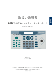
Figure 19-1 : Some of the programs with which GAMMA can easily interact. There are other
prgrams that also have been used with GAMMA, those that come to mind at the moment are SigmaPlot, Deltagraph and XMGR. These take ASCII input and need no special interface.
Scott Smith
May 22, 1998
GAMMA
Graphics & I/O
2
Gnuplot Output
Index of Figures & Tables
7
2.3
Gnuplot Output
2.1 Overview
Gnuplot is a plotting package which runs on Unix systems, PCs and Macs. It’s price (free) and versatility make it a good choice for use in visualization of data. GAMMA’s Gnuplot routines are provided to allow the output of vector, matrix, and coordinate vector data into ASCII files suitable for
plotting in Gnuplot. Aside from being able to see your simulation result plotted on virtually every
kind of computer you are using, Gnuplot also allows one to build interactive GAMMA programs
that plot to the screen. Furthermore, Gnuplot can output plots in many different formats and to
many different types of devices. More information regarding the software can be found at http://
www.cs.dartmouth.edu/gnuplot_info.html.
2.2 Available Gnuplot Functions
Functions To Make Plot Files For Gnuplot Use
GP_1D
GP_1Dm
GP_xy
GP_contour
GP_stack
- 1-Dimensional Plot
- Multiple 1-DimensionalPlots
- Parametric Plot
- Contour Plot
- Stack Plot
page 8
page 11
page 13
page 15
page 17
Functions To Make Interactive GAMMA Plots Using Gnuplot
GP_1Dplot
GP_1Dm
- 1-Dimensional Plot Interactively
- Multiple 1-DimensionalPlots
page 19
page 11
2.3 Index of Figures & Tables
Figure 4-1:
Figure 4-2:
Figure 4-3:
Figure 4-4:
Figure 4-5:
Figure 4-6:
Gnuplot Funcion GP_1D Example
Gnuplot Function GP_1Dm Example
Gnuplot Function GP_xy Example
Gnuplot Function GP_contour Example
Gnuplot Function GP_stack Example
Gnuplot 3D Spherical Plot Example
Copyright Scott A. Smith
page 10
page 12
page 14
page 16
page 18
page 22
May 22, 1998
GAMMA
Graphics & I/O
2.4
Gnuplot Output
Index of Figures & Tables
8
2.3
Routines
2.4.1
GP_1D
Usage:
#include <gnuplot.h>
void GP_1D (const char* filename, const row_vector& vx, int ri=0,
double xmin=0, double xmax=0, double cutoff=0);
void GP_1D (ofstream& ofstr, const row_vector& vx, int ri=0,
double xmin=0, double xmax=0, double cutoff=0);
Description:
The function GP_1D writes the information contained in the input row vector vx in ASCII format to either a
file or a file stream. The integer flag ri dictates whether real (ri=0, default), imaginary (ri<0), or complex values from vx will be output. If xmax or xmax & xmin are specified the horizonatal axes will be labeled, the
first point with the value of xmin and the last point with the value of xmax. For some 1D plots, points in the
Gnuplot output file may be skipped and hence (from smooth data) the output file size reduced. This is done
automatically by this GAMMA function, the value of cutoff indicative of what point variation is considered
roundoff. Note that some type of plotting do not allow for skipped points and the value of cutoff should be
left at zero. The latter form of the function is useful for successive writes of 1D spectra to the same file.
Return Value:
Nothing. A new disk file in ASCII is produced for plotting with Gnuplot (or other plotting programs which
take ASCII). It will contain either one or two plots depending on the flag “rc”.
Example:
#include <gamma.h>
main ()
{
int npts=101;
row_vector data(npts);
double x, y;
for(int i=0; i<npts; i++)
{
x = double(i-50);
y = x*x*x/125000;
x = x*x/2500;
data.put(complex(x,y),i);
}
GP_1D("real.gnu", data, 0);
GP_1D("imag.gnu", data, -1);
GP_1D("bides.gnu", data, 1);
Copyright Scott A. Smith
// How about this many points
// 1-dim. data block
// Some temporary variables
// Fill up data block
// Cubical parabolic in imaginaries
// Regular parabolic into reals
// Put this point into the vector
// Write real points to an ASCII file
// Write imaginary points to an ASCII file
// Write complex points to anASCII file
May 22, 1998
GAMMA
Graphics & I/O
Gnuplot Output
Index of Figures & Tables
9
2.3
}
When compiled and executed, the program makes three ASCII files suitable for use in Gnuplot
They may be readily viewed with that program or used in any other plotting program that takes
ASCII input. The following dialog demostrates how to display these plots on the screen on a Unix
system (assuming Gnuplot is installed and the executable “gnuplot” is in the users path).
|gamma1>gnuplot
GNUPLOT
unix version 3.5
patchlevel 3.50.1.17, 27 Aug 93
last modified Fri Aug 27 05:21:33 GMT 1993
Copyright(C) 1986 - 1993 Colin Kelley, Thomas Williams
Send comments and requests for help to info-gnuplot@dartmouth.edu
Send bugs, suggestions and mods to bug-gnuplot@dartmouth.edu
Terminal type set to 'x11'
gnuplot> set data style lines
gnuplot> plot "real.gnu"
gnuplot> plot "imag.gnu"
gnuplot> plot "bides.gnu"
gnuplot> quit
|gamma1>
Since this documentation was created with the program FrameMaker, I can also put these plots directly into the document. For example, before the “quit” command above I can do the following
gnuplot> set terminal mif
Terminal type set to 'mif'
Options are 'colour polyline'
gnuplot> set output "real.mif"
gnuplot> plot "real.gnu"
This produces three corresponding MIF files that are shown in the next figure. Other than being
resized, they have not been altered within FrameMaker (although they could be.)
Copyright Scott A. Smith
May 22, 1998
GAMMA
Graphics & I/O
Gnuplot Output
Index of Figures & Tables
10
2.3
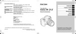
Gnuplot Funcion GP_1D Example
1
1
"real.gnu"
0.8
0.8
0.6
0.6
0.4
0.4
0.2
0.2
00
20
40
60
80
100
00
"real.gnu"
20
40
60
80
100
1
0.8
0.6
0.4
0.2
0
-0.2
-0.4
-0.6
-0.8
-10
"bides.gnu"
50
100 150 200 250
Figure 4-1 - Example program result from use of the GAMMA function “Felix”.
See Also:
Copyright Scott A. Smith
May 22, 1998
GAMMA
Graphics & I/O
2.4.2
Gnuplot Output
Index of Figures & Tables
11
2.3
GP_1Dm
Usage:
#include <gnuplot.h>
void GP_1Dm(const String& filename, row_vector* vx, int N,
int ri=0, double xmin=0, double xmax=0, int cutoff =0);
Description:
The function GP_1Dm creates an ASCII file called filename suitable for reading and plotting with Gnuplot.
It will contain plot(s) of the data contained in the array of vectors vx on the y-axis versus point number on the
x-axis. The number of vectors (in the array vx) to plot is given by the integer N. The x-axis produced will
span a range [xmin, xmax] which defaults to [0,1]. The flag “ri” dictates which plot(s) are produced. For rc
= 0 (default) only the real data is plotted. For rc < 0 only the imaginary data is plotted. For rc>0, both the real
and imaginary plots are produced. For some 1D plots, points in the Gnuplot output file may be skipped and
hence (from smooth data) the output file size reduced. This is done automatically by this GAMMA function,
the value of cutoff indicative of what point variation is considered roundoff. Note that some type of plotting
do not allow for skipped points and the value of cutoff should be left at zero.
Return Value:
Nothing. A new disk file in ASCII is produced for plotting with Gnuplot (or other plotting programs which
take ASCII). It will contain one or more plots depending on the value of N.
Example:
#include <gamma.h>
main ()
{
int i, npts=101;
row_vector data[3], datatmp(npts);
for(i=0; i<3; i++) data[i] = datatmp;
double x;
for(i=0; i<npts; i++)
{
x = double(i-npts/2);
data[0].put(x*x/2500.0,i);
data[1].put(x*x*x/12500.0,i);
data[2].put(x*x*x*x/312500.0,i);
}
GP_1Dm("plots.asc", data, 3);
cout << "\n\n";
}
Copyright Scott A. Smith
// Temp index, # points
// Vector array, temp. vector
// Initialize vectors in array
//Temp variable
// Fill up data blocks
//
//
//
//
The “x” value
The “y” value, 1st vector
The “y” value, 2nd vector
The “y” value, 3rd vector
// Write real points to ASCII file
// Keep the screen nice
May 22, 1998
GAMMA
Graphics & I/O
Gnuplot Output
Index of Figures & Tables
12
2.3
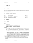
Gnuplot Function GP_1Dm Example
20
"plots.asc"
15
10
5
0
-5
-10
0
50
100
150
200
250
300
350
Figure 4-2 - Example program result from use of the GAMMA function “GP_1Dm”.
The plot above was incorporated directly into this file using the “MIF” export type in Gnuplot. After the plot is displayed on the screen, the commands set terminal MIF, set output
“plot.mif”, and replot were given to have Gnuplot produce the plot in MIF format in the
file plot.mif. The file plot.mif was imported to this document with the FrameMaker import
command under the File option.
See Also:
Copyright Scott A. Smith
May 22, 1998
GAMMA
Graphics & I/O
2.4.3
Gnuplot Output
Index of Figures & Tables
13
2.3
GP_xy
Usage:
#include <gnuplot.h>
void GP_xy (const char* filename, const row_vector &vx);
void GP_xy (ofstream& ofstr, const row_vector &vx);
Description:
The function GP_xy creates an ASCI file “filename” in a format suitible for use in Gnuplot. Unlike function
GP_1D which assumes the data is monotonically increasing on the horizontal axis, GP_xy produces plots in
parametric fashion, i.e. true x versus y. The plot will be of the data supplied by the vector vx. It is recommended that “filename” end with “.asc” to signify an ASCII file.
Return Value:
Nothing. A new disk file is produced for use in Gnuplot.
Example:
#include <gamma.h>
main ()
{
row_vector data(360);
double x,y,theta;
for(int i=0; i<360; i++)
{
theta = i*2.0*PI/360.0;
x = cos(theta);
y = sin(theta);
x = x*x*x;
y = y*y*y;
data.put(complex(x,y), i);
}
GP_xy("astroid.asc", data);
GP_xyplot("asteroid.gnu", "astroid.asc");
}
Copyright Scott A. Smith
// Create a data block
// Declare needed variables
// Loop through 360 degrees
// Fill up block with Astroid
// also called a Hypercycloid of four cusps
// x = a*[cos(theta)]**3, here a = 1
// y = a*[sin(theta)]**3, here a = 1
// Store the data point
// Output Gnuplot .mif plot file
// Interacitvely plot to screen!
May 22, 1998
GAMMA
Graphics & I/O
Gnuplot Output
Index of Figures & Tables
14
2.3
Gnuplot Function GP_xy Example
1
"astroid.asc"
0.8
0.6
0.4
0.2
0
-0.2
-0.4
-0.6
-0.8
-1
-1
-0.8
-0.6
-0.4
-0.2
0
0.2
0.4
0.6
0.8
1
Figure 4-3 - Example program result from use of the GAMMA function “GP_xy”.
The plot above was incorporated directly into this file using the “MIF” export type in Gnuplot. After the plot is displayed on the screen, the commands set terminal MIF, set output
“plot.mif”, and replot were given to have Gnuplot produce the plot in MIF format in the
file plot.mif. The file plot.mif was imported to this document with the FrameMaker import
command under the File option.
See Also: GP_1D, GP_1Dm
Copyright Scott A. Smith
May 22, 1998
GAMMA
Graphics & I/O
2.4.4
Gnuplot Output
Index of Figures & Tables
15
2.3
GP_contour
Usage:
#include <gnuplot.h>
void GP_contour(ofstream& ofstr, const row_vector& vx, double row,
int row_inc=0, double xmin=0, double xmax=0, double cutoff=0)
void GP_contour(ofstream& ofstr, matrix& mx,
int row_inc=0, double ymin=0, double ymax=0, double double xmin=0, double xmax=0)
void GP_contour(ofstream& ofstr, matrix& mx, double row,
int row_inc=0, double ymin=0, double ymax=0, double double xmin=0, double xmax=0)
Description:
The functions GP_contour is used to create contour plots in Gnuplot MIF format.
FM_contour (const char* filename, matrix &mx, double threshold, int steps, double CLI, double CLM, int
CPN, double xsize, double ysize) -The function FM_contour creates a Gnuplot file called filename in the MIF
format. The produced file will contain a contour plot of the real data contained in the matrix mx. The contours
begin at the level set by threshold and increment by the value of CLI. The number of contours is set by steps.
The levels increment either geometrically or linearly as set by the value of CLM, the default is linear. Positive
and negative contours are set by the flag CPN. For CPN=1 (default), both positive and negative contours are
produced. For CPN=0 only the positive contours are output while for CPN=-1 only the negative contours are
done. The output file contour plot will be of dimension xsize by ysize (both given in centimeters, default 10
cm).
CPN - This is a flag to indicate whether positive (or increasing), negative (or decreasing), or both positive and
negative contours. If CPN = 0, only contours increasing from the set threshold will be computed. If CPN = 1 only contours decreasing from the set threshold will be computed. If CPN = 1 (default), contour will be
computed increasing from |threshold| and decreasing from -|threshold|.
xsize, ysize - These determine the overall plot dimensions the Gnuplot output will assume. The values are
input in centimeters and are defaulted to 10 cm each. The values do nothing to the relative x to y scaling implicit in the data matrix, thus a 256 by 512 array will be 5 x 10 cm even though xsize and ysize are both set
to 10 cm.
Return Value:
Nothing. A new disk file is produced for incorporation into Gnuplot.
Copyright Scott A. Smith
May 22, 1998
GAMMA
Graphics & I/O
Gnuplot Output
Index of Figures & Tables
16
2.3
Example:
#include <gamma.h>
main()
{
matrix mx(101,101);
row_vector vx1(101), vx2(101);
vx1 = sinc(101, 50, 10);
vx2 = sin_square(101, 50);
for(int i=0; i<101; i++)
for(int j=0; j<101; j++)
mx.put(vx1.get(i)*vx2.get(j),i,j);
String afile = "contour.asc";
GP_contour(afile, mx);
GP_contplot("contour.gnu", afile);
}
// Data matrix
// Two working blocks of length 101
// Use provided window sinc function
// Use provided window sin squared function
// Loop through and fill up the matrix
// Output ASCII file name
// Write the ASCII file for Gnuplot
// Interactively output contour plot
Gnuplot Function GP_contour Example
"contour.asc"
0.797
0.595
0.392
0.189
100
-0.0135
50
0
50
0
100
Figure 4-4 - Example program result from use of the GAMMA function “GP_stack”.
See Also: FM_stack
Copyright Scott A. Smith
May 22, 1998
GAMMA
Graphics & I/O
2.4.5
Gnuplot Output
Index of Figures & Tables
17
2.3
GP_stack
Usage:
#include <gnuplot.h>
void GP_stack(ofstream& ofstr, const& row_vector, double row,
int row_inc, double xmin, double xmax, double cutoff=0)
void GP_stack(String& filename, matrix& mx,
int row_inc=0, double ymin=0, double ymax=0, double double xmin=0, double xmax=0)
void GP_stack(ofstream& ofstr, matrix& mx, double row,
int row_inc, double xmin, double xmax, double cutoff=0)
Description:
The function GP_stack creates an ASCII file Gnuplot file called “filename” in the MIF format. It contains a
single stack plot of dimension xsize by ysize (both given in centimeters, default 14 cm). The data is input in
the form of a matrix and the plot is of the entire matrix real data. The values xinc and yinc, also given in centimeters, are the amount to shift the next row in the horizontal and vertical directions respectively. The rows
which are to be plotted are specified by the value row_inc, e.g. a row increment of 3 causes the first, fourth,
seventh, etc., until the end of the matrix is reached.
Return Value:
Nothing. A new disk file is produced for incorporation into Gnuplot.
Example:
#include <gamma.h>
main()
{
matrix mx(101, 101);
row_vector vx(100);
vx = sinc(101, 50, 10);
for(int i=0; i<101; i++)
for(int j=0; j<101; j++)
mx(i,j) = vx(i) * vx(j);
String afile = "stack.asc";
GP_stack(afile, mx);
}
// Create a 101x101 matrix for data
// Create a 1D-data block of length 101
// Use provided window sinc function
// Loop through and fill up the matrix
// Output ASCII file name
// Write the ASCII file for Gnuplot
This example generates a 101x101 matrix which is a sinc function along both axes.
The following dialog demostrates how to display these plots on the screen on a Unix system (assuming Gnuplot is installed and the executable “gnuplot” is in the users path).
|gamma1>gnuplot
GNUPLOT
Copyright Scott A. Smith
May 22, 1998
GAMMA
Graphics & I/O
Gnuplot Output
Index of Figures & Tables
18
2.3
unix version 3.5
patchlevel 3.50.1.17, 27 Aug 93
last modified Fri Aug 27 05:21:33 GMT 1993
Copyright(C) 1986 - 1993 Colin Kelley, Thomas Williams
Send comments and requests for help to info-gnuplot@dartmouth.edu
Send bugs, suggestions and mods to bug-gnuplot@dartmouth.edu
Terminal type set to ’x11’
gnuplot> set data style lines
gnuplot> set parametric
gnuplot> splot "stack.asc"
Since this documentation was created with the program FrameMaker, I can also put these plots directly into the document. For example, before the “quit” command I can do the following
gnuplot> set terminal mif
Terminal type set to 'mif'
Options are 'colour polyline'
gnuplot> set output "stack.mif"
gnuplot> replot
gnuplot> quit
This produces a MIF files that is shown in the next figure. Other than being resized, is has not been
altered within FrameMaker (although it could be.)
Gnuplot Function GP_stack Example
"stack.asc"
1
0.5
0
100
-0.5
0
50
50
100
0
Figure 4-5 - Example program result from use of the GAMMA function “GP_stack”.
Copyright Scott A. Smith
May 22, 1998
GAMMA
Graphics & I/O
2.5
Gnuplot Output
Index of Figures & Tables
19
2.3
Routines for Interactive Plotting Using Gnuplot
2.5.1
GP_1Dplot
Usage:
#include <gnuplot.h>
void GP_1Dplot(const String& gnumacro, const String& file1D, int join = 1);
void GP_1Dplot(GPdat& G);
Description:
The function GP_1Dplot can be used to produce 1D plots to the screen while a GAMMA program is running
using Gnuplot. This is in three steps. First, during the course of a simulation, an ASCII file suitable for use in
Gnuplot is written to a file. Second, an ASCII file full of Gnuplot commands to plot the ASCII data file is
written to another file. Finally, Gnuplot is invoked and the commands executed.
Return Value:
Nothing. A new disk file in the MMF is produced for incorporation into Gnuplot.
Example:
#include “gamma.h”
FM_Matrix (“Testa1.mmf”,c);
}
( 6.00, 6.00)
Note that the 1,1 is set to the integer 1, the 1,2 element to 1.00 because its full
value is 1.001. The imaginary part has a value of 0.0001 and falls below threshold.
See Also: FM_Mat_Plot
Copyright Scott A. Smith
May 22, 1998
GAMMA
Graphics & I/O
2.6
Gnuplot Output
Index of Figures & Tables
20
2.3
Additional Examples
2.6.1
Spherical Plots
Description:
Although there is no function in GAMMA (yet) to support it directly, users can make 3D spherical plots with
Gnuplot and GAMMA. In this instance the program should generate a coordinate vector of the 3D points.
These are subsequently projected into 2 dimensions with the coordinate vector projection function. The
GP_xy function is then used to output the projected points.
Example:
#include <gamma.h>
main (int argc, char** argv)
{
iint N = 4096;
coord_vec data(N);
double x, y, z;
double w, W = 250.0;
double Nm1 = double(N-1);
double di;
for(int i=0; i<N; i++)
{
di = double(i);
w = W*di/Nm1;
z = -1.0 + 2.0*di/Nm1;
x = sin(w);
y = cos(w);
data.put(x,y,z,i);
}
row_vector proj(N);
double TH, PH;
double fact = 180.0/PI;
coord pt;
for(int l=0; l<N; l++)
{
pt = data(l);
TH = fact*pt.theta();
PH = fact*pt.phi();
proj.put(complex(PH,90-TH),l);
Copyright Scott A. Smith
// We’ll plot this many points
// Here’s a coordinate vector
// Here are ordinates
// Now we’ll fill up the vector
//
//
//
//
//
//
Point value
Frequency vlaue
Let z = [-1, 1]
Take x oscillating
Take y oscillating
Store coordinate
// For projected data
May 22, 1998
GAMMA
Graphics & I/O
Gnuplot Output
Index of Figures & Tables
}
GP_xy("sphere.asc", proj);
cout << "\n\n";
}
21
2.3
// 2D gnuplot of traj
// Keep the screen nice
This plot makes a helix which spirals up the surface of a sphere. The following dialog demostrates
how to display these plots on the screen on a Unix system (assuming Gnuplot is installed and the
executable “gnuplot” is in the users path).
|gamma1>gnuplot
GNUPLOT
unix version 3.5
patchlevel 3.50.1.17, 27 Aug 93
last modified Fri Aug 27 05:21:33 GMT 1993
Copyright(C) 1986 - 1993 Colin Kelley, Thomas Williams
Send comments and requests for help to info-gnuplot@dartmouth.edu
Send bugs, suggestions and mods to bug-gnuplot@dartmouth.edu
Terminal type set to 'x11'
gnuplot> set data style line
gnuplot> set parametric
dummy variable is t for curves, u/v for surfaces
gnuplot> set angles degrees
gnuplot> set title "3D Trajectory"
gnuplot> set nokey
gnuplot> set view 80,140,.6, 2.5
gnuplot> set mapping spherical
gnuplot> set samples 32
gnuplot> set isosamples 9
gnuplot> set urange [-pi/2:pi/2]
gnuplot> set vrange [0:2*pi]
gnuplot> splot cos(u)*cos(v),cos(u)*sin(v),sin(u) with lines 3 4, 'sphere.asc' with lines 1 2
gnuplot> set terminal mif
Terminal type set to 'mif'
Options are 'colour polyline'
gnuplot> set output "x.mif"
gnuplot> replot
gnuplot> quit
The last lines produce a MIF file that is shown in the next figure. Other than being resized, is has
not been altered within FrameMaker (although it could be.)
Copyright Scott A. Smith
May 22, 1998
GAMMA
Graphics & I/O
Gnuplot Output
Index of Figures & Tables
22
2.3
Gnuplot 3D Spherical Plot Example
3D Trajectory
1
0.5
0
-0.5
-0.5
-1
0
0.5
1
0.5
0
-0.5
Figure 4-6 - Example program result illustrating production of 3D spherical plots.
Copyright Scott A. Smith
May 22, 1998
GAMMA
Graphics & I/O
2.7
2.7.1
Gnuplot Output
Index of Figures & Tables
23
2.3
Additional Hints
Gnuplot Contour Plots
The contouring function takes a GAMMA matrix and slices through specified contours to produce
a Gnuplot MIF output file. An attempt is made to group all points for each specific contour line
2.7.2
Gnuplot Stack Plots
The contouring function takes a GAMMA matrix and slices through specified contours to produce
a Gnuplot MIF output file. An attempt is made to group all points for each specific contour line
Copyright Scott A. Smith
May 22, 1998
GAMMA
Graphics & I/O
3
FrameMaker Output
24
FrameMaker Output
Sections In This Document
3.1
3.2
3.3
3.4
3.5
3.6
FrameMaker Overview
Index of GAMMA’s FrameMaker Functions
Index of Figures & Tables
FrameMaker Functions
Routines for Matrix Output in FM
Mathematical Details & Code Specifics
Copyright Tilo Levante, Scott Smith, Beat H. Meier
page 25
page 26
page 26
page 27
page 54
page 58
May 22, 1998
GAMMA
Graphics & I/O
FrameMaker Output
FrameMaker Overview
25
3.1
3.1 FrameMaker Overview
The FrameMaker output routines are provided to allow the transfer of simulated plot data into
FrameMaker compatible files. This is highly useful for the preparation of documents which are to
contain plots of your GAMMA simulated spectra. FrameMaker has the ability to blend text, equations, and graphics. Using GAMMA’s FrameMaker routines, one may quickly produce publication
quality documents, transparencies, HTML pages, etc.. that contain simulated spectra directly.
Since FrameMaker also has the ability to graphically manipulate GAMMA generated files, your
plots may be cosmetically enhanced. Because GAMMA is capable of reading other file formats, it
can serve a a conversion tool. If plot files from other programs are read into GAMMA (e.g. a matrix
from Felix), they may be re-output into FrameMaker format for use in a document. FrameMaker
can also be used just for viewing GAMMA simulated spectra on the screen.
GAMMA & FrameMaker
Γ
FrameMaker
Matrix
Row Vector
Column Vector
Coordinate Vector
Figure 4-1 : GAMMA output in FrameMaker. You’re viewing a document produced with FrameMaker
and the plots were made with GAMMA.
Note that this is a one directional process! Unlike other output formats supported by GAMMA
(Felix, NMRi, etc.), GAMMA cannot re-read FrameMaker files. DO NOT make the mistake of
considering your FrameMaker output files as a means of data storage from which further mathematical manipulations may be performed within GAMMA. FrameMaker files are exclusively used
for FrameMaker.
A primary reason for GAMMA’s interface to FrameMaker is that such plots are graphic objects.
That is to say, they may be manipulated graphically inside FrameMaker. Your plots can be resized,
recolored, annotated, added into other documents, made into transparencies, etc. The downside of
this is that to use these routines you must purchase FrameMaker. More information regarding the
software can be found at http://www.frame.com.
Copyright Tilo Levante, Scott Smith, Beat H. Meier
May 22, 1998
GAMMA
Graphics & I/O
3.2
FrameMaker Output
Index of Figures & Tables
26
3.3
Index of GAMMA’s FrameMaker Functions
FM_1D
FM_1Dm
FM_xyPlot
FM_histogram
FM_scatter
FM_contour
FM_stack
FM_sphere
FM_Matrix
FM_Mat_Plot
- 1-Dimensional FrameMaker Cartesian Plot in MIF Format
- Multiple 1D FrameMaker Cartesian Plots in MIF Format
- Parametric FrameMaker Plot in MIF Format
- Histogram Plot in MIF Format
- Scatter Plot in MIF Format
- 2-Dimensional Contour Plot in MIF Format
- Stack Plot in MIF Format
- Vector(s) on a sphere plot in MIF Format
- Matrix output in MMF format
- Graphical depiction of a matrix in MIF
page 27
page 29
page 31
page 33
page 34
page 37
page 41
page 46
page 54
page 56
3.3 Index of Figures & Tables
Figure 4-1:
Figure 4-2:
Figure 4-3:
Figure 4-4:
Figure 4-4:
Figure 4-4:
Figure 4-6:
Figure 4-7:
Figure 4-7:
Figure 4-8:
Figure 4-10:
Figure 4-10:
Figure 4-11:
Figure 4-12:
Figure 4-13:
Figure 4-14:
Figure 4-15:
Figure 4-17:
Figure 4-18:
Figure 4-20:
Figure 4-20:
Figure 4-21:
Figure 4-22:
Table 1:
GAMMA Output to FrameMaker
FM_1D Example Output
FM_1Dm Example Output
XY Plot Example
Histogram Example
Size Vs. Symbol in Scatter Plots
FM_scatter Example1 Output
FM_scatter Example 2 Output
Choosing Contour Levels
Multiple Contour Levels
FM_contour Example Output
FM_stack Example Output
Euler Rotations About a and b
Euler Rotations About b and g
FM_sphere Example 1 Output
FM_sphere Example 2 Output
FM_sphere Example 3 Output
Contours
Multiple Contours
Contouring Concept
Contouring Theme
Contouring Situation
Contouring Situation
Eight (23) Triangle Based Contouring Situations Possible
Copyright Tilo Levante, Scott Smith, Beat H. Meier
page 25
page 28
page 30
page 32
page 33
page 34
page 35
page 36
page 32
page 33
page 40
page 45
page 47
page 48
page 50
page 51
page 52
page 59
page 60
page 61
page 62
page 63
page 64
page 61
May 22, 1998
GAMMA
Graphics & I/O
FrameMaker Output
FrameMaker Functions
27
3.4
3.4 FrameMaker Functions
3.4.1
FM_1D
Usage:
#include <FrameMaker.h>
void FM_1D (const char* filename, row_vector vx, double xsize=14,
double ysize=14, double min=0, double max=1, int rc=0);
Description:
The function FM_1D creates a FrameMaker file called filename in the MIF format. It will contain plot(s) of
the data contained in the vector vx on the y-axis versus point number on the x-axis. The plot(s) will be of dimension xsize by ysize in centimeters (default to 14x14 cm plot). The x-axis produced will span a range [min,
max] which defaults to [0,1]. The flag rc dictates which plot(s) are produced. For rc = 0 (default) only the
real data is plotted. For rc < 0 only the imaginary data is plotted. For rc>0, both the real and imaginary plots
are produced. FrameMaker MIF files are typically named with a “.mif” suffix so it is recommended that all
filenames used for this function end with .mif.
Return Value:
Nothing, a new disk file in the MIF is produced for incorporation into FrameMaker. It will contain either one
or two plots depending on the flag “rc”.
Example:
#include <gamma.h>
main ()
{
row_vector vx(101);
double x, y;
for(int i=0; i<101; i++)
{
x = double(i-50);
y = x*x*x/125000;
x = x*x/2500;
vx.put(complex(x,y),i);
}
FM_1D(“FM.mif”,BLK,10,5, -50, 50, 1);
}
Copyright Tilo Levante, Scott Smith, Beat H. Meier
// Block for data points
// Working x,y ordinates
// Fill up data block
// Offset x (so centered)
// Cubical parabolic (imag)
// Parabolic into reals
// Store this point
// Output FM.mif, both plots
May 22, 1998
GAMMA
Graphics & I/O
FrameMaker Output
FrameMaker Functions
28
3.4
FM_1D Example Output
1
1
0.8
0.5
0.6
0
0.4
-0.5
0.2
0
-1
-40
-20
0
20
40
-40
-20
0
20
40
Figure 4-2 - The two plots above were contained in the file FM.mif and imported directly to
this document without further alteration. The import command within FrameMaker is
under the File option. These plots were produced from the example code.
See Also: FM_1Dm, FM_xyPlot, FM_scatter, FM_histogram
Copyright Tilo Levante, Scott Smith, Beat H. Meier
May 22, 1998
GAMMA
Graphics & I/O
3.4.2
FrameMaker Output
FrameMaker Functions
29
3.4
FM_1Dm
Usage:
#include <FrameMaker.h>
void FM_1Dm(const char* filename, int N, row_vector* vxs);
Description:
The function FM_1Dm creates a FrameMaker file called filename in MIF format. It will contain plots of the
data contained in the N vectors which are pointed to by vxs These plot(s) may be further manipulated from
within FrameMaker itself. FrameMaker MIF files are typically named with a “.mif” suffix so it is recommended that all filenames used for this function end with .mif.
Return Value:
Nothing. A new disk file in the MIF is produced for incorporation into FrameMaker. It will contain either one
or two plots depending on the flag “rc”.
Example:
#include <gamma.h>
main()
{
int i, j, N=5;
row_vector vxs[5], vx(101);
for(i=0; i<N; i++) vxs[i] = vx;
double x;
for(i=0; i<101; i++)
{
x = double(i-50);
x = x*x/2500;
for(j=0; j<N; j++)
vxs[j].put(complex(j*x),i);
}
FM_1Dm("FM.mif", N, vxs);
}
Copyright Tilo Levante, Scott Smith, Beat H. Meier
// This many plots
// Blocks for data points
// Initilize the 5 blocks
// Working x,y ordinates
// Fill up data blocks
// Offset x (so centered)
// Parabolic function
// Store this point
// Output to FM.mif, N plots
May 22, 1998
GAMMA
Graphics & I/O
FrameMaker Output
FrameMaker Functions
30
3.4
FM_1Dm Example Output
4
3
2
1
0
0
0.2
0.4
0.6
0.8
1
Figure 4-3 - The two plots above were contained in the file FM.mif and imported directly to
this document. I did some coloring, resizing, and a bit of axis adjusting in FrameMaker.
The import command within FrameMaker is under the File option. These plots were produced from the example code.
See Also: FM_1D, FM_xyPlot, FM_scatter, FM_histogram
Copyright Tilo Levante, Scott Smith, Beat H. Meier
May 22, 1998
GAMMA
Graphics & I/O
3.4.3
FrameMaker Output
FrameMaker Functions
31
3.4
FM_xyPlot
Usage:
#include <FrameMaker.h>
void FM_xyPlot (const char* filename, row_vector &vx, double xsize=14, double ysize=14);
Description:
The function FM_xyPlot creates a FrameMaker file “filename” in the MIF format. Unlike function FM_1D
which assumes the data monotonically increasing on the horizontal axis, FM_xyPlot produces plots in parametric fashion, i.e. true x versus y. The plot will be of the data supplied by the vector vx and the plot dimension
xsize by ysize in centimeters (default to 14x14 cm plot). It is recommended that “filename” end with “.mif”
to signify a FrameMaker MIF file. Note: block_1D can be substituted for row_vector in the function call here.
Return Value:
Nothing. A new disk file is produced for incorporation into FrameMaker.
Example:
#include <gamma.h>
main ()
{
block_1D BLK(360);
double x,y,theta;
for(int i=0; i<360; i++)
{
theta = i*2.0*PI/360.0;
x = cos(theta);
y = sin(theta);
x = x*x*x;
y = y*y*y;
BLK(i) = complex(x,y);
}
FM_xyPlot(“astroid.mif”, BLK);
}
Copyright Tilo Levante, Scott Smith, Beat H. Meier
// create a data block
// declare needed variables
// loop through 360 degrees
// fill up block with Astroid
// also called a Hypercycloid of four cusps
// x = a*[cos(theta)]**3, here a = 1
// y = a*[sin(theta)]**3, here a = 1
// output FrameMaker .mif plot file
May 22, 1998
GAMMA
Graphics & I/O
FrameMaker Output
FrameMaker Functions
32
3.4
XY Plot Example
1
0.5
0
-0.5
-1
-1
-0.5
0
0.5
1
Figure 4-4 - The two plots above were contained in the file FM.mif and imported directly to
this document without further alteration. The import command within FrameMaker is
under the File option. These plots were produced from the example code.
See Also: FM_1D, FM_1Dm, FM_scatter, FM_histogram
Copyright Tilo Levante, Scott Smith, Beat H. Meier
May 22, 1998
GAMMA
Graphics & I/O
3.4.4
FrameMaker Output
FrameMaker Functions
33
3.4
FM_histogram
Usage: **** Note this function works but is still under construction. It may fail if the number of points
does not far exceed the number of bins (a factor of >100 seems o.k.)
#include <FrameMaker.h>
void FM_histogram (const char* filename, row_vector &vx, int bins = 0,
double xsize=14, double ysize=14);
Description:
The function FM_histogram creates a FrameMaker file called “filename” in the MIF format The plot will be
of the data supplied by the vector vx and the plot dimension xsize by ysize in centimeters (default to 14x14
cm plot). The number of bins is specified by the integer “bins” and should not exceed the number of points
in the input data vector. The default number is zero whereupon each point in vx is a separate bin. Currently
the data must be increasing monotonic. It is recommended that “filename” end with “.mif” to signify a
FrameMaker MIF file. Note: block_1D can be substituted for row_vector in the function call. Each bin of the
histogram may be manipulated individually within FrameMaker.
Return Value:
Nothing. A new disk file is produced for incorporation into FrameMaker.
Example:
#include <gamma.h>
main ()
{
row_vector vx(51);
// create a data block
row_vector vx1(51);
//
vx1 = Gaussian(51, 25, 3);
// fill up data with Gaussian
for(int i=0; i<51; i++)
vx(i) = complex(i, Re(vx1(i)));
FM_histogram(“FM.mif”, vx, bins); // output FrameMaker .mif plot file
}
Histogram Example
1
0.8
0.6
0.4
0.2
0
10
20
30
40
50
See Also: FM_1D, FM_1Dm, FM_xyPlot, FM_scatter
Copyright Tilo Levante, Scott Smith, Beat H. Meier
May 22, 1998
GAMMA
Graphics & I/O
3.4.5
FrameMaker Output
FrameMaker Functions
34
3.4
FM_scatter
Usage:
#include <FrameMaker.h>
void FM_scatter (const char* filename, row_vector &vx, int sides=0,
double PGsize=0, double xsize=14, double ysize=14);
void FM_scatter (const char* filename, row_vector &vx, char a=’o’,
double xsize=14, double ysize=14);
Description:
The function FM_scatter is essentially the same as the function FM_xyPlot except that the points are not connected by a line, they are marked with a specified symbol. The FrameMaker MIF file “filename” is created
containing a plot of the data supplied by the vector vx. The plot dimension is xsize by ysize in centimeters
(default to 14x14 cm plot). The data is plotted x versus y where x are the real points of the vector and y the
imaginary points.
1.
FM_scatter (const char* filename, row_vector &vx, int sides=0, double PGsize=0, double xsize=14,
double ysize=14) - When the function is called with these arguments a graphic object is used to mark the
point in the scatter plot. The size of the symbol is given in centimeters by “PGsize” which defaults to 1/
100 of xsize. PGsize is the radius of the circle which circumscribes the graphics objects marking the
points. The object itself is determined by the value of “sides”. Typically “sides” will be the number of
sides of a polygon and defaults to zero in order to indicate a circle. The following are valid numbers for
“sides”
Size Vs. Symbol in Scatter Plots
size
object
size
object
size
<-3
[0,2]
6
-3
3
7
-2
4
8
-1
5
>8
object
Figure 4-5 - Value of “size” vs. Symbol Output. These may also be set inside FrameMaker..
The objects shown above were taken from plots made with the FM_scatter function using the various size
values and 0.25 for PGsize.
2.
FM_scatter (const char* filename, row_vector &vx, char a, double xsize=14, double ysize=14) - When
the function is called with these arguments it uses a character to mark the points in the scatter plot.
These objects marking the plotted points are grouped together and can be manipulated as a whole or individually inside of FrameMaker. It is recommended that “filename” end with “.mif” to signify a FrameMaker MIF
file. Note: block_1D can be substituted for row_vector in this function.
Return Value:
Nothing. A new disk file is produced for incorporation into FrameMaker.
Copyright Tilo Levante, Scott Smith, Beat H. Meier
May 22, 1998
GAMMA
Graphics & I/O
FrameMaker Output
FrameMaker Functions
35
3.4
Examples:
#include <gamma.h>
main ()
{
block_1D BLK(50);
double x,y,theta;
double a,b;
for(int i=0; i<50; i++)
{
a = 1;
b = 2;
theta = -PI + i*(4.0*PI/49.0);
x = a*theta - b*sin(theta);
y = a - b*cos(theta);
BLK(i) = complex(x,y);
}
FM_scatter(“FM.mif”, BLK, 0,.1, 14, 5);
}
// create a data block
// declare needed variables
// declare needed variables
// loop through 50 points
// fill up block with Prolate Cycloid
// angles span -pi to 3pi
// x = a(theta) - b*sin(theta), here a=1, b=2
// y = a - b*cos(theta)
// output FrameMaker .mif plot file
FM_scatter Example1 Output
3
2
1
0
-2
0
2
4
6
8
Figure 4-6 - The plot above was contained in the file FM.mif and imported directly to this
document. Minor alterations were performed in FrameMaker (coloring, sizing, and axis
font changes). The import command within FrameMaker is under the File option. Each
symbol can be manipulated individually or all simultaneously within FrameMaker.
Thus one can fill the circles, change their sizes, etc. after the plot has been produced.
The next example demonstrates this ability and the use of characters to mark the points.
Copyright Tilo Levante, Scott Smith, Beat H. Meier
May 22, 1998
GAMMA
Graphics & I/O
FrameMaker Output
FrameMaker Functions
#include <gamma.h>
main ()
{
block_1D BLK(101);
double x,y,a=3;
for(int i=0; i<51; i++)
{
x = (5.5*i/50)-2.5;
y = sqrt(x*x*(a-x)/(a+x));
BLK(i) = complex(x,y);
BLK(100-i) = complex(x,-y);
}
FM_scatter(“FM.mif”, BLK, ‘b’);
points.
}
36
3.4
// create a data block
// declare needed variables
// fill block with Strophoid
// y**2 = x**2[(a-x)/(a+x)]
// Output FM scatter plot, letter b marking
FM_scatter Example 2 Output
b
b
b
5
b
bb
bb
bb
bbb
0
-5
b
b
b
b
b
bb
-2
b
bb
bb
bbbb
bb
bbb bbbbbb bb b b b b
bbbbb
b bb bb bb bb b b bb bb
bb
b
b
b
b
b
b
bbbbbbbbbbbbbbbbbbbbbb
b
b
b
b
b
-1
0
1
2
3
Figure 4-7 This plot above was also produced into a file called FM.mif and imported directly to this
document. It has be subsequently altered within Framemaker. First, the overall plot dimensions
was changed from the default values of 14cm by 14cm. Second, the plot originally had the character b marking each point. As all points are a single graphics object these b’s were all changed
simultaneously to a larger font size (default 12pt to 14pt) and to a new font type (Zapfdingbat).
See Also: FM_1D, FM_1Dm, FM_xyPlot, FM_histogram
Copyright Tilo Levante, Scott Smith, Beat H. Meier
May 22, 1998
GAMMA
Graphics & I/O
3.4.6
FrameMaker Output
FrameMaker Functions
37
3.4
FM_contour
Usage:
#include <FrameMaker.h>
void FM_contour(const char* filename, matrix &mx, double threshold, int steps=3,
double CLI=0, double CLM=1, int CPN=1, double xsize=10, double ysize=10);
Description:
The functions FM_contour is used to create contour plots in FrameMaker MIF format.
FM_contour (const char* filename, matrix &mx, double threshold, int steps, double CLI, double CLM, int
CPN, double xsize, double ysize) -The function FM_contour creates a FrameMaker file called filename in the
MIF format. The produced file will contain a contour plot of the real data contained in the matrix mx. The
contours begin at the level set by threshold and increment by the value of CLI. The number of contours is set
by steps. The levels increment either geometrically or linearly as set by the value of CLM, the default is linear.
Positive and negative contours are set by the flag CPN. For CPN=1 (default), both positive and negative contours are produced. For CPN=0 only the positive contours are output while for CPN=-1 only the negative contours are done. The output file contour plot will be of dimension xsize by ysize (both given in centimeters,
default 10 cm).
Contour Parameters filename - Although not mandatory, this should be “name.mif” where the .mif indicates a FrameMaker file.
mx - Can be any matrix or block_2D in GAMMA. Note that it is the real data that is contoured.
threshold - This can be a positive or negative quantity. If both positive and negative contours are to be performed, the absolute value will be taken for the first contour of the positives and the negative of the absolute
value taken as the first contour of the negative levels. This is shown in the following figure where the dashed
line indicates the value of threshold and the arrows indicate the direction of subsequent contour levels.
Choosing Contour Levels
1
0.8
0.6
0.4
0.2
0
-0.2
1
0.8
0.6
0.4
0.2
0
-0.2
CPN = 0
threshold = -0.1
1
0.8
0.6
0.4
0.2
0
-0.2
CPN = -1
threshold = 0.6
CPN = 1
threshold = +/-0.1
Figure 4-8 - Depiction of the two basic parameters for picking contour levels.
steps - This is the number of contour levels to plot. The default value is 3 and the maximum value is set to 20.
If both positive and negative contours are output, there will be still be this number performed in both contour
directions. Note that the contours may not be visible in the plot if there is no data in the input matrix corresponding to the contour level.
CLI, CLM - These are the linear and geometric factors which change the contour levels at each step. CLI must
Copyright Tilo Levante, Scott Smith, Beat H. Meier
May 22, 1998
GAMMA
Graphics & I/O
FrameMaker Output
FrameMaker Functions
38
3.4
have a positive value regardless of whether one desires positive or negative contours. CLM must be positive
and >= 1. Typically CLM ranges between 1(default) and 2. The first contour will occur at the value set by
threshold (level 0 = threshold). The next contour will be determined strictly by the threshold value and the
value of CLI, namely level 1 = threshold + CLI. Subsequent levels are determined jointly by the values of
CLM (Contour Level Modifier) and CLI (Contour Level Increment). Generally the contour levels above the
initial level 0 are determined from level i = level (i-1) + [CLI * (CLM)i-1]. Note that there is a default setting
of CLI to zero which flags the contour function(s) to determine an appropriate CLI for the number of steps
input. Below are a few 1-dimensional plots depicting how CLM and CLI interact. Setting CPN to -1 would
will keep the contour spacing the same but they will decrease in height from the initial level.
Multiple Contour Levels
1
0.8
0.6
0.4
0.2
0
-0.2
threshold = -0.1
steps >= 11
CLI = 0.1
CLM = 1
CPN = 0
1
0.8
0.6
0.4
0.2
0
-0.2
threshold = 0
steps >= 3
CLI = 0.3
CLM = 1
CPN = 0
1
0.8
0.6
0.4
0.2
0
-0.2
threshold = -0.1
steps >= 5
CLI = 0.1
CLM = 1.5
CPN = 0
Figure 4-9 - Examples depicting function arguments vs. contour levels chosen..
Setting CPN to 1 will produce the same levels as well as those mirrored vertically about 0, except that the
input threshold must be greater than 0. Thus keeping the setting as in the above diagram the but with CPN=1
will force the function to internally alter these input thresholds.
CPN - This is a flag to indicate whether positive (or increasing), negative (or decreasing), or both positive and
negative contours. If CPN = 0, only contours increasing from the set threshold will be computed. If CPN = 1 only contours decreasing from the set threshold will be computed. If CPN = 1 (default), contour will be
computed increasing from |threshold| and decreasing from -|threshold|.
xsize, ysize - These determine the overall plot dimensions the FrameMaker output will assume. The values
are input in centimeters and are defaulted to 10 cm each. The values do nothing to the relative x to y scaling
implicit in the data matrix, thus a 256 by 512 array will be 5 x 10 cm even though xsize and ysize are both set
Copyright Tilo Levante, Scott Smith, Beat H. Meier
May 22, 1998
GAMMA
Graphics & I/O
FrameMaker Output
FrameMaker Functions
39
3.4
to 10 cm.
Return Value:
Nothing. A new disk file is produced for incorporation into FrameMaker.
Copyright Tilo Levante, Scott Smith, Beat H. Meier
May 22, 1998
GAMMA
Graphics & I/O
FrameMaker Output
FrameMaker Functions
40
3.4
Example:
#include <gamma.h>
main()
{
matrix mx(101, 101);
row_vector BLK1 = sinc(101, 50, 10);
row_vector BLK2 = sin_square(101, 50);
for(int i=0; i<101; i++)
for(int j=0; j<101; j++)
mx(i,j) = BLK1(i) * BLK2(j);
FM_contour(“contour.mif”,mx,.05,10,.05);
}
// create a 101x101 matrix for data
// use provided window sinc function
// use provided window sin squared function
// loop through and fill up the matrix
//create file FM contour file - contour.mif
FM_contour Example Output
1
0.8
0.6
0.4
0.2
0
-0.2
0.8
0.6
0.4
0.2
0
Figure 4-10 Contour plot of the 101x101 matrix which is a sin2(x) on one axis and a sinc(y) on the
other axis. The first contour is set at +/-0.05 and increments by 0.05 up and down over 10 contours - of which only four of the negative contours exist. The file contour.mif was incorporated
directly (contained in the box) to this document using the FrameMaker import command. The
plot was resized and the negative contour lines switched to dashed for highlighting. The two
1D-plots were independently generated (with FM_1D) and added for clarity.
See Also: FM_stack
Copyright Tilo Levante, Scott Smith, Beat H. Meier
May 22, 1998
GAMMA
Graphics & I/O
3.4.7
FrameMaker Output
FrameMaker Functions
41
3.4
FM_stack
Usage:
#include <FrameMaker.h>
void FM_stack(const char* filename, matrix &mx, double xinc, double yinc,
int row_inc, double xsize=14, double ysize=14)
Description:
The function FM_stack creates a FrameMaker file called “filename” in the MIF format. It contains a single
stack plot of dimension xsize by ysize (both given in centimeters, default 14 cm). The data is input in the form
of a matrix and the plot is of the entire matrix real data. The values xinc and yinc, also given in centimeters,
are the amount to shift the next row in the horizontal and vertical directions respectively. The rows which are
to be plotted are specified by the value row_inc, e.g. a row increment of 3 causes the first, fourth, seventh,
etc., until the end of the matrix is reached.
Plotting Parameters - The total plot dimension is specified by the values of xsize and ysize, the entire plot
will be scaled to fit into this box. The amount of skewing that the plane containing the baselines, i.e. where
the zero level of the rows lie, is set by the values of xinc and yinc. This plane is that which is horizontally
striped in the figure. The value of ∆x is (mxrows+1)*xinc and the value of ∆y is (mxrows+1)*yinc where
mxrows are the total number of rows in the input matrix. (The 1 is added because there is a border drawn
around the plane). Peak intensities will then be scaled to fill the rest of the plot area. Thus, vertical peak scaling is mainly determined by combination of yinc and ysize.
Stack Plot Perspective
∆y
ysize
∆x
xsize
Figure 4-11 - How to set the skew or viewing angle in the FM stack plot function.
Changes made to the row increment, row_inc, somewhat affects plot scaling as well because only the rows
actually plotted are considered, not the entire data matrix input. The figure below demonstrates the effect of
increasing the value of row_inc.
Copyright Tilo Levante, Scott Smith, Beat H. Meier
May 22, 1998
GAMMA
Graphics & I/O
FrameMaker Output
FrameMaker Functions
42
3.4
Stack Plot Row Increments
increased
row_inc
Figure 4-12 - The effect of the row increment arguemnt.
The value of xinc dictates how much horizontal skew there is in the final plot. Negative values are acceptable,
this simply changes the orientation as shown in the next figure.
Negative xinc
Zero xinc
Positive xinc
Larger Positive
Figure 4-13 - How xinc affects the skewing of the output stack plot.
In a similar fashion, yinc dictates the amount of vertical skew there is. Negative values for yinc are not currently supported and will yield unpredictable plots. Rather it is recommended that the matrix is multiplied by
-1 prior to entering this function.
xinc, yinc, and Stack Plots
Not supported
Negative yinc
Zero yinc
Positive yinc
Larger Positive
Figure 4-14 - How xinc affects the skewing of the output stack plot.
Graphics Properties - Within FrameMaker, stack plots generated with this function are full graphics objects and have
a graphics hierarchy. The entire plot is grouped and can be resized, annotated, or rotated. As a example, the figure below is a stack plot generated with this function which has been manipulated several different ways within FrameMaker.
Copyright Tilo Levante, Scott Smith, Beat H. Meier
May 22, 1998
GAMMA
Graphics & I/O
FrameMaker Output
FrameMaker Functions
43
3.4
Graphical Manipulations of Stack Plots Within FrameMaker
.
Rescaled
Original Plot
Hidden Lines now Visible
Rotated
Figure 4-15 - The two plots above were contained in the file FM.mif and imported directly
to this document without further alteration. The import command within FrameMaker
is under the File option. These plots were produced from the example code.
Furthermore, each row can be individually manipulated also be manipulated as a graphics object as the following diagram illustrates.
Copyright Tilo Levante, Scott Smith, Beat H. Meier
May 22, 1998
GAMMA
Graphics & I/O
FrameMaker Output
FrameMaker Functions
44
3.4
More Graphical Manipulations of Stack Plots
Original Plot
Specific Line Highlighted
Positive, in plane, & negative
Specific Line Isolated
Figure 4-16 - The two plots above were contained in the file FM.mif and imported directly
to this document without further alteration. The import command within FrameMaker
is under the File option. These plots were produced from the example code.
FrameMaker MIF files are typically named with a “.mif” suffix so it is recommended that all filenames used
for this function have a .mif at the end.
Return Value:
Nothing. A new disk file is produced for incorporation into FrameMaker.
Example:
#include <gamma.h>
main()
{
matrix mx(101, 101);
block_1D vx(100);
vx = sinc(101, 50, 10);
for(int i=0; i<101; i++)
for(int j=0; j<101; j++)
mx(i,j) = vx(i) * vx(j);
FM_stack(“stack.mif”, mx, 0.02, 0.02, 1);
}
Copyright Tilo Levante, Scott Smith, Beat H. Meier
// create a 101x101 matrix for data
// create a 1D-data block of length 101
// use provided window sinc function
// loop through and fill up the matrix
// output the FrameMaker .mif plot file
May 22, 1998
GAMMA
Graphics & I/O
FrameMaker Output
FrameMaker Functions
45
3.4
FM_stack Example Output
Figure 4-17 This example generates a 101x101 matrix which is a sinc function along both axes. The
first contour block plotted is row 0. Each successive row begins 0.02 cm above and 0.02 over
from the previous row. In this example the row increment is set to 7. The default dimensions of
14x14 cm are used (because they are left out of the function call). Note that the plot here has
been rescaled.
See Also: FM_contour
Copyright Tilo Levante, Scott Smith, Beat H. Meier
May 22, 1998
GAMMA
Graphics & I/O
3.4.8
FrameMaker Output
FrameMaker Functions
46
3.4
FM_sphere
Usage:
#include <FrameMaker.h>
void FM_sphere(const char* filename, int type=2, double alpha=0, double beta=15,
double gamma=-15, double radius=5, double points=100);
void FM_sphere(const char* filename, coord_vec &data, int type=0, double alpha=0,
double beta=15, double gamma=-15, double radius=5, double points=100);
void FM_sphere(const char* filename, coord_vec &data1, coord_vec &data2, int type=0,
i double alpha=0, double beta=15, double gamma=-15, double radius=5, double points=100);
Description:
The function FM_sphere creates a FrameMaker file called filename in the MIF format. It contains a single
3D-plot which has been projected after rotation by the Euler angles alpha, beta, and gamma (input in degrees)
to produce the desired perspective.
1.
FM_sphere (const char* filename, int type, double alpha, double beta, double gamma, double radius, int
points) - Used in this manner, the function plots no data, only coordinate axes and/or a coordinate sphere
depending on the value of type. For type = 0, the three coordinate axes are drawn of (unprojected) length
2*radius. For type=0, the coordinate sphere having radius of radius is drawn along with it’s intersection
with the three planes (xy, xz, & yz). For type = 2, both the axes and the sphere are drawn. The value of
points specifies how many points to use when drawing each sphere-plane intersection.
2.
FM_sphere (const char* filename, double coord_vec, int type, double alpha, double beta, double gamma,
double radius, int points) - When the function is called with these arguments it draws the plot produced
in the description above (1.) with both axes and the coordinate sphere. It then adds the data contained in
the coord_vec data to the plot.
3.
FM_sphere (const char* filename, double coord_vec, double coord_vec, int type, double alpha, double
beta, double gamma, double radius, int points) - When the function is called with these arguments is the
same as the previous description (2.) but plots both data sets, data1 and data2.
2D Projection - Initially, the coordinates and/or drawn coordinate system is rotated by the specified Euler angles. The
rotated three dimensional coordinates are then projected onto the 2D plane of the paper (or screen). To produce a reasonable plot the 3D z-coordinates is mapped into the 2D y-coordinates and the 3D x-coordinates are mapped into the
2D negative x-coordinate as depicted in the figure below. This mapping keeps everything related to standard righthanded coordinate systems. The initial, unrotated system has y coming up out of the paper plane.
Figure 4-18 - Depiction of (simple) 3D Euler Rotation and subsequent projection on plot axes.
Perspective, Euler Rotations - The three Euler angles can dramatically change the quality of the out put plot. The default Euler angles are set to produce a nice view of typical data, maintaining the z axis vertical. The following figures
demonstrate by example the effect of the various Euler angles on the final coordinate axes in which the data is drawn.
Copyright Tilo Levante, Scott Smith, Beat H. Meier
May 22, 1998
GAMMA
Graphics & I/O
FrameMaker Output
FrameMaker Functions
z
47
3.4
y
Z
α, β, γ
x
project
X
y
x
Y
Coordinate Vector
Coordinate System
Rotated Data
Coordinate System
2D Projected (Paper)
Coordinate System
Euler Rotations About α and β
z
z
α=0
β=0
α=10
β=0
z
z
x
x
α=0
β=10
z
x
y
y
α=10
β=45
y
α=0
β=45
x
y
α=0
β=90
α=90
β=0
z
x
y
z
y
α=45
β=10
α=90
β=10
z
z
x
x
x
α=45
β=0
α=10
β=10
z
z
y
x,y
x
x
z
y
α=45
β=45
α=90
β=45
z
x,z
y
α=10
β=90
y
y
α=45
β=90
y
α=90
β=90
Figure 4-19 - Examples of rotations using only the 1st two Euler Angles.
Copyright Tilo Levante, Scott Smith, Beat H. Meier
May 22, 1998
GAMMA
Graphics & I/O
FrameMaker Output
FrameMaker Functions
48
3.4
These axes were generated with the program listed as Example 1 using a radius of 1 (cm), a gamma value of zero (degrees), and type 0 (only axes). The axis orientation proceeds via first rotating about the z axis with angle alpha followed
by rotation about the new x axis with angle beta. The last rotation, if gamma were non-zero, is about the new z axis
with angle gamma. Looking from the positive axis toward the origin, all rotations appear clock-wise1.
Euler Rotations About β and γ
z
x
z
z
x
x
β=0
γ=0
β=10
γ=0
z
z
y
β=45
γ=0
y
x
y
β=0
γ=10
β=10
γ=10
z
z
y
β=90
γ=10
β=45
γ=10
x
x
y
x,y
y
β=90
γ=0
z
x
x
x
x
z
x
y
β=0
γ=45
β=10
γ=45
z
z
y
y
y
β=45
γ=45
x
z
y
β=90
γ=45
y
x
β=0
γ=90
β=10
γ=90
β=45
γ=90
β=90
γ=90
Figure 4-20 Again, these axes were generated with the program listed as Example 1. The axis ori1. Euler rotations follow the right hand rule, that is, the coordinate system moves counter-clockwise about the
rotation axes. An alternate and equivalent view is that the coordinates themselves move clock-wise about stationary axes. This function strictly adheres to this convention. The overall plot is reference to some static axes.
Any data is thus rotates by input Euler angles clock-wise relative to these stationary axes. The axes sketched
by this function are axes for the data (absent in one function usage) of the input coordinate vector, not the
overall static reference axis. Thus, the rotations of the plotted axes follow the rotation convention of the coordinates themselves: they rotate clockwise about the axes of rotation.
Copyright Tilo Levante, Scott Smith, Beat H. Meier
May 22, 1998
GAMMA
Graphics & I/O
FrameMaker Output
FrameMaker Functions
49
3.4
entation proceeds via first rotating about the z axis with angle alpha (in this case alpha=0, so
not performed), followed by rotation about the new x axis with angle beta (in this case about the
original x-axis), and then followed by rotation about the new z axis with angle gamma.Looking
from the positive axis toward the origin, all rotations appear clock-wise.
Copyright Tilo Levante, Scott Smith, Beat H. Meier
May 22, 1998
GAMMA
Graphics & I/O
FrameMaker Output
FrameMaker Functions
50
3.4
Example 1:
#include <gamma.h>
main ()
{
cout << “\nPlease input a radius(cm): “;
double radius;
cin >> radius;
cout << “\nPlease input a Euler angle alpha(deg): “;
double alpha;
cin >> alpha;
cout << “\nPlease input a Euler angle beta(deg): “;
double beta;
cin >> beta;
cout << “\nPlease input a Euler angle gamma(deg): “;
double gamma;
cin >> gamma;
cout << “\nPlease input plot type (0=axes, 1=planes, 2=both): “;
int type;
cin >> type;
FM_sphere(“FM_sph1.mif”, type, alpha, beta, gamma, radius);
}
FM_sphere Example 1 Output
α = 45
β = 10
γ=0
type = 0
radius = 2
α=5
β = 10
γ = 15
type = 1
radius = 1.0
α=0
β = 15
γ = −15
type = 2
radius = 1.5
Figure 4-21 This example program runs interactively and prompts the user for information concerning the plot. Here, the function FM_sphere is used only to produce a coordinates system plot either axes, the coordinates sphere, or both.
Copyright Tilo Levante, Scott Smith, Beat H. Meier
May 22, 1998
GAMMA
Graphics & I/O
FrameMaker Output
FrameMaker Functions
51
3.4
Example 2:
#include <gamma.h>
main ()
{
coord_vec data1(500);
coord_vec data2(500);
double xx, yy, zz;
double theta;
for(int i=0; i<500; i++)
{
theta = i*6.0*PI/499.0;
xx = 3.0*cos(theta);
yy = 3.0*sin(theta);
zz = 3.0 - (6.*i/499.);
data1.put(xx, yy, zz, i);
}
data2 = data1.rotate(90,90,0);
FM_sphere(“FM_sph2a.mif”, data1,0);
FM_sphere(“FM_sph2b.mif”, data2,1);
}
// Declare a 500 point coordinate vector
// A second coordinate vector
// Declare needed variables
// Declare an angle variable
// Fill data1 with a spiral
// Set 2nd coordinate vector to rotated data1
// Output FrameMaker file FM_sph2a.mif
// Output FrameMaker file FM_sph2b.mif
FM_sphere Example 2 Output
Figure 4-22 This example demonstrates the use of the function FM_sphere for plotting a coordinate
vector. The value of type indicates whether the plotted data should be a solid line, individual
points, or vectors (see Example 3). The function rotate is a member function of a coordinate
vector. The sphere size (default 5 cm radius) was altered to 2.5 cm radius within FrameMaker.
Copyright Tilo Levante, Scott Smith, Beat H. Meier
May 22, 1998
GAMMA
Graphics & I/O
FrameMaker Output
FrameMaker Functions
52
3.4
Example 3:
#include <gamma.h>
main ()
{
int size = 31;
// Set 31 points
coord_vec traj1(size);
// Declare two coordinate vectors
coord_vec traj2(size);
double xx, yy, theta;
for(int i=0; i<size; i++)
// Fill coordinate vectors
{
// Trajectory 1 is in the yz plane
theta = (PI/2.0)*i/(size-1);
// decreasing from (001) to (010)
xx = cos(theta);
// Trajectory 2 is in the xz plane
yy = sin(theta);
// decreasing from (100) to (00-1)
traj1.put(0,yy,xx,i);
traj2.put(xx,0,-yy,i);
}
FM_sphere(“FM_sph2.mif”, traj1, // Output FrameMaker MIF file
traj2, 2, 0.0, 15.0, -45.0); // Euler angles for nice perspective
}
FM_sphere Example 3 Output
Figure 4-23 - The two plots above were contained in the file FM.mif and imported directly
Copyright Tilo Levante, Scott Smith, Beat H. Meier
May 22, 1998
GAMMA
Graphics & I/O
FrameMaker Output
FrameMaker Functions
53
3.4
to this document without further alteration. The import command within FrameMaker
is under the File option. These plots were produced from the example code.
See Also: None
Copyright Tilo Levante, Scott Smith, Beat H. Meier
May 22, 1998
GAMMA
Graphics & I/O
3.5
FrameMaker Output
FrameMaker Functions
54
3.4
Routines for Matrix Output in FM
3.5.1
FM_Matrix
Usage:
#include <FrameMaker.h>
void FM_Matrix (const char* filename, gen_op& Op, int prec = 2, int threshold = 0.001);
void FM_Matrix (const char* filename, matrix& mx, int prec = 2, int threshold = 0.001);
Description:
The function FM_Matrix generates a FrameMaker Mathematical Language (MML) file which can be directly imported into a FrameMaker Document. For floating numbers, prec (default=2) digits after the decimal
point will be used. If either the real or imaginary part has a norm of lower than threshold, it will be left away
on output. If both, the real and imaginary part are below threshold, a simple 0 is written to Output.
If a floating number is closer then threshold to the nearest integer, the integer is outputed.(See example below).
Return Value:
Nothing. A new disk file in the MMF is produced for incorporation into FrameMaker.
Example:
#include “gamma.h”
main()
{
matrix c;
cin >> c;
cout << c;
FM_Matrix (“Testa1.mmf”,c);
}
Dialog From Program Execution:
>3 3
>1.0 0.0
>1.001 0.0001
>0 0.00001
>0 .1
.>1 0
>5 3.00001
>4 4
>5 5
>6 6
3 x 3 full matrix
Copyright Tilo Levante, Scott Smith, Beat H. Meier
May 22, 1998
GAMMA
Graphics & I/O
FrameMaker Output
FrameMaker Functions
55
3.4
( 1.00, 0.00) ( 1.00, 0.00) ( 0.00, 0.00)
( 0.00, 0.10) ( 0.10, 0.00) ( 5.00, 3.00)
( 4.00, 4.00) ( 5.00, 5.00) ( 6.00, 6.00)
Testa1.mmf file imported directly into this document:
1
1.00
0
0.10 ⋅ i
0.10 ( 5 + 3 ⋅ i )
(4 + 4 ⋅ i) (5 + 5 ⋅ i) (6 + 6 ⋅ i)
Figure 4-24 - The two plots above were contained in the file FM.mif and imported directly
to this document without further alteration. The import command within FrameMaker
is under the File option. These plots were produced from the example code.
Note that the 1,1 is set to the integer 1, the 1,2 element to 1.00 because its full value is 1.001. The
imaginary part has a value of 0.0001 and falls below threshold.
See Also: FM_Mat_Plot
Copyright Tilo Levante, Scott Smith, Beat H. Meier
May 22, 1998
GAMMA
Graphics & I/O
3.5.2
FrameMaker Output
FrameMaker Functions
56
3.4
FM_Mat_Plot
Usage:
#include <FrameMaker.h>
void FM_Mat_Plot (const char* filename, gen_op& Op, int threshold = 0.001);
void FM_Mat_Plot (const char* filename, matrix& mx, int threshold = 0.001);
void FM_Mat_Plot (const char* filename, gen_op& Op, gen_op& ref_Op, int threshold = 0.001);
void FM_Mat_Plot (const char* filename, matrix& mx, matrix& ref_mx, int threshold = 0.001);
Description:
The function FM_Matrix generates a FrameMaker Interchange Format (MIF) file which can be directly
imported into a FrameMaker Document. The file contains a graphical depiction of the matrix or the operator.
Whenever the norm of an element is larger then threshold, a black square is put to the appropriate position.
For the forms with two Operator or Matrices on input, black squares are placed everywhere where the
difference in the norm of the elements of the two respective matrices is above threshold.
Return Value:
Nothing. A new disk file in the MIF format is produced for incorporation into FrameMaker.
Example:
#include “gamma.h”
main()
{
matrix c;
cin >> c;
cout << c;
FM_Mat_Plot (“Testa1.mif”,c,1.0);
}
Dialog of Program Execution:
>3 3
>1.0 0.0
>1.001 0.0001
>0 0.00001
>0 .1
.>1 0
>5 3.00001
>4 4
>5 5
>6 6
3 x 3 full matrix
( 1.00, 0.00) ( 1.00, 0.00) ( 0.00, 0.00)
( 0.00, 0.10) ( 0.10, 0.00) ( 5.00, 3.00)
Copyright Tilo Levante, Scott Smith, Beat H. Meier
May 22, 1998
GAMMA
Graphics & I/O
FrameMaker Output
FrameMaker Functions
57
3.4
( 4.00, 4.00) ( 5.00, 5.00) ( 6.00, 6.00)
Testa1.mif file imported directly into this document:
Figure 4-25 - The result of the example program read into this document.
See Also: FM_Matrix
Copyright Tilo Levante, Scott Smith, Beat H. Meier
May 22, 1998
GAMMA
Graphics & I/O
3.6
3.6.1
FrameMaker Output
FrameMaker Functions
58
3.4
Mathematical Details & Code Specifics
FrameMaker Contour Plots
The contouring function takes a GAMMA matrix and slices through specified contours to produce
a FrameMaker MIF output file. An attempt is made to group all points for each specific contour
line together as a single PolyLine. Following this, all PolyLines for a specific contour level are
grouped together. As a last step, all positive contours are grouped together as are all negative contours. The contouring algorithm processes the matrix in the following general order.
I Function arguments are checked for validity and adjusted if necessary (contour_setup).
I Any positive or increasing contours are first taken followed by any negative contours.
I Individual contours are converted to FM PolyLines in the function contour_level.
I Contours are grouped together as all positives and/or all negatives in group_contours.
I Initially, the function FM_contour checks its input arguments with the auxiliary function
contour_setup. This function first checks that the overall plot size is reasonable:
xsize ∋ [5cm,20cm] & ysize ∋ [5cm,27cm] . Then it insures that the input matrix is large enough
to be contoured, the smallest allowed matrix is 5x5. A scaling factor for cm/point is then computed,
this is the same in both dimensions to keep the relative contour plot size proper in the two dimensions. The next check looks for the matrix global maximum and minimum. If these are the same
the matrix will contain no contours and the function signals an error. A check is also made to insure
that the number of contours requested is reasonable: steps ∋ [1,20] . Then, the input value of CPN
(sets how contouring is done) is checked: CPN ∋ [1,0, – 1] . Based on the requested contours, the
input threshold (initial contour) is checked to insure that some contours will exist.
I At this point, the function FM_contour begins looping through the chosen contour levels. Looping through positive (or increasing) contours is first performed if CPN >= 0, then looping is done
for negative (or decreasing) contours if CPN != 0. When taking positive (or increasing) contours,
searching begins at the value threshold. Negative (or decreasing) contours start at either +/-threshold depending upon whether positive contours have be taken.
Copyright Tilo Levante, Scott Smith, Beat H. Meier
May 22, 1998
GAMMA
Graphics & I/O
FrameMaker Output
FrameMaker Functions
59
3.4
Contours
1
0.8
0.6
0.4
0.2
0
-0.2
1
0.8
0.6
0.4
0.2
0
-0.2
CPN = 0
threshold = -0.1
1
0.8
0.6
0.4
0.2
0
-0.2
CPN = -1
threshold = 0.6
CPN = 1
threshold = +/-0.1
Figure 4-26 - The two plots above were contained in the file FM.mif and imported directly
to this document without further alteration. The import command within FrameMaker
is under the File option. These plots were produced from the example code.
Before the contour looping begins, the value of CLI is set so that successive contour levels are either larger (+ or increasing contours) or smaller (- or decreasing contours). Additionally, the value
of extremum is set to the maximum or minimum contour level. If contouring is set in the function
call to go beyond the matrix maximum/minimum the value of extremum will stop unnecessary
contouring. Thus, contouring for positives or negatives will stop if abs(threshold) > abs(extremum).
As looping begins over the number of contours desired, steps, the contour number is set to level,
the contour value is set to acthresh, and the contour ID conID is set1. Actual contouring on an individual level is performed is the auxiliary function contour_level. When contouring is completed
for a value of acthresh the value is adjusted and the loop continues to the next contour level. The
contour levels are set to change either monotonically or geometrically depending upon the value
of CLM.
acthresh level = acthresh level – 1 + [ CLI × CLM level – 1 ]
When CLM=1 the levels will change monatomically and when CLM>1 the levels change in geometric fashion2.
1. The contour ID is set for use in FrameMaker. Each contour is given an individual ID so that it is a specific
graphic object within FrameMaker. Subsequently, each contour may be independently manipulated within
FrameMaker.
2. Values where CLM<0 are disallowed. If the function is called with CLM<0 it is replaces by CLM=abs(CLM)
in the function contour_setup.
Copyright Tilo Levante, Scott Smith, Beat H. Meier
May 22, 1998
GAMMA
Graphics & I/O
FrameMaker Output
FrameMaker Functions
60
3.4
Multiple Contours
1
0.8
0.6
0.4
0.2
0
-0.2
threshold = -0.1
steps >= 11
CLI = 0.1
CLM = 1
CPN = 0
1
0.8
0.6
0.4
0.2
0
-0.2
threshold = 0
steps >= 3
CLI = 0.3
CLM = 1
CPN = 0
1
0.8
0.6
0.4
0.2
0
-0.2
threshold = -0.1
steps >= 5
CLI = 0.1
CLM = 1.5
CPN = 0
Figure 4-27 - The two plots above were contained in the file FM.mif and imported directly
to this document without further alteration. The import command within FrameMaker
is under the File option. These plots were produced from the example code.
I Contouring for an individual level is performed in the routine contour_level. In this function the
entire matrix is scanned for possible contours and these are (hopefully) converted into FrameMaker
PolyLines. The algorithm used is based on a three point search of all the data in the matrix. Looping
occurs over all matrix points1 (“horizontally” as the column index changes more rapidly than the
row index), P 1 = 〈i|mx |j〉 . For each P 1 , a second point P 2 is chosen which is the first diagonal
relative to P 1 , namely P 2 = 〈i + 1|mx |j + 1〉 . These two points form the corners 2x2 sub-matrix,
and a triangle is formed with a third point of this sub-matrix; first an upper triangle with point
U = 〈i|mx |j + 1〉 , then a lower triangle with point L = 〈i + 1|mx |j〉 .
1. The points in the last matrix row and column are never chosen as the point P1 but are included in the contouring as they will be taken as either P2, U, or L eventually.
Copyright Tilo Levante, Scott Smith, Beat H. Meier
May 22, 1998
GAMMA
Graphics & I/O
FrameMaker Output
FrameMaker Functions
61
3.4
Row Dimension
Contouring Concept
Data Matrix
P1: (i, j)
L: (i+1, j)
U: (i, j+1)
P2: (i+1, j+1)
Column Dimension
Figure 4-28 - How a matrix is searched for contours in the GAMMA FM_contour function.
For each triangle formed, both upper and lower, function contour_level determines whether a contour line passes through it and if so the two points where the contour line intersects the triangle
there are eight unique situations which exist in looking for a contour line in the triangle, as given
in the following table.
Table 1: Eight (23) Triangle Based Contouring Situations Possible
1st Point (22)
2nd Point (21)
3rd Point (20)
Situation
P1 >= threshold (0)
P2 >= threshold (0)
U/L >= threshold (0)
0
P1 >= threshold (0)
P2 >= threshold (0)
U/L< threshold (1)
1
P1 >= threshold (0)
P2 < threshold (2)
U/L >= threshold (0)
2
P1 >= threshold (0)
P2 < threshold (2)
U/L< threshold (1)
3
P1 < threshold (4)
P2 >= threshold (0)
U/L >= threshold (0)
4
P1 < threshold (4)
P2 >= threshold (0)
U/L< threshold (1)
5
P1 < threshold (4)
P2 < threshold (2)
U/L >= threshold (0)
6
P1 < threshold (4)
P2 < threshold (2)
U/L< threshold (1)
7
Based on the binary T/F conditions for each point of the triangle, there are 8 situations possible,
one of which will occur for each specific triangle. These can be visualized, as shown in the following figure (upper triangle shown only). Two of these, #0 - all points above the contour level, and
#7 - all points below the contour level will contain no contour contribution. All the other situations
will contribute to some contour on the contour level being examined. The contour line contribu-
Copyright Tilo Levante, Scott Smith, Beat H. Meier
May 22, 1998
GAMMA
Graphics & I/O
FrameMaker Output
FrameMaker Functions
62
3.4
tions are shown in thick solid lines. By using a linear fit, the endpoints of the solid lines (where the
triangle intersects the contour plane) are calculated in routine contour_level and forwarded to the
function PL_contour which decides how they contribute to the contour.
Contouring Theme
P1
P2
0
P1
4
P2
U
5
U
P1
P2
P1
P2
6
U
P2
1
U
P1
7
U
P2
2
U
P1
P1
3
P1
U
P2
U
Contour Level
P2
Figure 4-29 - Possible interasections between 3 points and a contour plane.
The diagrams in the previous figure are a bit contrived because the points are rendered to show the
matrix i,j (or x,y) spacing and do not exhibit the point intensities (or z). Thus the lines crossing the
plane appear vertical, horizontal, or parallel with the skew of the plane itself. This is not the case
for the matrix points which actually form these triangles whose z-values will likely vary. Again,
for each upper and lower triangle either two or zero points are thus generated which belong to some
contour line in the contour level being treated. These two points are passed on to the function
PL_contour which places them into a FrameMaker Polyline.
These two contour points occur where two of the three triangle lines { P 1 – U, P 1 – P 2, U – P2 }
cross the contour level plane (or { P 1 – L, P1 – P 2, L – P 2 } for the lower triangles), so determining their values is accomplished by solving the problem of where a line in 3-dimensional space
crosses a plane1. Using vector notation, a plane is defined by the scalar product relationship which
exists between a vector in the plane and a vector normal to the plane. For the contour level plane
this would be then
P plane • k = 0
where Pplane is the arbitrary vector which lies in the contour plane and k a (unit) vector along the
z-axis and perpendicular to the contour plane2. Since the contour level plane lies horizontal, the
1. The solution is taken from “Mathematics for Chemists”, Charles L. Perrin, Wiley-Interscience, John Wiley
& Sons, Inc., New York, 1970. See page 181 of that text.
Copyright Tilo Levante, Scott Smith, Beat H. Meier
May 22, 1998
GAMMA
Graphics & I/O
FrameMaker Output
FrameMaker Functions
63
3.4
vector P plane can be taken as the difference of a vector ( threshold )k with the intersection point
vector desired.
P plane = P inter sec t – ( threshold )k
The first vector may be thought of as one which starts at the origin, runs along the z-axis and is of
length threshold , whereas the second can be assumed as starting at the origin and ending at the
intersection point. One of the two P plane vectors for triangle situation 2 is shown in the next figure.
Contouring Situation
P1
U
TRIANGLE SITUATION 2
Pplane
threshold k
Pintersect
P2
Two Possible
Pintersect Points
Contour Level
(threshold)
Figure 4-30 - First type of intersection with a contour plane.
As for the 3-dimensional line, T , which intersects the contour plane we may choose any scalar multiple of the triangle edges which pass through the plane. Which (if any) triangle edges to choose
will also depend upon which of the eight situations is under consideration. Expanding upon the previous figure, one of the two possible lines T is shown.
2. When use the normal vector as k because our contour planes are horizontal. For any general plane we would
have to use some general normal vector N . Neither the normal vectors origin nor magnitude are of consequence here so we have chosen a vector of length 1 starting at the true matrix origin.
Copyright Tilo Levante, Scott Smith, Beat H. Meier
May 22, 1998
GAMMA
Graphics & I/O
FrameMaker Output
FrameMaker Functions
64
3.4
Contouring Situation
U
P1
TRIANGLE SITUATION 2
Pplane
P1
P2
Pintersect
P2
Contour Level
(threshold)
T
Figure 4-31 - Second type of intersection with a contour plane.
The line T is then described by
T = c 1 ( P1 – P inter sec t ) = c 2 ( P 1 – P2 ) = c 3 ( P inter sec t – P 2 )
where c i are any scalar values. For the intersection point, we have
P inter sec t = P 1 + c’T
We need now substitute P inter sec t as described in the last equation into our equation for the contour
plane.
P plane • k = 0
[ P inter sec t – ( threshold )k ] • k = 0
[ ( P 1 + c'T ) – ( threshold )k ] • k = 0
If we solve for the constant c’
[ ( P 1 + c’T ) – ( threshold )k ] • k = 0
[ P 1 • k ] + [ c'T • k ] – [ ( threshold )k • k ] = 0
c'T • k = [ ( threshold )k – P 1 ] • k
[ ( threshold )k – P 1 ] • k
c' = ---------------------------------------------------------T•k
Copyright Tilo Levante, Scott Smith, Beat H. Meier
May 22, 1998
GAMMA
Graphics & I/O
FrameMaker Output
FrameMaker Functions
65
3.4
and then substitute this back into our equation for the intersection point we attain
[ ( threshold )k – P 1 ] • k
P inter sec t = P 1 + c'T = P 1 + ---------------------------------------------------------- T
T•k
Now we need only to described the line T in terms of quantities we already know to have a working
formula for the intersection point. We choose the simplest description of T
T = c2 ( P1 – P2 ) = ( P1 – P2 )
Our equation is then
[ ( threshold )k – P 1 ] • k
P inter sec t = P 1 + ---------------------------------------------------------- ( P 1 – P 2 )
( P1 – P2 ) • k
and since the z-components are the (matrix) points themselves we have
[ threshold – P1 ]
P inter sec t = P1 + ------------------------------------------ ( P 1 – P2 )
P1 – P2
where k is a (unit) vector along the z - direction and perpendicular to the contour level plane, and
where P0 is any point (other that the intersection point) in the contour level plane. The second intersection point may be found by replacing point P 2 with point U (or L ) in the previous equation.
As the matrix is scanned over a specific contour level (by investigating all of the possible triangles), sets of two points are constantly passed to the function PL_contour. These are stored in dual
“matrices” of contour lines for the level being contoured, one set which is increasing to the “left”
and the other which is increasing towards the “right”. As contributors to the contour lines for the
contour level being treated are found they are treated in three distinct ways.
I Points are not connected to any previous lines found - start a new contour line.
I Points are a continuation of a previous contour line - add it to existing contour.
I Points connect two previous contour lines - concatenate two existing lines into one.
I Points connect a previous contour to form a closed contour - output contour line.
PolyLines are stored, one branching off from the first point to the left and another branching off
from the first contour point to the right.
Copyright Tilo Levante, Scott Smith, Beat H. Meier
May 22, 1998
GAMMA
User Documenation
4
MATLAB I/O
66
MATLAB I/O
4.1 Overview
The MATLAB I/O routines are provided to allow the transfer of matrices between GAMMA and
the program MATLAB1.
4.2 Available MATLAB Functions
MATLAB
-
page 67
4.3 MATLAB Discussion
MATLAB “MAT” File Structure
MATLAB “MAT” File Header StructureMATLAB “MAT” File Data Structure-
page 70
page 70
page 71
4.4 MATLAB Figures & Tables
MATLAB Example Plot 1
MATLAB Example Plot 2
MATLAB MAT File Structure
MATLAB MAT Header Structure
MATLAB MAT Matrix Data Structure
page 69
page 69
page 70
page 71
page 71
1. MATLAB is a product of The MathWorks, Inc., 21 Eliot Street, South Natick, MA 01760. Phone: (508) 6531415, Telex: 910-240-5521, FAX: (508) 653-2997, E-mail: na.mathworks@na-net.stanford.edu. GAMMA
was written and used in conjunction with PRO-MATLAB for Sun Workstations, the most recent date on the
supplied manual being Feburary 3, 1989.
Copyright Tilo Levante, Scott A. Smith
May 22, 1998
GAMMA
User Documenation
MATLAB I/O
Routines
67
4.5
4.5 Routines
4.5.1
MATLAB
Usage:
#include <MATLAB.h>
void MATLAB (const char* filename, const char* dataname, matrix &mx, int rc=1);
void MATLAB (File &file, const char* dataname, matrix &mx, int rc=1);
matrix MATLAB (const char* filename, const char* dataname);
Description:
The function MATLAB is used to read or write MATLAB MAT files, that is, files in the standard MATLAB
format. The MATLAB file name is “filename”, typically something with a .mat suffix such as name.mat.
1.
MATLAB (const char* filename, const char* dataname, matrix &mx, int rc=1) - When MATLAB is
invoked with this argument list it writes the data contained in the matrix “mx” to a newly constructed file
“filename” in the MATLAB MAT format. The data is given the MATLAB internal variable name “dataname”. If rc is set to zero only the real part of the matrix is output. If rc is 1 (default), both the reals and
the imaginaries are written. The file is closed upon the function return and will overwrite any file “filename” previously in existance when the function is called.
2.
MATLAB (File &file, const char* dataname, matrix &mx, int rc=1) - When MATLAB is invoked
with this argument list it writes the data contained in the matrix “mx” in the MATLAB MAT format to
wherever the file pointer “file” is at. The data is given the MATLAB internal variable name “dataname”.
If rc is set to zero only the real part of the matrix is output. If rc is 1 (default), both the reals and the imaginaries are written. The file where “file” is pointing is assumed to be open when the function is called
and will remain open with the file pointer advanced to the end at the function return. The file should be
closed externally.
3.
MATLAB (const char* filename, const char* dataname) - When MATLAB is invoked with this argument list it attempts to read the file “filename”, assumed in the MATLAB MAT format, and retreive the
data “dataname”. The name “dataname” is the variable name which MATLAB uses internally.
Note that MATLAB can be called with a 1 or 2 dimensional data block in place of the matrix (block_1D or
block_2D). MATLAB mat files are typically named with a “.mat” suffix so it is recommened that all filenames used for this function end with .mat.
Return Value:
Nothing when producing a MATLAB file, a matrix when reading a MATLIB file.
Example:
#include <gamma.h>
main ()
{
File fp;
Copyright Tilo Levante, Scott A. Smith
// Specify a file pointer
May 22, 1998
GAMMA
User Documenation
MATLAB I/O
Routines
68
4.5
fp.open(“twomxs.mat”,io_writeonly,a_create);// Open file twomxs.mat
matrix mx(101,101);
// Define a matrix
block_1D BLK(101), BLK1(101);
// Define two 1D-data blocks
BLK = sinc(101, 50, 10);
// First block to sinc function
for(int i=0; i<101; i++)
// Fill matrix with sinc by sinc
for(int j=0; j<101; j++)
mx(i,j) = BLK(i) * BLK(j);
MATLAB(“onemx.mat”, “mx1”, mx, 0);
// Output MATLAB file onemx.mat, reals
MATLAB(fp, “mx1”, mx);
// Put matrix into file twomxs.mat, complex
BLK1 = square_wave(101, 20, 70);
// Fill block with box function
for(int k=0; k<101; k++)
// Fill matrix with sinc x box
for(int l=0; l<101; l++)
mx(k,l) = BLK(k) * BLK1(l);
MATLAB(fp, “mx2”, mx);
// Put matrix into file twomxs.mat
fp.close();
// Close file twomxs.mat
matrix mx2;
// Define a second matrix for fun
mx2 = MATLAB(“twomxs.mat”, “mx2”); // Read file twomxs.mat, retreive mx2
}
In this example, a file onemx.mat is produced contaning a single matrix in the MATLAB MAT format. A second file, twomxs.mat, is also produced which contains two matrices useable by MATLAB. In this latter case
the user opens and closes the file directly and is able to write multiple matrices into it. This is not true for the
first file which is produced with a single line of code and may contain only one matrix. Finally, the second
file is re-opened and scaned for the variable “mx2”, the second matrix. This is put into the matrix mx2 but
unused in the example.
To see a mesh plot of the data contained in “twomxs.mat” issue the following commands within MATLAB-
• load twomxs - Load in the file. This may need the directory path as well, e.g. load /nmrnet/home/sosi/twomxs.
• mesh(mx1) - Graph the first matrix as a meshed 2D-plot.
• mesh(mx2) - Graph the second matrix as a meshed 2D-plot.
mesh(mx2) - Have MATLAB produce a mesh plot of the matrix mx2.
MATLAB plots may be incorporated into FrameMaker if desired. Currently, the MATLAB plot must be output as a MATLAB meta file, converted to HPGL format with the MATLAB supplied program gpp, then converted to encapsulated postscript with the FrameMaker supplied program hpgltoeps, and finally imported into
the FrameMaker document of choice. Note that each MATLAB plot must be output to a separate meta file or
the plots will overlap in FrameMaker. The following plots were produced in this manner from the file twomxs.mat created in the example. They have been resized and labeled after importing.
Copyright Tilo Levante, Scott A. Smith
May 22, 1998
GAMMA
User Documenation
MATLAB I/O
Routines
69
4.5
MATLAB Example Plot 1
mx1
MATLAB Example Plot 2
mx2
By default, the northwest corner is the matrix point (0,0) and the southwest corner (0,ncols1). The MATLAB commands (here separated by semicolons for brevity)
load twomxs; mesh(mx1); meta MLmx1; mesh(mx2); meta MLmx2; exit;
produce the two MATLAB meta files MLmx1 and MLmx2. These are subsequently converted to hpgl format
by the commands issued in UNIX (again separated by semicolons for brevity)
gpp MLmx1 -dhpgl; gpp MLmx2 -dhpgl
which takes the MAT files and produces HPGL plot files MLmx1.hpgl and MLmx2.hpgl. These are then converted to encapsulated postscript by issuing the commands from UNIX
hpgltoeps MLmx1.hpgl MLmx1; hpgltoeps MLmx2.hpgl MLmx2
which creates the two files MLmx1 and MLmx2. These are plotted above and were incorporated into this document using the Import option under File at the top of the document in FrameMaker.
Copyright Tilo Levante, Scott A. Smith
May 22, 1998
GAMMA
User Documenation
4.6
4.6.1
MATLAB I/O
Routines
70
4.5
Description
MATLAB “MAT” File Structure
MATLAB always maintains its data as matrices and each MATLAB MAT file may contain several
matrices. Internally, each matrix is preceeded by a header which contains the information reguarding the data size, the matrix name, and so forth. This scheme is depicted in the figure below.
MATLAB MAT File Structure
Header 1
Data Matrix 1
Header 2
Data Matrix 2
Header 3
Data Matrix 3
Other
Data
Figure 25-1 - Overall file structure of a MATLAB MAT file containing multiple matrices.
4.6.2
MATLAB “MAT” File Header Structure
The header structure is described in the MATLAB manual under load, save in the Reference Chapter, page 3-75 in the PRO-MATLAB August 1987 version. Essentially each header is a 20 byte
structure containing 5 four-byte long-integers (words) as depicted below
Copyright Tilo Levante, Scott A. Smith
May 22, 1998
GAMMA
User Documenation
MATLAB I/O
Routines
71
4.5
MATLAB MAT Header Structure
type
mrows
ncols
imagf
namlen
Figure 25-2 - Header Structure of a MATLAB MAT file.
The five parameters are defined as follows.
type - Type flag. An integer indicating the computer type the data was produced on.
mrows - Row dimension. An integer with the number of rows in the stored matrix.
ncols - Column dimension. An integer with the number of columns in the matrix.
imagf - Imaginary Flag. Real data: imagf=0; Complex data: imagf=1.
namlen - Name Length. Integer = number of characters in variable name + 1.
4.6.3
MATLAB “MAT” File Data Structure
The structure of the stored matrix data is described in the same section of the MATLAB manual
previously cited for the header structure. The size will of course vary depending upon how much
data is stored but there is always the data name followed by the real data and then optionally followed by the imaginary data (if present).
MATLAB MAT Matrix Data Structure
variable
name
real data
imaginary data
(optional)
Figure 25-3 - Matrix data structure of a MATLAB MAT file.
The three sections are construcated as follows.
var. name- namlen ASCII bytes (characters). The last is a NUL (or 0).
reals - mrow*mcol double precision floating point numbers (8-bytes each).
imags - Stored identically as the real data. Immediately following the last real point.
MATLAB matrices are stored column-wise (unless indicated otherwise by type). This means that
the first data point (immediatly after the variable name) will correspond to the matrix point (0,0).
The second point is (1,0), the third (2,0) and so on.
For a general discussion on moving files in and out of MATLAB see Importing and exporting data
Copyright Tilo Levante, Scott A. Smith
May 22, 1998
GAMMA
User Documenation
MATLAB I/O
Routines
in the Tutorial Chapter, Section 12 on page 2-83 in PRO-MATLAB August 1987 version.
Copyright Tilo Levante, Scott A. Smith
May 22, 1998
72
4.5
GAMMA
Graphics & I/O
5
Felix I/O
73
Felix I/O
5.1 Overview
The Felix I/O routines are provided to allow the transfer of spectra between a Felix1 file and GAMMA. A few routines for reading files from the predecessor of Felix, FTNMR, are also included
here. Felix I/O routines will be preferentially enhanced and users should attempt to replace the use
of FTNMR with Felix entirely. WARNING: Felix is a finicky program which is being constantly
altered by its creators. The file structures read and produced by Felix, if altered, may render many
(if not all) of these functions useless on later Felix versions.
5.2 Available Felix Functions
Reading and Writing Felix .dat Files
Felix
Felix_1D
Felix_2D
Felix_header
Felix_d_cat
- Write a Felix .dat file
- Read a Felix .dat file into a GAMMA vector
- Read a Felix .dat file into a GAMMA matrix
- Read the header of a Felix.dat file
- Read a concatenated Felix .dat file into a GAMMA matrix
page 75
page 81
page 82
page 84
page 85
Reading and Writing Felix .mat Files
Felix_mat
- Write a Felix .mat file
Felix_mat_1D - Read a Felix .dat file into a GAMMA vector
Felix_mat_header- Read a Felix .dat file into a GAMMA matrix
page 90
page 90
page 91
5.3 Discussion of Felix
5.6.1
5.6.2
5.6.3
5.6.4
5.6.5
- Felix “.dat” File Structure
- Felix “.dat” Data Structure
- Felix “.mat” File Structure
- Felix “.mat” File Header
- Felix “.mat” Data Structure
page 92
page 94
page 94
page 96
page 101
1. Felix is an NMR data processing program from Hare Research, Inc., 14810 216th Avenue NE, Woodinville,
WA., 98072, USA. Version 1.0 was used in preparation and testing of these subroutines. All examples were
performed on a SUN SPARCstation under SUNViews. Any references to the Felix manual is for the March,
1990 copy.
Copyright Scott A. Smith
May 22, 1998
GAMMA
Graphics & I/O
Felix I/O
74
5.4 Felix Figures & Tables
5.6.1
5.6.2
5.6.2
5.6.2
5.6.2
5.6.2
5.6.2
5.6.2
5.6.2
5.6.2
5.6.2
5.6.2
5.6.2
Table 2:
Table 3:
Table 4:
Table 5:
Table 6:
Table 7:
Table 8:
- Felix 1D Spectrum Output
- Felix 2D Spectrum Serial Output
- Felix 1D Spectrum Output
- Felix 1D Example Output
- Felix 2D Example Output
- Felix .dat File Structure
- Felix .dat File Header Structure
- Felix .dat File Header Structure
- Felix .mat File Structure
- Felix .mat File Header Structure
- Typical Matrices versus Felix .mat 2D Matrix
- General Felix .mat File Structure
- Felix .mat File Structure for 512x512 Real Matrix
- Felix .mat File Header Scalar Parameters
- Felix Matrices versus Felix Header Scalars
- Felix .mat File Header Vector Parameters
- Felix Matrices versus Felix Header Scalars
- Felix .mat File Other Parameters
- Felix Matrices versus Felix Header Scalars
- Felix Matrices versus Felix Header Scalars
Copyright Scott A. Smith
May 22, 1998
page 76
page 77
page 79
page 81
page 82
page 92
page 93
page 94
page 95
page 96
page 101
page 102
page 103
page 96
page 97
page 98
page 99
page 99
page 103
page 104
GAMMA
Graphics & I/O
5.5
Routines
5.5.1
Felix
Felix I/O
75
Usage:
#include <Felix.h>
void Felix (const char* filename, block_1D &BLK, int rc=1);
void Felix (const char* filename, block_2D &BLK, int rc=1);
void Felix (File &fp, block_1D &BLK, int rc=1, int reset=0);
Description:
The function Felix is used to write Felix “.dat” (or serial) files. The data to be written in is contained in either
a one-dimensional or two-dimensional data block BLK. The Felix output file is specified either by a file name
filename or by a pointer to an open file fp. The parameter rc specifies whether real or complex data is written.
For real, rc = 0, and for complex rc=1. This will default to complex if left out of the function argument list.
1.
Felix (const char* filename, block_1D &BLK, int rc=1) - When Felix is invoked with this argument
list it writes the data contained in the 1-dimensional data block BLK to a newly constructed file filename
in the Felix .dat format. If rc is 1 (default) the data is written as complex numbers. If rc is set to zero,
only the real data of the block is output. Any parameters in BLK compatible with the Felix parameters
will be automatically transferred into the Felix file. The output file is closed upon the function return.
The function will overwrite any file filename previously in existence.
2.
Felix (const char* filename, block_2D &BLK, int rc=1) - This function is similar to the use above
(with 1D data blocks) but writes the data contained in the 2-dimensional data block BLK. This is done
row-wise, i.e. first row 1 of BLK is written followed by row 2 and so on until the end of the data in BLK.
3.
Felix (File &file, block_1D &BLK, int rc=1) - When Felix is invoked with this argument list it writes
the data contained in the 1-dimensional data block BLK in the Felix .dat format to wherever the file pointer file is at. The file where file is pointing is assumed to be open (opened explicitly sometime prior to the
function call) and will remain open with the file pointer advanced to the file end at the function return.
The file should be closed externally as well. The flag reset tells the program whether or not to write any
header information. If you do not desire the header information to be written in the Felix .dat file then
this is inconsequential. If your program has not called a Felix function in connection with another file
then this is unimportant. If you want the header and have used function Felix earlier in your program to
generate a file then you must “reset” the Felix function to tell it the header should be output. For this,
reset is set to a non-zero number on the first, and only the first, function call (on the newly opened file
attached to fp).
Felix dat files are typically named with a “.dat” suffix so it is recommend that all filenames used for this function end with .dat. Furthermore, Felix has trouble recognizing capitol letters (at least in UNIX) so filenames
should be all lower case letters.
* Note: Felix has difficulties with real data. It is now mandatory that the user specifies the data set is real within Felix itself.
Return Value:
Nothing. A new disk file in Felix “.dat” format is produced.
Copyright Scott A. Smith
May 22, 1998
GAMMA
Graphics & I/O
Felix I/O
76
Example 1:
For this first example the function is used to output a 1D NMR spectrum. The data block “data” is
filled with the simulated FID of a two spin system following a simple 90 degree pulse.
#include <gamma.h>
main ()
{
spin_system ab(2);
ab.shift(0,-700.5);
ab.shift(1,+600);
ab.J(0,1,20);
gen_op sigma, H, detect;
sigma = sigma_eq(ab);
H = Ho(ab);
detect = Fm(ab);
lock_1D data(2048);
sigma = Iypuls(ab,sigma,PI/2);
FID(sigma, detect, H, 0.0005,2048, data);
Felix(“felix.dat”, data);
}
// Create a spin system with 2 spins
// Set chemical shift of fist spin to -700.5 Hz
// Second spin to 600 Hz
// Coupling to 20 Hz
// Declare the operators
// Set the density matrix to equilibrium
// Set isotropic liquid Hamiltonian
// Set the detection operator to F// Declare a block for data
// Apply a (PI/2) y pulse
// Calculate the FID after the pulse
// Output the Felix .dat file
The last line of the program creates the file felix.dat readable by Felix. The file contains a complex
FID which is worked up in Felix to produce an NMR spectrum. The commands and spectrum (from
Felix) are shown below.
Felix 1D Spectrum Output
1. re felix.dat
2. lb 5
3. em
4. ft
5. ref 1024
6. ax 2
7. dr
Figure 4-1 - Example program result from use of the GAMMA function “Felix”.
Copyright Scott A. Smith
May 22, 1998
GAMMA
Graphics & I/O
Felix I/O
77
Example 2:
This example shows how the function is utilizes a 2D-data array (either a block_2D or a matrix) to
produce a Felix .dat file. To keep the program simple, the data block BLK is filled with the product
of a sinc and sinusoidal function.
#include <gamma.h>
main ()
{
block_2D BLK(256,256);
block_1D BLK1(256);
BLK1 = sinc(256, 128, 10);
for(int i=0; i<256; i++)
for(int j=0; j<256; j++)
BLK(i,j) = BLK1(i) * BLK1(j);
Felix(“felix.dat”, BLK);
}
// Declare a 2D data block
// Declare a 1D data block
// Set the 1D block to a sinc function
// Fill the 2D block with sinc(x)*sinc(y)
// Write Felix .dat file (a serial file)
As in the previous example, the last line of the program creates the file felix.dat readable by Felix.
Felix 2D Spectrum Serial Output
Figure 4-2 - Example program result from use of the GAMMA function “Felix”.
Copyright Scott A. Smith
May 22, 1998
GAMMA
Graphics & I/O
Felix I/O
78
Each data row is successively written so that Felix can read them in the .dat format. For the above
plot, felix.dat was read into a Felix matrix with a macro and then contoured. An hpgl output file
was then produced from Felix and transformed into encapsulated postscript(eps) with a program
provided by FrameMaker. The eps file was imported into this document (in FrameMaker) and resized. The Felix macro which produced the matrix file is as follows (the comments off to the side
are not part of the macro) bld felix 2 256 256 1! build a felix 2D matrix, 256x256 real
mat felix.mat write! open the matrix created for writing
for row 1 256! loop through each row of the matrix
re felix.dat! successively read each row of the .dat file
red! set the row to be real, not complex
sto 0 &row! store the row in the matrix
typ row=&row! write to standard output this has been done
next! go back for the next row
end
Once this macro has been executed in Felix, the commands to produce the contour plot on the
screen are1 lvl 0.000000001! set contour level very low (10**8 lower than exptl.)
cpn 1! both positive and negative contours
nl 5! five levels
cli 1! geometrically progressing contours
clm 2.5! contours increment 250 percent
cp! draw the contour plot to the screen
To generate the hpgl contour plot file, the Felix commands are (once cp produces the screen plot)
hdv felix.hpgl! hardcopy device is file felix.hpgl
hpm 32! hardcopy plot mode is hpgl
hcp! produce the plot
Finally to produce the encapsulated postscript file for importing into FrameMaker, the program
hpgltoeps provided by FrameMaker was used. This is done outside of Felix (in UNIX) and the
command was
hpgltoeps felix.hpgl felix.eps
and produced the file felix.eps that was incorporated for the plot on the previous page.
1. Felix version 1.0 seems to prefer that one draws 1D plots before 2D plots or it confuses itself on the plot
limits. Apparently loading a row (loa 0 256) and drawing it (dr) then loading a column (loa 130 0) and drawing
it prior to the contour plot does something to help Felix figure itself out.
Copyright Scott A. Smith
May 22, 1998
GAMMA
Graphics & I/O
Felix I/O
79
Example 3:
This example demos use of function Felix in a loop, writing successive 1-D blocks to a serial file.
#include <gamma.h>
main ()
{
block_1D BLK1(128), BLKA(128), BLKB(128);
BLK1 = Gaussian(128, 32, 42.46);
BLKA = sinc(128, 64, 12);
File fp;
fp.open(“felix.dat”, io_writeonly, a_create);
for(int i=0; i<128; i++)
{
BLKB = i*BLKA + (127-i)*BLK1;
Felix(fp, BLKB);
}
// Create 3 1-D data blocks
// Set BLK1 to a Gaussian
// Set BLKA to a sinc
// Create a file
// Open file with name felix.dat
// Loop over 128 points, filling
// the block BLKB with a blend
// of the Gaussian and sinc then
// write the result block to the
// file in Felix .dat format
// Close the file1
fp.close();
}
Felix 1D Spectrum Output
Figure 4-3 - Example program result from use of the GAMMA function “Felix” in a loop.
1. If this program were to continue and generate some other Felix .dat file using this same form of the function
Felix, the “reset” flag would have to be used on the first function call if any parameters are to be written to
the file. The same would be true in this program had any of the forms of function Felix been called previous
to where it is called in the loop. To set the “reset” status, the loop would then go from 1 to <128 and the first
row (0) output before the loop with Felix(fp,BLKB,1,1) where the last 1 tells the program to write the header
information. If this is not done, the header will simply not be written and the program still works fine.
Copyright Scott A. Smith
May 22, 1998
GAMMA
Graphics & I/O
Felix I/O
80
In this example the file felix.dat is produced from first opening the file then successively writing
128 1D data blocks to it. For the above plot, felix.dat was read into a Felix matrix with a macro and
then appropriate parameters were set for a reasonable stack plot. An hpgl output file was then produced from Felix and transformed into encapsulated postscript(eps) with a program provided by
FrameMaker. The eps file was imported into this document (in FrameMaker) and resized. The Felix macro which produced the matrix file is as follows (the comments off to the side are not part of
the macro) bld felix 2 128 128 1! build a felix 2D matrix, 128x128 real
mat felix.mat write! open the matrix created for writing
for row 1 128! loop through each row of the matrix
re felix.dat! successively read each row of the .dat file
red! set the row to be real, not complex
sto 0 &row! store the row in the matrix
typ row=&row! write to standard output this has been done
next! go back for the next row
end
Once this macro has been executed in Felix, the commands to produce the contour plot on the
screen are1 loa 0 128! load the last row of data
dr! have a look at the row on the screen
loa 50 0! load the 50th column of data
dr! have a look at the column on the screen
dx 0.4! set the x-axis skew
dy 0.4! set the y-axis skew
sp! generate the stack plot on the screen
To generate the hpgl contour plot file, the Felix commands are (once cp produces the screen plot)
hdv felix.hpgl! hardcopy device is file felix.hpgl
hpm 32! hardcopy plot mode is hpgl
hcp! produce the plot
Finally to produce the encapsulated postscript file for importing into FrameMaker, the program
hpgltoeps provided by FrameMaker was used. This is done outside of Felix (in UNIX) and the
command was
hpgltoeps felix.hpgl felix.eps
and produced the file felix.eps that was incorporated for the plot on the previous page.
1. Felix version 1.0 seems to prefer that one draws 1D plots before 2D plots or it confuses itself on the plot
limits. Apparently loading a row (loa 0 128) and drawing it (dr) then loading a column (loa 50 0) and drawing
it (dr) prior to the stack plot does something to help Felix figure itself out. The manual claims at least one
should be done to set the scaling, but if not done half of the data matrix disappears
Copyright Scott A. Smith
May 22, 1998
GAMMA
Graphics & I/O
5.5.2
Felix I/O
81
Felix_1D
Usage:
#include <Felix.h>
block_1D Felix_1D(const char* filename, int block=0);
Description:
The function Felix_1D is used to read a 1-dimensional spectrum from a Felix “.dat” file. The Felix file name
is filename, typically something with a .dat suffix such as name.dat. The spectrum (assuming there are more
than one present in the file) is specified by the value of block which defaults to 0, the first spectrum. Note
that, for N total spectra, the spectra are indexed from [0, N-1].
Return Value:
Nothing. A block_1D is returned containing the spectrum block from the Felix dat file filename.
Example:
#include <gamma.h>
main ()
{
block_1D BLK = Felix(“felix.dat”);
FM_1D(“felix1.mif”, BLK);
BLK = Felix(“felix.dat”, 127);
FM_1D(“felix2.mif”, BLK);
}
// Get the first spectrum from felix.dat
// Output spectrum to FrameMaker
// Get the 128th spectrum in felix.dat
// Output spectrum to FrameMaker
Felix 1D Example Output
120
100
80
60
40
20
0
Spectrum 1
0.2
0.4
0.6
100
0.8
1
Spectrum 127
50
0
0
0.2
0.4
0.6
0.8
1
Figure 4-4 - Example program result from use of the GAMMA function “Felix” to read a file.
The example reads two 1_D spectra from a Felix .dat file. This was applied to the file which was
Copyright Scott A. Smith
May 22, 1998
GAMMA
Graphics & I/O
Felix I/O
82
generated and plotted in Example 3 for the function Felix on an earlier page of this document.
5.5.3
Felix_2D
Usage:
#include <Felix.h>
block_2D Felix_2D (const char* filename, int rowi =0, rows =0);
Description:
The function Felix_2D is used to read a 2-dimensional spectrum from a Felix “.dat” file. The Felix file name
is filename, typically something with a .dat suffix such as name.dat. The 2D spectrum can be only part of a
larger data set, either 2D or ND. To read a sub-matrix, the initial and number of rows to be read can be specified with the parameters rowi and rows respectively. These both have default settings of zero to indicate that
the entire .dat file should be read as a single 2D matrix. If only rows is left 0, it is assumed that the 2D matrix
should be filled with the data from rowi until the end of the file. Both rowi & rows must be positive.
Return Value:
Nothing. A block_2D is returned containing a data array from the Felix .dat file “filename”.
Example:
#include <gamma.h>
main ()
{
block_2D BLK;
BLK = Felix_2D(“felix.dat”, 29, 79);
FM_stack(“felix.mif”, BLK. 0.3, 0.3);
}
// Create a 2-D data block
// Get the first spectrum from felix.dat
// Output spectrum to FrameMaker
Felix 2D Example Output
Figure 4-5 - Example program result from use of the GAMMA function “Felix_2D”.
Copyright Scott A. Smith
May 22, 1998
GAMMA
Graphics & I/O
Felix I/O
83
In this example, spectra 30 through 80 in the Felix.dat file felix.dat are read into a 2D-data block.
A stack plot for FrameMaker is then output and shown above. The file was that used in Example
3 for the function Felix on an earlier page of this document.
Copyright Scott A. Smith
May 22, 1998
GAMMA
Graphics & I/O
5.5.4
Felix I/O
84
Felix_header
Usage:
#include <Felix.h>
void Felix_header (const char* filename);
Description:
The function Felix_header is used for viewing the header information in a Felix file. Unlike its predecessor,
FTNMR, the current version of Felix uses very little of the header information present. Felix does read the
header and perhaps more of the information present will be used in future versions.
Return Value:
Nothing. Felix header information is written to standard output.
Example:
#include <Felix.h>
#include <String.h>// Could just have used #include <gamma.h>
main ()
{
String filename;
// Declare a string for the filename
cout << “\n\tWhich Felix .dat File? “;
// Ask the user to give the filename
cin >> filename;
// Input the filename from the user
cout << “\n”;
// Output a linefeed so screen stays nice.
Felix_header(filename);
// Output the header information in the file
cout << “\n”;
// Output a linefeed so screen stays nice.
}
Below is a sample of the output to expect from this function from a typical Felix.dat file.
Which Felix .dat File ? felix.dat
Initial integer read for FORTRAN = 32772
Header Size in Complex Points = -4096
1. 4096
2. 1
3. 0
4. 0
5. 0
6. 0
7. 0
8. 0
9. 0
10. 0
Copyright Scott A. Smith
Number of Complex Points
Data Type = Complex
Transform State = FID
W2 Axis Type = None
W2-W1 Axis Equivalence
W1 Axis Type = None
Empty
Empty
Empty
Empty
May 22, 1998
GAMMA
Graphics & I/O
Felix I/O
85
11. 0
Pointer to Comments
12. 0
Length of Comments
13. 0
Pointer to Raw Header
14. 0
Length of Raw Header
15. 0
Spectrometer Type
16. 0 Hz.
W2 Spectral Width
17. 0 Hz.
W2 Spectrometer Frequency
18. 0
W2 Reference Point
19. 4096 MHz.
W2 Reference Frequency
20. 0
W2 Reference Frequency Type
21. 0 Deg.
W2 Zero Order Phase Correction
22. 0 Deg.
W2 First Order Phase Correction
23. 0
W2 First Order Phase Correction
24. 0 Hz.
W1 Spectral Width
25. 0 MHz.
W1 Spectrometer Frequency
26. 0
W1 Reference Point
27. 0 Hz.
W1 Reference Frequency
28. 0
W1 Reference Frequency Type
29. 0 Deg.
W1 Zero Order Phase Correction
30. 0 Deg.
W1 First Order Phase Correction
31. 0
Reserved
32. 0
Reserved
Final integer read for FORTRAN = 32772
5.5.5
Felix_d_cat
Usage:
#include <Felix.h>
block_2D Felix_d_cat(const char* filename, int IOout=0);
Description:
The function Felix_d_cat is used for reading a concatonated Felix .dat file, filename. This function is similar
to the function Felix_2D but it ignores any (or multiple) headers found in the file. This allows users to blend
multiple .dat files into one by using standard UNIX file concatonation: cat file1.dat file2.dat > filename.
Once the concatonated data is an a GAMMA matrix it can be easily manipulated. The argument IOout, if set
to non-zero, will write information to standard output about the concatenated file as it is being processed
One example of this functions utility would be if a computer simulation does not run to completion. The job
can be restarted in the middle and the two output Felix .dat file concatonated. This function can then effectively reproduce the full file.
This function is also handy when one has multiple Felix .dat files which the user desires to manipulate these
together. The Felix write command (wr) is one means to get Felix to output specific .dat files which can then
Copyright Scott A. Smith
May 22, 1998
GAMMA
Graphics & I/O
Felix I/O
86
be blended together with this function.
Return Value:
Nothing. Felix header information is written to standard output.
Example:
The following program reads in a concatenated Felix.dat file, allows the user to manipulate it, the
outputs the result into a FrameMaker stack plot. Note that the function is used early in the program,
the rest of the code simply manipulates the data and spits out a FrameMaker plot.
# include <gamma.h>
main (int argc, char* argv[])
{
cout << “\n\tConcatonated Felix (.dat) File -> FrameMaker (.mif) Stack Plot\n”;
//
Read in Filename & Felix File
String filename;
// Name of spin system file
query_parameter(argc, argv, 1,
// Get filename from command
“\n\tFelix concatonated .dat filename? “, filename);// line or ask for it
block_2D BLK = Felix_d_cat(filename, 1);
// Read Concatonated Felix .dat File
//
Alter the Concatonated Matrix Dimensions If Desired
int nc = BLK.cols();
int nr = BLK.rows();
char yn;
cout << “\n\tThe Concatonated Data Matrix is “ << BLK.rows() << “ By “ << BLK.cols();
cout << “\n\n\tDo You Wish to Plot Only Some of the Columns [y/n]? “;
cin >> yn;
int ic=0, ncols=nc;
if(yn == ‘y’)
{
cout << “\n\tPlease Enter First Column Index [0, “ << nc-2 << “]: “;
cin >> ic;
cout << “\n\tPlease the Number of Colums [2, “ << nc-ic << “]: “;
cin >> ncols;
}
cout << “\n\tDo You Wish to Plot Only Some of the Rows [y/n]? “;
cin >> yn;
int ir=0, nrows=nr;
if(yn == ‘y’)
{
cout << “\n\tPlease Enter First Row Index [0, “ << nr-2 << “]: “;
cin >> ir;
Copyright Scott A. Smith
May 22, 1998
GAMMA
Graphics & I/O
Felix I/O
87
cout << “\n\tPlease Enter Last Row Index [2, “ << nr-ir << “]: “;
cin >> nrows;
}
block_2D subBLK;
subBLK = BLK.get_block(ir,ic,nrows,ncols);
cout << “\n\tDo You Wish to Row Order Reversed [y/n]? “;
cin >> yn;
block_1D rowBLK1, rowBLK2;
int kswap;
if(yn == ‘y’)
for(int k=0; k<nrows; k++)
{
kswap = nrows-k-1;
if(kswap > k)
{
rowBLK1 = subBLK.get_block(k,0,1,ncols);
rowBLK2 = subBLK.get_block(kswap,0,1,ncols);
subBLK.put_block(kswap,0,rowBLK1);
subBLK.put_block(k,0,rowBLK2);
}
}
//
Output FrameMaker .mif Stack File
double xsize, ysize, xsinc, ysinc;
int rinc;
cout << “\n\tPlease Enter Stack Plot Width in cm (8.5in = 21.5cm): “;
cin >> xsize;
cout << “\n\tPlease Enter Stack Plot Height in cm (11in = 27.9cm): “;
cin >> ysize;
cout << “\n\tPlease Enter Stack Plot Row Increment [1, nrows-1]: “;
cin >> rinc;
cout << “\n\tPlease Enter X Increment in cm: “;
cin >> xsinc;
cout << “\n\tPlease Enter Y Increment in cm: “;
cin >> ysinc;
FM_stack(“stack.mif”, subBLK, xsinc, ysinc, rinc, xsize, ysize);
}
Concatonation of any two UNIX files is performed using the cat command as indicated in the function description. Subsequently, the concatonated Felix file can be read by a simple or, as in our example program, an elaborate GAMMA program. Worth mentioning is how to get Felix itself to
Copyright Scott A. Smith
May 22, 1998
GAMMA
Graphics & I/O
Felix I/O
88
produce a concatonated Felix .dat file from one of its matrix (.mat) files. This can by done with the
following tricky but manageable macro (the comments off to the side are not part of the macro) get ‘First Matrix Row: ‘ rowi! get initial matrix row desired
get ‘Last Matrix Row: ‘ rowf! get final matrix row desired
for row &rowi &rowf! loop through matrix rows specified
loa 0 &row! load row into workspace
wr felblock.dat! write row to Felix .dat file named felblock.dat
sys felixcp! call to UNIX and concatonate with previous file
ty row = &row! echo that row is complete
next! go back for next row
end! exit the macro
After getting the matrix rows that the user wished concatonated, the macro loops through and
writes each block to the file “felblock.dat”. Unfortunately, Felix does not append each successive
block to what felblock.dat previously contained. It overwrites any data present so that at the end of
each loop the output .dat file contains only one block (plus its header). Thus the macro also contains
a call to the system to execute the command felixcp. Actually felixcp contains a couple of commands which concatenate felblock.dat to anything output previously. The file felixcp contains the
following two lines (true UNIX commands):
cat subtot.dat felblock.dat > total.dat
cp total.dat subtot.dat
This first command concatenates the output Felix .dat file to the file subtot.dat and calls the result
total.dat. The second line copies total.dat back over subtot.dat. At the beginning of the macro both
subtot and total should be empty files and at end of the macro they will both contain all of the felblock.dat files concatenated together!
There are a few more things to know about this procedure. 1.) The files subtot.dat and total.dat must
exist and be empty at the start of the macro. The four commands will accomplish this:
rm subtot.dat
rm total.dat
touch subtot.dat
touch total.dat
2.) The file felixcp should have executable privledges. This is done with the chmod command.
chmod u+x felixcp
3.) The file felixcp must reside in the default Felix directory. This will be the directory from which
Felix is executed from.
4.) The two data files (subtot and total) must be in the Felix data directory. This is set with the following felix command (don’t forget to end with a slash):
pre dat /dir/subdir/
Copyright Scott A. Smith
May 22, 1998
GAMMA
Graphics & I/O
Felix I/O
89
Thats all there is to it. You work up you data in a Felix matrix to get it into a desired format then
execute the macro to spit out any need rows into a concatonated file. The following stack plot was
produced in this fashion: 1.) GAMMA was used to perform a simulation (a decopuling experiment)
which output an unprocessed Felix .dat file. 2.) Felix was used to process the simulated data into a
Felix .mat file. 3.) The Felix macro listed previously was used to output the Felix matrix file into
a concatenated Felix .dat file. The GAMMA program listed previously was used to read in the concatonated file and output a FrameMaker stack file, shown below.
Felix Concatonation Example Output
24
18
12
γB1 (Hertz)
6
1125
1100
1075
0
ν (Hertz)
Figure 4-6 - Example program result from use of the GAMMA function “Felix_2D”.
It is preferable to use the Felix matrix functions provided, but if they fail this function can be very
handy and perform the same feats with a bit of work.
Copyright Scott A. Smith
May 22, 1998
GAMMA
Graphics & I/O
5.5.6
Felix I/O
90
Felix_mat
Usage:
#include <Felix.h>
void Felix_mat(const char* filename, block_2D &BLK, int rc=1);
void Felix_mat(File &fp, block_1D &BLK, int rc=1, int reset=0);
Description:
The function Felix_mat is used to write Felix “.mat” (or matrix) files. The data is contained in the data block
BLK. The file is specified either by a file name filename or by a pointer to an open file fp. The parameter rc
specifies whether real or complex data is written. For real, rc = 0, and for complex rc=1. This will default to
complex if left out of the function argument list.
1.
Felix_mat (const char* filename, block_2D &BLK, int rc=1) - When Felix is invoked with this argument list it writes the data contained in the 2-dimensional data block BLK to a newly constructed file
filename in the Felix .mat format. If rc is 1 (default) the data is written as complex numbers. If rc is set
to zero, only the real data of the block is output. Any parameters in BLK compatible with the Felix parameters will be automatically transferred into the Felix file. The file is closed upon the function return.
The function will overwrite any file filename previously in existence.
2.
Felix (File &fp, block_1D &BLK, int rc=1) - When Felix is invoked with this argument list it writes
the data contained in the 1-dimensional data block BLK in the Felix .mat format to wherever the file
pointer fp is at. The file where fp is pointing is assumed to be open (opened explicitly sometime prior to
the function call) and will remain open with the file pointer advanced to the file end at the function return.
The file should be closed externally as well. The flag reset tells the program whether or not to write any
header information. It is mandatory that the header information be present in the Felix .mat file (unlike
a Felix .dat file where the header can be absent). This will be done automatically if your program has not
previously called a Felix_mat function in connection with another file. If it has, then you must reset this
Felix_mat function to tell it the header should be output. For this, reset is set to a non-zero number on
the first, and only the first, function call to Felix_mat(on the newly opened file attached to fp).
Felix mat files are typically named with a “.mat” suffix so it is recommend that all filenames used for this
function end with .mat. Furthermore, Felix has trouble recognizing capitol letters (at least in UNIX) so filenames should be all lower case letters.
Return Value:
Nothing. A new file is produced in Felix .mat format.
Example:
5.5.7
Felix_mat_1D
Usage:
#include <Felix.h>
block_1D Felix_mat_1D (const char* filename, int block=0);
Description:
The function Felix_mat_1D is used to read a 1-dimensional spectrum from a Felix “.dat” file. The Felix file
name is “filename”, typically something with a .dat suffix such as name.dat. The spectrum (assuming there
Copyright Scott A. Smith
May 22, 1998
GAMMA
Graphics & I/O
Felix I/O
91
are more than one present in the file) is specified by the value of “block” which defaults to 0, the first spectrum. Note that, for N total spectra, the spectra are indexed from [0, N-1].
Return Value:
Nothing. A block_1D is returned containing the spectrum “block” from the Felix dat file “filename”.
5.5.8
Felix_mat_header
Usage:
#include <Felix.h>
void Felix_mat_header(const char* filename, int verbose=0);
Description:
The function Felix_mat_header is used for viewing the header information information in a Felix .mat file.
The file name is input by filename and the amount of information to send out increases with the magnitude
of the integer verbose. There are 4096 integer length bits of information present in the header so the output
can be quite long if verbose is set to maximim(>=10).
Return Value:
Nothing. Felix header information is written to standard output.
Example:
#include <gamma.h>
main ()
{
String filename;
cout << “Which Felix .mat File ? “;
cin >> filename;
cout << “\n\n”;
Felix_mat_header(filename);
}
Copyright Scott A. Smith
May 22, 1998
// Declare a string for the filename
// Ask the user to give the filename
// Input the filename from the user
// Output two linefeeds so screen stays nice.
// Output the header information in the file
GAMMA
Graphics & I/O
5.6
Felix I/O
92
Description
5.6.1
Felix “.dat” File Structure
Each Felix .dat file is a serial type of file, i.e. a series of 1D spectra stacked one after another which
we will refer to as blocks. At the beginning of each block are two integers. The first is used for
structured I/O in FORTRAN (which Felix uses). The second is a flag as to whether or not the data
in the block is spectral data (positive integer) or parameter data (negative integer). The absolute
value of this second integer will be the number of complex points in the block, SIZE. There is no
particular limit as to how many blocks are contained in a Felix .dat file (probably all data blocks
should be of the same length). Each block also ends with an integer, again the result of FORTRAN
sutructured I/O.
Felix .dat File Structure
A
+/-SIZE
0
1
A
-SIZE
0
1
A
SIZE
0
1
A
SIZE
0
1
.
.
.
.
.
.
.
.
.
.
.
.
.
.
.
.
.
.
.
.
.
.
.
.
SIZE-2
SIZE-1
A
SIZE-2
SIZE-1
A
SIZE-2
SIZE-1
A
SIZE-2
SIZE-1
A
.. .. .. .. .. ..
. . . . . .
Figure 4-7 - File Structure of an Felix .dat file. There are SIZE complex points per each 1D spectrum.
The integer A, which starts and ends each row, is used for FORTRAN structured I/O within Felix. The second integer of each row, +/- SIZE, if negative indicates that the row contains parameter information. The first data point of the row is indexed 0 and the last indexed size-1.
Felix “.dat” Header Structure - The first block in a Felix .dat file may contain parameters, not spectral data. This is indicated by the second integer in the block having a negative value. A header
block can be of any size but normally (a Felix default) it will contain 32 complex values (64 floats
or 64 integers). This default structure is shown in the following diagram.
Copyright Scott A. Smith
May 22, 1998
GAMMA
Graphics & I/O
Felix I/O
93
Felix .dat File Header Structure
A
0
-SIZE
1
. . . . . .
32 Parameters (0-15 complex)
DSIZE RIF
1r
1i
. . . . . .
SIZE-2
SIZE-1
A
Other Info, Comments (16, size-1)
14i
15r
15i
Figure 4-8 - Header Structure of an Felix .dat file. The first 16 complex points are used to store 32
parameters, either integer or real. The locations after this may be used for any additional parameters or comments. Although the program reads this information, Felix should be trusted
only to use the 1st and 2nd parameters, the value of DSIZE and whether the data is real (RIF=0)
or complex(RIF=1). Note that DSIZE in the header sets the number of points (real or complex)
that Felix expects to read in ensuing data blocks, regardless of how much storage (SIZE) the
block actually uses.
In principle, Felix uses the information contained in the header to set spectral parameters. In practice, some versions of Felix seem to have trouble maintaing this information (in the way that FTNMR utilized it).
Copyright Scott A. Smith
May 22, 1998
GAMMA
Graphics & I/O
Felix I/O
94
5.6.2 Felix “.dat” Data Structure
For all data blocks in a Felix .dat file the value stored in SIZE will always indicate the number of
complex points stored in the block. A data block may contain either real or complex points, but this
information is contained in the previous header block - the first non-data block in the .dat file. Also
contained in the previous header block is the value DSIZE, the actual number of data points that
Felix expects to obtain from the data block. Again, this information is independent from the value
of SIZE. The number of data points used from a given block may actually be far less that the number of points stored in the block1. If the header has flagged the data as complex, the information is
(expected to be) stored point-wise, that is re, im, re, im, ......, until the end. If the data contained in
the block is real the points are stored in order, that is re, re, re, ......., until the end. The value DSIZE
set by the previous header tells Felix how many points to take out of the data block. This value is
the number of complex points to take when the data is complex and the number of real points to
take when the data is real (unlike SIZE which is always assuming storage for complex points)2.
Note: If no header exists (optional in Felix .dat files) the data is taken as complex and
DSIZE=SIZE.
Felix .dat File Header Structure
A
0
1
. . . . . .
SIZE-2
SIZE-1
z0
z1
. . . . . .
zSIZE-2
zSIZE-1
r0,r1
r2,r3
. . . . . .
SIZE
COMPLEX
REAL
A
r2SIZE-4, r2SIZE-2,
r2SIZE-3 r2SIZE-1
Figure 4-9 - Data Structure of an Felix .dat file. There are SIZE complex points or 2*SIZE individual
real points. Complex points are stored real then imaginary. The storage of all reals versus complex is specified by the second parameter in the header. Felix may not use all of these points,
that depends upon what the value of DSIZE was set to in the previous header block.
5.6.3
Felix “.mat” File Structure
Each file .mat internally consists of a header followed by the spectral data. Unlike a .dat file, there
must be one (and only one) matrix header in each .mat file residing at the start of the file. It contains
all parameters associated with the data set and is a block of integers, floats, and characters of length
4096. The matrix data points follow immediately after the header.
1. Why this is allowed is a mystery, as it wastes disk space. Fortunately, the number of points expected will not
exceed the number which are stored!
2. This deviates from the program FTNMR. FTNMR always needs the number of complex points.
Copyright Scott A. Smith
May 22, 1998
GAMMA
Graphics & I/O
Felix I/O
95
Felix .mat File Structure
0
1
2
3
......
HEADER
MATRIX DATA
Copyright Scott A. Smith
May 22, 1998
......
4093
4094
4095
GAMMA
Graphics & I/O
Felix I/O
96
5.6.4 Felix “.mat” File Header
As shown in the previous figure, the start of a Felix .mat file contains 4096 storage locations for
parameters. These points are subdivided into four parts as shown in the following figure.
Felix .mat File Header Structure
0
1
2
. . . . . .
3
4093
4094
4095
Scalars
0
1
2
3
4
5
6
7
8
9
20
21
22
23
. . .
. . .
97
98
99
100
101
102
103
. . .
. . .
4092
4093
4094
Vectors
Other
Last Point
4095
Figure 4-10 - Header Structure of an Felix .mat file. Note that the index in FORTRAN (the language
in which Felix is written) is shifted by +1 realative to the standard C indexing used in GAMMA,
that is vectors start at 21 and end at 100, etc.
Scalars - The initial header parameters are “scalar” parameters in that they are global matrix values, not assignable to any specific matrix dimension. For example, the flag indicating whether the
data points are complex or real resides here. The following table describes these parameters.
Table 2: Felix .mat File Header Scalar Parameters
Point
Description of Scalar Paramters
Values
Variable
0
Matrix Dimensions
Min = 2, Max = 8
1
Matrix Data Type
1 = Real, 2 = Complex
cmplx
2
Total Number Bricks in the Matrixa
Includes 1 for Header
brks
3
Bricks to Span Matrix Row Blockb
4
Unknown
Usually 0
.
.
.
.
.
.
Copyright Scott A. Smith
May 22, 1998
nd
blks
.
.
GAMMA
Graphics & I/O
Felix I/O
97
Table 2: Felix .mat File Header Scalar Parameters
Point
19
Description of Scalar Paramters
Values
Unknown
Variable
Usually 0
a. A Felix .mat “Brick” is defined to be 4096 (4K) floating points.
b. A Felix .mat “Block” contains 64 floating points. This value is the number of Bricks which contains
64 matrix rows.
In most Felix .mat files (that the author has looked at) only the first four scalar values are present
in the header. Below is a brief table of the first for scalar parameters found versus the matrix generated from the Felix bld command.
Table 3: Felix Matrices versus Felix Header Scalars
Felix bld
Command
Scalar 0
Dimensions
Scalar 1
Type
Scalar 2
Bricks
Scalar 3
Blocks
Matrix
Filesize
Matrix
Points
bld test 2 512 512 0
2
1
65
8
1064960
262144
bld test 2 512 512 1
2
2
129
16
2113536
524288
bld test 2 256 512 0
2
1
33
8
540672
131072
bld test 2 512 256 0
2
1
33
8
540672
131072
bld test 2 256 512 1
2
2
65
8
1064960
524288
bld test 2 512 256 1
2
2
65
8
1064960
524288
bld test 2 32 1024 0
2
1
9
4
147456
32768
bld test 2 1024 32 0
2
1
9
4
147456
32768
bld test 2 32 1024 1
2
2
17
4
278528
65536
bld test 2 1024 32 1
2
2
17
4
278528
65536
bld test 2 32 32
2
1
2
1
32768
1024
bld test 3 32 32 8 0
3
1
5
2
81920
8192
bld test 3 32 8 32 0
3
1
5
2
81920
8192
bld test 3 8 32 32 1
3
2
5
2
81920
16384
As seen from the above table, the number of stored dimensions and the matrix data type is straightforward. A Felix brick is defined to be 4K real points, so the number of bricks can be determined
by dividing the total matrix points by 4096 and adding in the header brick. The number of bricks
Copyright Scott A. Smith
May 22, 1998
GAMMA
Graphics & I/O
Felix I/O
98
which Felix uses can thus usually be determined by the formula
bricks = [ ( rpts ⁄ 4096 ) + 1 ]
where rpts is the total number of real data points in the matrix. For smaller 2D arrays, the minimum value of bricks allowed by Felix is 2, i.e. the smallest Felix .mat file takes up 32768 bytes.
One can easily determine the size (in bytes) of the .mat file from the equation
filesize = bricks × 4096 × 4
where there are 4K real points in a brick and 4 bytes per point.
Vectors - Following the scalar paramters, the header contains a series of “vector” parameters.
These parameters are always clustered in groups of nd where nd is the number of dimensions in the
matrix. For example, the first vector parameter flags the data is real or complex for each dimension.
For a 2-dimensional real matrix there will be two successive 1’s stored and For a 3-dimensional
real array there will be 3 successive 1’s stored. Obviously, where the storage of each vector parameter occurs in the header depends on how many matrix dimensions exist. The following table describes the vector parameters.
Table 4: Felix .mat File Header Vector Parameters
Point
Description of Vector Parameters
Values
20
Data Type for Dimension 1
1=Real, ?=Complex
21
Data Type for Dimension 2
1=Real, ?=Complex
.
.
.
.
Data Type for Dimension nd
1=Real, ?=Complex
.
.
20+nd-1
20+nd
Number of Points in Dimension 1
20+nd+1
Number of Points in Dimension 2
.
.
.
.
.
.
20+2*nd-1
Number of Points in Dimension nd
20+2*nd
Number of Blocks in Dimension 1
20+2*nd+1
Number of Blocks in Dimension 2
20+3*nd
Number of Blocks in Dimension 1
20+3*nd+1
Number of Blocks in Dimension 2
20+4*nd
Blocks Size of Dimension 1 Data
20+4*nd+1
Blocks Size of Dimension 2 Data
Copyright Scott A. Smith
May 22, 1998
1
1
1
GAMMA
Graphics & I/O
Felix I/O
99
Below is a brief table of what Felix stores for its vector parameters relative to the matrix generated
from the Felix bld command.
Table 5: Felix Matrices versus Felix Header Scalars
Felix bld
Command
Vector 0
Vector 1
Points
Vector 2
Bricks
Vector 3
Brick Index
Vector 4
Blocksize
Vector 5
Block Index
bld x 2 512 512 0
1, 1
512, 512
8, 8
1, 8
64, 64
1, 64
bld x 2 512 512 1
1, 1
512, 512
8, 16
1, 8
64, 32
1, 64
bld x 2 256 512 0
1, 1
256, 512
4, 8
1, 4
64, 64
1, 64
bld x 2 512 256 0
1, 1
512, 256
8, 4
1, 8
64, 64
1, 64
bld x 2 256 512 1
1, 1
256, 512
8, 8
1, 8
32, 64
1, 32
bld x 2 512 256 1
1, 1
512, 256
8, 8
1, 8
64, 32
1, 64
bld x 2 32 1024 0
1, 1
32, 1024
2, 4
1, 2
16, 256
1, 16
bld x 2 1024 32 0
1, 1
1024, 32
4, 2
1, 4
256, 16
1, 126
bld x 2 32 1024 1
1, 1
32, 1024
4, 4
1, 4
8, 256
1, 8
bld x 2 1024 32 1
1, 1
1024, 32
4, 4
1, 4
256, 8
1, 126
bld x 3 32 32 8 0
1, 1, 1
32, 32, 8
2, 2, 1
1, 2, 4
16, 16, 16
1, 16, 256
bld x 3 32 8 32 0
1, 1, 1
32, 8, 32
2, 1, 2
1, 2, 2
16, 16, 16
1, 16, 256
bld x 3 8 32 32 1
1, 1, 1
8, 32, 32
1, 2, 2
1, 1, 2
8, 16, 16
1, 8, 128
Other Parameters - Following the vector parameters, the header contains various other parameters which track filenames, etc. The following table describes the other parameters and the last
parameter in the header.
Table 6: Felix .mat File Other Parameters
Point
Description
Values
Other
101
Total Number of Bricks in Data (Matches Par. 2)
Includes 1 for Header
111
Number of Characters in .mat File Filename
1 <= nch <= ?
112
First Character in Filename
ASCII character
113
Second Character in Filename
ASCII character
Copyright Scott A. Smith
May 22, 1998
GAMMA
Graphics & I/O
Felix I/O
100
Table 6: Felix .mat File Other Parameters
Point
.
.
Description
Values
.
.
.
.
Last Character in Filename
ASCII character
220
First Character of 1st Dimension Reference Text
Default = ‘D’
221
2nd Character of 1st Dimension Reference Text
Default = ‘1’
222
First Character of 2nd Dimension Reference Text
Default = ‘D’
223
2nd Character of 3rd Dimension Reference Text
Default = ‘2’
.
.
.
.
220+nd-1
First Character of Last Dimension Reference Text
Default = ‘D’
220+nd
2nd Character of Last Dimension Reference Text
Default = nd
111+nch
.
.
Last Point
4095
Status Flag
Copyright Scott A. Smith
0 = Bad, 1=Good
May 22, 1998
GAMMA
Graphics & I/O
Felix I/O
101
5.6.5 Felix “.mat” Data Structure
The matrix data points follow immediately after the Felix .mat header. These points are not stored
in the typical matrix row - column fashion one is accustomed to. Rather, Felix uses an internal subblock storage scheme which can make both matrix column and row access relatively quick1. We
will begin this discussion talking about the more familar 2-dimensional arrays since even with
these conceptually easier structures it is difficult to see what Felix is doing.
The first thing to note is that Felix does not associate its dimensions with rows or columns. This is
immediately evident to anyone who has plotted a non-square array with the program. Usually, an
mxn matrix is thought to contain m columns and n rows - and when sketched out on paper it appears just that way. Not so for Felix arrays! Felix plots dimension 1 horizontally and dimension 2
vertically - the exact opposite of common matrix nomenclature. This can be seen in the following
diagram.
Typical Matrices versus Felix .mat 2D Matrix
256 x 512
Matrix
bld 2 256 512
2-D Matrix
columns
bld 2 512 256
2-D Matrix
D1
D1
Also unlike the Felix .dat file, matrix files have a block unit which is set to be of length 4096 for
all .mat files. Thus, the first block is the parameter header.
1. A data matrix is commonly (for example in FORTRAN) stored column-wise: <1|1>, <2|1>, <3|1>, ..., <n|1>,
<2|1>, <2|2>, ... <n|n>. Accessing a column with this storage scheme needs one disk seek followed by successive elements being rapidly read. Accessing a row then requires a disk seek for each element and is thus
much slower. (For a matrix stored row-wise the opposite logic holds.) By using a sub-matrix storage scheme,
both row and column access will be faster that the row read of the typically stored matrix, the tradeoff being
both are slower that row read of common storage method. The bottom line is that if you assume you will be
processing both rows and columns of the matrix a lot the latter storage will always seem reasonably fast
whereas the simpler storage will probably seem unbearably slow whenever the less favorable access is needed..
Copyright Scott A. Smith
May 22, 1998
GAMMA
Graphics & I/O
Felix I/O
102
General Felix .mat File Structure
0
1
2
3
. . . . . .
.
.
..
.
.
..
.
.
..
.
.
..
.
.
..
.
.
..
..
..
..
..
..
..
..
..
..
..
..
..
..
.
.
..
.
.
..
.
.
..
.
.
..
.
.
..
.
.
4093
4094
4095
There is also a larger structure in the matrix files, called a brick, which clusters together several
blocks. A brick is used to easily jump from one matrix point to the next in any of the matrix dimensions. We will use two examples to illustrate the brick/block matrix structures. The following figure outlines the storage of a matrix constructed by the Felix command bld x 2 512 512 0. Felix
stores these points in 64 point clumps, the first clump belonging to elements which would be read
by the Felix command loa 0 1 (a row in standard matrix nomenclature). The the next clump contains the first 64 elements which would be read by loa 0 2, and so on until the entire 4K block is
filled up. It is the second block which contains the second set of 64 point clumps for all of these
(rows) and since dimension 1 spans 512 points it takes 8 complete blocks to span the vectors obtained by loa 0 1 through loa 0 64. This is a brick. The data obtained from loa 0 65 begins at the
start of the second brick, at the 8th block (0-7 allotted to brick 0).
Copyright Scott A. Smith
May 22, 1998
GAMMA
Graphics & I/O
Felix I/O
103
Felix .mat File Structure for 512x512 Real Matrix
. . . . . .
0
1
2
3
0,0
0,1
0,2
0,3
1,0
1,1
1,2
1,3
.
.
..
.
.
..
.
.
..
.
.
..
.
.
..
.
.
..
. . . . . . . . . . . .
.
0,64 0,65
0,1
0,1
.
1,64 1,65 1,65 1,65
..
.
.
.
..
.
.
.
..
.
.
.
..
.
.
.
..
.
.
.
..
. . . . . . . . . . . . . . . . .
4093
4094
4095
0,61
0,62
0,63
1,61
1,62
1,63
63,61
63,62
63,63
0,125
0,126
0,127
1,125
1,126
1,127
63,125 63,126 63,127
.. .. .. .. .. ..
. . . . . .
448,448 448,449 448,450 448,451
449,448 449,449 449,450 449,451
.
.
..
.
.
..
.
.
..
.
.
..
.
.
..
.
.
..
. . . . . . . . . . . . . . . . .
448,509 448,510 448,511
449,509 449,510 449,511
511,509 511,510 511,511
Figure 4-11 - Header Structure of an Felix .mat file. Note that the index in FORTRAN (the language
in which Felix is written) is shifted by +1 realative to the standard C indexing used in GAMMA,
that is vectors start at 21 and end at 100, etc.
Below is a brief table of the first for scalar parameters found versus the matrix generated from the
Felix bld command.
Table 7: Felix Matrices versus Felix Header Scalars
Felix bld
Command
Scalar 0
Dimensions
Scalar 1
Type
Scalar 2
Bricks
Scalar 3
Blocks
Matrix
Filesize
Matrix
Points
bld test 2 512 512 0
2
1
65
8
1064960
262144
bld test 2 512 512 1
2
2
129
16
2113536
524288
Copyright Scott A. Smith
May 22, 1998
GAMMA
Graphics & I/O
Felix I/O
104
Table 7: Felix Matrices versus Felix Header Scalars
Felix bld
Command
Scalar 0
Dimensions
Scalar 1
Type
Scalar 2
Bricks
Scalar 3
Blocks
Matrix
Filesize
Matrix
Points
bld test 2 256 512 0
2
1
33
8
540672
131072
bld test 2 512 256 0
2
1
33
8
540672
131072
bld test 2 256 512 1
2
2
65
8
1064960
524288
bld test 2 512 256 1
2
2
65
8
1064960
524288
bld test 2 32 1024 0
2
1
9
4
147456
32768
bld test 2 1024 32 0
2
1
9
4
147456
32768
bld test 2 32 1024 1
2
2
17
4
278528
65536
bld test 2 1024 32 1
2
2
17
4
278528
65536
bld test 3 32 32 8 0
3
1
5
2
81920
8192
bld test 3 32 8 32 0
3
1
5
2
81920
8192
bld test 3 8 32 32 1
3
2
5
2
81920
16384
As seen from the above table, the number of stored dimensions and the matrix data type is straightforward. The number of bricks which felix uses can be determined by the formula
bricks = [ ( rpts ⁄ 4096 ) + 1 ]
where rpts is the total number of real points in the matrix. The minimum value of bricks allowed
by felix is 5, i.e. the smallest Felix .mat file takes up 81920 bytes. One can easily determine the
size of the .mat file from the following equation,
filesize = bricks × 4096 × 4
where there are 4K real points in a brick and 4 bytes per point.
Below is a brief table of what Felix stores for its vector parameters relative to the matrix generated
from the Felix bld command.
Table 8: Felix Matrices versus Felix Header Scalars
Felix bld
Command
Vector 0
Vector 1
Points
Vector 2
Bricks
Vector 3
Brick Index
Vector 4
Blocksize
Vector 5
Block Index
bld x 2 512 512 0
1, 1
512, 512
8, 8
1, 8
64, 64
1, 64
bld x 2 512 512 1
1, 1
512, 512
8, 16
1, 8
64, 32
1, 64
bld x 2 256 512 0
1, 1
256, 512
4, 8
1, 4
64, 64
1, 64
Copyright Scott A. Smith
May 22, 1998
GAMMA
Graphics & I/O
Felix I/O
105
Table 8: Felix Matrices versus Felix Header Scalars
Felix bld
Command
Vector 0
Vector 1
Points
Vector 2
Bricks
Vector 3
Brick Index
Vector 4
Blocksize
Vector 5
Block Index
bld x 2 512 256 0
1, 1
512, 256
8, 4
1, 8
64, 64
1, 64
bld x 2 256 512 1
1, 1
256, 512
8, 8
1, 8
32, 64
1, 32
bld x 2 512 256 1
1, 1
512, 256
8, 8
1, 8
64, 32
1, 64
bld x 2 32 1024 0
1, 1
32, 1024
2, 4
1, 2
16, 256
1, 16
bld x 2 1024 32 0
1, 1
1024, 32
4, 2
1, 4
256, 16
1, 126
bld x 2 32 1024 1
1, 1
32, 1024
4, 4
1, 4
8, 256
1, 8
bld x 2 1024 32 1
1, 1
1024, 32
4, 4
1, 4
256, 8
1, 126
bld x 3 32 32 8 0
1, 1, 1
32, 32, 8
2, 2, 1
1, 2, 4
16, 16, 16
1, 16, 256
bld x 3 32 8 32 0
1, 1, 1
32, 8, 32
2, 1, 2
1, 2, 2
16, 16, 16
1, 16, 256
bld x 3 8 32 32 1
1, 1, 1
8, 32, 32
1, 2, 2
1, 1, 2
8, 16, 16
1, 8, 128
Copyright Scott A. Smith
May 22, 1998
GAMMA
User Documenation
6
NMRi I/O
6.1
Overview
NMRi I/O
Overview
106
6.1
The NMRi I/O routines are provided to allow the transfer of data between GAMMA and the programs NMR1 and NMR21.
6.2
Available NMRi Functions
NMRi
NMRi_1D
NMRi_2D
NMRi_header
6.3
- Write an NMRi file
- Read an NMRi file into a GAMMA vector
- Read an NMRi file into a GAMMA matrix
- Read the header of an NMRi file
page 106
page 108
page 108
page 109
Routines
6.3.1
NMRi
Usage:
#include <NMRi.h>
void NMRi (const char* filename, block_1D &BLK, int rc=1);
void NMRi (const char* filename, block_2D &BLK, int rc=1);
void NMRi (File &file, block_1D &BLK, int rc=1, int zero=0);
Description:
The function NMRi is used to write files in the standard NMRi format. The data is contained in the data block
“BLK”. The file is specified by either the name “filename” or by the file pointer “file”. The parameter “rc”
indicates whether to write real or complex(default) data. If rc is 0, only the real data will be output. If rc is
negative, only the imaginary data is written (as reals), and if rc>0 the complex data is written.
1.
NMRi (const char* filename, block_1D &BLK, int rc=1) - When NMRi is invoked with this argument
list it writes the data contained in the 1-dimensional data block “BLK” to a newly constructed file “filename” in the NMRi format. If rc is 1 (default) the data is written as complex numbers. If rc is set to zero,
only the real data of the block is output. Any parameters in BLK compatible with the NMRi parameters
will be automatically transferred into the NMRi file. The file is closed upon the function return. The func-
1. NMR1 and NMR2 are a products of New Methods Research, Inc., 7 East Genesee Street, Syracuse, NY,
13210. Phone: (315) 424-0329, FAX: (315) 424-0356.GAMMA was tested on Sun systems running the Sunviews operating system. NMR1 release 3.8 and NMR2 release 3.5 were the manuals referred to during the
programming.
Copyright Scott A. Smith
May 22, 1998
GAMMA
User Documenation
NMRi I/O
Routines
107
6.3
tion will overwrite any file “filename” previously in existence. No other NMRi file should be open during
the calling of this function.
2.
NMRi (const char* filename, block_2D &BLK, int rc=1) - This function is similar to the use above (with
1D data blocks) but writes the data contained in the 2-dimensional data block “BLK”. This is done rowwise, i.e. first row 1 of BLK is written followed by row 2 and so on until the end of the data in BLK.
3.
NMRi (File &file, block_1D &BLK, int rc=1) - When NMRi is invoked with this argument list it writes
the data contained in the 1-dimensional data block “BLK” in the NMRi format to wherever the file pointer “file” is at. The file where “file” is pointing is assumed to be open (opened explicitly sometime prior
to the function call) and will remain open with the file pointer advanced to the file end at the function
return. The file should be closed externally as well. The NMRi parameter block is updated with each
function call. An optional parameter in this function is “zero” which, if non-zero, will set the count of 1D
spectra present in the NMRi file to zero. This is done automatically in most instances but should be used
if multiple NMRi files are to be produced in a single program run it is necessary to re-zero the count when
writing the first spectrum of all NMRi files.
Note that NMRi can be called with a matrix instead of a block_2D or a row_vector rather than a block_1D.
In these instances the parameter sets are not fully written into the NMRi file.
Return Value:
Nothing when producing a NMRi file.
Example:
#include <gamma.hc>
main ()
{
block_1D BLK1(128);
BLK1 = Gaussian(128, 64, 42.46);
NMRi(“NMR1D.tst”, BLK1);
block_2D BLK2(128,128);
for(int i=0; i<128; i++)
for(int j=0; j<128; j++)
BLK2(i,j) = BLK1(i)*BLK1(j);
NMRi(“NMR2D.tst”, BLK2);
File fp;
fp.open(“NMRND.tst”,io_writeonly
,a_create);
block_1D BLKA(128), BLKB(128);
BLKA = sinc(128, 64, 12);
BLKB = 127-i * BLK1;
NMRi(fp, BLKB, 0, 1);
for(i=1; i<128; i++)
{
BLKB = i*BLKA + (127-i)*BLK1;
Copyright Scott A. Smith
// Define a 1D-data block
// Set 1D-block to Gaussian
// Output 1D BLK to NMRi file
// Define a 2D-data block
// Fill 2D block with 2D-Gaussian
// Output 2D BLK to NMRi file
// Specify a file pointer
// Open file NMRND.tst
// Define two more 1D-data blocks
// Set block to sinc function
// Last 1 needed as previous NMRi files used
// Output 128 1D blocks to NMRi file
// only the reals are output here
May 22, 1998
GAMMA
User Documenation
NMRi(fp, BLKB, 0);
}
fp.close();
}
NMRi I/O
Routines
108
6.3
// Close file NMRND.tst
The last NMRi file produced, NMRND.tst, was made by first opening a file, successively writing 1D spectra
to it, then closing the file. Since this program accessed NMRi files previously (during the creation of
NMR1D.tst and NMR2D.tst) the first spectrum was independently written outside the loop with the zero flag
set when calling NMRi. This sets the internal counter to zero, something unnecessary had NMRi files not
been previously created in the program.
6.3.2
NMRi_1D
Usage:
#include <NMRi.h>
block_1D NMRi_1D (const char* filename, int spectrum=1);
Description:
The function NMRi_1D is used to read a 1D spectrum from an NMRi file, that is, a file in the standard NMRi
format. The NMRi file name is “filename”. Returned is an 1D-data block containing the parameters in the
NMRi file along with the spectrum chosen with “spectrum”. The default spectrum will be the initial one.
Return Value:
A one dimensional data block.
Example:
6.3.3
NMRi_2D
Usage:
#include <NMRi.h>
block_2D NMRi_2D (const char* filename);
Description:
The function NMRi_2D is used to read a 2D spectrum from an NMRi file, that is, a file in the standard NMRi
format. The NMRi file name is “filename”. Returned is an 2D-data block containing the parameters in the
NMRi file along with the entire 2D spectrum.
Return Value:
A two dimensional data block.
Example:
Copyright Scott A. Smith
May 22, 1998
GAMMA
User Documenation
6.3.4
NMRi I/O
Routines
109
6.3
NMRi_header
Usage:
#include <NMRi.h>
ostream& NMRi_header (const char* filename, int verbose=0);
Description:
The function NMRi_header is used to quickly read the header information contained in an NMRi file. The
NMRi file name is “filename”. The header contains 512 pieces of information, only some of which is particularly useful outside of the NMRi programs themselves. The integer verbose specifies how much of this information should be returned. The default value of 0 returns the minimal amount of information, the amount
increases as verbose increases up to 10. The header is returned in an output stream.
Return Value:
None, the function sends information to standard output
Example:
#include <gamma.h>
main ()
{
String filename;
cout << “Which Levy File ?”;
cin >> filename;
int verbose;
cout << “\nHow verbose ?”;
cin >> verbose;
cout << “\n\n”;
NMRi_header(filename, verbose);
}
// Declare a string
// Ask for filename
// Input filename
// Declear an integer
// Ask for verbose level
// Input verbose level
// Output line feed (so screen is nice)
// Output the header info in filename
In this example, the user is queried for the file and the amount of information should be returned. The default
value of 0 returns the minimal amount of information, the amount increases as verbose increases up to 10.
The header information is returned to the standard output stream.
Copyright Scott A. Smith
May 22, 1998
GAMMA
User Documenation
6.4
NMRi I/O
Routines
110
6.3
Description
NMRi File Structure - NMRi files begin with a header which contains 512 parameters describing the spectral data. A 1D-spectrum of length “SIZE” is written immediately after the header, all
real values followed by all imaginary values. If the data is not complex, the imaginary values are
absent from the file. A two (or multi-) dimensional spectrum is successive 1D-spectra sharing the
same header information, as depicted in the figure below.
NMRi File Structure
Header
Spectrum 1 SIZE Reals
Spectrum 1 SIZE Imaginaries
Spectrum 2 SIZE Reals
Spectrum 2 SIZE Imaginaries
..
.
Spectrum SPECNUM SIZE Reals
Spectrum SPECNUM SIZE Imaginaries
Figure 25-1 - Overall file structure of a NMRi file containing
SPECNUM 1D complex spectra each of length SIZE.
This file structure is described in the NMRi manual LAB ONE NMR2, USER MANUAL, Release
3.5 on page 29.
NMRi Header Structure - A full listing of the parameters contained in the header is given in
the NMRi manual LAB ONE NMR1, USER MANUAL, Release 3.8 on page 1-37. Of the 512 parameters it contains, few are useful outside of the NMRi programs. Those absolutely required are
given in the NMR2 manual (cited previously) on page 28 and listed here.
• 100
• 101
• 107
• 220
• 230
- First dimension size. This is SIZE in Figure 25-1
- First dimension spectral width.
- Data type: 0.0=quadrature, 1.0=singulature, 2.0=singulature sorted.
- Second dimension size. This is SPECNUM in Figure 25-1
- Second dimension spectral width.
Copyright Scott A. Smith
May 22, 1998
GAMMA
User Documenation
NMRi I/O
Routines
111
6.3
For consistency with the program description found in the supplied manuals, the file structure will
be briefly discussed in terms of blocks, each block being of length 641. Thus the header takes up 4
blocks.
NMRi Header Structure
0
1
2
3
Figure 25-2 - Header Structure of a NMRi file. The header is
conceptually divided into 4 blocks, each containing 64 parameters.
NMRi Data Structure - The actual data starts immediately after the header. In a file containing multiple spectra (i.e. a 1D spectrum) each spectrum must be of the same size and this size must be a
power of 2 (64, 128, 256, ....). If the any spectrum does not meet this latter requirement it will be
padded with zeros until the size is a power of 2. Furthermore, they must all be real or all be complex.
NMRi Data Structure
SIZE Reals
SIZE Imaginaries (Optional)
Figure 25-3 - Structure of NMRi 1D-spectrum.
Again, for consistency with the program description found in the supplied manuals, the file structure will be discussed in terms of blocks of length 642. The data begins at block number 4, and the
length of each 1D-spectrum will be
LENGTH = ( SIZE ) ⁄ 64
for a complex data set where LENGTH is given in blocks. For a real data set, this number will be
halved.
GAMMA - When creating NMRi files, GAMMA will initially write an empty header (512) prior
to any spectral data. After each 1D-spectrum is written, the header will be updated to reflect how
many lines of 1D data are present. That would be the variable SPECNUM shown in Figure 25-1.
1. The block length of 64 is intrinsic to the file structure as utilized in the FORTRAN code for file I/O supplied
with the NMRi programs.GAMMA uses C++ code to perform I/O withe NMRi making this conceptual division nearly unnecessary.
2. See the previous footnote. This information is only useful in clarification of the manual description.
Copyright Scott A. Smith
May 22, 1998
GAMMA
User Documentation
7
NMRiFile
7.1
Overview
NMRiFile
Overview
112
7.1
The class NMRiFile provides I/O functions to read and write files in NMRi Format. This class is
constructed in analogy to the standard C++ class File for handling files on disk. As such, each NMRiFile accesses a disk file, either for reading or writing. Provisions are made for transferring the
data in an NMRiFile into a matrix or from a matrix into an NMRiFile.
7.2
Available NMRiFile Functions
NMRiFile
~NMRiFile
close
write
read
writeParameter
readParameter
write_header
read_header
print_header
rows
cols
seek
tell
=
7.3
- Create or open an NMRiFile
- Close an NMRiFile
- Close an NMRiFile
- Write a block to a NMRiFile
- Read a block from a NMRiFile at a specified position
- Write a parameter into the NMRiFile (PRIVATE FUNCTION)
- Retrieve a parameter from the NMRiFile
- Write the entire NMRiFile header
- Retrieve the entire NMRiFile header
- Send NMRiFile header information to output stream
- Returns the number of rows (spectra) in the NMRi file
- Returns the number of cols (spectra size) in the NMRi file
- Set the current position in an NMRiFile
- Retrieve the current position in an NMRiFile
- Read the NMRiFile header parameters into a p_set
page 113
page 114
page 115
page 116
page 116
page 117
page 117
page 118
page 118
page 119
page 119
page 120
NMRiFile Figures and Tables
: NMRiFile Internal Structure
NMRi File Structure
NMRi Header StructureNMRi Data StructureNMRi Data Structure-
Copyright Scott A, Smith
page 122
page 123
page 124
page 125
page 125
May 22, 1998
GAMMA
User Documentation
7.4
NMRiFile
NMRiFile Figures and Tables
113
7.3
Routines
7.4.1
NMRiFile
Usage:
#include <NMRiFile.h>
void NMRi (const char* filename, io_mode m=io_readwrite, access_mode a=a_use);
Description:
The function NMRiFile is used to either create a new NMRi compatible file or to open an existing file which
is in the standard NMRi format. The first argument, filename, is the NMRi file name to be accessed. The second argument, io_mode is exactly analogous to the valid arguments used to open a file. The possible input
values are: io_readonly - the file will be opened without write access, io_writeonly - the file will be open for
writing only, io_readwrite - the file will be opened for both reading and writing (default). The last argument,
access_mode, is also analogous to access modes for files. The possible input values are: a_createonly - create
the file, fail if file exists; a_create - create the file, recreate if file exists; a_useonly - open an existing file, fail
if it does not exist; a_use - open an existing file, create if it does not exist. The default values of the latter two
are usually correct but the NMRi file must then have both read and write privileges set for the individual attempting to access it.
Return Value:
Nothing when producing a NMRi file.
Example:
#include <NMRiFile.h>
main ()
{
NMRiFile file1(“newfile.dat”);
NMRiFile file2(“oldfile.dat”);
}
7.4.2
// Create a new NMRiFile file1, external name newfile.dat
// Open an old NMRiFile file2, external name oldfile.dat
close
Usage:
#include <NMRiFile.h>
void NMRi (const char* filename, io_mode m=io_readwrite, access_mode a=a_use);
Description:
The function NMRiFile is used to either create a new NMRi compatible file or to open an existing file which
is in the standard NMRi format. The data is contained in the data block “BLK”. The file is specified by either
the name “filename” or by the file pointer “file”. The parameter “rc” indicates whether to write real or complex(default) data. If rc is 0, only the real data will be output. If rc is negative, only the imaginary data is writ-
Copyright Scott A, Smith
May 22, 1998
GAMMA
User Documentation
NMRiFile
NMRiFile Figures and Tables
114
7.3
ten (as reals), and if rc>0 the complex data is written.
Return Value:
Nothing when producing a NMRi file.
Example:
#include <gamma.hc>
main ()
{
block_1D BLK1(128);
BLK1 = Gaussian(128, 64, 42.46);
NMRi(fp, BLKB, 0);
}
fp.close();
}
// Define a 1D-data block
// Set 1D-block to Gaussian
// Close file NMRND.tst
The last NMRi file produced, NMRND.tst, was made by first opening a file, successively writing 1D spectra
to it, then closing the file. Since this program accessed NMRi files previously (during the creation of
NMR1D.tst and NMR2D.tst) the first spectrum was independently written outside the loop with the zero flag
set when calling NMRi. This sets the internal counter to zero, something unnecessary had NMRi files not
been previously created in the program.
7.4.3
write
Usage:
#include <NMRiFile.h>
void write (const matrix& mx);
void write (const block_1D& BLK);
void write (const block_2D& BLK);
Description:
The function write is used to write data from a GAMMA matrix (or block) into an NMRi compatible file.
There is only one argument and it can be either a matrix, 1-dimensional data block, or 2-dimensional data
block.
Return Value:
Nothing the function is void. The NMRi file will be modified.
Example:
main ()
{
NMRiFile file1(“oldfile.dat”);
mstrix mx;
block_1D BLK1;
block_2D BLK2;
Copyright Scott A, Smith
// Open an old NMRiFile file1, external name oldfile.dat
// Declare a general matrix
// Declare a 1D data block
// Declare a 2D data block
May 22, 1998
GAMMA
User Documentation
NMRiFile
NMRiFile Figures and Tables
file1.read(mx);
file1.read(BLK2);
}
7.4.4
115
7.3
// Read all the data points in oldfile.dat into matrix mx
// Read all data points in oldfile.dat into 2D block BLK2
read
Usage:
#include <NMRiFile.h>
void read (matrix& mx);
void read (block_1D& BLK);
void read (block_2D& BLK);
void read (matrix& mx, int rows);
void read (block_1D& BLK, int rows);
void read (block_2D& BLK, int rows);
Description:
The function read is used to read data from an NMRi compatible file into a GAMMA matrix (or data block).
Only one argument in utilized in the first three funciton forms, either a matrix, 1-dimensional data block, or
2-dimensional data block. With this usage, the
Return Value:
Nothing the function is void. The NMRi file will not be modified.
Example:
#include <NMRiFile.h>
main ()
{
NMRiFile file1(“oldfile.dat”);
mstrix mx;
block_1D BLK1;
block_2D BLK2;
file1.read(mx);
file1.read(BLK2);
}
Copyright Scott A, Smith
// Open an old NMRiFile file1, external name oldfile.dat
// Declare a general matrix
// Declare a 1D data block
// Declare a 2D data block
// Read all the data points in oldfile.dat into matrix mx
// Read all data points in oldfile.dat into 2D block BLK2
May 22, 1998
GAMMA
User Documentation
7.4.5
NMRiFile
NMRiFile Figures and Tables
116
7.3
writeParameter
Usage:
#include <NMRiFile.h>
void NMRiFile::writeParameter (int pos, mx, float par);
void NMRiFile::writeParameter (int pos, int par);
Description:
The function writeParameter is used to write parameters into an NMRiFile. For this function the value of the
argument pos indicates which parameter, relative to the beginning of the file, is to be written. The value of
the parameter itself, par, can be input as either a floating point number or an integer.
Return Value:
Nothing the function is void. The NMRi file will be modified by having the parameter specified altered.
Example:
#include <NMRiFile.h>
main ()
{
,a_create); // Open file NMRND.tst
}
7.4.6
readParameter
Usage:
#include <NMRiFile.h>
void NMRiFile::readParameter (int pos, mx, float& par);
void NMRiFile::readParameter (int pos, int& par);
Description:
The function readParameter is used to read parameters from an NMRiFile. For this function the value of the
argument pos indicates which parameter, relative to the beginning of the file, is to be written. The value of
the parameter, par, will be set and output as either a floating point number or an integer type depending on
the argument given.
Return Value:
Nothing the function is void. The value of input parameter will be set the NMRi parameter.
Example:
#include <NMRiFile.h>
main ()
{
NMRiFile file1(“oldfile.dat”);
Copyright Scott A, Smith
// Open an old NMRiFile file1, external name oldfile.dat
May 22, 1998
GAMMA
User Documentation
NMRiFile
NMRiFile Figures and Tables
cout << “No. of rows = file1.rows();
}
7.4.7
117
7.3
// Output the number of rows contained in the file
write_header
Usage:
#include <NMRiFile.h>
void NMRiFile::write_header();
Description:
The function write_header is used to write all 512 parameters into an NMRi file into a floating point array.
The NMRi file will be accessed directly regardless of where the file pointer is. The file pointer will be immediately after the header, at the start of the data.
Return Value:
This function returns a pointer to a floating point array.
Example:
#include <NMRiFile.h>
main ()
{
NMRiFile file1(“newfile.dat”);
float fdata[512]
file1.write_header(fdata);
}
7.4.8
// Open an new NMRiFile file1, external name newfile.dat
// Declare a float array of 512 points
// Write all 512 parameters in fdata to file1’s header
read_header
Usage:
#include <NMRiFile.h>
float* NMRiFile::read_header();
Description:
The function read_header is used to read all 512 parameters contained in an NMRi file into a floating point
array. The NMRi file will be accessed directly regardless of where the file pointer is. The file pointer will be
immediately after the header, at the start of the data.
Return Value:
This function returns a pointer to a floating point array.
Example:
#include <NMRiFile.h>
main ()
{
Copyright Scott A, Smith
May 22, 1998
GAMMA
User Documentation
NMRiFile
NMRiFile Figures and Tables
NMRiFile file1(“oldfile.dat”);
float* fdata
fdata = oldfile.read_header();
}
7.4.9
118
7.3
// Open an old NMRiFile file1, external name oldfile.dat
// Declare a pointer to a float
// Now fdata is an array filled with all header parameters
print_header
Usage:
#include <NMRiFile.h>
ostream& NMRiFile::print_header(ostream& ostr, int level=1);
Description:
The function print_header is used to send the parameter information contained in an NMRi file header into
an output stream. The returned output stream is the stream given in the first argument, ostr, with the header
parameters added. The second argument, level, set the amount of parameters to include in the output. The
range of level = [1, 5] where 1 outputs only the essential parameters of the possible 512 values.
Return Value:
This function returns an output stream.
Example:
#include <NMRiFile.h>
main ()
{
NMRiFile file1(“oldfile.dat”);
cout << file1.print_header(cout);
}
7.4.10
// Open an old NMRiFile file1, external name oldfile.dat
// Output the basic header parameters
rows
Usage:
#include <NMRiFile.h>
int NMRiFile::rows ( );
Description:
The function rows is used to obtain the number of rows (or data blocks) the NMRi file contains.
Return Value:
An integer is returned.
Example:
#include <NMRiFile.h>
main ()
{
Copyright Scott A, Smith
May 22, 1998
GAMMA
User Documentation
NMRiFile
NMRiFile Figures and Tables
NMRiFile file1(“oldfile.dat”);
cout << “No. of rows = file1.rows();
}
7.4.11
119
7.3
// Open an old NMRiFile file1, external name oldfile.dat
// Output the number of rows contained in the file
cols
Usage:
#include <NMRiFile.h>
int NMRiFile::cols ( );
Description:
The function cols is used to obtain the number of points that each row (or data blocks) of the NMRi file contains.
Return Value:
An integer is returned.
Example:
#include <NMRiFile.h>
main ()
{
NMRiFile file1(“oldfile.dat”);
// Open an old NMRiFile file1, external name oldfile.dat
cout << “No. of columns = file1.cols(); // Output the number of columns contained in the file
}
7.4.12
seek
Usage:
#include <NMRiFile.h>
void NMRiFile::seek (int pos, int seek_mode=0);
Description:
The function seek is used to set the internal positioning in the NMRi file. The argument pos is a value for the
position in rows (or data blocks). The second argument seek_mode indicates how pos is implemented. The
default value, seek_mode = 0, the file position is set at pos rows from the file start. For the value seek_mode
=1 the file position is set +pos rows from the current position. For the value seek_mode =2 the file position
is set pos rows back from the end of the file.
Return Value:
None, the function is void.
Example:
#include <NMRiFile.h>
main ()
Copyright Scott A, Smith
May 22, 1998
GAMMA
User Documentation
NMRiFile
NMRiFile Figures and Tables
{
NMRiFile file1(“oldfile.dat”);
file1.seek(5);
file1.seek(2, 2);
file1.seek(1);
}
7.4.13
120
7.3
// Open an old NMRiFile file1, external name oldfile.dat
// Skip to row 5 of the data in file1
// Skip to the second row 5 from the end of the data in file1
// Skip one row (now to last one)
tell
Usage:
#include <NMRiFile.h>
int NMRiFile::tell ( );
Description:
The function tell is used to obtain the current file position, in terms of rows (or blocks) of an NMRi file.
Return Value:
An integer is returned.
Example:
#include <NMRiFile.h>
main ()
{
NMRiFile file1(“oldfile.dat”);
file1.seek(5);
file1.seek(2, 2);
file1.seek(1);
}
7.4.14
// Open an old NMRiFile file1, external name oldfile.dat
// Skip to row 5 of the data in file1
// Skip to the second row 5 from the end of the data in file1
// Skip one row (now to last one)
=
Usage:
#include <NMRiFile.h>
int NMRiFile::tell ( );
Description:
The function = is used to place all parameters contained in the NMRi file header into a parameter set (class
p_set).
Return Value:
Void.
Example:
#include <NMRiFile.h>
Copyright Scott A, Smith
May 22, 1998
GAMMA
User Documentation
NMRiFile
NMRiFile Figures and Tables
main ()
{
NMRiFile file1(“oldfile.dat”);
file1.seek(5);
file1.seek(2, 2);
file1.seek(1);
}
Copyright Scott A, Smith
121
7.3
// Open an old NMRiFile file1, external name oldfile.dat
// Skip to row 5 of the data in file1
// Skip to the second row 5 from the end of the data in file1
// Skip one row (now to last one)
May 22, 1998
GAMMA
User Documentation
7.5
NMRiFile
NMRiFile Figures and Tables
122
7.3
Class NMRiFile Description
7.5.1
Introduction
Every data file suitable for use in the NMR data processing packages from New Methods Research,
Inc.1 (e.g. NMR1 and NMR2) has a standard internal format. Class NMRiFile was constructed in
order that users of GAMMA are able to efficiently manipulate such files.
7.5.2
NMRiFile Structure
The internal design of Class NMRiFile is quite simple. It contains the quantities defined in the following table.
Table 9: NMRiFile Internal Structure
Variable
Type
Units
Description
fp
File
The NMRi file on disk
fsize
int
bytes
Size of NMRi file in bytes
cols_
int
points
Number of columns in the file
row_
int
points
Number of rows in the file
pos_
int
bytes
Current position in file
fname
String
headersize
int
par_SIZE
par_SPEC
S
Comments
Set in constructor
External NMRi file name
Set in constructor
parameters
Size of NMRi file header
Set Constant: 512
int
parameters
File position of parameter SIZE
Set Constant: 99
int
parameters
File position of parameter SPECS Set Constant: 219
Most manipulations within NMRiFile are performed with the C++ class File. The other quantities
are defined mostly for convenience and/or because they are constants for all NMRi files.
1. NMR1 and NMR2 are a products of New Methods Research, Inc., 7 East Genesee Street, Syracuse, NY,
13210. Phone: (315) 424-0329, FAX: (315) 424-0356.GAMMA was tested on Sun systems running the Sunviews operating system. NMR1 release 3.8 and NMR2 release 3.5 were the manuals referred to during the
programming.
Copyright Scott A, Smith
May 22, 1998
GAMMA
User Documentation
7.5.3
NMRiFile
NMRiFile Figures and Tables
123
7.3
NMRi File Structure
NMRi files begin with a header which contains 512 parameters (headersize) describing the spectral
data. A 1D-spectrum of length “SIZE” is written immediately after the header, all real values followed by all imaginary values. If the data is not complex, the imaginary values are absent from the
file. A two (or multi-) dimensional spectrum is successive 1D-spectra sharing the same header information, as depicted in the figure below.
NMRi File Structure
Header
Spectrum 1 SIZE Reals
Spectrum 1 SIZE Imaginaries
Spectrum 2 SIZE Reals
Spectrum 2 SIZE Imaginaries
..
.
Spectrum SPECNUM SIZE Reals
Spectrum SPECNUM SIZE Imaginaries
Figure 29-1 - Overall file structure of a NMRi file containing SPECNUM 1D complex spectra each
of length SIZE.
This file structure is described in the NMRi manual LAB ONE NMR2, USER MANUAL, Release
3.5 on page 29.
Copyright Scott A, Smith
May 22, 1998
GAMMA
User Documentation
7.5.4
NMRiFile
NMRiFile Figures and Tables
124
7.3
NMRi Header Structure
A listing of the parameters contained in the header is given in the NMR1 USER MANUAL, Appendix F and also in the NMR2 USER MANUALR, Appendix A. The parameters discussed in the
two sources do not coincide exactly but the descriptions are suitable for GAMMA purposes. Of the
512 parameters contained in the header, few are useful outside of the NMRi programs. Those absolutely required are given in the NMR2 manual (see the beginning section Data File Format) and
listed here. Note that here numbers range from 1 to 512 (not [0,511]).
• 100
• 101
• 107
• 220
• 230
- First dimension size. This is SIZE in Figure 29-1
- First dimension spectral width.
- Data type: 0.0=quadrature, 1.0=singulature, 2.0=singulature sorted.
- Second dimension size. This is SPECNUM in Figure 29-1
- Second dimension spectral width.
Other parameters which should be included, according to the NMR2 manual, are the following.
• 120
• 153
• 219
• 221
• 222
• 223
• 235
- Spectrometer Frequency (F2 Observe Frequency).
- First Dimension Units.
- Spectrometer Frequency (F1 Observe Frequency).
- First Dimension Transform State.
- Transpose State
- Second Dimensiton Transform State.
- Second Dimension Units.
For consistency with the program description found in the supplied manuals, the file structure will
be briefly discussed in terms of blocks, each block being of length 641. Thus the header takes up 4
blocks.
NMRi Header Structure
0
1
2
3
Figure 29-2 - Header Structure of a NMRi file. The header is conceptually divided into 4 blocks, each
containing 64 parameters.
1. The block length of 64 is intrinsic to the file structure as utilized in the FORTRAN code for file I/O supplied
with the NMRi programs. GAMMA uses C++ code to perform its I/O regarding NMRi files rendering this
conceptual division unnecessary.
Copyright Scott A, Smith
May 22, 1998
GAMMA
User Documentation
7.5.5
NMRiFile
NMRiFile Figures and Tables
125
7.3
NMRi Data Structure
The actual data starts immediately after the header. In a file containing multiple spectra (i.e. a 2D
spectrum) each spectrum must be of the same size and this size must be a power of 2 (64, 128, 256,
....). If the any spectrum does not meet this latter requirement it will be padded with zeros until the
size is a power of 2. Furthermore, collectively the blocks must be either all real or all complex.
NMRi Data Structure
SIZE Reals
SIZE Imaginaries (Optional)
Figure 29-3 - Structure of NMRi 1D-spectrum or block.
Again, for consistency with the program description found in the supplied manuals, the file structure will be discussed in terms of blocks of length 641. The data begins at block number 4, and the
length of each 1D-spectrum will be
LENGTH = ( SIZE ) ⁄ 64
for a complex data set where LENGTH is given in blocks. For a real data set, this number will be
halved.
7.5.6
GAMMA Treatment of NMRi Files
When creating NMRi files, GAMMA will initially write an empty header (512) prior to any spectral data. After each 1D-spectrum is written, the header will be updated to reflect how many lines
of 1D data are present. That would be the variable SPECNUM shown in Figure 29-1.
1. See the previous footnote. This information is only useful in clarification of the manual description.
Copyright Scott A, Smith
May 22, 1998