1
Mai 1972
KFK 1583
EUR 4727 e
Projekt Spaltstoffflußkontrolle
User's Manual for the Application of
the Dynamic Process Inventory Determination
Using lsotopic Step Signals in Reprocessing Plants
E. Drosselmeyer, R. Kraemer, A. Rota
Als Manuskript vervielfältigt
Für diesen Bericht behalten wir uns alle Rechte vor
GESELLSCHAFT FüR KE RN FORSCHUNG M. B. H.
KARLSRUHE
KERNFORSCHUNGSZENTRUM KARIßRUHE
Mai 1972
KFK 1583/EUR 4727e
Projekt Spaltetorfflußkontrolle
User's Manual ror the Application or
theDynamic Process Inventory Determination
Using Isotopic Step Signals in Reprocessing Plante
1)
E. Drosselmeyer
1)
R. Kraemer
2)
A. Rota
This paper was prepared in the rramework of the joint
research program of the association EURATOM/GfK/CEN/
CNEN/RCN (contract no. 001-69-1 TDR D) of safeguards
and was presented at the 1AEA Working Group Meeting on
the Use of Isotopic Composition Data in Sareguards,
Vienna, 10. - 14. April 1972.
l)Kernforschungszentrum Karlsruhe
2\
'Joint Research Center of EURATOM, lspra, Italy
Abstract
The manual describes the technical feasibility and procedures of a dYnamic
heavy material process inventory technique which correlates isotopic composition data of subsequent input and product batches in reprocessing plants.
This technique was developped for the application in safeguards with the objective to close the nuclear material balance in adequate time intervals during
a running campaign.
The manual is divided in 7 chapters covering preprocess information requirements on the material balance area and the spent fuel to be processed, optimisation
procedures for the generation of an adequate isotopic stepsignal and the procedures to determine with the help of the actual measured input- and product
signal the physical inventory of heavy material. This inventory is compared
with the corresponding book inventory by suitable statistical procedures
(Monte Carlo technique) in order to obtain the Material Unaccounted For (MUF)
and its range of uncertainty. The annexes give a short description of four computer codes for suitable data handling of this inventory technique.
Zusammenfassung
Das Handbuch beschreibt die Maßnahmen und technischen Grenzen einer Hethode zur
dynamischen Bestimmung des Prozeßinventars von Uran oder Plutonium in Wiederaufarbeitungsanlagen. Diese Methode wurde für die Spaltstoffflußkontrolle entwickelt mit dem Ziel, die Materialbilanz während einer laufenden
Aufarbeit~~gs
kampagne in geeigneten Zeitintervallen zu schließen.
Das Handbuch ist in 7 Kapitel aufgeteilt, die zunächst die Beurteilung der Materialbilanzzone und des abgebrannten Kernbrennstoffes im Hinblick auf die
Grö~e
und
Beschaffenheit des notwendigen Isotopensprungsignals behandeln. Danach werden
die
M~lnahmen
zur statistischen Auswertung (Monte-Carlo-Technik) der gemessenen
Isotopensignale im Eingangs- und Produktstrom beschrieben, mit dem Ziel, den
realen Bestand an Uran bzw. Plutonium zu bestimmen. Uber den Vergleich mit dem
entsprechenden Buchbestand erhält man quantitativ das nicht nachgewiesene
Material (MUF) und dessen Unsicherheitsbereich. Im Anhang werden 4 Rechenprogramme zur statistischen Auswertung von Teilproblemen dieser Inventurtechnik
beschrieben.
List of Content
1. General
1.1
1.2
Introduction
Basic Considerations
2. Technical Feasibility
2.1 MBA-System
2.2 Design Limitations
2.3 Operational Limitations
2.4 Material Requirements
3. Generation of Adequate Input Signal
3.1
3.2
3.3
3.4
Information Requirements on Fuel Elements
The Determination of "Super Batches"
The Determination of the Input Sequence
Practical Problems
4. Procedures to Determine Process InventoEY
4. 1
4.2
4.3
4.4
Analysis of Measured Input Signal
Analysis of Measured Product Signal
Separation of Mixing Types in the Relevant Product Batches
Evaluation of the Physical Inventory
5. Book Invent0rY Determination Procedures
5.1
5.2
5.3
Definition of the Time Interval
Evaluation of Book Inventory
Determination cf the Variance or Book Inventory
6. Procedures to Determine
~fuT
Book-Pr~sical
6.1
6.2
Inventory Dirference
Confidence Intervals
The "Statement" on the MUF
6.3
7. Literature
Annexes
Annex
1
Annex 2
Annex 3
Annex 4
The Computer Code GROU?
The Computer Code CC2 for H2 Evaluation
The Computer Code CC3 for H Evaluation
3
The Computer Code MUF
-31.
General
1.1
Introduction
This manual was prepared after considerable theoretical and experimental
work /1,2,3/ on the validity of a new inventory determination technique
which employs the correlation of isotopic date. of subsequent input and output
batches.
This new technique described here had a number of different
names in the past some of which are:
a) Pwnamic Invento~ Determination in order to express the fact that this
technique does not need static conditions during inventory taking, but
may be performed during a running campaign,
b) In-Process Inventory Determination in order to emphasize the point
that this technique is applicable only in the process area end not
in the storage area of a reprocessing plant because it is based on
nuclear material flov measurements,
c) Self Tracering
~echnique,
because the step signal used for the evaluation
of the inventory i8 the inherent isotopic composition of the heavy
material end not an artificial tracer.
d) Finally this technique was simply called Physical Inventory Technique
in order to demonstrate the fact that this technique represents an
independent inventory measurement vhich can be compared with the book
inventoT,y determination in order to make a statement on ML7. Therefore
this independent inventory determination meets the specifications defined in the model agreement /4/ paragraph 113:
"Physical inventory" means the sum of all measured
01"
derived estimates
of batch quantities of' nuclear material on hand at a given time within
a material ba.Lance az-ea t obtained in accor-dance with specified procedures , It is our intention to
speci~J
the
proce~ures
and technical limitations
of this inventory technique which ve will call from here on Aynamic Process
Inventory Determination (DPID).
-4-
1.2
Basic Considerations
For ready reference, a short description of the basic principles
of this method is given below.
This technique makes use of the fact that the heavy material inventory
between input- end product-accountability-tenks, which is replaced by
the incoming material,can be measured quantitatively in subsequent
product batches, provided that the isotopic composition of the inventory
differs sufficiently from that of the new input material. The problem is
to generate a step function
~n
the isotopic composition of the input flow
by loading the dissolver in such a way that a sufficient number of fuel
elements of equal initial enrichment and irradiation history will be
followed by fuel elements with isotopic abundances different from the
1
first superbatch ) . It is also possible to use the different isotopic
composition of irradiated fuel elements from two different reactor batches
which are processed in close sequence.
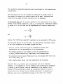
The evaluation of the physical inventory is a simple sum-up of product
batches weighted by a factor which indicates the fraction of the inventory material in each individual product batch according to equ.
=
time of introducing the step input signal
=
product batch size
=
weight fraction of the tracer
isotope in the two consecutive
superbatches 1) which form the
step signal
x.J.
=
weight fraction of the tracer
isotope in product batch i
1)"superbatch" is defined by a cer-t ai.n nu..nber cf input batches
with similar weight fraction of the tracer isotope.
(1
\
l'
I. I / •
-5-
The weieht factor of subsequent product batches illustrates the operator's
individual material management durine the passage of the signal throueh
the plant. Simulation studies and also experimental results indicate
that this factor converges to zero in a similar way as an exponential
function does.
The dispersion of the input step sineal can
be minimized if the operator runs the process according to a small number
of specified procedures,mainly by special operation of the headend and
product catch tanks but
only duringthe residence time cf the signal
in the plant.
This technique may also be applied when the use of three superbatches and,
consequently, two tracer isotopes is necessary. In this case the proper
formalism is more complicated (1), but its derivation does not need the
introduction of further basic concepts.
-62.
2.1
Technical Feasibility
MBA-System
Adefinition of "Material Balance Area" (lfMBA") is given in the basic
report of the lAEA INFCIRC/153
liMBA meana an area in
(a)
01"
/4/ in article 110:
outside of a facili ty such that:
the quantity 01' nuclear material in each transfer into or
out of each MBA can be determined;
(b )
end
the physical inventory of nuclear material in each MBA can be
determined when necessary, in accordance with specified
procedures,
in order that the material balance for Agency safeguards purposes can be
established" •
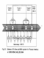
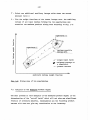
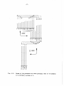
In connection with the application of the DPID the MBA has been defined
for two different plants.
The first one was the American
l~FS
plant, the
second one was the Belgian EUROCHEMIC where the method was very successful
in two integral experiments.
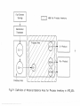
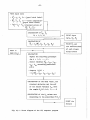
Fig. 2-1 shows the example of the NFS-MBA, Fig. 2-2 shows the EUROCHEMICexample.
In both cases the MBA system covered the process part only and excluded
the product storage araa because emphasis has to be laid on the condition
that the system response can be measured adequately. In addition it is
advisable to have only one significant input stream into the defined MBA.
IV
When the process needs auxiliary inputs of heavy material (e.g. the U
reducing agent in separation units) the DPID must be suitably corrected.
2.2
Design Limitations
In order to allow a fruitful application of the method a few limitations
should be kept in mind. They apply to the design and the operation of the
plant in question and to the material which is to be reprocessed.
Of
course there are interconnections between these parameters, e.g. it is
" Fuel Element
Storage
[
E>z=;=j
MBA for Process Inventory
'
[
Mechanical
Treatment
i
,
U - Product
I
--1
I
Pu - Product
Dissolver Area
Fig. 2-1: Definition of Material Balance Area for Process Inventory in NFS,USA
Produet
storage
Dissaver
MBA 12
I--
MBA 60
&0
-_.
I
/71
I
I
cn
I
Waste storage
I...-
Fig.2"·2
MBA 50
.
•
5c:heme of Pu-flow and MBA"·system for Process Inventory
in EUROCHEMIC, MOL,BELGIUM
evident that when large amounts of heavy material are mixed
the superbatches must also be large.
~n
big tanks
The limiting quantities for the superbatch sizes become smaller when the
mixing of material inside the plant is reduced.
As far as the design
is concerned, the following parameters must be taken into account:
a) The main influence on the dispersion or the step signals comes
from the mixing inside the tanks with a great hold-up of heavy
material, as buf'fer tanks, evaporators or product catch tanks.
b) A second contribution is due to the heels in the tanks which can be
inherent in the plant design or can be operation parameters.
The con-
dition of low heels - in order to have low mixing - should be mainly
respected during the passage of the step through the respective units.
c) Mixing inside the continuously working units of the plant (as mixersettIers) cannot be avoided without a washout. But since this mixing
is small, it can be left out. With the models which were constructed
in order to describe the flow of fissile material /5/ relatively good
correspondence of the theoretical and experimental results could be obtained, in spite of the fact that these units were neglected.
2.3
Operational Limitations
Generally speaking, the optimization of operations in a given plant with objective to allow the application of the DPID method must be solved case by
case
if there is only a limited quantity of material available. Simulation
studies, which use a proper model of the plant under consideration, or
historical experience
of operation can be of great help. The only general
rule is that the mixing should be maximized inside the superbatches and
minimized between two consecutive superbatches. It should be attempted
to homogenize the material inside the superbatches as much as possible.
The simulation studies of the Pu-cycle of the EUROCHEMIC plant - and
their results wbich were applied during the Mol III experiment - give some
hints on relevant operation parameters with respect to the influence cf
mixing. The studies were made on:
-10-
a) Residual heels in the head-end tanks.
b) Mixing procedures ln the feed tanks between the accountability
units and the first extraction cycle. This is possible
in
aplant with parallel intermediate storage tanks.
c) Recycles to the second purification cycle.
ad~)
rncreasing the
mi
xang in the he ad-rend tanks by enlarging the
heels can hell' to achieve a smoothing of the tracer concentration
within one
s~pe~batch+).
Obviously the prescription of minimum
heels at the step passage roust be kept.
Heels of 1
ad b)
%and
10
%were
studied.
Since the study of the mixing strategy in the feed adjustment tanks
of the first .extraction
cycle was connected with the variation of
other process parameters like the quantity of recycled material or
the number of batches taken into ac count for the calculation of the
concentration mean values for the superbatches, the results are not
completely clear. There seems to oe a tendency oy which the variance
of theroeasured inventory is lowered by the mixing strategy /5/.
ad
~
Reprocessing campaigns with (5 %) end without continuous Purecycling have been studied. The results show no significant
differences. The only important reroark concerns the magnitude
of the superbatches: a Pu recycle obviously increases the mixing
so that larger superbatches are needed in order to estimate the
process inventory with the same accuracy.
Two further important points are:
d) It has been shown in /6/ that the DPID method can also be applied successIV
.
...
fully ln
case of addltlonal
lnputs, as e.g. U -strearos.
'+ )This
strategy for the input accountability tank hasbeen calledexternal
mixing in
/5/.
-11-
It is possible to adjust the model for additional inputs either by
modification of the input or of the output signal.
e) A further operation requirement is to avoid batchwise recycling of
heavy material as far as possible.
2.4 Material Reguirements
It has been mentioned before that one of the most important conditions
for the application of the DPIDmethod is the availability of enough
material in each of the superbatches.
To give an estimate of the required
superbatch sizes one needs eitherpractical experience with the plant or a
rough model of the different mixing mechanisms.
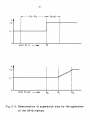
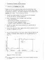
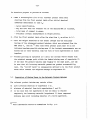
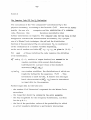
According to Fig. 2-3 it
can be deduced /5/ that for the case of two superbatches the first one should
not be smaller than Q2-Qo and the second one not smaller than Q2-Q1 •
Here Qo is the quantity of material which is produced up to the introduction
of the step, Q1 the quantity between the introduction of the step and the first
influence of the concentration c
in the product, and Q2 the quantity of material
2
which is produced up to the point where only material cf superbatch 2 comes out.
It is quite clear that the difference Q2-Q, gives the amount cf material
which is in a mixed state of superbatches 1 and 2. For the EUROCHIDUC plant
this &mount is about 3 times as large as the biggest heavy material hold-up
of any unit of the plant.
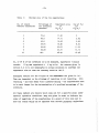
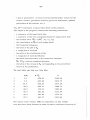
In order to get some more detailed information, simulation studies on the
EUROCHEMIC plant - under normal operation conditions, beginning with an empty
plant, and for a certain type of material - have been done in order to estimate
the amounts cf material in superbatches 1 and 2 which should be present for a
predetermined recovery of the inventory. The results are condensed in Table I:
-12-
.....
I
Q2- QO
I
C
c2-
I
.......
I
Q2- Q l ;
I
I
I
I
I
I
I
I
I
I
!
I
I
I
I
I
I
c,
i
I
I
i
i
I
0
i
total Pu in
I
I
I
I
I
i
I
I
I
..
l
i
1-
Q
x
. . . .-----+-----
O'--------------~---
total Pu out
Fig. 2- 3 ; Determination of superbatch s;ze tor the cpplicction
of the DPI D method.
-13-
Table I:
Minimum size of the two superbatches
No. of output
batches considered
4
70.6
86.9
5
6
96·9
99.44
99.90
99.98
100.
7
8
9
10
So, if 97
%of
Percentage of
the inventory
measured
Superbatch si ze
(kg of Pu)
10
(Q2-Qo )
11 0
(Q2-Q1)
11. 32
14.15
16.98
19.82
22.65
25.47
.28.30
0
2.83
5.66
8.50
11.34
14.15
16.98
the inventory is tobe measured,superbatch 1 should
contain
17 kg and superbatch 2 6 kg of Pu. FOT reasons given in
section 4.2 it is not meaningful in actual situation to increase the
superbatch size so that therecQvery wouldbe 100
%.
Analogous results for the U-cycle of the EUROCHEMIC are given in /3/.
They are dependent on the
stra~egy
of recycling or not recycling.
With
recycling - and that means with a greater mixing - the superbatches have
to be much larger for the determination of a prefixed percentage of the
inventory.
All these numbers are results which come out for a specific plant under
specific operation conditions. They are given in order to indicate the
order of magnitude of the superbatches in aplant cf this size and to
show the trends which can be expected with certain parameter variations.
-14-
3.
3.1
Generation of Adeguate Input Signal
Information Beguirements on Fuel Elements
The maximum benefit from the use of the illustrated teehnique is aehieved
when the physical inventory is measured with the lowest uncertainty.
A certain number of factors, which influence the statistical error of the
inventory, have been already indicated /7/. They concern essentially the
dissolution of the fuel elements available for reprocessing and the choice
of suitable procedures for the plant operations. This seeond group of
requirements
was
treated in 2.3.
The choices, which must be made apriori concern:
a) the isotope to be used as tracer,
b) the grouping of fuelelements in individual dissolution batches, and
c) the dissolution sequence of the batches.
It can be shown /6/ that the minimum
variance
,
er the Lnvent.orv
- is
achieved when the
minimum.
Here
c ....
i=:' ,2
~
where the sum is performed on j batches
of the i-th superbatch, c .. is the weight fraction of
~J
the tracer isotope in the j-th bateh of the i-th superbatch
M~. is the total mass of the heavy element inside one
~J
input bateh
-15Here the variances are
i
2
(J. = -_..:-.-:--~
LM .. (c .. -c.)
J ~J .~J
~
E .M7.
J
2
~J
1-
The expression
(J~+(J~
is an indicator of the batch to batch variation in the
weight fraction of the tracer
isotope~
and
/c,-c 2' is the step size.
As
long as every isotope of fissile material (of Pu or of U) may be
used as
tracer~
a suitable analysis of the material to be reprocessed
must be performed. For this reason the following information must be available for proper treatment:
- The number of fuel elements to be reprocessed, divided according
to the type of reactor and of initial
enrichments~if they
differ.
- The number of fuel elements of each type, that are dissolved together
asa "s ing.le " batch ,
- Final quant i ties of Pu and U, contained in each fuel element (or
asseIJl.bly) and their isotopic composition ~as calculated by the
reactor operator.
The above mentioned data are usually communicated as shipper dnta by
the reactor operators to the reprocessing plant management and, for
power reactors, it seerns that thera is no reason for their classification.
On the basis of these data the batches will be constructed and ordered.
In those cases where the results of input analysis show that another
tracer is more suitable the tracer
on a priori basis.
CAD
be different from the one chosen
-16-
3.2
The Determination of '.'Super Batches"
When our method of inventory determination is used, the first constraint
of "sufficient quantity" of material +) must be satisfied. In prac:tice
two cases are possib1e:
a) The step in the weight fraction of the tracer isotope will take p1ace
between the reprocessing of two
different~es
of reactor ruels.
b) The step will be created by suitable selection and ordering of the
fue1 elements of one reactor.
The two cases are conceptual1y not different, but, in practice, it is
better to follow two different approaches. In both of them it will be
possib1e toprofit from the use of a computer
cod~
i11ustrated in Annex 1.
It is necessary to stress that the optimization procedure, that will be
described in the following pages, allows the optimal sequence determination
for the measurement of the Pu or U inventory.
that the best input
sequenc~e
Nevertheless it i6 possible
for one of the elements (Pu, e.g.) is apt to
generate a "step" useful for the other element inventory. This second "step",
however, is not necessari1y optimal.
Let us assume that a Pu inventory measurement is required. In the first case a},
we have the fo11owing problem: There are N fue1 elements (of equal. type),
..
4 .
•
that must be used to create a superbatch, cDntaining at least a prescribed
quanti ty of Pu. In other words, the minimum number of batches n , which are
necessary to create a superbatch of the prescribed quantity Q, can be ca1culated as fo110'W's:
n
=J
O
(-JL)
mq
In this formula the fo11owing quantities are given:
n
:=
Q ==
m
=
q
:=
number of batches for the constructlon of a superbatch
quantity of Pu insidethis superbatch
number cf fue1 elements in one batch
mean quantity of Pu in cne element (the computer code haB been written
for equa1 amounts of Pu in all the elements, see below)
+) see section 2.4.
-17-
is a function that defines the minimum integer number with Q/mq
as the argument.
j
The "sufficient quantity" constraint can be expressed as
The computer code given in Annex 1 has been written with the constraint
that the aaourrts of Pu (and U) in all the elements are equal. Nevertheless,
in many actual cases, the mass differences of different elements are not so
large to render relevant changes in the results.
It must be recalled that
the batch construction' is made on the basis of reactor data which can be
affected by not negligible errors: for this reason, in most cases, a more
sophisticated analysis 6n such data is useless.
The n batches must be constructed in such a way that the batch to batch
variation of the tracer isotope is minimal.
This operation must be performed
on all of the Pu (U) isotopes in order to select the tracer isotope. This
tedious exercise is automatically performed by the GROUP code (Appendix 1).
Fo~
each Pu (and U) isotope the computer code gives:
- the list (if
~~y,
when N n) of the N-n elements not considered,
- the optimum grouping of the elements in n batches of each containing
m fuel elements,
- the expected relative weight fractions of each isotope in each bateh,
and
- their expected mean values and variances for the superbateh.
(The latter may be interpreted as a measure of the batch to batch
variation. )
When more than n batches can be constructed with the N elements it is suggested
to run the code for superbatches composed also of n+1, n+2, .••• batches.
In fact it is possible that no significant change
~n
c (mean value of the
tracer weight fraction) and no increase in its variance occur. In this case
the use of a larger superbatch is advised, because this guarantees that the
"sufficient quantity" constraint is better satisfied.
-18-
The calculation described heretofore must be performed for both superbatches
independently.
When the results for &11 the isotopes are available the proper choice of
the optimal Pu isotope to be used as tracer can be made.
Obviously that
tracer will be chosen for which the ratio (3.1) is minimized.
In the second case, b), the problem consists in the construction of two superbat ches , with minimum quantities Q1 and ~, by putting the N available elements
in groupe of m. In this ease the two superbatches will consist respectively
of
n
=j
1
Q
(..J.)
mq
and
batches. The "sufficient quantity" constraint can be expressed as N::'(n 1+n2)m.
The following results for each Pu and U are obtained when the proper values
of the input parameters of the GROUP program are used ,
- the list (if any, when N>(n 1+n
of theelements nottaken into
2)m)
consideration for the determination of the superbatches,
- the optimum grouping of the elements in the two superbatches of
n 1 and n
2
batches respectively, containing m fuel elements each,
- the expected relative weight fractions of all the isotopes (for both U and
Pu) in each bateh, end
- their expected mean values (for each superbat.eh ) and variences.
When more than n
1+n 2
batches may be constructed with the N available
elements, it is suggested to TUn the computer code increasing the parameters
n 1 and/or n 2 and to decide, from the examination of the results, if an
increase in the quantities Q1 andlor Q2 is possible. However, it must be
recalled that this increase of the "minimum quantities" is possible and
advisable only whenno significant increase of the ratio (3.1) occurs.
-19-
3.3
The Determination of the Input Sequence
The problems concerning the tracer isotope selection end the composition
of the single dissolution batches have been solved. The last decision,
that roust be taken before the dissolution,is the determination of the input
sequence for the batches of the two superbatches.
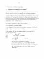
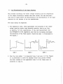
Two rules should be respected:
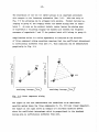
1. The regression lines, which approximate the histogram of the tracer
weight fraction versus total material quantity, must be as flat
as possible for both superbatches. !t has been demonstrated that
any divergence of the regression line trom the horizontal decreases
the precision of the final result. (Avoid the case 1, illustrated in
the figure • )
I
I
~
1~
I
I
I~
r~-
CASE 1
CASE 2
CASE 3
2. When the rule number 1 is respected (case 2 and case 3 of the figure)
it is preferable to shirt the maximum tracer oscillations towards
the first batches of the superbatch (case 3 of the figure must be
preferred to case 2).
-20-
3.4 Practical Problems
Sometimes it happens that the required grouping or elements ror the
construction or the dirrerent batches and/ or the prescribed input
sequence can not be rulrilled because of handling difficulties inherent to the storage location of the reprocessing plant. In such
cases the inventory taking should be planned sufficiently early, to
solve the problems indicated at 3.2 and 3.3 before the fuel element
shipment. In this case the shipment and the storage may be, in time,
planned in such a way that the handling difficulties at the reprocessing
storage pond are overcome.
4.
-21Procedures to Determine Process Inventory
4. 1 Analysis of the Measured Input Signal
Because of thelack of adequate shipper data the realized input step
signal may show considerable differences from the provided input signal
as specified in section 3.
measured input signal.
All furt her evaluations 'Will be based on the
Thus we proceed as follows:
A - Specif'y the nuclear ma.terial (U or Pu) which is to be balanced
by book and physical inventory comparison.
B - Make a chronological list of relevant input batch data:
- batch identification,
- date and hour of transfer (as specified in 5.1),
- total mass of element expressed in grams,
available isotopic measurements in weight percent.
C - Specif'y thesingle input batches forming the two superbatches as
given in section 3.
D - Select that particular tracer isotope which shows the smallest ratio r
•
•
as g1ven
kn
.
•
equat~ons
(~1
~ ~,+) •
\J' '-J'JI
E - Plot the weight fraction cf the tracer isotope versus the mass of the
element ot: subsequent input batches for the two superbatches as in
Fig. 5-1:
i :
--IM.. i_-I
I lJ!
-,I
_ _ _._---i-
maas of
."........
element
Fig. 5-1: Isotopic input signal
+} r .
gives alreaUy a first estimate of the relative standard deviation
ffiln of DPID
-22-
F - Select one additional auxiliary isotope which shows the second
smallest ratio r.
G - Plot the weight fractions of the tracer isotope vers. the &uXiliary
isotope of all input batches forming the two superbatches and
establish the maximum possible mixing area according to Fig. 5-2.
superbatch II
o - single input batch
"
- weighted average of'
a superbatch
+ - product batches
auxiliary isotope weight fraction
...
Fig. 5-2: Mixing area of two superbatches
4.2
Analysis of the Measured Product Signal
The main problem in this analysis of the measured product signal is the
determination cf the "cut-off bateh" whieh will not show any significant
fraction cf inventory material. Consequently all the following product
batches will also not give any contribution to the inventory.
-23-
We therefore propose to proceed as follows:
A - Make a chronological list of all relevant product batch data
starting from the first product batch after initial physical
inventory measurement at time t :
o
-batch identification,
day and hOUT when the transfer out of the defined MBA is finished,
- total mass of element in grams,
available isotopicmeasurements in weight percent.
B
Find the first product batch after the step time t
1
as given in 5.1.
C - Plot the weight fractions of the tracer isotope and the auxiliary
isotope of the subsequent product batches, which are released from the
MBA after t 1 (see B).+) Note that every product point must be in the
indicated maximum possible mixing area if the isotopic measurements are unbiased and no other material than the fuel of both superbatches is mixed
together.
D - Proceed plotting as specified in C until the isotope veotor merges with
the weighted average point within the dashed mixing area of superbatch H.
If the next few product ba.tches COllie roughly to the same point, one can
be sure that all inventory material passed the product accountability
tank.
The llcut-off batch" is consequently defined to be tbe first product
batch which reaches the weighted average of superbatch II.
4.3 Separation of Mixing Types in the Relevant Product Batches
The relevant product batches may contain either
a)
pure inventory material of superbatch I
b)
mixtures of material from both superbatches I and II ..
c)
In the case that the superbatch
01',
Ir was teo small to replace
completelythe inventory material (superbatch I) three component
mixtures may occur including material of a third superbateh.
+) This information should be summarized in Fig. 5-2.
-24-
The separation of the two (or three) groups is an important procedure
with respeet to the inventory evaluation (Sec. 4.4).
With the help of
Fig. 5-2 the grouping can be arranged very quiekly.
Produet batehes be-
longing to group a) are roughly within the dashed mixing area of superbateh I.
As soon as the produet isotpic vector leaves the mixing area
of superbateh I following roughly the dashed line between the weighted
averages of superbatch I and II the produet bateh will belong to group b},
Complications arise if a third superbateh is involved as the solution
of three component mixing equations requires that the coefficient determinant
is suffieiently different from zero /1/. This condition can be demonstrated
graphically in Fig. 5-3.
II
1-,
!.......1
0
-
Irr
,):
'-l
II
Cl)
Pt
0
~
/
0
lIJ
-r-!
J...
Cl)
u
lIlI
J...
+'
I
/
/
~
/
S
0
I):
-.....j
/
Cl)
g.
+'
0
lIJ
-r-!
III
J...
9
Cl)
u
lIlI
J...
+'
Fig. 5-3: Three component mixing
The figure on the left demonstrates the conditions of an unsolvable
equation system where the three components (I, 11, 111) are linear dependent.
The figure on the right shows an example of a solvable equation system
where the eoefficient determinant which is proportional to the shadowed
mixing area is sufficiently different from zero.
-25-
It is recommended to avoid the three component mixing system by
the size
o~
superbatch II.
Only
~or
enlarging
reasons of completeness the relevant
procedures for the evaluation of the inventory including a three component
mixture is also outlined in the following section. Product batches which
contain components of three superbatches can be identified by plotting
the corresponding isotopic data in Fig. 5-3.
In case of a solvable equation
system (figure on the right) the product point is located clearly within the
maximum possible mixing area.
4.4 Evaluationof the Physical Inventorr
From the analysis of the measured input signal (Sec. 4.1) it is possible
to perform the final choice of the tracer isotope (or isotopes, when three
superbatches must be considered).
The analysis of the output signal allow the separation or the output batches
in two (or three) groups, according to their content (Sec. 4.2 and 4.3).
The results of the previous analysis allow a simplification in the determination of the inventory. In fact the inventory value, H, may be expressed as
( 4.1)
where Hi is the contribution to the total inventory of the i-th group.
In the following each single contribution will be evaluated independently.
In 4.4.4 the evaluation of the whole inventory and
will be outlined.
its statistical error
-26-
4.4.'
H, Evaluation
The eontribution of the first group of batehes to the inventory is simply
given by
n,
(4.2)
H,
= 1:.,J. M.oJ.
•
•
0
where n, J.S the number of batehes of the fJ.rst group and Mi are the masses
of heavy material (of the first superbateh only) present in the i-th output
bat eh.
The eontribution H, is independent of the evalues (weight fractions of
tracer isotope), so that the statistieal error of H, may be easily ealeulated
from the errors of the single mass m.easurements. These errors are usually
small (=
<,%) and normally distributed. Thus, it follows that
n,
(4.3)
2
°H 1
H
2
20
= 1:1J..
'OM
_
Evaluation
The definition of H
2
is given (see ,.,) by
n
(4.4)
J.
H
2
x.-c
2
= 1:., J.
M?
1.
2
...::J._::.
c.-c",
,
t::
n being the number of batches of the second group. All the other symbols
2
have been already defined.
The use of the weighted average concentrations c 1 and c may have a biased
2
estimate of H +). Due to the fact that the theory is still not sufficiently
2
developed to indicate how to calculate these values in order to obtain a
better estimate cf H the following approach may oe used.
2,
+)L. Farese - private communication.
-27,.0
Let us assume that the independent variables Mi'
xi' c 1, and c 2, are real'~zat·~ons
of random variables each of which has a known prescribed pdf (probability
density runctd on}, For the values M~ and x. the pdf' s are assumed to be normal
~
~
with mean values equal to the measured ones and standard deviations equal to
the standard errors
of the related measurements.
The variables c'1 and c'2 are given by
i
rkMk·I\:·c
J
J k J·
(4.5)
c~ =
i
J
rkMkjI\j
j
::
1,2
where the sums are performed on all the input batches of the j-th superbatch
and where
~j
~s
the input mass of the heavy material contained in the
k-th batch of the j-th superbatch,
ckj
is the weight fraction of the tracer isotope in the same
baten end
R
are random numbers extracted from a (0,1) interval with
kj
~~iform
distribution.
2
Consequently, ci end c are also random variables, end their mean
values end standard deviation m!o/ be calculated. Note that the previous
formula assures that Ec!
J
= c.;
J
and that
min (c .) < c! <. max (c k.)
kJ - J J
(4.6)
The repeated use of the formula
•
•
L4.4_1 for
a high number of realizations
0
of the andependerrt var1.ables M., x, , c ! allows the computation of a high
~
1.
J
number of contributions of type H related to the real input signal. It J.S
2,
then possible to calculate the frequency curve, the distribution, the meen
value end the variance of the reRlizations cf H The frequency curve may
2•
be interpreted as the probability density function of H2, so that it is
possible to determine its expectation value and the error limits, according
to a prescribed confidence interval.
These operations may be easily effectuated by a computer, employing the computer
code CC2, described in Annex 2.
-284.4.3
H Evaluation
3
The DPID requires sometimes the use of a "three component" system (three
subsequent input superbatches, with two selected isotope tracers). In this
case a further contribution to the inventory is given by
(4.7)
where the sum
1S
performed over the
"s
batches of the third group and where
1
(4.8)
T.
:=
1.
x.1.
°2
s,1.
d
1
1
c1
c
d.I
d
2
c
d
3
3
and
(4.9)
D
==
2
2
c
3
d3 I
c j end d j (j == 1,2,3) are the concentrations of two tracers (e.g. Pu-241
and Pu-242) in the j-th input superbateh. x. and y. ar'e the concentrations
1.
1.
of the same isotopes in the i-th output batch.
The inadequancy of this theory in respect to the treatment of real cases
results from the same reasons pointed out in the case of the "two component"
systems. It follows that the evaluation of the experimental data ~ be obtained following a procedure similar to the one outlined in the previous
paragraph.
In this case, however, it is necessary to pay some attention to the fact
that the selection of r-andom values for the pairs c ~, d ~ must respect the
J
J
physical correlation existing between these parameters. The use of the
following system
1.
(4.10)
c~
J
'"
LkMkjRkj ck j
i
IkMkjI\j
j == 1,2,3
(4.11)
i
rkMk'I\'~
J J J.
d~ ==
i
J
l:kMkjI\.j
-29-
lcgically justified by the equation
L-4.5J
(the symbols have the same
meaning) indicates that single values of c! and d! are obtained as randomly
J
J
weighted means of the concentrations of the input batches c. and d .• It follows
J.
J.
that, in every realization of the pair of random variables c!, d!, the same
J
J
contribution of the individual input batches to the means must be considered.
The use of the same weighting factors (~j ~j) in both equations of the
system assures that the physical correlation existing between c and d inside
each single superbatch is respected.
Siroilarly to the previous oase of H the contribution H is evaluated many
2,
3
times as function of independent variables randomly selected from the mentioned
distributions. The analysis of the results of this application of the Monte Carlo
technique gives the expectation value of H its pdf, and the error limits,
3,
according to a prescribed confidence interval.
These calculations may easily be effectuated by a computer, using the computer
code CC3, described in Annex 3.
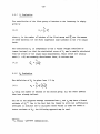
4.4.4 Total Inventory Determination and Error Limit Estimation
In the previous sections it has been indicated how to calculate the different
contributions to the total process inventory and how to interpret each cf them.
=
The pdf's that have been associated to the measurement of each H1( 1
1,2,3}
represent the confidence, that can be attributed to the measured figure. When
a variable is normally distributed, its pdf is simply specified by the value
of the standard deviation parameter. This is the reason that 10 or 20
values
are orten used when ccnfidence intervals are given. The approximation cf the
pdf of H and H with anormal runction is, generally, not valid. Therefore
2
3
a more sophisticated error propagation analysis is given below.
Finally the pdf roust be calculated for the whole inventory H. This will give
an immediate picture of the measurement significance.
This kind of pdf is
obtained by subsequent convolutions of the pdf's of the addends H1, H2 and H3•
The definition cf these convoluticns is given in Appendix 4. For the moment,
however, it is sufficient to remember that in this case the pdf's are given
in form. of histograms and that the convolutions reduce to simple sums. The
pertinent formulae are also given in Appendix 4.
-30-
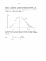
However~
it is important to stress the physical significance of the
formalism connected with the pdf of the quantity R. In the figure an
example cf such a type cf function: h(R} is plotted. The area under
the curve is, by definition, equal to 1.
!
J-l
_I
!
h(R)
_1
-1-c~i------_.---+-,-~_. _.,,~~. ~H-
q
H + ~
H
1
H
As expectation value the mean value .H i8 choosen. The error limits
connected with a prescribed ccnfidence p are the values H-q l and H+q2'
such that:
R
J
H-q
h(H}dH
1
= p/2
fH+q2
h(H)dh
==
R
-31-
5.
Book Inventory Determination Procedures
5.1
Definition of the Time Interval
The physical inventory determined by DPID (section 4) represents the inventory situation vithin the defined MBA at the time (tl) vhen the isotopic
step signal is introduced.
As this time (tl) i5 very important for closing the material balance, more
specifications must be given:
- Case I: The input accountability tank (IAT) is located outside the defined
MBA-system.
The relevant time point is defined at the beginning of the
transfer of the first input batch of the second superbatch from the IAT to
the next process unit.
- Csse II: The IAT is located inside the defined MBA which is sometimes so
the case that the adequate shipper-receiver differences
C~~
be eatablished.
The relevant time point is defined at the beginning of the transfer of the
first input batch of the second superbatch from the dissolver tank to the IAT.
In the case that there are relatively great heels in the IAT one has to
relate the isotpic signal to the incoming material end not to outgoing
material as it is done in csse I.
Correspondingly the book inventory (B), vhich is to be compared vith the
physical inventory (H) (determined according to the procedures specified
in section 4),has to be related to the time point defined above.
5.2
Evaluation of Book Inventory
The evaluation of the book inventory is a weIl knovn procedure vhich needs
not to be specified in detail here. The relevant equation is given belov:
-32-
where
beginning inventory at time t
BI(t)
o
I,P,W
:=
i,p,w
o
input, product and waste batches
number of input, product and wa.ste batches
between t o and step time t,(as defined in section 5.')
The input accountability stops with the last bateh of the first superbatch.
However, only those product and waste batches are accounted for,which
are completely transfered out of the defined MBA between t
o
and t,.
5.3 Determina.tion of the Variance of Book Invento;y
The Rela.tive Standard Deviation (RSD) associated with each fIo'W can be calculate.d vith
ö2
r)
n
volume,
weight
+
(RSD)2
where
Ö
B
calibration error
Ö
:=
precision cf the measurement
c
r
=
=
n
m
1
RSD
number of batches
number of analyses per batcn
Equ. (5.2) i8 valid if all the batches have equal volumes (weights) and
concentrations. This assumption appears to be justified.
C&1ibration error
and precision have to be estimated fram the experience of quslity control
procedures.
The resulting variance of the book inventory is the sum of &11 the variances:
a2
B
=k
2
2
ö ·(~F) ; F := I, P, W, BI
F F
-33-
6.
Procedures to Determine the MUF
6.1
Book-Ppysical Inventory Difference
From the point of view of the safeguards control the main interest of
the DPID i8 the comparison between the measured value (H) end the accountability value (B), usually referred to as book inventory.
The difference between these two quantities is the weIl known MUF
(Material Unaccounted For), defined as
(6.1)
MUF
=B -
H
The calculation of such a quantity and of its statistical errors is of
capital importance for the control activities. In fact the article 30 of
INFCIRC/153 /4/
explicitly requires a statement on "the amount of material
unaccounted for over a specific period, giving the limits of accuracy of
t he amount a stated".
6.2
Confidence Intervals
As illustrated in 4.4.4, the determination of the limits of accuracy fqr the
MUF is deduced from its pdf. Such a function i8 obtained, asin the case
of
the whole inventory, by a suitable convolution between the pdr.s
associated to R end B. The first has been calculated in 4.4.4; the second
is simply a normal distribution, the mean value and standard deviation of
which have been deduced insect.5.rndicating by heR) and b(B) such pdf.s,
the pdf for the MUF, m(MUF) is given by
~
(6.2 )
m(MUF)
=1 b
(MUF+x) • h(X) dx
J
or by a suitable approximation of this
integral with a sumo
This operation is described in more detail in Appendix 4, where the performances of a computer code ,vhich may be used for cal.cul.et i ona , ar'e
illustrated.
6.3 The "Statement" on the MUF
In
theory~
if a facility has a perfect accountancy system for all the in-
puts Md outputs, the MUF should be only the consequence of cumulated
measurement errors. Its va.lue, if not zero, should be "consistent" with
zero. The analysis of the MUr measurements must then state a conclusion
about such "consistency".
The determination of the required statement is straight forward when
the error distribution (the pdf) areund the MUF (the mean value er
such a distribution) i5 given.
Let p be the value fixed apriori of the probability level requested for
the statement +). With the employment of the same technique reported in
4.4.4 it is possible to define the two error limits m1 and m2 for the
measured value of
MüF.
Two cases must ce considered
(a)
HUF
MUF - m >0
1
In the case (a.) it is possible to state that the measured MUF is "consistent"
with 0 (with a conf'Ldence p); in the case (b ) the measured MUF is "not consistent" with 0 (with a conftidenee p).
A third case is theoretically possible: MUF + m2 < o. This last case , in
spite of' the fact that it gives a piece of' information on the "sare side"
from the safeguards point of view, should impose deeper investigation on
the process accountancy techniques (measurement included)
01"
on hidden
inventories inside the process area.
+)The "working group meeting on quantitative data and results of
systems analysis and integral tests" (Vienna 4;" 8.10.71) suggested
values of p in the range .90 T .99; usually 95 %is adapted.
-35-
In the case (a) mentioned before it is possible to calculate the
probability that the MUF is equal or lover than O. Such value is simply
(6.3)
p(MUF<O)
= Jr
o
m(MUF) d(MUF)
This is a further information, that quantifies the agreement between
B and H at the moment of closing the balance.
Another interesting statement, from the point of view of the safeguards
control, concerns the comparison of the measured
~IF
with a threshold
amount (e.g. the LOA referred to in ref. / 8/). Such a statement is
obtained in the identical
w~
in which the provious has been obtained.
It is sufficient only to substitute the 0 by the actual value cf the
threshold.
Acknowledgement
The authors are grateful for the help cf Nebojsa Nakicenovic who has
reviewed the manuscript.
-36-
7.
/1/
Literature
H. Winter et al.
Determination of In-Process Inventory in a Reprocessing
Plant by Means of Isotope Analysis.
KFK 904
July 1969
/2/ R. Kraemer, W. Gmelin et a1.
Integral Safeguards Exercises in a Fabricating and a Reprocessing
Plant.
IAEA SM-133/86
/3/
1970
R. Kraemer, W. Beyrich et al.
Joint Integral Safeguard Experiment (JEX 70) at the EUROCHEMIC
Reprocessing Plant, Mol, Be1gium.
KFK 1100, EUR 4576e, 1970/71
/4/
lAEA
The Structure and Content of Agreements between the Agency and
I
the States required in Connection with the Treaty on the NonProliferation cf Nuclear Weapcns.
INFCIRC/153
/5/
M~
1971
E. Drosselmeyer, R. Kra.emer, A. Rota.
App1ication of Digital Simulation Techniques for Process
Inventory Estimätion.
lAEA SM-133/18
1970
/6/ Rer. (3) Chapter 4
/7/
Rer. (3) Chapter 5
/8/ W. Gmelin et
al.
A Technica1 Basis for International Safeguards.
A/CONF.49/PI773
Ju1y 1971
-37-
Annexes
In the following pages a short description of the computer
code s ,
suitable for data handling of the DPID, is g iveri,
The listings of such code s , written in FORTRAN language, may
be found, together with the solution of sample problems, in the
external report EUR
4833.e
Dynamic Process Invento rje
: "Four Computer Codes for the
Determination - Application in
Safe gua.r ds " by A. Rota (1972).
-38-
Annex 1
The Computer Code GROUP
The computer code GROUP
has been designed to provide the
information necessary for the composition of the single input
batehe s , when a DPID is pfanne d,
The problem hasbeen outlined in paragraphs 3. I and 3.2.
The input data which define the problem are:
the tota.l nearnbe r , N, of the available fuel elements (of the
same reactor and approximatively of the sarne enrichment);
the number of e Iern.ent s , rn, of which an input batch is
composed;
the total number of batches desired in superbatch 1 and superbatch 2 (NI a nd N 2 respectively);
the narne of each fuel element available for reprocessing together
with the calculated values of its content in Pu and U isotopes.
When both NI and N 2 are different from z e r o , the code defines the
optimum grouping for the construction of two superbatches. When
either NI or N2
NI
=0
is zero,only one superbatch is constructed. If
the superbatch is constructed in such a way that the higher
tracerconcentration is selected. When N 2 = 0 the minimum tracer
concentration is selected.
Note that when both NI and N
are different from zero, the first
Z
superbatch will be constructed with the minimum tracer concentration
and the second with the rnaxi.mum one , When a going down "step" is
des i r e d; the two superbatches selected by the code will be used in
inverse o r de r ,
The selection of the g r oupi.ng of tbe element for ea ch bateh of the
required superbatches is made for each isotope, both of U and Pu,
present in the burned fuel elements. For each of these isotopes,
and according the specifications required (NI' N2' NJ, the GBOUP
code gives:
-39-
the list of the elements not utilized (when (N 1 + N Z) • rn c N),
the list of the groups of fuel elernents, which constitute a
b at ch ,
for e ver'y constructed batch the expected abundance of ea ch
Pu and U isotope,
for every superbatch the mean values and the standard
deviations of such .abundances ,
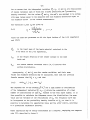
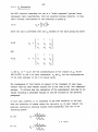
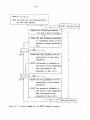
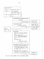
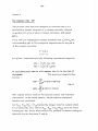
The block diagram of thecode i s reported in fig. A1-1.
Fig. A1-2 shows an. example of batch grouping for a case of
12 elements which are to be divided in groups of 3.
-40-
READ N, N
N
m
l, 2,
READ The name and the characteristics
of each fuel element
I
L,
---------;
PRINT the input data
I
I--
t
I
I
ORDER the fuel elements according
to increasing values of the
I
selected isotope concentra=
tion
no
I
yes
I
SELECT the m.N1 elements for the
construction of the first
I~
I
superbatch
SELECT the groups of elements of
each batch of the superbatch
I
I
(see the s cheme of the
procedure in Hg. Al-2)
N
2
yes
=0
..
no
? I-~.;p.;;.-----
SELECT the m.N
2
elements for the
construction of the second
superbatch
SELECT the groups of elements of
each batch of the superbatch
(see the scheme of the
procedure in fig. Al-2)
:
Fig. A1-1:
Block diagram of' the GROUP computer progrm
PRINT the results
-41-
f
f1r-··f#f4hl
1 2 345 6 7 8 9
t
jl
~
==
t:::::t
11 ·12
\
")
\
1
STEP ..
5 6 7 8 10 12 9 11
._---~..;!.........,yt}JJ ~
frr ,i
n
STEP
5 6 7 8
2 912 10
11 4 t 3
Fig. A1-2:
Schemeor the procedure ror batch grouping: Case of 12 elements
to be divided in grOu.-Pii cf 3.
-42-
Annex Z
The Computer Code CC2 for H Evaluation"
2
The calculation of the "two component" contribution HZ to the
physical inventory, according to the formula (4.4)
jus tify
the use of a
code , However, this
does not in itself
computer and the construction of a computer
becomes unavoidable when
further information is r equi r ed, Thecomputer code CC2 has been in fact
designed to calculate the measurement uncertainty. By a proper
use of a Monte Carlo technique, the pdf and the distribution
function of the parameter HZ are calculated. HZ i s considered
as the realization of a random variable depending,
on the set of random variables Mf, xi' c1' cz, as given in (4.4).
For
each
of these variables the co de requires the definition
of its distribution.
Mf arid xi (i
= 1,
nurnbe r of output batches) a r e assumed to be
r andom variables with normal distributions
individuated by a proper value of the standard
deviations
Cl and Cz
«(5Mi ' erxi)
are random variables, the distributions of which are
implicitly defined by the equations
(4.5)
. This
formalism i s used by ccz. 1t follows that the input
batch characteristics
(M~j'
Ckj) must be introduced
a s input data for the program.
Further input data for the CCZ are:
the number N of "ht stor-Ie s " requested for the Monte Carlo
procedure;
the range that should be covered by the error analysis;
the step magnitude for the frequency di st.ributfon, and then
for the p. d. f , ;
the list of the particular values of the probability for which
an error boundary definition i s particulary interesting;
-43-
a list of par arrie.te r s
of rrririo r intarest (initialization values for the
random nurnb e r 'geneJration r outine s , print-out definitions, optional
perforation ci t.he r e sult s , etc , ),
Fig. A2-1 reproduces a logical flow- sheet of the program.
The output of the programcontains the following information
a summary of the input batch data
a summary of the "two component mixture" output batch data
the median value HZ
=f
(M
f , xi,
C 1, CZ)
the contribution to HZ of ea ch output batch
the frequency histogram
the table of the pdf of HZ
a rough plot of such pdf
the table of the distribution of HZ
a rough plot of such distribution
the rna i n cha r a ct e r i s ti c s of th e s ta.ti s ti cal ana.ly si s r
HZ, G'"HZ' relative standard deviation
the table of the values of HZ corresponding to th e prescribed
values of the pr ob ability .
The last table can look e.g. like this:
P(X)
X- H2
X
I
2.5
-5Z8.93
Z 3Z0. 94
2
5.0
-433.08
2416.79
3
10.0
-332.67
2517.20
4
20.0
-209. 17
2640. 70
5
80.0
179.53
3029.40
6
90.0
261. 62
3 111. 49
7
95.0
3Z1. 26
3171.13
8
97.5
365.57
3215.44
The values of the column P(X) are input data , In this samp1e
case they have been choosen in order to select confi deric e i nt e r va.l s of
-44-
95
% ) 90 %,
80
%,
60
%;
in fact the error limits for a 95
confidence are located at P(X)
H2 = H2
= 2.5
%
(%) and 97.5 (%); this gives
+365.57
-528.93
The sarne procedure is used for the other confidence intervals •
-45-
READ INPUl' DATA
- ~,
J
-
0
M. ,
~
c.
( j = i.nput batch index )
x.~
( i
J
= "Two components"
~utput
-
°M~~
0
~
x.~
batch index )
o
(standard errors of M.)
~
~
and x.)
~
CALCULATION of the weighted values
cl
C2
and
PRINT input
I
CALCULATIONof H
2
= f2(M~,
=
xi'
PRINT
and
2
the contributions
cl' c2 )
H
of each single
READ
N
READ
POL)
j ourput bateh
"--_
_---..JI
~
CALCULATION
Repeat the following procedure
for k
= 1,
2, ••• N :
o
• Select randomly Mi k, x i k ' c lk '
and e
according prescribed
2k
pdf
• Calculate H (k )
2
=
=
f2(~k;Xik,c1k,c2k)
CALCULATION of the mean value, the
standard deviation and the pdf
of the random variable H , from
2
the sample H (k), k=l, 2, ••••• N
2
CALCULATION of the H values cor=
2
responding to the prescribed P(X.)
~
PRINT the
re sul.t s
Fig. A2-1: Block diagram of the CC2 computer program
-46-
Annex 3
The Computer Code CC3 for H Evaluation
3
The code CC3 evaluatesi. the "thr e e cornponerrt" contribution,
H3, to the physical inventory. Is is conceived and constructed
identically to the CC2 (Annex 2). The only obvious differences
concern the formula for the H3 calcu1ation (4.7) and the system (4.10,
4.11)
which defines the distributions of the r andorn variables
c. and d., , j
J
J
= 1,
2, 3 •
Fig.A3- 1 illustrates the logica1 flow sheet of the program.
The list of the input requirements and of the output results is
identica1 to thatillustrated for the code CC2. In this ca s e ,
obviously, the input batch characteristics must inc1ude 3 superbatches (j
= 1,
2, 3) and two weight percent ages of tracer Laot.opes ,
In particular, the program needs:
i
M. k' c· k' d. k
J'
J
J,
where k is the index of the k-thbatch of the superbatch j.
-47-
READ input data
i
= ..!.nput batch Index)
(j = "three components" ~utput batch Lndex)
- M , c , d (n
n
n
n
-:-:0
-M.,
J
-
x.,
-
y.
J
o
- O'M , O'x.'
J
J
J
"s,J
(standard errors of
~_
_
x.,
M.,
J
J
y.)
J
CALCULATION of ~,
(h
L...-
= 1,
dh
2, 3)
---
--'
PRINT input
da'ta ,
I
eh' ~
CALCULAT ION OF
H3
= f 3(Mj, Xj ,
Yj' ~,
dh )
I---
PRINT H and
3
the contributions
of each single
READ
N
output batch
READ P( X. )
~
CALCULATION
Repeat the following procedure
for k
= 1,
2,
0 0
•
0
N :
• Select randomly M;k' x j k ' Yjk'
c
d
accordäng prescribed
hk' hk
pdfos·
o
Compute H
=
3(k)
o
= f 3 (M j k, x j k' Yjk " c hk' dhk)
CALCULATION of the mean va.lue , the
s tandar-d deviation and the pdf
of the randorn variable H
frorn
3,
the sample H
k=l,
oN
3€k),
2'00.0
cALCULATION of the H val.ues cor=
3
responding to the prescribed P( Xi)
PRINT the
results
Fig. A3-1: Block diagram of the CC3 computer program
-48-
Annex 4
The Computer Code
MUF
The present code has been designed to calculate the p. d , f.
(probability density function) of a randorn variable, defined
a s analgebraic surn of others randorn variables. with known
pdf.s.
Let p arid q be independent randorn variable sand f 1 and f
2
the
corresponding pdf , s , The analytical expressions for the pdf, s
of
~he
randorn variables
s
= p+ q
r
=p -
q
are given, r e spective ly, by the following convolution integrals:
g{s)
her)
= jf l [t}, f 2(s-t)dt
=!f l(r+t).f2(t)dt
In this particular aase we will express the f.s in the form o~
histograms.
. The previous integrals then
becorne :
K2
G(S)
=L K (F 1(K).F2(S-K))
Kl
J2
(A4.1)
i
H(R) = 2: li' l(R -J)- F2(J))
Jl
(The capital letters used for the function narnes and variables
correspond
to the srnall letters, which indicate continuous
function and variables).
Let N 11' N 12 (N 11
< N 12)
define the integer interval outside which
Fl i s identically z e r o and let N
N
(N
have the same
2 1,
22
2 1<N2 2)
rneaning for F2. From these limits it is po s s.ibl.e to deduce analogous
intervals for the functions G and H:
Ignoring those terms which certainly do not give any contribution to
the sums (A4.1), the sum limits become:
Kl = Max (N 11' S-N
K2 = min (N 12' S-N
Jl=Max (N
J2 = rni n
(N
2 1,
2 2,
N
N
2 2)
2 1)
11-R)
I 2-R)
These relationships
are used in the MUF computer code to evaluate the
,
~
sequence of convolutions necessary for a statement on
the "rnate r i a l una c courrte d fo r "; This prograrn, howeve r may be
u s e d , independently of the safeguards problems, for the evaluation
of any sequence of convolution integrals of the mentioned type.
Great care must be takento correctly define the' histogram
intervals . They must be equal for every considered pdf,
The code uses as input the subsequent pdf , s (defined through their
histograms of through their mean value arid standard deviation,
when they are of normal type). The process of the data is sequential:
a first pdf f 1(p) is defined (it i s read or it i s the result of a pr evi ous
convolution); second pdf, f
(q) is read together with an indication;
2
the possible indications and their significance are the following:
when the pdf of the r a ndorn variable s = p
+
+ q i s required
1
-
2
when the pdf of the random variable s = p - q is required
2
-
1
when the pdf of the r a ndorn variable s = q - pis r equi r e d,
For every convolution, the code delivers the tabl e of the resulting
pdf, together with its relevant parameters (mean value, standard de v; , etc.);
-50-
on request, the following further specifications may be obtained:
a rough plot of the resulting pdf
a rough plot of the resulting distribution function
the table of the s values, corresponding to the prescribed
values of the probability (as described in Annex 2 for the
code CC2).