1
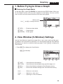
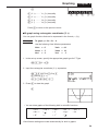
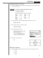
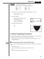
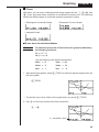
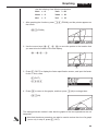
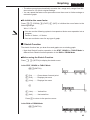
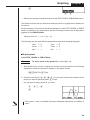
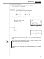
Chapter
4
Graphing
A collection of versatile graphing tools plus a large 79 × 47-dot
display makes it easy to draw a variety of function graphs quickly
and easily. This calculator is capable of drawing the following types
of graphs.
• Rectangular coordinate (Y =) graphs
• Parametric graphs
• Inequality graphs
• A selection of graph commands also makes it possible to incorporate graphing into programs.
1.
2.
3.
4.
5.
Before Trying to Draw a Graph
View Window (V-Window) Settings
Graph Function Operations
Drawing Graphs Manually
Other Graphing Functions
Graphing
Chapter 4
1. Before Trying to Draw a Graph
k Entering the Graph Mode
On the Main Menu, select the GRAPH icon and enter the GRAPH Mode. When you
do, the Graph Function (G-Func) menu appears on the display. You can use this
menu to store, edit, and recall functions and to draw their graphs.
Memory area
Use f and c to change selection.
1
2
3
4
1 (SEL) ........ Draw/non-draw status
2 (DEL) ....... Graph delete
4 (DRAW).... Draws graph
2. View Window (V-Window) Settings
Use the View Window to specify the range of the x-and y-axes, and to set the spacing between the increments on each axis. You should always set the View Window
parameters you want to use before drawing a graph. Press ! 3 to display the
View Window.
1. Press !3 to display the View Window.
!3(V-Window)
1
2
3
4
1 (INIT) ........ View Window initial settings
2 (TRIG) ...... View Window initial settings using specified angle unit
3 (Sto) ......... Store View Window settings to View Window memory.
4 (Rcl) ......... Recall View Window settings from View Window memory.
Xmin ............... Minimum x-axis value
Xmax .............. Maximum x-axis value
Xscl ................ Spacing of x-axis increments
48
Graphing
Chapter 4
2. Input a value for a parameter and press w. The calculator automatically selects
the next parameter for input.
• You can also select a parameter using the c and f keys.
Ymin ............... Minimum y-axis value
Ymax .............. Maximum y-axis value
Yscl ................ Spacing of y-axis increments
The following illustration shows the meaning of each of these parameters.
Y max
X min
(x, y)
X scl
Y scl
X max
Y min
3. Input a value for a parameter and press w. The calculator automatically selects
the next parameter for input.
• There are actually nine View Window parameters. The remaining three parameters appear on the display when you move the highlighting down past the Y
scale parameter by inputting values and pressing c.
Tmin ............... T minimum values
Tmax .............. T maximum values
Tptch .............. T pitch
The following illustration shows the meaning of each of these parameters.
min
ptch
(X, Y )
max
49
Graphing
Chapter 4
4. To exit the View Window, press Q.
• Pressing w without inputting any value also exits the View Window.
• The following is the input range for View Window parameters.
–9.99E+97 to 9.999E+97
• You can input parameter values up to 7 digits long. Values greater than 106 or
less than 10-1, are automatically converted to a 4-digit mantissa (including negative sign) plus a 2-digit exponent.
• The only keys that enabled while the View Window is on the display are: a to
j, ., E, -, f, c, d, e, +, -, *, /, (, ), ! 7,
Q. You can use - or - to input negative values.
• The existing value remains unchanged if you input a value outside the allowable range or in the case of illegal input (negative sign only without a value).
• Inputting a View Window range so the min value is greater than the max value,
causes the axis to be inverted.
• You can input expressions (such as 2π) as View Window parameters.
• When the View Window setting does not allow display of the axes, the scale for
the y-axis is indicated on either the left or right edge of the display, while that for
the x-axis is indicated on either the top or bottom edge.
• When View Window values are changed, the graph display is cleared and the
newly set axes only are displayed.
• View Window setting may cause irregular scale spacing.
• Setting maximum and minimum values that create too wide of a View Window
range can result in a graph made up of disconnected lines (because portions of
the graph run off the screen), or in graphs that are inaccurate.
• The point of deflection sometimes exceeds the capabilities of the display with
graphs that change drastically as they approach the point of deflection.
• Setting maximum and minimum values that create to narrow of a View Window
range can result in an error (Ma ERROR).
k Initializing and Standardizing the View Window
uTo initialize the View Window
a. Press !3 (V-Window) 1 (INIT) to initialize the View Window to the following
settings.
Xmin
= –3.9
Ymin
= –2.3
Xmax
= 3.9
Ymax
= 2.3
Xscl
= 1
Yscl
= 1
50
Graphing
Chapter 4
b. Press ! 3 (V-Window) 2 (TRIG) to initialize the View Window to the following settings.
Deg Mode
Xmin
= –360
Ymin
= –1.6
Xmax
= 360
Ymax
= 1.6
Xscl
=
Yscl
= 0.5
90
Rad Mode
Xmin
= –6.28318
Xmax
= 6.28318
Xscl
= 1.57079
Gra Mode
Xmin
= –400
Xmax
= 400
Xscl
= 100
• The settings for Ymin, Ymax, Ypitch, Tmin, Tmax, and Tpitch remain unchanged
when you press 2 (TRIG).
k View Window Memory
You can store a set of View Window settings in View Window memory for recall when
you need them.
uTo save View Window settings
While the View Window setting screen is on the display, press 3 (Sto) to save the
current settings.
• Whenever you save View Window settings, any settings previously stored in
memory are replaced.
uTo recall View Window settings
While the View Window setting screen is on the display, press 4 (Rcl) to recall the
View Window settings stored in memory.
• Whenever you recall View Window settings, the settings on the View Window are
replaced by the recalled settings.
• You can change View Window settings in a program using the following syntax.
View Window [Xmin value], [Xmax value], [Xscl value],
[Ymin value], [Ymax value], [Yscl value],
[Tmin value], [Tmax value], [Tptch value]
51
Graphing
Chapter 4
3. Graph Function Operations
You can store up to 10 functions in memory. Functions in memory can be edited,
recalled, and graphed. The types of functions that can be stored in memory are:
rectangular coordinate functions, parametric functions, and inequalities.
k Specifying the Graph Type
Before you can store a graph function in memory, you must first specify its graph
type.
1. While the Graph Function Menu is on the display, press [ to display a Graph
Type Menu.
[
1 (Y =) ......... Rectangular coordinate graph
[
1
2
3
4
1
2
3
4 [
2 (Parm) ...... Parametric graph
[
1 (Y >) ......... Y > f (x) inequality
2 (Y <) ......... Y < f (x) inequality
3 (Y ≥) ......... Y > f (x) inequality
4 (Y ≤) ......... Y < f (x) inequality
Press [ to return to the previous menu
2. Press the function key that corresponds to the graph type you want to specify.
k Storing Graph Functions
u To store a rectangular coordinate function (Y =)
Example
To store the following expression in memory area Y1:
y = 2 x2 – 5
[1(Y =)
(Specifies rectangular coordinate
expression.)
cTx-f
(Inputs expression.)
w
(Stores expression.)
52
Graphing
Chapter 4
• You will not be able to store the expression in an area that already contains a
parametric function. Select another area to store your expression or delete the
existing parametric function first. This also applies when storing inequalities.
u To store a parametric function
Example
To store the following functions in memory areas Xt2 and Yt2:
x = 3 sin T
y = 3 cos T
[2(Parm)
(Specifies parametric expression.)
dsTw
(Inputs and stores x expression.)
dcTw
(Inputs and stores y expression.)
• You will not be able to store the expression in an area that already contains a
rectangular coordinate expression or inequality. Select another area to store your
expression or delete the existing expression first.
u To store an inequality
Example
To store the following inequality in memory area Y3:
y > x2 – 2x – 6
[[1(Y>)
(Specifies an inequality.)
Tx-cT-g
(Inputs expression.)
w
(Stores expression.)
53
Graphing
Chapter 4
k Editing Functions in Memory
u To edit a function in memory
Example
To change the expression in memory area Y1 from y = 2x2 – 5
to y = 2 x2 – 3
e
(Displays cursor.)
eeeed
(Changes contents.)
w
(Stores new graph function.)
u To delete a function
1. While the Graph Function Menu is on the display, press f or c to display the
cursor and move the highlighting to the area that contains the function you want
to delete.
2. Press 2 (DEL).
1
2
3
4
3. Press 1 (YES) to delete the function for 4 (NO) to abort the procedure without deleting anything.
k Drawing a Graph
Before actually drawing a graph, you should first make the draw/non-draw status.
u To specify the draw/non-draw status of a graph
You can specify which functions out of those stored in memory should be used for a
draw operation.
• Graphs for which there is no draw/non-draw status specification are not drawn.
Example
To select the following functions for drawing:
Y1 : y = 2 x 2 – 5
X t 2: x = 3 sin T
Yt 2 : y = 3 cos T
54
Graphing
Chapter 4
Use the following View Window parameters.
Xmin
= –5
Ymin
= –5
Xmax = 5
Ymax = 5
Xscl
Yscl
= 1
= 1
ccc
(Select a memory area that contains a
function for which you want to specify
non-draw.)
1
2
3
4
1
Unhighlights
2
3
4
1(SEL)
(Specify non-draw.)
4(DRAW) or w
(Draws graphs.)
• Pressing u or A returns to the Graph Function Menu.
• A parametric graph will appear coarse if the settings you make in the View
Window cause the pitch value to be too large, relative to the differential between the min and max settings. If the settings you make cause the pitch value
to be too small relative to the differential between the min and max settings, on
the other hand, the graph will take a very long time to draw.
4. Drawing Graphs Manually
After you select the RUN icon in the Main Menu and enter the RUN Mode, you can
draw graphs manually. First press ! 4 (SKTCH) 2 (GRPH) to recall the Graph
Command Menu, and then input the graph function.
!4(SKTCH)2(GRPH)
1 (Y =) ......... Rectangular coordinate graph
1
2
3
4
2(Parm) ....... Parametric graph
55
[
Graphing
Chapter 4
[
1 (Y >) ......... Y > f (x) inequality
1
2
3
4 [
2 (Y <) ......... Y < f (x) inequality
3 (Y ≥) ......... Y > f (x) inequality
4 (Y ≤) ......... Y < f (x) inequality
Press [ to return to the previous menu.
u To graph using rectangular coordinates (Y =)
You can graph functions that can be expressed in the format y = f (x).
To graph y = 2x2 + 3x – 4
Example
Use the following View Window parameters.
Xmin
= –5
Ymin
= –10
Xmax = 5
Ymax = 10
Xscl
Yscl
= 2
=
5
1. In the set-up screen, specify the appropriate graph type for F-Type.
!Z1(Y =)Q
2. Input the rectangular coordinate (Y =) expression.
A!4(SKTCH)1(Cls)w
2(GRPH)1(Y =)
cTx+dT-e
3. Press w to draw the graph.
w
• You can draw graphs of the following built-in scientific functions.
• sin x
• cos x
• tan x
• sin –1 x
• cos–1 x
• tan–1 x
•
• x2
• log x
• lnx
• 10x
• ex
• x–1
•3
View Window settings are made automatically for built-in graphs.
56
Graphing
Chapter 4
u To graph parametric functions
You can graph parametric functions that can be expressed in the following format.
(X, Y) = ( f (T), g (T))
Example
To graph the following parametric functions:
x = 7 cos T – 2 cos 3T
y = 7 sin T – 2 sin 3T
Use the following View Window parameters.
Xmin
Xmax
Xscl
Tmin
Tptch
= –20
= 20
=
5
=
0
= π÷36
Ymin
Ymax
Yscl
Tmax
= –12
= 12
=
5
= 2π
1. In the set-up screen, specify the appropriate graph type for F-Type.
!Z2(Parm)
2. Set the default angle unit to radians (Rad).
cc2(Rad)Q
3. Input the parametric functions.
A!4(SKTCH)1(Cls)w
2(GRPH)2(Parm)
hcT-ccdT,
hsT-csdT)
4. Press w to draw the graph.
w
u To graph inequalities
You can graph inequalities that can be expressed in the following four formats.
• y > f (x)
• y < f (x)
• y > f (x)
• y < f (x)
57
Graphing
Example
Chapter 4
To graph the inequality y > x2 – 2x – 6
Use the following View Window parameters.
Xmin
= –6
Ymin
= –10
Xmax = 6
Ymax = 10
Xscl
Yscl
= 1
=
5
1. In the set-up screen, specify the appropriate graph type for F-Type.
!Z[1(Y>)Q
2. Input the inequality.
A!4(SKTCH)1(Cls)w
2(GRPH)[1(Y>)
Tx-cT-g
3. Press w to draw the graph.
w
5. Other Graphing Functions
The functions described in this section tell you how to read the x- and y-coordinates
at a given point, and how to zoom in and zoom out on a graph.
• These functions can be used with rectangular coordinate, parametric, and inequality graphs only.
k Connect Type and Plot Type Graphs (D-Type)
P.7
You can use the D-Type setting of the set-up screen to specify one of two graph
types.
• Connect type (Conct)
Points are plotted and connected by lines to create a curve.
• Plot
Points are plotted without being connected.
58
Graphing
Chapter 4
k Trace
With trace, you can move a flashing pointer along a graph with the f, c, d, and
e cursor keys and obtain readouts of coordinates at each point. The following
shows the different types of coordinate readouts produced by trace.
• Rectangular Coordinate Graph
• Parametric Function Graph
• Inequality Graph
u To use trace to read coordinates
Example
To determine the points of intersection for graphs produced by
the following functions:
Y1: y = x2 – 3
Y2: y = –x + 2
Use the following View Window parameters.
Xmin
= –5
Ymin
= –10
Xmax = 5
Ymax = 10
Xscl
Yscl
= 1
=
2
1. After drawing the graphs, press 1 (TRCE) to make the pointer appear at the far
left of the graph.
1(TRCE)
• The pointer may not be visible on the graph when you press 1 (TRCE).
2. Use e to move the pointer to the first intersection.
e~e
x/ y coordinate values
59
Graphing
Chapter 4
• Pressing d and e moves the pointer along the graph. Holding down either
key moves the pointer at high speed.
3. Use f and c to move the pointer between the two graphs.
4. Use e to move the pointer to the other intersection.
e~e
• To quit the trace operation, press 1 (TRCE) again.
uScrolling
When the graph you are tracing runs off the display along either the x- or y-axis,
pressing the e or d cursor key causes the screen to scroll in the corresponding
direction eight dots.
• You can scroll only rectangular coordinate and inequality graphs while tracing.
You cannot scroll parametric function graphs.
• Trace can be used only immediately after a graph is drawn. It cannot be used
after changing the settings of a graph.
• You cannot incorporate trace into a program.
• You can use trace on a graph that was drawn as the result of an output command (^), which is indicated by the “-Disp-” indicator on the screen.
k Scroll
You can scroll a graph along its x- or y-axis. Each time you press f, c, d, or
e, the graph scrolls 12 dots in the corresponding direction.
k Overwrite
Using the following syntax to input a graph causes multiple versions of the graph to
be drawn using the specified values. All versions of the graph appear on the display
at the same time.
<function with one variable> , ! [ <variable name> ! =
<value> , <value> , .... <value> ! ] w
60
Graphing
Example
Chapter 4
To graph y = A x2 – 3, substituting 3, 1, and –1 for the value of A
Use the following View Window parameters.
Xmin
= –5
Ymin
= –10
Xmax = 5
Ymax = 10
Xscl
Yscl
= 1
=
2
[1(Y =)
(Specifies graph type.)
aATx-d,
![aA!=d,
1
2
3
4
b,-b!]w
(Stores expression.)
4(DRAW) or w
(Draws graph.)
↓
↓
• The function that is input using the above syntax can have only one variable.
• You cannot use X, Y or T as the variable name.
• You cannot assign a variable to the variable in the function.
P.8
• When the set-up screen’s Simul-G item is set to “On,” the graphs for all the variables are drawn simultaneously.
61
Graphing
Chapter 4
k Zoom
The zoom feature lets you enlarge and reduce a graph on the display.
u Before using zoom
Immediately after drawing a graph, press !2 (ZOOM) to display the Zoom Menu.
!2(ZOOM)
1
2
3
4 [
3
4
1 (BOX) ....... Graph enlargement using box zoom
2 (FACT) ..... Displays screen for specification of zoom factors
3 (IN) ........... Enlarges graph using zoom factors
4 (OUT) ....... Reduces graph using zoom factors
[
1
1 (ORIG) ..... Original size
2
[
Press [ to return to the previous menu
uTo use box zoom
With box zoom, you draw a box on the display to specify a portion of the graph, and
then enlarge the contents of the box.
Example
To use box zoom to enlarge a portion of the graph y = (x + 5)
(x + 4) (x + 3)
Use the following View Window parameters.
Xmin
= –8
Ymin
= –4
Xmax = 8
Ymax = 2
Xscl
Yscl
= 2
= 1
1. After graphing the function, press !2 (ZOOM).
!2(ZOOM)
1
2
3
4
62
Graphing
Chapter 4
2. Press 1 (BOX), and then use the cursor keys (d, e, f, c) to move the
pointer to the location of one of the corners of the box you want to draw on the
screen. Press w to specify the location of the corner.
1(BOX)
d ~ dw
3. Use the cursor keys to move the pointer to the location of the corner that is diagonally across from the first corner.
f~fd~d
4. Press w to specify the location of the second corner. When you do, the part of
the graph inside the box is immediately enlarged so it fills the entire screen.
w
• To return to the original graph, press 2 (ZOOM) [ 1 (ORIG).
• Nothing happens if you try to locate the second corner at the same location or
directly above the first corner.
• You can use box zoom for any type of graph.
u To use factor zoom
With factor zoom, you can zoom in or zoom out on the display, with the current
pointer location being at the center of the new display.
• Use the cursor keys (d, e, f, c) to move the pointer around the display.
Example
Graph the two functions below, and enlarge them five times in
order to determine whether or not they are tangential:
Y1: y = (x + 4) (x + 1) (x – 3)
Y2: y = 3x + 22
63
Graphing
Chapter 4
Use the following View Window parameters.
Xmin
= –8
Ymin
= –30
Xmax = 8
Ymax = 30
Xscl
Yscl
= 5
= 10
1. After graphing the functions, press !2 (ZOOM), and the pointer appears on
the screen.
!2(ZOOM)
2. Use the cursor keys (d, e, f, c) to move the pointer to the location that
you want to be the center of the new display.
d~df~f
1
2
3
4
3. Press 2 (FACT) to display the factor specification screen, and input the factor
for the x- and y-axes.
2(FACT)
fwfw
4. Press Q to return to the graphs, and then press 3 (IN) to enlarge them.
Q3(IN)
This enlarged screen makes it clear that the graphs of the two expressions are not
tangential.
• Note that the above procedure can also be used to reduce the size of a graph
(zoom out). In step 4, press 4 (OUT).
64
Graphing
Chapter 4
• The above procedure automatically converts the x-range and y-range View Window values to 1/5 of their original settings.
• You can repeat the factor zoom procedure more than once to further enlarge or
reduce the graph.
u To initialize the zoom factor
Press ! 2 (ZOOM) 2 (FACT) 1 (INIT) to initialize the zoom factor to the
following settings.
Xfct = 2 Yfct = 2
• You can use the following syntax to incorporate a factor zoom operation into a
program.
Factor <X factor>, <Y factor>
• You can use factor zoom for any type of graph.
k Sketch Function
The sketch function lets you draw lines and graphs on an existing graph.
• Note that Sketch function operation in the STAT, GRAPH or TABLE Mode is
different from Sketch function operation in the RUN or PRGM Mode.
u Before using the Sketch Function
Press ! 4 (SKTCH) to display the sketch menu.
In the STAT, GRAPH or TABLE Mode
!4(SKTCH)
1 (Cls) ......... Clears drawn line and point
1
2
3
4
[
1
2
3
4
[
1
2
3
4 [
3 (Plot) ........ Displays plot menu
4 (Line) ........ Displays line menu
[
1 (Vert) ........ Vertical line
2 (Hztl) ........ Horizontal line
Press [ to return to the previous menu
In the RUN or PRGM Mode
!4(SKTCH)
65
Graphing
Chapter 4
[
1
2
3
4
• Other menu items are identical to those in the STAT, GRAPH, TABLE Mode menu.
The Sketch function lets you draw lines and plot points on a graph that is already on
the screen.
All the examples in this section that show operations in the STAT, GRAPH or TABLE
Mode are based on the assumption that the following function has already been
graphed in the GRAPH Mode.
Memory Area Y1: y = x(x + 2)(x – 2)
The following are the View Window parameters used when drawing the graph.
Xmin
= –5
Ymin
= –5
Xmax
= 5
Ymax
= 5
Xscl
= 1
Yscl
= 1
u To plot points
In the STAT, GRAPH or TABLE Mode
Example
To plot a point on the graph of y = x( x + 2)(x – 2)
1. After graphing the function, display the sketch menu and perform the following
operation to cause the pointer to appear on the graph screen.
!4(SKTCH)3(Plot)
2. Use the cursor keys (f, c, d, e) to move the pointer the locations of the
points you want to plot and press w to plot.
• You can plot as many points as you want.
e ~ ef ~ f
w
• The current x- and y-coordinate values are assigned respectively to variables X
and Y.
66
Graphing
Chapter 4
In the RUN or PRGM Mode
The following is the syntax for plotting points in these modes.
Plot < x-coordinate>, <y-coordinate>
Example
To plot a point at (2, 2)
Use the following View Window parameters.
Xmin
= –5
Ymin
= –10
Xmax = 5
Ymax = 10
Xscl
Yscl
= 1
=
2
1. After entering the RUN Mode, display the sketch menu and perform the following
operation.
!4(SKTCH)1(Cls)w
3(Plot)c,c
1
2
3
4
2. Press w.
ww
• You can use the cursor keys (f, c, d, e) to move the pointer around the
screen.
• If you do not specify coordinates, the pointer is located in the center of the
graph screen when it appears on the display.
• If the coordinates you specify are outside the range of the View Window parameters, the pointer will not be on the graph screen when it appears on the
display.
• The current x- and y-coordinate values are assigned respectively to variables
X and Y.
67
Graphing
Chapter 4
u To draw a line between two plotted points
In the STAT, GRAPH or TABLE Mode
Example
To draw a line between the two points of inflection on the graph
of y = x(x + 2)(x – 2)
Use the same View Window parameters as in the example on page
66.
1. After graphing the function, display the sketch menu and perform the following
operation to cause the pointer to appear on the graph screen.
!4(SKTCH)3(Plot)
2. Use the cursor keys (f, c, d, e) to move the pointer to one of the points
of inflection and press w to plot it.
d ~ df ~ f
w
3. Use the cursor keys to move the pointer to the other point of inflection.
e ~ ec ~ c
4. Display the sketch menu and perform the following operation to draw a line between the two points.
!4(SKTCH)4(Line)
68
Graphing
Chapter 4
In the RUN or PRGM Mode
Example
To draw a line perpendicular to the x-axis from point (x, y) = (2, 6)
on the graph y = 3x
Use the following View Window parameters:
Xmin
= –2
Ymin
= –2
Xmax = 5
Ymax = 10
Xscl
Yscl
= 1
=
2
1. After drawing the graph, use the procedure under “To plot points” to move the
pointer to (x, y) = (2, 0), then use the cursor key (f) to move the pointer on the
graph y = 3x.
!4(SKTCH)3(Plot)
c,awwf~f
2. Display the sketch menu and perform the following operation to draw a straight
line between the two points.
u
!4(SKTCH)4(Line)w
• The above draws a straight line between the current pointer location and the
previous pointer location.
u To draw vertical and horizontal lines
The procedures presented here draw vertical and horizontal lines that pass through
a specific coordinate.
In the STAT, GRAPH or TABLE Mode
Example
To draw a vertical line on the graph of y = x(x + 2)(x – 2)
1. After graphing the function, display the sketch menu and perform the following
operation to display the pointer and draw a vertical line through its current location.
!4(SKTCH)[1(Vert)
69
Graphing
Chapter 4
2. Use the d and e cursor keys to move the line left and right, and press w to
draw the line at the current location.
e ~ ew
• To draw a horizontal line, simply press 2 (Hztl) in place of 1 (Vert), and use
the f and c cursor keys to move the horizontal line on the display.
In the RUN or PRGM Mode
The following is the syntax for drawing vertical and horizontal lines in these modes.
• To draw a vertical line
Vertical <x-coordinate>
• To draw a horizontal line
Horizontal < y-coordinate>
uTo clear drawn lines and points
The following operation clears all drawn lines and points from the screen.
In the STAT, GRAPH or TABLE Mode
Lines and points drawn using sketch menu functions are temporary. Display the
sketch menu and press 1 (Cls) to clear drawn lines and points, leaving only the
original graph.
In the RUN or PRGM Mode
The following is the syntax for clearing drawn lines and points, as well as the graph
itself.
Cls EXE
70