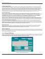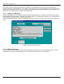
1
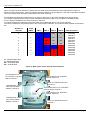
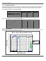
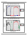
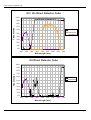
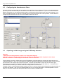
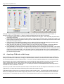
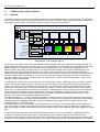
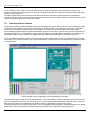
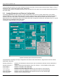
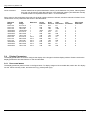
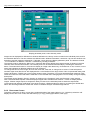
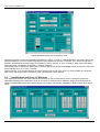
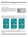
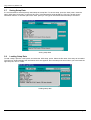
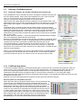
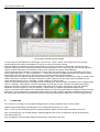
Using a FLIM ready Radiance MP 9MRC60UM11 Issue 1 Page 1 Using a FLIM ready Radiance MP Table of Contents 1 2 3 Introduction ...................................................................................................................... 2 Pre-requisites ................................................................................................................... 2 system components ......................................................................................................... 3 3.1 FLIM ready components .............................................................................................. 3 3.2 Bi-alkali vs. Multi-alkali................................................................................................. 4 3.3 Channel configurations ................................................................................................ 4 3.4 Direct Detector Filters .................................................................................................. 7 3.4.1 Bi-Alkali / BiAlkali configurations (BB) .................................................................. 7 3.4.2 Bi-Alkali/Multi-alkali configurations (BM) .............................................................. 7 3.4.3 Filter Diagrams ..................................................................................................... 7 4 How to use lasersharp2000 with flim detectors ............................................................. 10 4.1 Suitable methods for FLIM......................................................................................... 10 4.2 Configuring the direct detector filters......................................................................... 11 4.3 Acquiring a visible image using the FLIM ready detectors ........................................ 11 4.4 Acquiring a FLIM and a visible image........................................................................ 12 5 FLIM Data Acquisition in Detail...................................................................................... 13 5.1 General ...................................................................................................................... 13 5.2 Data Acquisition Software.......................................................................................... 14 5.3 Imaging Parameters and Detector Configuration ...................................................... 15 5.4 Display Parameters ................................................................................................... 16 5.4.1 Displaying Images .............................................................................................. 16 5.4.2 Displaying Curves............................................................................................... 17 5.5 Time Windows and Scan Y/Y Windows .................................................................... 18 5.6 Measurement Control ................................................................................................ 19 5.7 Saving Setup Data..................................................................................................... 20 5.8 Loading Setup Data ................................................................................................... 20 5.9 Running a FLIM Measurement .................................................................................. 21 5.9.1 Detector Control via the DCC-100 Detector Controller ...................................... 21 5.10 FLIM Data Acquisition................................................................................................ 21 5.11 Saving a FLIM Image................................................................................................. 22 5.12 Loading a FLIM Image............................................................................................... 23 5.13 FLIM Data Analysis.................................................................................................... 23 6 Literature ........................................................................................................................ 24 1 INTRODUCTION This manual is intended to be a supplement to a variety of other user manuals available for the use of the Radiance or the Becker & Hickl systems. For more detailed information on the use of these systems please refer to the following documents. Becker & Hickl documentation: SPC-830 Based TCSPC FLIM Systems for Radiance2100 – Quick Guide DCC100 – User manual for the DCC-100 detector control manual spc800ps – User manual for the Time-correlated Single Photon Counting Modules and Multi SPC software Bio-Rad documentation: 9m60um03 - Main Radiance operating manual 9m60um04 – Radiance MP operating manual LaserSharp2000 Help file 2 PRE-REQUISITES To use the Becker & Hickl Time-correlated Single Photon Counting Modules to perform FLIM on the Radiance you will need a FLIM ready Radiance system. It is possible to order new FLIM ready systems or upgrade older Radiance systems to be FLIM ready. There are a number of computer pre-requisites in order to use a single computer to run both 9MRC60UM11 Issue 1 Page 2 Using a FLIM ready Radiance MP the LaserSharp2000 acquisition software, the DCC-100 gain control software and the TCSPC software. (Note: if the Radiance system is supplied as FLIM ready these pre-requisites will be met). Dell Poweredge 1400, Dell Optiplex GX240 or Dell Optiplex GX260 PC or later Bio-Rad recommended model Windows 2000 At least 512Mb RAM At least 1Ghz processor (However, if the data analysis (SPCImage) is to be performed on the same machine a processor with 2GHz or more would be much better) One free full length PCI slot Additional two free half or full length PCI slots (except if the PC has a USB connector, and also has a PCI slot position taken up by an additional RS232 port adaptor, where only one other free PCI slot is required) In addition to these pre-requisites it is also highly recommended that if you intend to run the Multi-SPC software at the same time as LaserSharp2000 that you run a dual monitor setup. 3 SYSTEM COMPONENTS 3.1 FLIM ready components A FLIM ready system or upgrade includes the following: One or two Hamamatsu fast PMT assemblies, to replace existing Electron Tubes PMT tube assembly(ies). The PMTs will be either Bi or Multi-alkali (more details later) Corresponding FLIM preamplifier PCB(s), to replace existing One rear DDS panel, to replace existing channel 1+2 rear panel One DCC-100 PCI control card in PC (supports max 2 FLIM PMT tubes) DCC-100 Control Software Cables between DCC-100 card and FLIM PMTs If there is only one serial (RS232) connector on the PC, a USB to RS232 serial cable adaptor and associated driver Figure 1 - Example of PCI board configuration when running FLIM from a single computer 9MRC60UM11 Issue 1 Page 3 Using a FLIM ready Radiance MP 15W Female Dee - to DDS channel 1 PMT (if FLIM) 15W Female Dee to DDS channel 2 PMT (if FLIM) FLIM DCC-100 PCI Board ▼ Unibrain Firewire PCI Board (Supplied by Bio-Rad)▼ 15W Female Dee- to ICU triggering port (cable supplied by B&H) 15W Female Dee- to FLIM Electronics Box (cable supplied by B&H) FLIM SPC-830 PCI Board (supplied by B&H) ▲▼ SMA- to IR laser SYNC (cable supplied by B&H) SMA- to FLIM electronics box CFD (cable supplied by B&H) 3.2 Bi-alkali vs. Multi-alkali A Radiance Multi-photon system fitted with direct detectors may have either two or four channels. There are two types of PMT that may be used in the direct detectors: • Bi-Alkali (B) • Multi-Alkali (M) The only difference between the tubes is that the bi-alkali tube have higher quantum efficiency at the blue end of the spectrum and multi-alkali are better at the red end of the spectrum. The cross over where multi alkali performance becomes better than bi-alkali performance is around the 500 to 540nm range and higher. If you wish to confirm the type of alkali of a PMT in the direct detectors you can look at the rear of the detector unit. Bialkali tubes are marked with a blue dot and multi-alkali tubes with a red dot. Bi-alkali and Multi-alkali options exist for both traditional imaging PMTs and FLIM PMTs. 3.3 Channel configurations The 2 channel direct detectors have a very simple optical configuration. The emitted light is split by a single filter cube and the light is sent into one or both of the PMTs. Figure 2 - Two channel Direct detectors coupled to an Olympus BX50WI upright microscope 9MRC60UM11 Issue 1 Page 4 Using a FLIM ready Radiance MP Figure 3 - Optical Configuration for Two Channel Direct Detectors Emission 1 Emission 2 PMT2 PMT1 The shortest wavelength light is reflected into PMT1 and the longer wavelength light passes through the long pass (LP) dichroic into PMT2. The filter cube containing the dichroic and the emission filters is a relatively standard ‘Olympus’ block. 9MRC60UM11 Issue 1 Page 5 Using a FLIM ready Radiance MP Due to this split if a pair of detectors contains both a bi-alkali and a multi-alkali then the bi alkali will be in PMT1 to optimise system performance. Note this diagram has been rotated for ease of display: in the real configuration the PMTs are on top of each other with PMT1 at the bottom and PMT2 at the top. In the Radiance FLIM ready systems there is an option of either one or two PMTs suitable for FLIM acquisition. For a single FLIM detector the option is either a Bi-alkali FLIM detector (BF) or a multi-alkali FLIM detector (MF). If only a single FLIM detector is present it will be in channel 2. For a dual FLIM detector setup the options are either two bi-alkalis (BF-BF) or one of each (MF-BF) The same combinations are possible with the four channel direct detectors. This means that the possible combinations are: Number of channels FLIM PMT's PMT-1 PMT-2 PMT-3 PMT-4 2 1 B BF NA NA 2 2 BF BF NA NA 2 1 B MF NA NA 2 4 4 4 4 4 4 2 1 2 1 2 1 2 BF B BF B BF B BF MF BF BF BF BF MF MF NA B B M M M M NA M M M M M M Filter movement Manual or Motorised Manual or Motorised Manual or Motorised Manual or Motorised Motorised Motorised Motorised Motorised Motorised Motorised M = Standard Multi-alkali B = Standard Bi-alkali MF = FLIM Multi-alkali BF = FLIM Bi-alkali Figure 4 - Back panel of two channel direct detectors 15W Female Dee- to PC, FLIM DCC-100 PCI Board. Channel 2 15W Male Dee- control from ICU Dual DDS Module. Channel 2 SMB- signal to ICU, Dual DDS Module. Channel 2 SMA- to FLIM electronics box. Channel 2 15W Female Dee- to PC, FLIM DCC100 PCI Board. Channel 1 SMB- signal to ICU, Dual DDS Module. Channel 1 15W Male Dee- control from ICU Dual DDS Module. Channel 1 9MRC60UM11 SMA- to FLIM electronics box. Channel 1 Issue 1 Page 6 Using a FLIM ready Radiance MP 3.4 Direct Detector Filters The direct detector use large Olympus style filter blocks. The following tables show the typical filter blocks available with the Radiance Multi-photon systems. If these filters are not suitable then you may purchase an empty filter block and create another configuration. The emission 1 filters are in front of PMT1 and emission 2 filters are in front of PMT2. 3.4.1 BI-ALKALI / BIALKALI CONFIGURATIONS (BB) Olympus Filter Block Name Emission 1 HQ450/80 UG11/IR Open HQ390/70 Blue/Green (DAPI/ Fluorescein) UV/Visible (Serotonin/ Fluorescein) UV (Serotonin) Indo-1 3.4.2 Emission 2 HQ515/30 HQ575/150 UG11/IR HQ495/20 BI-ALKALI/MULTI-ALKALI CONFIGURATIONS (BM) Olympus Filter Block Name Emission 1 HQ450/80 HQ450/80 HQ515/30 UG11/IR UG11/IR HQ390/70 Blue/Green (DAPI/Fluorescein) Blue/Red (DAPI/Rhodamine) Green/Red (Fluorescein/Rhodamine) UV/Visible (Serotonin/ Fluorescein) UV (Serotonin) Indo-1 3.4.3 Filters Dichroic DC500LP UV400DCLP Open 440DCLPXR Filters Dichroic DC500LP DC500LP DC560LP UV400DCLP 670UVDCLP 440DCLPXR Emission 2 HQ515/30 HQ620/100 HQ620/100 HQ575/150 Open HQ495/20 FILTER DIAGRAMS The transmission curves for the main filter block types are shown below. In addition it is possible to use other filter blocks provided that they provide sufficient blocking of the IR laser. Blue / Green Direct Detector Cube 100% 90% 80% Transmission 70% 60% HQ450/80 HQ515/30 50% HQ495DCXR 40% 30% 20% 10% 0% 400 450 500 550 600 650 700 Wavelength (nm) 9MRC60UM11 Issue 1 Page 7 Using a FLIM ready Radiance MP Blue / Red Direct Detector Cube 100% 90% Transmission 80% 70% 60% HQ450/80 HQ620/100 50% HQ495DCXR 40% 30% 20% 10% 0% 400 450 500 550 600 650 700 Wavelength (nm) Green / Red Direct Detector Cube 100% 90% Transmission 80% 70% 60% HQ515/30 HQ620/100 50% 560DRLP 40% 30% 20% 10% 0% 400 450 500 550 600 650 700 Wavelength (nm) 9MRC60UM11 Issue 1 Page 8 Using a FLIM ready Radiance MP UV / Vis Direct Detector Cube 100% 90% Transmission 80% 70% 60% UG11IR HQ575/150 50% UV400DCLP 40% 30% 20% 10% 0% 300 350 400 450 500 550 600 650 700 Wavelength (nm) UV Direct Detector Cube 100% 90% Transmission 80% 70% 60% UG11IR 50% UV670DCLP 40% 30% 20% 10% 0% 300 350 400 450 500 550 600 650 700 Wavelength (nm) 9MRC60UM11 Issue 1 Page 9 Using a FLIM ready Radiance MP Indo Direct Detector Cube 100% 90% 80% Transmission 70% 60% D390/70 HQ495/20 50% UV440DCLP 40% 30% 20% 10% 0% 350 400 450 500 550 600 Wavelength (nm) 4 HOW TO USE LASERSHARP2000 WITH FLIM DETECTORS The FLIM ready Radiance can be used to collect a FLIM image, a visible image or both at the same time. 4.1 Suitable methods for FLIM When configuring methods for FLIM detection you will need to ensure that the FLIM detector(s) are in use in the methods. If you only have a single FLIM detector it will be detector number 2. 9MRC60UM11 Issue 1 Page 10 Using a FLIM ready Radiance MP 4.2 Configuring the direct detector filters When the method has been loaded it is possible to check the filter setup by going to the Tools > Carousel setup menu. By clicking on the various blocks you can determine the filters in front of the detectors. If you have a motorised direct detector setup then you can change the filter positions by clicking the left and right arrows above each detector. If you have a manual setup then you will have to actually have to move the wheels to the correct position. Further details on configuring the filter blocks can be found in the Radiance MP user manual. 4.3 Acquiring a visible image using the FLIM ready detectors Remarks: 1) Indicate more clearly that this section is for steady state imaging. 2) The DCC 100 is not longer used for the new systems. The gain is controlled only by the Laser sharp. Detector shutdown is indicated by an intermittend sound of the buzzer. The procedure to acquire a visible image using a FLIM detector is almost identical to acquire an image using the non FLIM direct detectors. Once you have created or loaded an appropriate method and checked the filters you then need to set the levels in the channels part of the control panel. The laser should initially be set to off, the iris slider is grey because there is no aperture for the direct detectors, the gain should be set to 1 and the offset to 0. In addition to the LaserSharp2000 software you will also need to be running the DCC-100 software. The gain control in LaserSharp2000 should remain at a level of 1 and you should control the gain level using the slider on the DCC-100 software. Gain for non-FLIM direct detectors you can use the gain slider in LaserSharp2000 as normal. Now you can slowly increase the laser power slider until you obtain a suitable image. 9MRC60UM11 Issue 1 Page 11 Using a FLIM ready Radiance MP Although it is good imaging practise to ensure that a PMT never saturates, the FLIM PMTs are more sensitive to saturation than the non-FLIM PMTs. In order to protect the PMTs there are five steps of protection: 1. The sample / objective lens of the sample should be shielded from stray light. This is especially important when collecting FLIM images. 2. Always start imaging with the gain low and the laser off, start scanning and then slowly increase the settings. For subtle changes use the spin buttons or when you have used a slider you can use the up and down arrows on the keyboard to change the values. 3. Although they are not aesthetically pleasing, look up tables (LUTs) like setcol and sethigh give users a visual indication of when the PMT is approaching saturation as red pixels start to appear. 4. When the PMTs are starting to run at the higher end of their collection range a speaker in the direct detector housing will start to emit a warning sound. This will increase in volume as the signal level increases. 5. If the FLIM detector receives too much signal a safety mechanism will cut off the gain to the system. This will be indicated in the DCC-100 software. In order to remedy the situation you should first remove or reduce the source of light down to acceptable levels. Then to reset the gain you need to set the gain to 0 in the LaserSharp2000 software and the DCC-100 software. Now set the gain in LaserSharp2000 to 1 and start increasing the DCC-100 gain until an image is visible. 4.4 Acquiring a FLIM and a visible image When collecting a visible image using the steps highlighted above the signal from the FLIM PMTs is also available for analysis in the Becker & Hickl boards. Simply run LaserSharp2000, the DCC-100 software and the Multi-SPC software for controlling the Becker & Hickl FLIM acquisition. There are a few tips regarding setting up the scanning parameters. When setting the box size in LaserSharp2000 you should consider the image resolution you wish to use for the FLIM image. Although these do not have to be the same size the FLIM image will either be the same size as the LaserSharp2000 scan area or a divided factor, i.e. if scanning at 512x512 in LaserSharp2000 the FLIM image can be collected at 512x512, 256x256 or 128x128. The zoom, pan and rotate commands should be used to fill the field of view with the sample and maximise the use of the FLIM memory. Be wary that the rate of bleaching will increase as increase the zoom. FLIM data analysis requires many more photons than a simple intensity image. This means that LaserSharp2000 will have to be configured to scan the same image many times in a row in order to provide the Becker & Hickl boards with enough photons. The easiest way to do this is to activate kalman filtering and to set an appropriate number of scans. 9MRC60UM11 Issue 1 Page 12 Using a FLIM ready Radiance MP 5 FLIM DATA ACQUISITION IN DETAIL 5.1 General FLIM data acquisition is based on a multi-dimensional time-correlated single photon counting technique, i.e. on building up the photon density over the time in the fluorescence decay, the coordinates of the scanning area, and the detector or wavelength channel number. The principle of this technique is shown in the figure below. Detectors Channel Channel register n Channel / Wavelength Router Timing Start Time Measurement CFD TAC Stop from Laser t ADC CFD Frame Sync Counter Y Line Sync Pixel Clock from Microscope Time within decay curve y Scanning Interface Counter X x Histogram Memory Detector channel 1 Histogram Memory Detector channel 2 Histogram Memory Detector channel 3 Histogram Memory Detector channel 4 Location within scanning area Multi-detector TCSPC lifetime imaging At the input of the system are several photomultipliers (PMTs), typically detecting in different wavelength intervals. The Radiance MP uses direct detector modules with one or two FLIM PMTs. The microscope can be equipped with two such detector modules. Consequently, the FLIM system can be operated with up to four detectors simultaneously. The detectors work in the photon counting mode, i.e. at a gain that gives an output pulse for each individual photon. The single photon pulses of the detectors are fed into the ‘router’. The router makes use of the fact that the detection of several photons in different detector channels in one laser period is unlikely. Therefore, the single photon pulses from all detector channels can be combined into a common photon pulse line and sent through the normal time measurement procedure of the TCSPC module. Simultaneously, the router delivers a channel number that indicates in which of the detectors a photon was detected. The subsequent TCSPC electronics consists of a time measurement channel, a scanning interface, a detector channel register, and a large histogram memory. The time measurement channel contains the usual TCSPC building blocks (CFDs, TAC, ADC) in the ‘reversed start-stop’ configuration. For each photon, it determines the detection time (t) with respect to the next laser pulse. The scanning interface is a system of counters which receive the scan control signals (frame sync, line sync and pixel clock) from the microscope. It determines the current location (x and y) of the laser spot in the scanning area. Synchronously with the detection of a photon, the detector channel number (n) for the current photon is read into the detector channel register. If the light is split into different wavelength intervals in front of the detectors n represents the wavelength of the detected photon. The obtained values for t, x, y and n are used to address the histogram memory in which the distribution of the photons over time, wavelength, and the image coordinates builds up. The result is a four dimensional data structure that contains separate blocks for the different wavelength intervals. Each block can be regarded as an image containing a full fluorescence decay curve in each pixel. The data acquisition runs at any desired scanning speed of the microscope. The data acquisition can be repeated as often as necessary to collect enough photons. Due to the synchronisation via the scan clock pulses, the regular zoom and image rotation functions of the microscope act automatically on the TCSPC recording and can be applied in the usual way. It should be pointed out that the used histogramming process does not use any time gating or wavelength scanning. Therefore, the method yields a near perfect counting efficiency and a maximum signal to noise ratio for a given fluorescence intensity and acquisition time. Due to the short dead time of the TCSPC imaging electronics (125 ns) there is virtually no loss of photons for count rates up to a few 105/s as they are typical for cell imaging. Moreover, the number 9MRC60UM11 Issue 1 Page 13 Using a FLIM ready Radiance MP of time channels of each pixel can be made large enough to obtain a sufficiently sample fluorescence decay curve. Therefore, fluorescence lifetimes far below 100 ps can be determined, and the components of double-exponential decay functions can be resolved. For details, please refer to the SPC-830 manual and the manuals of the HRT41 router and the DCC-100 detector controller. If you do not have these manuals, please download them from www.becker-hickl.com. Please find also a list of TCSPC and FLIM literature at the end of this manual. 5.2 Data Acquisition Software The general functions of the Biorad Radiance MP are controlled by the ‘Laser Sharp’ software. The FLIM data acquisition in the bh SPC-830 module is controlled by the ‘Multi SPC’ (SPCM) software. The FLIM detectors can be controlled by the bh DCC-100 detector controller and its ‘DCC’ software, or via the Laser Sharp software of the Radiance MP. The FLIM data acquisition delivers the photon distribution over the time on the ps scale and the scanning coordinates for the individual detectors. To obtain liftetime images from these data the recorded photon distribution is processed by the ‘SPCImage’ lifetime analysis software. For details, please find the individual manuals on www.becker-hickl.com. To run a FLIM data acquisition, start the Laser Sharp software, the SPCM software, and - if the detectors are controlled via the DCC-100 - the DCC software. The recommended screen cconfiguration of the SPCM and DCC software is shown in the figure below. Recommended screen configuration of the SPCM and DCC software The SPCM main panel contains the data display window, a count rate display, a status information window, and controls to set the acquisition time (Time) , the time scale (TAC), and the electrical input parameters (CFD and SYNC). Moreover, data can be recorded into and displayed from different memory pages (Meas. Page and Disp. Page). The SPCM software has a number of sub-panels. The most frequently used sub-panel in FLIM applications is the ‘Display Parameters’ panel. We recommend to keep the display parameters panel open all the time (upper right). 9MRC60UM11 Issue 1 Page 14 Using a FLIM ready Radiance MP The main panel of the DCC-100 control software is shown lower right. The DCC panel should be kept ‘always on top’ by activating on the corresponding button under ‘Parameters’. The data display window, the display parameter panel, and the DCC main panel can be resized and placed anywhere in the screen area. 5.3 Imaging Parameters and Detector Configuration The imaging parameters and the number of used FLIM detectors are set in the ‘System Parameters’ of the SPCM software. Moreover, the System Parameter panel contains a large number of other parameters controlling the internal functions of the SPC-830 module. The meaning of these parameters is described in the SPC-830 manual. Theses parameters are set to reasonable values in the default setup files coming with the SPC-830. Normally there is no need to change them for the Radiance MP FLIM system. The System Parameter panel is shown below. System Parameter panel of the SPCM software The parameters controlling the image configuration are located under ‘Data Format’, ‘Page Control’ and in the ‘More Parameters’ sub-panel. Routing Channels X: Routing Channels Y: Scan Pixels X: Scan Pixels X: Line Predivider: Pixel Clock divider: ADC Resolution: 9MRC60UM11 Number of FLIM detector channels used. Up to four detector channels can be used with the Radiance. Used for two-dimensional detector arrays only. Always ‘1’ for the Radiance FLIM system. Number of X pixels in the FLIM image Number of Y pixels in the FLIM image Several pixels of the Radiance 2100 scan can be binned into one FLIM pixel Number of lines of the Radiance scan binned into one line of the FLIM image Number of rows of the Radiance scan binned into one row of the FLIM image Number of time channels per pixel Issue 1 Page 15 Using a FLIM ready Radiance MP Count Increment: Number added into the photon distribution memory at the detection of a photon. Values greater than one may be used to avoid data extinction in the displayed images. (See SPC-830 manual) In SPCM versions of September 2003 or later ‘1’ is recommended. Due to memory size restrictions the product of the pixel numbers, detector channels, and time channels is limited. Some combinations of scan parameters are shown in the table below. Radiance Image 512 x 512 512 x 512 512 x 512 1024x1024 1024x1024 1024x1024 1024x1024 512 x 512 512 x 512 512 x 512 1024x1024 1024x1024 1024x1024 5.4 FLIM Image 512 x 512 256 x 256 128 x128 1024x1024 512 x 512 256 x 256 128 x 128 512 x 512 256 x 256 128 x128 512 x 512 256 x 256 128 x 128 Detectors 1 1 1 1 1 1 1 2 to 4 2 to 4 2 to 4 2 to 4 2 to 4 2 to 4 Scans Pixels X 512 256 128 1024 512 256 128 512 256 128 512 256 128 Scan Pixels Y 512 256 128 1024 512 256 128 512 256 128 512 256 128 ADC Resolution 64 256 1024 16 64 256 1024 16 64 256 16 64 256 Line Predivider 1 2 4 1 2 4 8 1 2 4 2 4 8 Pixel Clock Predivider 1 2 4 1 2 4 8 1 2 4 2 4 8 Display Parameters The display parameters are used to configure the display of the images in the data display window. Please note that the display parameters have no influence on the recorded data. 5.4.1 DISPLAYING IMAGES The display parameter panel is shown in the figure below. To display images of the recorded data, switch the ‘3D’ display into the ‘Colour-Intensity’ mode, and select the F(x,y) mode (lower right). 9MRC60UM11 Issue 1 Page 16 Using a FLIM ready Radiance MP Display parameter panel, colour-intensity mode Images can be displayed for different time windows defined on the decay curves recorded in the individual pixels, and for the individual detectors. The time windows are defined under ‘Window Parameters’, see below. Up to 8 time windows can be defined, and the images be selected by ‘T-Window’, lower right in the display parameter panel. The detector channel - or a combination of detetecor channels - is selected by ‘Routing X Window’. The intensity scale is selected by ‘Max Count’, upper left. Max Count defines the average number of photons in the time channels of the selected time window. The intensity scale can be selected automatically by activating the ‘autoscale’ button. The autoscale function is convenient to display an image under almost any circumstances. It can, however, not be used if the brightness of different images has to be compared. To change the colours of the image, click into the colour bar, lower left, or change ‘No of colours’. Pixels with photon numbers higher than ‘Max Count’ are displayed with a colour defined in the ‘High Colour’ field. Compared with teady stae imaging techniques, TCSPC has a much higher dynamic range. Therefore, if you have saturated pixels marked by ‘High Colour’ this need not mean that there is saturation in the recorded data. Changing Max Count is usually enough to display these pixels. The images can be flipped in X and Y direction by clicking on the ‘Reverse X scale’ and ‘Reverse Y scale’ buttons. Note: The SPCM data acqisition software displays images within slectable time windows - it does not display lifetime images. Lifetime images require to analyse the decay functions in the individual pixels to obtain the exponential ccomponents and intensity coefficients of the decay functions. Liftetime analysis is done by processing the SPCM data files in the SPCImage software. Please see section ‘FLIM Data Analysis’ and SPCImage manual. 5.4.2 DISPLAYING CURVES To display a sequence of decay curves along a selected stripe of the image (either in X or Y direction) switch the ‘3D’ display into the ‘3D curve’ mode, and select the F(t,x) or F(t,y) mode (figure below, lower right). 9MRC60UM11 Issue 1 Page 17 Using a FLIM ready Radiance MP Display parameter panel, 3D curve display mode Sequences of decay curves can be displayed for different ‘Scan X’ or ‘Scan Y’ windows defined in the image, and for the individual detectors. The scan windows are defined under ‘Window Parameters’, see below. Up to 8 Scan X and Scan Y windows can be defined, and the images be selected by ‘Scan X Window’ or ‘Scan Y Window’, lower right in the display parameter panel. The detector is selected by ‘Routing X Window’. The intensity scale is selected by ‘Max Count’, upper left. Max Count defines the average number of photons in the pixels of the selected ‘Scan X’ or ‘Scan Y’ window. Please note that, if you change between the colour intensity and the 3D curve mode, you have probably to change the ‘Max Count’ and the state of the ‘Reverse X scale’ and ‘Reverse Y scale’ buttons. 5.5 Time Windows and Scan Y/Y Windows The ‘Window Parameters’ are used to define time windows on the recorded decay curves in which the images are calculated and displayed. Furthermore, ‘Scan X’ and ‘Scan Y’ windows can be defined to display sequences of decay curves over selectable horizontal or vertical stripes of the image. The ‘Window Parameters’ panel is shown in the figure below. 9MRC60UM11 Issue 1 Page 18 Using a FLIM ready Radiance MP Window Parameters Please note that the available windows change with the ADC resolution, i.e. the number of points on the decay curves, and the x/y pixel numbers of the image. 5.6 Measurement Control The data recording in the SPC-830 module runs time-controlled. A ‘Collection Time’ defines the time for which the fluorescence photons are to be collected. After the start of the measurement, the SPC-830 module waits for the start of the next frame of the scan procedure, starts the acquisition, and acquires the photons of how many frames are scanned within the selected ‘Collection Time’. The collection time is set in the SPC ‘System Parameters’ or, more conveniently, in the lower left part of the main panel, see figure right. Defining the ‘Collection Time’ in the lower left part of the main panel The measurement control parameter section of the SPC ‘System Parameters’ is shown below. In the simplest case, a measurement runs over the defined ‘Collection Time’, then the measurement stops (figure below, left). In any case, the image is displayed in the style defined by the ‘Display Parameters’. For very long collection times it is recommended to run several ‘Cycles’, to accumulate the data, and to display the result at the end of each cycle. With the settings shown in the figure below (middle) 10 cycles of 30 seconds are accumulated. Single measurement of 30s, result displayed at the end 10 measurements of 30 s, data accumulated, result displayed each 30s A series of 10 subsequent measurements is run and the results are saved into data files A sequence of images can be recorded by using the ‘Autosave’ function, see figure above, right. 10 images, each of 30 seconds collection time, are acquired and automatically saved into subsequent data files. Other control parameters are available to record a fast sequence of small images by ‘Step’ function, or a to trigger a sequence or the steps of a sequence by an external signal, e.g. from the z scan of a microscope. Please see SPC-830 manual for details. 9MRC60UM11 Issue 1 Page 19 Using a FLIM ready Radiance MP 5.7 Saving Setup Data It is recommended to save frequently used setups as ‘setup files’. To save a setup, open the ‘Save’ panel, chose the option ‘SPC Setup’ and type in or select a file name. If the selected file exists already the ‘File Info’ window shows information about it. In the lower part of the ‘Save’ panel you can type in information about the setup to be saved. Saving setup data 5.8 Loading Setup Data To load a setup, open the ‘Load’ panel, and select the ‘SPC setup’ option. Select the file name of the setup to be loaded. The ‘File Info’ window displays the information which was typed in when the setup was saved. When you have found the right setup file, click on ‘Load’. Loading setup data 9MRC60UM11 Issue 1 Page 20 Using a FLIM ready Radiance MP 5.9 Running a FLIM Measurement 5.9.1 DETECTOR CONTROL VIA THE DCC-100 DETECTOR CONTROLLER The FLIM detectors can be controlled via a DCC-100 detector controller or directly from the Laser Sharp software. If both options are implemeted only one control should be used, i.e. the the detector gain in the unused control be set to zero. The DCC-100 panel can be placed anywhere in the screen area. After the start of the DCC application all DCC outputs are in the ‘Disabled’ state. This safety feature was built in to avoid unintentional activation of the detectors or of external high-voltage power supplies. To activate the detectors, click on the ‘Enable Outputs’ button. The detector gain is controlled by the Gain/HV sliders. Please note that for photon counting the sensitivity of the detectors cannot be reasonable changed by changing the detector gain. Reducing the gain of a detector in the photon counting mode results in reducing the detection efficiency, not the ‘gain’ of the recorded signal. For FLIM measurement we recommend to operate the detectors close to the maximum available gain, or 90 to 100%. For details of detector operation, or SPC-830 discriminator threshold and discriminator zero cross adjustment, please see SPC-830 manual. Because the FLIM detectors are used at high gain they can easily be overloaded, either by turning up the laser power too high, or by daylight leaking into the detection path. If overload occurs the DCC-100 detector controller shuts down the gain of the corresponding detector. Overload shutdown is indicated as shown in the figure right. If you get an overload shutdown, remove the reason of the overload, i.e. reduce the laser power or turn off the room lights, and click on the ‘Reset’ button. The detector then resumes normal operation. Detector control panel, detectors active Note: If you control the detector gain via the Laser Sharp software, overload shutdown is indicated by an intermittend buzz from the detector box. To reactivate the detector, turn down the detector gain to zero, and then re-set it to the gain previously used. Detector control panel, in overload shutdown state 5.10 FLIM Data Acquisition To start the FLIM data acquisition in the SPCM software start a continuous scan in the laser sharp software. When the scan is running, click on the ‘Start’ button on the top of the SPCM software. The data acquisition starts with the next frame of the scanning procedure and runs for the specified ‘Collection Time’. If you defined several ‘Cycles’ the measurement will repeat until the specified number of cycles has been completed. You can change the display parameters during the measurement without confusing the data acquisition. The changed parameters become active with the display of the next cycle. Although running a FLIM measurement is simple the advice given below should be obeyed: Run the system at a reasonable count rate Watch the count rate bars during the measurement. The most important rate is the TAC rate. (The displayed CFD rate can be higher than the actual photon rate because of ringing and afterpulsing, the ADC rate jumps up and down with the scanning.) Typical count rates for cells under two-photon excitation are in the range from 40.000 to 400.000 photons per second. The maximum count rate that can reasonable be recorded with the SPC-830 is 2 to 3 MHz. Please note that the displayed count rates are the average rates over the whole scanning area. If you have only a few bright spots on a large dark background the count rates in these spots can be substantially higher than displayed. If the rate drops significantly during the measurement photobleaching is on work, and the excitation power must be reduced. 9MRC60UM11 Issue 1 Count rate display Page 21 Using a FLIM ready Radiance MP Collect enough photons FLIM data analysis requires much more photons than a simple intensity image. Please keep in mind that you actually record a large number of images - one for each time channel defined by the ADC resolution. An intensity image looks reasonable good with 50 or 100 photons per pixel. Rough single exponential decay analysis requires 200 to 500 photons per pixel, precision single exponential analysis needs a few 1000 photon per pixel, and double exponential decay analysis 10,000 and more. The corresponding acquisition time range from 10 seconds to 10 or 20 minutes, depending on the available photon rate and the number of pixels. Therefore, be patient and get as many photons as you can. Avoid Photobleaching Due to the large number of fluorescence photons to be collected photobleaching is a severe problem in any FLIM measurement. For two-photon excitation photobleaching is nonlinear, i.e. increases more than linear with the absorption and emission rate. Most likely there is also a dependence on the excitation wavelength. All you can do to keep the photobleaching rate low is to use a low laser intensity and a correspondingly long acquisition time, and, if possible, to select a laser wavelength well inside the two-photon absorption band the fluorophores in your sample. Watch the TAC rate bars during the measurement.Typical count rates for cells under two-photon excitation are in the range from 40.000 to 400.000 photons per second. Please note that the displayed count rates are the average rates over the whole scanning area. If you have only a few bright spots on a large dark background the count rates in these spots can be substantially higher than displayed. If the rate drops significantly during the measurement the sample bleaches. This does not only reduce the number of photons you can get from your sample, it may also significantly change the lifetime distribution. Moreover, there may be highly reactive photobleaching products, and nobody knows whether or not these have an influence on the lifetime of the still functional fluorophore molecules or their binding state to the proteins in the cell. Set the right zoom Use the zoom function of the Laser Sharp software to fill the imaging area with the object to be imaged. This avoids waisting precious FLIM memory for dark image areas. Moreover, if you have only a few bright spots on a black background you do not get useful information about the count rate in these spots. Keep the daylight out Detection external light can cause a substantial background in the recorded fluorescence decays. In the data analysis the background has to be taken into account as an additional fitting parameter. Therefore a high background severely impairs the accuracy of the lifetime measurement. 5.11 Saving a FLIM Image When the measurement is finished, don’t forget to save the result into a file. Saving data works in a similar way as saving a setup. Open the ‘Save’ panel, and select the options ‘SPC data’ and ‘All used data sets’. Type in or select a file name. If the file already exists you get the file information displayed in the File Info window. Saving FLIM and system setup data 9MRC60UM11 Issue 1 Page 22 Using a FLIM ready Radiance MP Type in some useful information into the Author, Company or Contents fields, and click on ‘Save’ so save the file. The file contains the complete data set, i.e. the decay curves with the number of points defined by ‘ADC Resolution’ in all pixels of the FLIM image. Furthermore, the complete setup parameter set is saved with the data. You can load the data file later to run a measurement with identical setup parameters. 5.12 Loading a FLIM Image The SPC data files do not only contain the data but also the complete data set, i.e. the decay curves with the number of points defined by ‘ADC Resolution’ in all pixels of the FLIM image. You can load an SPC data file to run a measurement with parameters identical to that of an earlier measurement. To load the data and the setup, open the ‘Load’ panel, and select the option ‘SPC data’. Select the right file and click on ‘Load’. Loading FLIM and system setup data 5.13 FLIM Data Analysis The data sets saved by the SPCM software contain the fluorescence decay curves in the individual pixels. To convert these data into colour-coded lifetime images the bh ‘SPCImage’ software is used, see figure below. 9MRC60UM11 Issue 1 Page 23 Using a FLIM ready Radiance MP SPCImage FLIM data analysis software To import the SPC-830 data file into SPCImage, click into ‘File’, ‘Import’. Select ‘Scan Image’ and chose a ‘Page’ corresponding to the number of the detector for which you want to process the image. When the data are imported an intensity image appears in the upper left window of SPCImage. Set the cursor at a resonably bright spot of the image and look at the corresponding decay curve in the lower part of the SPCImage panel. Use the cursors of the decay curve window to select a time interval that contains reasonable data. The fit model for lifetime calculation is selected in the lower right area of SPCImage. It is recommended to start with a mono-exponential decay, i.e. ‘Exp. Components’ = 1. There are a number of fit parameters which can either be fixed or kept floating in the fitting procedure. We recommend to start with all the parameters floating. To get a good fit of the data the instrument response function (IRF) of the system must be known, which is usually not the case for two-photon excitation. Therefore a best-guess system response can (but need not) be calculated from the image data themselves. Click on ‘Calculate’, ‘System response’ to obtain an IRF. When you have managed to get a resonable fit for the selected pixel, start the lifetime calculation for the complete image. Click on ‘Calculate’, ‘Decay Matrix’, and wait. Depending on the image size, the calculation can take some minutes. When the calculation is finished a coloured lifetime image appears in the upper right window, along with a lifetime distribution over the image area. Click into ‘Options’, ‘Colour Coding’ to select an appropriate lifetime range. Much more functions are available in the SPCImage software, such as multi-exponential fits, arithmetic functions of the fit parameters. Typical applications of these advanced functions are FRET imaging, separation of different fluorophores in the same pixels, and probing cell parameters by lifetime sensitive fluorophores. Please refer to the SPCImage manual. 6 LITERATURE D.V. O’Connor, D. Phillips, Time Correlated Single Photon Counting, Academic Press, London (1984) Hidehiro Kume (Chief Editor), Photomultiplier Tube, Hamamatsu Photonics K.K., 1994 HRT-41, HRT-81, HRT-82 Routing Devices, Operating Manual. Becker & Hickl GmbH, www.becker-hickl.com SPC-134 through SPC-730 TCSPC Modules, Operating Manual and TCSPC Compendium. Becker & Hickl GmbH, www.becker-hickl.com DCC-100 Detector Control Module, Becker & Hickl GmbH, www.becker-hickl.com 9MRC60UM11 Issue 1 Page 24 Using a FLIM ready Radiance MP TCSPC Laser Scanning Microscopy - Upgrading laser scanning microscopes with the SPC-730 TCSPC lifetime imaging module, Becker & Hickl GmbH, www.becker-hickl.com M. Köllner, J. Wolfrum, How many photons are necessary for fluorescence-lifetime measurements? Phys. Chem. Lett. 199-204 (1992) J.R. Lakowicz. Principles of Fluorescence Spectroscopy, 2nd ed., Plenum Press, New York, 1999 W.R.G. Baeyens, D. de Keukeleire, K. Korkidis. Luminescence techniques in chemical and biochemical analysis. Dekker, New York, 1991 M.R. Eftink. Fluorescence quenching: Theory and application. In : J.R. Lakowicz, Topics in fluorescence spectrocopy, Vol 2, Plenum Press, New York 1991, pp 53-126 G.H. Patterson, D.W. Piston, Photobleaching in two-photon exciatation microscopy. Biophys. J. 78, 2159-2162 (2000) Hopf, A., Neher, E., (2002) Highly nonlinear Photodamage in two-photon fluorescence microscopy. Biophys. J., 80, 20292036 König, K., So, P.T.C., Mantulin W.W., Tromberg, B.J., Gratton E. (1996) Two-Photon excited lifetime imaging of autofluorescence in cells during UVA and NIR photostress. J. Microsc. 183, 197-204 K. König, I. Riemann. High resolution optical tomography of human skin with subcellular resolution and picosecond time resolution. J. Biomed. Opt. 8, 432-439, 2003 U.K. Tirlapur, K. König. Targeted transfection by femtosecond laser. Nature 418, 290-291, 2002 Becker, W., Benndorf, K., Bergmann, A., Biskup, C., König, K., Tirlapur, U., Zimmer, T. (2001b) FRET Measurements by TCSPC Laser Scanning Microscopy. Proc. SPIE, 4431, 94-98 W. Becker, K. Benndorf, A. Bergmann, C. Biskup, K. König, U. Tirplapur, Th. Zimmer. FRET Measurements by TCSPC laser scanning microscopy. Proc. SPIE, 4431, 94-98, 2001 W. Becker, A. Bergmann, C. Biskup, L. Kelbauskas, T. Zimmer, N. Klöcker, K. Benndorf, High resolution TCSPC lifetime imaging. Proc. SPIE 4963, 2003 W. Becker, A. Bergmann, M.A. Hink, K. König, C. Biskup, Fluorescence lifetime imaging by time-correlated single photon counting, Micr. Res. Techn. 63 (2004) 58-66 B.J. Bacskai, J. Skoch, G.A. Hickey, R. Allen, B.T. Hyman. Fluorescence resonance energy transfer determinations using multiphoton fluorescence lifetime imaging microscopy to characterize amyloid-beta plaques. J. Biomed. Opt. 8, 368-375, 2003 Bereszovska, O., Ramdya, P., Skoch, J., Wolfe, M.S., Bacskai, B.J., Hyman, B.T. (2003) Amyloid precursor protein associates with a nicastrin-dependent docking site on the presenilin 1-γ-secretase complex in cells demonstrated by fluorescence lifetime imaging. J. Neurosci. 23, 4560-4566 L. Kelbauskas, W. Dietel, Internalization of aggregated photosensitizers by tumor cells: Subcellular time-resolved fluorescence spectroscopy on derivates of pyropheophorbide-a ethers and chlorin e6 under femtosecond one- and twophoton excitation. Photochem. Photobiol. 76, 686-694, 2002 S. Ameer-Beg, P.R. Barber, R. Locke, R.J. Hodgkiss, B. Vojnovic, G.M. Tozer, J. Wilson, Application of multiphoton steady state and lifetime imaging to mapping of tumor vascular architecture in vivo. Proc. SPIE 4620 (2002) 85-95 S. M. Ameer-Beg, N. Edme, M. Peter, P. R. Barber, T. Ng, B. Vojnovic, Imaging Protein-Protein Interactions by Multiphoton FLIM. Proc. SPIE 5139 (2003) 180-189 P.E. Morton, T. C. Ng, S. A. Roberts, B. Vojnovic, S. M. Ameer-Beg, Time resolved multiphoton imaging of the interactions between the PCK and NFkB signalling pathways. Proc. SPIE 5139 (2003), 216-221 B. Riquelme, D. Dumas, J. Valverde, R. Rasia, J.F. Stoltz, Analysis of the 3D structure of agglutinated erythrocyte using CellScan and confocal microscopy. Characterisation by FLIM-FRET. SPIE 5139 (2003), 190-198 K. Koenig, C. Peuckert, I. Riemann, U. Wollina, Optical tomography of human skin with picosecond time resolution using intense near infrared femtosecond laser pulses, Proc. SPIE 4620-36 König, K., Riemann, I. (2003) High resolution optical tomography of human skin with subcellular resolution and picosecond time resolution. J. Biom. Opt. 8, 432-439 König, K. (2000) Multiphoton microscopy in life sciences. J. Microsc. 200, 83-104 9MRC60UM11 Issue 1 Page 25 Using a FLIM ready Radiance MP A. Rück, F. Dolp, C. Happ, R. Steiner, M. Beil, Fluorescence lifetime imaging (FLIM) using ps pulsed diode lasers in laser scanning microscopy. Proc. SPIE 4962-44 (2003) A. Rück, F. Dolp, C. Happ, R. Steiner, M. Beil, Time-resolved microspectrofluorometry and fluorescence lifetime imaging using ps pulsed laser diodes in laser scanning microscopes. Proc. SPIE 5139 (2003) 166-171 Gratton, E., Breusegem, S., Sutin, J., Ruan, Q., Barry, N. (2003) Fluorescence lifetime imaging for the two-photon microscope: Time-domain and frequency domain methods. J. Biomed. Opt. 8, 381-390 Kevin W. Eliceiri, Ching-Hua Fan, Gary E. Lyons, John G. White, Analysis of histology specimens using lifetime multiphoton microscopy. J. Biom. Opt. 8, 376-380 Ye Chen, Ammasi Periasamy, Characterization of two-photon excitation fluorescence lifetime imaging microscopy for protein localization. Micr. Res. Techn. 63 (2004) 72-80 9MRC60UM11 Issue 1 Page 26