Download Enhanced Control by Visualisation of Process Characteristics: Video

2000:076
MASTER'S THESIS
Enhanced Control by Visualisation
of Process Characteristics:
Video Monitoring of Coal Powder Injection
in a Blast Furnace
Jihad Daoud, Igor Nipl
Civilingenjörsprogrammet
Institutionen för Systemteknik
Avdelningen för Reglerteknik
2000:076 • ISSN: 1402-1617 • ISRN: LTU-EX--00/076--SE
Enhanced Control by Visualisation of Process
Characteristics: Video Monitoring of Coal Powder
Injection in a Blast Furnace
Jihad Daoud
Igor Nipl
2000-02-29
Authors address:
Luleå University of Technology
Department of Computer Science and Electrical Engineering
Control Engineering Group
S-971 87 LULEÅ, Sweden
jihdao-6@student.luth.se
igonip-6@student.luth.se
People come and go in our lives, so does every coal particle in a
blast furnace. Some day you will become coal, and if you are lucky,
you might be used in a blast furnace.
Nothing is static, not us, not you, not any of the images we analysed.
Fighting against changes, being static, is like .... No opinion on that
one!
A language can be used to control people, a computer can be used
to control much more. It is only stupid people/things that are easy
to control, but again everything is relative.
Do not ask us about the truth, we are still searching. When we nd
it, you will know it or you are already dead. If you are not dead, you
are too lazy or you know something we do not know.
To the poor people.
Jihad
To Linda and my parents.
Igor
Abstract
This master thesis, based on work performed at Luleå University of Technology
in cooperation with Mefos, is about measurement of pulverised coal ow injected
into a blast furnace, compensating for some of the usually used coke. Coal is drawn
from an injection vessel and transported under pressure with the help of nitrogen
gas to a blast furnace. It is blown through pipes to the tuyeres where it is injected
into the iron making process.
Irregular coal supply to the furnace has bad inuence on the quality of the
produced iron so reliable control is needed. In controlling the ow, it is of great
importance that the on-line ow measurement is accurate. Enhancing the existing
measurement would be benecial for the quality of the produced iron. Therefore
new means of blast furnace process surveillance and ow measurement, using cameras and image processing, are studied. The idea behind camera surveillance is also
benecial for estimation of other process parameters.
The main goal is obtaining relevant information from image data in order to
estimate the pulverised coal ow. Methods for achieving this are investigated and
discussed. A comparison to old measurement data is made. Also validation of data
retrieved with the help of image processing is mentioned.
It has been shown that video monitoring in conjunction with image processing
is a feasible option when it comes to coal ow estimation.
The images include
potential information for other purposes like determining the temperature of the
ame and how well the coal is distributed inside the blast furnace.
This would
solve some of the problems and eliminate obstacles caused by the nature of the
steel making process.
Preface
People have always asked us: Why study automatic control? The real question
is: Why not?
There are not many elds that aect our modern life as much as
automatic control does, of course mathematics and possibly physics are cornerstones
in any nutritious study. They are hard to compete with. Applied science in all its
forms is the way to go to enhance products and tools that are essential in today's
society. The achievements in the eld of automatic control are surrounding us in
our everyday lives, no matter if we like it or not.
A lot of things out there are
already done, many more are waiting to be done. There is also a lot of ne tuning
to take care of, which is sometimes even more challenging. We wanted to be a part
of this evolving development. We want to thank Anders Grennberg, without him
we would not be closing loops these days.
This work is a part of a bigger project with involvement from the industrial and
research world, backed up by PROSA - Centre for Process and System Automa1
tion . Our master thesis was carried out at the Department of Computer Science
and Electrical Engineering, Control Engineering Group at Luleå University of Tech2
nology
3
in cooperation with Mefos . The work you hold in your hands is brought
to you by two human beings, but is a result of many more human participants.
People without whose knowledge and willingness to help, you would not be able to
read this report.
During the time we spent on this research we learned to know several people
with dierent backgrounds from dierent companies, gained more understanding of
the complicated coal injection process in a blast furnace, and improved our skills
in image processing.
We had great help from our examiner Professor Alexander Medvedev and our
supervisor Ph. D. Olov Marklund, both at present working for the Department of
Computer Science and Electrical Engineering at Luleå University of Technology.
Thank you for oering us a part of your valuable time.
We would also like to
thank Andreas Johansson, Wolfgang Birk and other researchers at the Control
Engineering Group. Roland Lindfors at the AV-centre. Per Mäkikaltio and others
at the Division of Industrial Electronics and Robotics.
Krister Engberg at the
Division of Signal Processing for putting up with us. The system administrators,
Mattias Pantzare and Jonas Stahre for their indispensable help.
Luleå University of Technology. The Free Software Foundation
4
All working at
oering the world
the best they can achieve, without them we would be dependent on commercial
software, except for MATLAB where we had no time to write the needed toolbox
5
for Octave . Not to forget the helpful people at Mefos, LKAB, Securitas and Björn
Olsson at SSAB. Re-Tek members for keeping up the spirit of being atrocious and
taking the computers we borrowed before we nished the project. El-Tek members
1 PROSA's home
2 Department of
page. URL: http://www.sm.luth.se/csee/prosa/html/
Computer Science and Electrical Engineering's home page.
http://www.sm.luth.se/
3 Mefos' home page. URL: http://www.mefos.se/
4 Free Software Foundation's home page. URL: http://www.fsf.org/
5 Octave's home page. URL: http://www.che.wisc.edu/octave/octave.html
7
URL:
8
PREFACE
for making it possible to buy provisions during the time we spent writing this report.
Last but not least, we want to thank our friends for their psychological support.
Thank you all, you made us do it.
Contents
Chapter 1.
Introduction
11
Chapter 2.
Process Description
13
2.1.
The Blast Furnace
13
2.2.
Coal Injection
15
2.3.
Current Control
16
2.3.1.
Sensors
16
2.3.2.
Controllers
16
2.4.
Video Surveillance
Chapter 3.
17
Collecting Data
19
3.1.
Available Signals and Equipment
19
3.2.
Measured Signals
20
3.3.
Video Recording
22
3.4.
Video Digitising
23
Chapter 4.
4.1.
4.1.1.
4.2.
27
27
Filter Identication
33
Danalyzer
Chapter 5.
5.1.
Data Processing
Analysis of Signals
34
Image Processing
35
Image Decomposition
35
5.1.1.
RGB and HSI spaces
35
5.1.2.
Image Quality
35
5.2.
Image Content
38
5.2.1.
Image Histograms
38
5.2.2.
Image Threshold
41
Chapter 6.
6.1.
Algorithms
45
Finding the Background
45
6.1.1.
One Background Approach
45
6.1.2.
Customised Background Approach
46
6.2.
Finding the Coal Plume
52
6.3.
Estimation of Plume's Area
55
6.4.
Estimation of Plume's Volume
55
6.4.1.
Weighted Pixel Estimation
55
6.4.2.
Rotated Plume Estimation
56
6.4.3.
Approximated Shape Estimation
56
Chapter 7.
7.1.
Data Extraction and Validation
Relations Between Algorithms
59
59
9
10
CONTENTS
7.2.
Extracted Data Characteristics
60
7.3.
Andreas Test Properties
64
Chapter 8.
Conclusions and Suggestions
69
8.1.
Conclusions
69
8.2.
Suggestions
70
Bibliography
Appendix A.
73
MATLAB Code
75
A.1.
mam.m
75
A.2.
mip.m
75
A.3.
imframe.m
75
A.4.
imends.m
75
A.5.
line2pixel.m
76
A.6.
imconnect.m
77
A.7.
imlter.m
79
A.8.
imback.m
79
A.9.
dyncrop.m
79
A.10.
dynbg.m
80
A.11.
bgmulti.m
80
A.12.
imarea.m
81
A.13.
algox.m
81
A.14.
ndame.m
82
A.15.
imame.m
82
A.16.
algo2vol.m
82
A.17.
evalvol.m
83
A.18.
countpixels.m
83
A.19.
ndvolume2.m
83
Appendix B.
B.1.
C Code
ssnap.c
85
85
CHAPTER 1
Introduction
Heavy industries are the backbone of our society, any improvements in this
area mean indirectly a better standard of living. Steel and iron production is one
of these industries. Steel making has evolved dramatically since mankind learned
how to produce it. Yet there is still a lot to do because the process itself is quite
complicated and not fully understood. New technology has contributed in many
ways to improve the steel making procedure, where involvement of people with
dierent backgrounds and academic knowledge is essential.
In existing blast furnaces there are many problems, which remain unsolved
despite many years of thorough research. New improvements and breakthroughs
are made every day, but there will always be more work to be done due to the
sophisticated process nature.
Eciency, quality, environmental issues and cost
reduction requirements are the main objectives.
The fuel used in the furnace is
one of the targets. Changing the kind of fuel used has shown very good results.
Traditionally coke is used. Many other alternative fuels [
10] have been tested, such
as pulverised coal, natural gas, oil but also waste materials. The future supply of
1
coke [ ] is another problem that might lead to steadily increasing prices. Pulverised
coal has become a good alternative. It is 30-40% cheaper and more environmentally
friendly [
12]
than coke.
Using pulverised coal resulted in a 40% saving in coke
requirements at British Steel, Scunthorpe works [
11], [13].
In addition, pulverised
coal has a quicker impact on the reaction in the active zone of the furnace.
Beside choosing an alternative fuel, steelmakers need a better overview of the
process. Controlling the product quality relies on identifying the process parameters from a metallurgical point of view and how well the process is controlled.
Controlling the process, beside unidentied process parameters, runs into problems
related to ow measurement, temperature measurement and fuel distribution in the
blast furnace which are hard to deal with using old-fashion techniques because of
the high process complexity and the very demanding environment.
Quick development in computer hardware has opened new perspectives and
possibilities.
At present it is an easy task to process a large amount of data to
extract useful information in order to control and supervise the steel production in
a blast furnace. One way to do this is the use of cameras pointed to the pulverised
coal outlet from the tuyeres into the furnace. Camera images can be analysed in
order to determine dierent important process parameters. The goal is to calculate
high quality parameters that reect what happens in the furnace. This will make
life easier for metallurgical and automatic control people.
2
A prestudy [ ] has shown that there is a signicant relation between the pulverised coal mass ow estimation and the size of the coal plume in the analysed
video recorded series of images. The recording was done with a black and white
camera. Deeper investigation is required to verify the results and nd algorithms
for calculation of the coal plume volume and coal ow estimation, but also temperature and coal powder distribution.
It is also interesting to study the result
11
12
1. INTRODUCTION
obtained with a colour camera in order to use several independent estimation channels. In this report we will focus on the rst part, i.e. coal ow, but our results
will hopefully be useful for the other targets too.
CHAPTER 2
Process Description
We had an opportunity to work on LKAB's experimental blast furnace at Mefos
17], where we had a setup of cameras and a possibility to collect needed data.
[
In
this chapter we will briey describe the dierent parts of the plant and the coal
injection part of the process.
C
D
A
B
Figure 2.0.1. A schematic overview of the plant at Mefos.
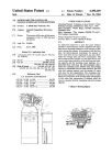
2.1. The Blast Furnace
The blast furnace at Mefos is marked with an A in Figure 2.0.1. A picture of
the actual installation is in Figure 2.1.1. It has three tuyeres and a diameter at the
tuyere level of 1.2 m. The working volume is 8.2
m3 .
The hot blast is produced in
Æ
pebble heaters, capable of supplying 1300 C of blast temperature.
The furnace is
designed for operating with a top pressure of 1.5 bar. It has a bell-type charging
system without movable armour. The coal injection system, see B in Figure 2.0.1,
features individual control of coal ow for each tuyere. Gas cleaning system, part
D of Figure 2.0.1, consists of dust catcher and electrostatic precipitator. Material
is transported to the top of the blast furnace through C as shown in Figure 2.0.1.
A tapping machine with drill and mud gun is installed. The blast furnace is well
equipped with sensors and measuring devices, and an advanced system for process
13
14
2. PROCESS DESCRIPTION
control. Probes for taking material samples from the furnace during operation are
being developed.
Figure 2.1.1. The blast furnace body.
LKAB use the furnace primarily for development of the next generation of blast
furnace pellets.
The furnace performance shows that it is a good tool for other
development projects.
An important area is recycling of waste oxides.
Injection
of waste oxides is another research area as well as injection of slag formers. The
interesting parts of the plant are presented in Figure 2.1.2.
Air Lock Vessel
Blast Furnace
Tuyeres
Slag Vessel
Video
Camera
Coal Injection
Vessel
111111111111111
000000000000000
000000000000000
111111111111111
000000000000000
111111111111111
000000000000000
111111111111111
Figure 2.1.2. The most relevant parts, for this project, of the
experimental blast furnace at Mefos.
2.2. COAL INJECTION
15
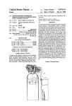
Figure 2.2.1. Control screen for coal injection, at Mefos.
2.2. Coal Injection
The coal injection arrangement, Figure 2.2.1, consists of two coal vessels and
three pipes each ending with a tuyere. The three tuyeres are evenly spaced around
the blast furnace, as shown in Figure 2.2.2.
Pulverized Coal Pipe
Tuyere
Coal Plume
Video Camera
Blast Furnace
Furnace
Wall
Figure 2.2.2. The three tuyeres are surrounding the blast furnace
with the surveillance cameras supporting framework.
Looking again at Figure 2.1.2. The upper vessel, the one that is lled with coal
when needed, works as an airlock vessel used to pressurise the coal vessel below.
From the lower vessel, called the injection vessel, coal is divided and distributed
under pressure through pipes to the tuyeres in the blast furnace with the help of
nitrogen, which serves as a carrier medium. The left vessel is used to inject slag
16
2. PROCESS DESCRIPTION
when desired.
A big problem is determining the behaviour of the coal particles
travelling through the pipes. That is because of the various size of the particles,
turbulence eects in the pipes and pipes' characteristics. Coal particles can clog in
a pipe, which can disturb the process before being discovered. Another problem is
6
leakage of the carrier gas. Solution for the latter is proposed in [ ].
2.3. Current Control
The existing control of the pulverised coal ow to the blast furnace is based on
a continuous on-line measurement of the coal ow itself. Although this is true, it is
not the whole truth. It has been shown that the ow measurement device is not very
accurate, that is why the current control is dependent on a weight measurement of
the injection vessel.
2.3.1. Sensors.
Mainly we can talk about three ow measurement devices,
every one of them connected to pipes transporting pulverised coal to the tuyeres.
The devices used are Ramsey DMK 270 industrial mass ow rate and velocity mea-
16].
suring instruments for non homogeneous media [
Internally the device consists
of a solids concentration sensor and a velocity sensor with two measurement points
separated by a distance
S,
based on the capacitive measuring principle. The par-
ticle stream is measured in two points which the velocity transmitter correlates to
nd the closest similarity between them. From this correlation function, the transit
time
T
from point one to point two can be determined.
In the solid concentra-
tion sensor the change in capacitance is proportional to the solids concentration,
this voltage signal is transformed into a frequency signal and is Pulse Frequency
Modulated (PFM).
Q is given by Q = C V Asensor , where C is the concentration
V its velocity and Asensor is the sensor cross-section area and is
d2
calculated with Asensor = sensor , where dsensor is the sensor diameter.
4
K
The concentration C = 10a (fP F M fP F M0 ) K , where Ka is an adaption factor
to concentration sensor, fP F M is the measured frequency of PFM concentration
signal, fP F M0 is the frequency of PFM signal at concentration zero and K is a
The ow rate
of the medium,
calibration factor. Finally the velocity is calculated with the well known formula
V
= TS .
Not to forget that the both vessels are equipped with weight gauges and pressure
meters. Other important sensors are the pressure measurement devices in the coal
injection pipes.
2.3.2. Controllers.
trollers.
Figure 2.3.1 is a schematic overview of the main con-
Because the owmeter is not reliable, the on-line ow measurement is
multiplied by a correction factor calculated according to the injection vessel weight
loss deviation, during a certain period of time. See Figure 2.3.2 for details. Doing so the idea of on-line measurement is lost, in a short term perspective, while
it is relatively accurate considering a longer period of time.
The corrected ow
measurement itself is the output of a PI-controller using 1 as its setup value and
feedback with the owmeters to coal vessel weight ratio. Before dividing the ow
measurement by the vessel weight both signals are windowed with a window length
of 10 minutes before performing the division. This is done because the scale used
in the vessel has a limited sensitivity and a big error margin, if compared to the
ow measurement during a short time.
The coal injection is controlled with three PID-controllers, one for each tuyere.
An operator is supposed to feed the system with the desired amount of coal ow
needed in the furnace, the amount is divided by three and the result serves as a
setup value for each of the controllers. The output from the PI-controller is used as
2.4. VIDEO SURVEILLANCE
17
Operator
Setup
3
DIV
Coal Injection
Vessel
Flow Meter
kg/s
Valve
Tuyere
DMK 270
x
−
PID
x
−
PID
x
−
PID
Slag Vessel
kg/s
DMK 270
kg/s
DMK 270
1
SUM
WINDOW
DIV
−
PI
XXX
Figure 2.3.1. Coal powder injection control.
Flow Direction
Coal Pipe 1
Concentration
Velocity
.
kg/s
Mass Flow 1
DMK 270
X
Mass Flow 2
Mass Flow 3
Slag Vessel Weight
Coal Vessel Weight
Weight Corrected
Mass Flow 1
Weight Multiplicator
Function
Figure 2.3.2. A principle scheme for pulverised coal mass ow calculation.
feedback. The control signal from each of the PID-controllers is used to control a
valve placed before the owmeter on each pipe. A control based on these terms can
not be perfect having in mind the bad quality of the resulting measured/calculated
signals. Depending on how the multiplicator changes, the control signal will behave
dierently.
We will show later in Chapter 4.1 that some control signals have a
strange behaviour.
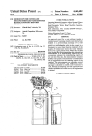
2.4. Video Surveillance
The conditions surrounding the steel making procedure are rather rough. The
very high temperature of the ame and the high brightness from inside the blast
furnace make life hard for those who want to control or study this process. The
existing cameras at Mefos can not handle the incoming high light intensity and they
need to be protected from the heat. A damping lter has to be employed to make
18
2. PROCESS DESCRIPTION
the video picture viewable. The lter itself is a dark green piece of thick glass that
is placed a bit away from the camera lens. The cameras themselves are mounted
about two meters from the outer wall of the blast furnace and are built-in inside a
protecting cover. The light from inside the furnace is led to the cameras through
peek holes in the wall near each tuyere via protecting pipes.
Furnace
Wall
Pulverized Coal Pipe
Protecting Cover
Tuyere
Filter
Panasonic
WV−CL410
Coal Plume
Protecting Pipe
Video Camera
Figure 2.4.1. The video camera setup.
For a full comprehension of the whole video camera apparatus, Figure 2.4.1
might be helpful for the devoured readers. On its way to the lens light passes the
previously mentioned glass lter.
The characteristics of this lter have not been
examined in great detail but having a closer look at the three colour buers shows,
for the human eye, that the red and in particular the green light pass the lter
almost unaected while the blue light is ltered out to the extent that the blue
buer becomes nearly useless, as discussed in Chapter 5. It is therefore desired to
solve the ltering problem. We had the possibility to use transparent glass instead
of the green one, which we believed would leave all the three colour buers unspoilt.
By doing this we risked introducing overexposure to the video surveillance system.
Possible solutions will be discussed later in this report.
(a) With green glass.
(b) With transparent glass.
Figure 2.4.2. Sample images taken with green glass as lter and
with transparent glass.
An example of what is seen with the help of the cameras is in Figure 2.4.2,
where the mouth of the tuyere is seen together with a dark, elliptic shaped cloud,
the pulverised coal injected inside the furnace.
CHAPTER 3
Collecting Data
Doing a project of this nature needs of course collaboration with the industry in
order to improve things. Simply there is a need of being at the eld for investigating
possible ways to get across suitable data to kick-o the project. People working at
the plant know how to run it and how it behaves. Collecting data does not only
mean pure data measurements, it also includes collecting the knowledge possessed
by the plant workers. Every detail is important, every worker has something to tell
that we probably need to know. The knowledge we gained from people in the eld
is spread all over the report. Below we are dealing mostly with measurement data
collection.
3.1. Available Signals and Equipment
To start with, we will shortly discuss which signals were available to us for further study. After an exhaustive investigation of the process and the parameters that
were available and examining the signal collecting equipment we nally concluded
what had to be done. It was obvious right from the start that the coal ow signals
were of importance for this project. Also the nitrogen pressure in the pipes leading
the pulverised coal to the blast furnace was thought to be of interest. Further some
other signals were considered in case they would later show to be signicant for the
study of the coal powder ow.
For convenience Table 1 with available signals is
attached. Of course there were many other signals available but we did not think
that they were of interest.
Nr.
Connection
Internal Signal Tag
Signal Description
Range
1
205
31PI101
Pressure, inj. pipe 1
0-16 bar
2
207
31PI102
Pressure, inj. pipe 2
0-16 bar
3
209
31PI103
Pressure, inj. pipe 3
0-16 bar
4
298
31FV138
Control sig., pipe 1
0-100%
5
300
31FV139
Control sig., pipe 2
0-100%
6
302
31FV140
Control sig., pipe 3
0-100%
7
029
31FI101
Mass ow, pipe 1
0-41667 g/s
8
031
31FI102
Mass ow, pipe 2
0-41667 g/s
9
033
31FI103
Mass ow, pipe 3
0-41667 g/s
10
237
31PI021
Pressure, inj. vessel
0-20 bar
11
470
31WI001
Weight, inj. vessel
0-3000 kg
12
322
31PI108
Pressure, lock vessel
0-16 bar
13
474
31WI102
Weight, lock vessel
0-3000 kg
Table 1. The considered signals and their description.
Unfortunately the collected signals could not be taken straight from Mefos'
computer system.
The reason for this was simply the decient capacity of the
presently used system.
In this case it was necessary to wire a signal collecting
19
20
3. COLLECTING DATA
equipment into an electrical cabinet, consisting of a National Instrument data acquisition box SCXI-2000 equipped with SCXI-1120, an 8-channel isolation amplier
and SCXI-1100, a 32 channels programmable amplier with gains. Those modules
contained an IO-board and an analogue to digital converter with ampliers. In total we had two dierent opportunities to log signals, we did that on three dierent
dates. The 8-channel card was used in the third logging session while the other one
was what we had in the rst and second session. A portable computer was used to
store data with the help of the data collecting programme LabView. This was the
best option available although not very favourable, which will be discussed later.
The signals in the electrical cabinet were in the range of 4-20 mA, a current circuit
connection was employed for its robustness to signal noise, not aecting the plant
and its easiness.
Not surprisingly this project also demanded video recordings from the three
cameras, beside the previously mentioned signals.
These video signals could be
found at another electrical cabinet at the plant. Using ordinary video recorders,
video signals could be recorded for later usage and investigation.
3.2. Measured Signals
Knowing the situation presented in the previous section and the uncertainty of
which signals to collect, a decision was made to collect all of the 13 listed signals
considered if possible. This was done during the rst data gathering on the 4th of
June 1999. Although some problems arose in the blast furnace, data was stored
on a laptop and transferred to stationary computers standing in a small image
processing lab at Luleå University of Technology, for later consideration. A couple
of days later sadly the pressure signal of injection pipe 1 was discovered to be faulty.
It was necessary to arrange another signal collecting session, which was eventually
done on the 10th of June 1999. This time all signals were ne except for one of the
video signals. Apparently we can not have them all! Again there were problems
with the furnace process during data gathering time, which later turned out to
possibly be related to the equipment used. Although the data acquisition module
was thought to be galvanically isolated. Unfortunately it was found that was not
the case.
Neglecting that fact collected data was analysed.
logging sessions we used the same cabling with 250
During both those
resistances.
Wanting to verify what was concluded from the data collected in June another
trip to Mefos was required. This time, not wanting to be be blamed for disturbing
the blast furnace process once again.
used.
Another data acquisition card had to be
The National Instruments signal collecting box turned out to have a card
supporting collection of only eight signals at a time, if they were to be isolated. We
also changed the cables used and switched to 50
resistances.
This was found to
be a good solution after an examination of what went wrong with the blast furnace
process during the June sessions at Mefos. Of course, a limitation like this meant
a risk. An omitted signal could later turn out to be of great importance. We had
to concentrate on two of the three tuyeres, specically pipe 2 and 3. The chosen
signals have, looking in Table 1, numbers 2, 3, 5, 6, 8, 9, 10 and 11. Motivation for
this choice was that mass ow was wanted together with both the control signal
and pressure signal. Weight of the injection vessel as well as the pressure inside it
were also taken into consideration on the expense of the control, pressure and ow
signals for tuyere 1. Control, pressure and ow signals in pipes 2 and 3 were thought
to be sucient regarding the small number of signals that could be gathered using
the available equipment.
The main reason for this logging session was to record
a new video signal of the injection without using a green glass lter, instead we
changed the glass in front of the camera in pipe 2 to a transparent one. The glass
3.2. MEASURED SIGNALS
21
in front of the other camera, pipe 3, remained unchanged. Bad luck and possible
wiring problems resulted in a missed signal, this time it was the coal injection vessel
weight. A summary list can be found in Table 2. Other activities at the plant linked
to our work can be found in Table 3.
Occasion
Date
Time Duration
Collected Signals
Tuyeres Recorded
1
999-06-04
17:54:08-18:47:23
2-13
1, 2, 3
2
999-06-10
12:45:46-14:49:08
1-13
1, 2
3
999-11-18
13:24:34-15:04:24
2, 3, 5, 6, 8, 9, 10
2, 3
Table 2. Data collection occasions.
Occasion
Slag
1
g Nm3
h
Coal Setup Value
kg
h
i
Tapping Time
No
130
18:47-18:51
2
20
125
3:04-13:19 14:30-14:36
3
No
125
14:05-14:15
Table 3. Activities and setup values during the logging time.
During the third logging session we had an opportunity to disturb the coal ow
in one of the pipes. We chose pipe 2. This test series originated from a need of
data for an extra validation of achieved results in a dierent project ran by Ph.
D. student Andreas Johansson related to his research in clogging detection in a
6
pressurised system [ ] at Luleå University of Technology.
series as Andreas test.
We refer to this test
This test is also interesting in our case to see if we can
detect the ow changes with image processing. We had two valves which we could
close to prevent the coal ow into the furnace. The rst valve was located directly
after the injection vessel and before the owmeter, the other valve was placed after
the owmeter; we refer to those as the valve before and the valve after, relative
to the owmeter as illustrated in Figure 3.2.1. We opened and closed the valves
repeatedly with dierent throughput rates. The test duration was limited due to
a desire for not aecting the plant or ending up with a plugged pipe. We realised
later that the time between the dierent actions was not far from the limit of being
too short, because the ow measurement is very strongly ltered; see Chapter 4.1
for further insight.
Coal Injection
Vessel
Slag Vessel
Controlled
Valve
Flow Meter
kg/s
Valve
After
Tuyere
DMK 270
Valve
Before
Figure 3.2.1. The locations of valves along the injection pipe.
Table 4 shows the actions taken during the test, the valve position we mention
is actually the valve handle position and not the real valve opening rate (position)
22
3. COLLECTING DATA
which is most likely non-linear. Notice that the valves were totally opened before
and after the test.
Other signals as slag vessel weight and its pressure as well
as weight correction multiplicator should have been collected, but this was not
discovered before it was too late.
Action
Time
Valve placement
1
14:23:30
after
Valve position
1/2 closed
2
14:24:30
after
1/1 opened
3
14:26:00
after
1/1 closed
4
14:27:00
after
1/2 closed
5
14:27:30
after
1/1 opened
6
14:29:00
after
1/2 closed
7
14:31:40
after
1/1 closed
8
14:33:00
after
1/1 opened
1/2 closed
9
14:36:00
before
10
14:36:30
before
1/1 closed
11
14:37:30
before
1/1 opened
12
14:38:00
before
1/2 closed
13
14:39:00
before
3/4 closed
14
14:39:40
before
1/1 closed
15
14:41:00
before
1/1 opened
Table 4. Actions and time schedule during Andreas test.
3.3. Video Recording
At the same time as data was collected using the data collecting module a video
recording had to be made. This was clearly a sensitive issue to deal with. The time
delay between the start of collecting other data and recording the video signals from
the cameras had to be determined in some way, because those signals were to be
compared during later analysis. The only viable alternative was to start gathering
data at a certain point in time, then start the video recording and marking a xed
point in time on the lm sequence by manually dimming the light to the cameras
for a couple of seconds. That way the time delay was restored later when analysing
data. Using a more sophisticated synchronisation method would be a better option
if it was not such a lengthy procedure, remembering that the electrical cabinets and
the cameras are apart from each other making a complex wiring scheme doomed to
fail in such environment, and also having in mind the quite small benets employing
an approach dierent from the simple solution used.
Video cameras presently installed at Mefos are of the type Panasonic WV-CL
410. These cameras were used at both occasions in June. However in November a
decision was made to try another, slightly more advanced camera for lming the
injection at tuyere 2.
The camera used was also a Panasonic camera from the
400 series. The dierence was mainly the larger dynamic range, and employment
of a new Panasonic technique known as SuperDynamic. Good reference manuals
with the camera specications could not be found. The necessity of using a more
advanced camera occurred to us when trying to record a lm sequence without
the dark green protecting glass. Operators knew from experience that the existing
cameras were not able to handle the intake of very bright light when the protecting
glass was removed. Removing the dimming lter, transparent glass was mounted
in its place.
The new camera used was performing better than the old one but
3.4. VIDEO DIGITISING
23
unfortunately it also reached the saturation point due to the extreme brightness of
the light from inside the blast furnace.
Another problem discovered during the signal collecting session in November
was the dynamic adjustment of the range. This caused changes in the background of
the picture depending on the amount of visible coal. When there is a lot of coal the
picture is percepted as darker by the camera so it adjusts to a darker picture, when
there is no coal the picture is brighter and again the camera adjusts accordingly.
As a result of these constant adjustments we get a background for the pulverised
coal cloud that is constantly changing.
Those changes are not great but can be
irksome when, for instance, trying to retrieve information about the temperature
of the ame. Problems are in that case caused by the fact that a change in colour
does not have to reect a change in temperature, which seems like a troublesome
case to solve. Maybe the easiest way to deal with this problem would be disabling
the auto adjustment function in the cameras used.
Further another source of concern is the noise introduced by the poor quality
video tapes and the video recorders themselves. Watching a recorded sequence it is
apparent for a human observer that unwanted noise is present. Luckily the extent
of this phenomenon is limited and it should not aect the outcome of later analysis
too much.
All problems discussed are evidently of harm for the quality of images to be
analysed. Obviously a higher quality of images is better but it has to be pointed
out that their quality is still well above what is needed for image processing to be
performed in order to obtain vital information about the blast furnace process.
3.4. Video Digitising
The recorded video signals on the tapes needed to be converted into a usable
format in order to process them in a computer.
Digitising the video signals was
required. It is always hard to choose a computer environment to work with, in our
case the choice was easy. Microsoft's Windows family has never been a choice of a
serious researcher/engineer and hopefully will never be, specially when she/he deals
with automatic control. Free Software is widely available, reliable, supported and
sucient in most cases. We used RTLinux as a platform for digitising the video
tapes we recorded.
Using an ordinary S-VHS video player, a common PC (old
timer) equipped with RTLinux, a Matrox Meteor frame grabber card and a simple
grabbing program, see the source code in Appendix B.1, the work was accomplished.
The task here is to convert a full motion video, PAL-signal (Phase Alteration
Line) running at 25 frames per second, into single frames stored in a digital format.
The rst step in the process of converting an analogue signal into a digital representation is sampling. This is accomplished by measuring the value of the analogue
signal at regular intervals called samples. These values are then encoded to provide
a digital representation of the analogue signal. The power spectral density (PSD)
of the ow signals, we have collected, shows that in the worst case a sampling time
of two seconds is sucient. Remember that we are not sampling to control, we are
just trying to recreate the ow signal in someway. Two seconds might sound too
fast but some of our ow signals have a signicant frequency peak caused by bad
control. The same frequency peak has been found in the pressure and control signals. See Figure 4.1.3 for a closer look at PSD signals related to pipe 2, taken form
the second data collecting occasion, which can be compared to the ones related to
pipe 1, also from the second occasion, in Figure 4.1.4. As you can see the peaks
in (a), (b) and (c) are below 0,2 Hz, which means according to Nyquist's sampling
theorem, that a sampling time of 2,5 seconds (
1
) should be sucient. Choosing
0;2 2
24
3. COLLECTING DATA
3 seconds sampling time is kind of adventurous because it will catch up with frequencies up to 0,16 Hz which may result in some aliasing in our case. We assumed
that the characteristics, in the collected signals, would be reected in the data to
be extracted from the recorded video signal. Actually the ow measurement device
used a couple of seconds data ltering and the control system used at Mefos use a
time base of 0,20 - 0,25 seconds.
(a) 10 frames before capturing.
(b) 10 captured elds of the frames above.
3
Figure 3.4.1. Interlace principle [ ].
Video is sampled and displayed such that only half the lines needed to create
a picture are scanned at a particular instant in time. A video frame in our case
consists of two interlaced elds of 625 lines. Interlace is the manner in which a video
picture is composed, scanning alternate lines to produce one eld, approximately
every 1/50 of a second in PAL. Two elds comprise one video frame.
As shown
in Figure 3.4.1, if the upper sequence is captured by a conventional video camera
the result will be the lower sequence which means that our frame consists of two
dierent elds captured at dierent times. This is a drawback in digitising analogue
video signals that use interlace. We had to separate each captured frame into two
elds, but this did not aect our results. A reason for that is: We sampled at a
very low rate compared to the eld rate and it is not very likely that much of the
image, in our case, has changed in 1/50 seconds. Figure 3.4.2 shows how this eect
is present in our case.
Another important factor when it comes to digitising is the frame grabber
equipment. The used frame grabber card, a PCI Matrox Meteor, should be considered as appropriate in our case. The card could make 24 bpp at
resolution. This gave us
256 256 256 (RGB) colours.
768 576 pixels
At the time this project
started the device driver available for the grabber card, for Linux, was not of a
very high quality. We were forced, due to some possible hardware limitations, to
increase the delay time for the card in order to make the desired resolution mentioned above.
This could sometimes lead to unwanted eects, which resulted in
grabbing an image combined of two frames, see Figure 3.4.3. We had to accept this
bug for the time being, specially because it does not appear so often and could not
have a major inuence on the total result.
We did not use the real-time functionality in RTLinux for several reasons: The
program we wrote for grabbing the video frames gave a good synchronisation (a
3.4. VIDEO DIGITISING
25
Figure 3.4.2. Interlace phenomenon in a sampled frame, from
our video recording.
Figure 3.4.3. An image composed of two dierent frames.
couple of milliseconds), the sampling time was 2 seconds so a strict time scheduling
was not necessary and we wanted to make the program code for grabbing the frames
easier. Bear in mind the data acquisition programme used, LabView, was running
on Windows 95 sampling data every second. We have every reason to assume that
the sampling was not perfect on the millisecond level.
Because lack of a very good synchronisation signal, as mentioned in Chapter
3.3, to start grabbing the images we had to rely on our extremely good reex time
26
3. COLLECTING DATA
and start grabbing when the synchronisation signal was visible on a monitor screen
attached to our VCR. Any mistakes here will result in a time delay when comparing
the logged data with the one extracted from the sampled video recording, which is
hopefully much smaller than the overall time delay for the whole system.
A fully operational system based on real-time image processing of the video
signal should consider to deal with a short sampling time and enjoy using the real
time features in RTLinux.
CHAPTER 4
Data Processing
The collected data is of no use if it is not analysed with a critical eye. Knowing
the data characteristics and its limitations is of great help when it is later used
in Chapter 7 for validating the extracted ow measurement. Decisions based on
the analysed data can then be taken with good accuracy. To make this analysis
fast and practical, a small user interface was written in MATLAB. It was given the
name Danalyzer from the two words "data" and "analyse" and will be described
later in Chapter 4.2.
4.1. Analysis of Signals
Performing the analysis of collected signals it is close at hand to start by looking
at the plain signals, comparing their shapes and trends. Trying to nd possible similarities which could reveal interconnections and dependencies between the signals
is basically the rst step.
To start with the pressure signals were viewed. First signal collecting occasion
gave us only the last twelve signals according to their numbers in Table 1.
As
mentioned before the pressure in injection pipe 1 was not stored due to hardware
problems. The other two pressure signals looked quite the same, the pressure in
injection pipe 3 being slightly higher than the pressure in injection pipe 2. We do not
think that should be the case. The level, not considering the fast uctuations, was
quite constant. Then the mass ow for the three pipes was examined. It seemed to
be almost the same in all pipes although of course small dierences could be noticed.
Moving over to the control signals it could be noticed that the control signal for
pipe 1 was behaving in a much better way than control signals for pipes 2 and
3. Looking at those signals it is clear that the controllers are not working as they
should. Both the control signals 2 and 3 reach their lower bound frequently and are
varying quite a lot which indicates bad control. Well, with a risk of being nasty we
would say, very bad control. Examine Figure 4.1.1 for clarication. Could this be
a result of our non-galvanically isolated data acquisition equipment? A comparison
between the control signals from the rst and the second data collecting occasions,
which we carried out using the same cabling, shows that the control signals do not
saturate as often as the one in Figure 4.1.1 does. This makes us conclude that we
are not responsible for the bad control, something else went haywire. The controller
for pipe 1 functions somewhat better at that given time. Pressure as well as weight
of the lock vessel remain constant for the whole time period.
For the injection
vessel pressure we notice a sinusoidal looking curve with a diminishing amplitude,
whereas its weight is steadily falling because coal powder is persistently drawn from
it and transferred to the blast furnace and no rellment of the coal vessel has taken
place during logging time. The constant negative slope of the signal suggests an
even supply of coal to the blast furnace.
The second time we went to Mefos to collect signals we managed to get all
thirteen of them i.e. the same twelve as before and also the pressure in injection
pipe 1. Pressure signals for the three pipes look very much the same and there is
nothing distinctive about them except for the sudden variations seen throughout a
27
28
4. DATA PROCESSING
A plain plot for [31FV139]
2.4
3
2.3
2.8
2.2
2.6
2.1
Sensor value
Sensor value
A plain plot for [31FV138]
3.2
2.4
2.2
2
1.9
2
1.8
1.8
1.7
1.6
1.6
1.4
0
500
1000
1500
2000
2500
3000
3500
Sample
1.5
0
500
1000
1500
2000
2500
3000
3500
Sample
(a) Pipe 1.
(b) Pipe 2.
A plain plot for [31FV140]
2.3
2.2
2.1
Sensor value
2
1.9
1.8
1.7
1.6
1.5
0
500
1000
1500
2000
2500
3000
3500
Sample
(c) Pipe 3.
Figure 4.1.1. Control signals, rst data logging occasion. X-axis
is samples taken 1 per second and Y-axis is sensor value in Volts.
section in the rst part of the data. This is not as obvious in the mass ow signals
except for the ow signal for pipe 3. Actually it is hard to tell anything decisive
studying the mass ow in pipes 2 and 3. Possibly the ow is slightly higher in the
rst part of the data. The control signals are weird looking things which have very
little in common. Control signal for pipe 1 is following a constant line with quick,
high variations. In control signal 2 we can discern that the signal drops after a while
which resembles a little the behaviour of control signal 3. In the last mentioned
signal again clear deviation from normal behaviour appears in the beginning. Lastly
looking at the injection vessel and air lock vessel signals it is clear that something
happens exactly the same time as seen in the other signals.
The strange behaviour in the beginning has been shown to be caused by tapping
of iron during logging time as stated in Table 3. Although the time does not exactly
match there is no indication that it could be caused by anything else.
The rst
tapping is visible in all the signals but the second one appears only in the control
signal of pipe 2. It has nothing to do with the duration of the tapping, because the
eect on the signals is visible during the whole tapping time. What happens in the
blast furnace during the tapping is a very interesting topic to look into.
4.1. ANALYSIS OF SIGNALS
Test signal and [31FI102], detrended with the sample means removed
29
A dtrended plot for [31PI102] with the sample means removed
1.5
0.04
1
0.03
0.5
0.02
Sensor value
Sensor value
0
−0.5
−1
0.01
0
−1.5
−0.01
−2
−0.02
−2.5
−3
3200
3400
3600
3800
4000
4200
Sample
4400
4600
4800
5000
5200
(a) Flow signal, compared to valve position.
3600
3800
4000
4200
Sample
4400
4600
(b) Pressure signal, compared to valve
position.
A dtrended plot for [TEST005] with the sample means removed
3
2
Sensor value
1
0
−1
−2
−3
3200
3400
3600
3800
4000
4200
Sample
4400
4600
4800
5000
5200
(c) Control signal, compared to valve position.
Figure 4.1.2. Measured signals in pipe 2 (blue) compared to valve
position (red) during Andreas test. X-axis is samples taken 1 per
second and Y-axis is sensor value in Volts.
During the November visit to Mefos only eight signals were collected due to the
previously mentioned hardware limitations. One of these signals turned out to be
of no use, namely the injection vessel weight signal. Pressure in the vessel seems to
be relatively constant. Now looking at the other signals we have to keep in mind
that we choked the pulverised coal ow for injection pipe 2 in Andreas test, as we
mentioned in Chapter 3.2. Strangling the ow could only be done for short periods
of time not to block pipe 2 permanently, needing a serious intervention in the
system. Not very surprisingly inspecting the ow signal 2 we can unambiguously
see distinct changes in the ow, as Figure 4.1.2-(a) clearly shows. A very interesting
thing is the delay in the ow measurement signal, it seems to be caused by some
lter; this made us start scratching our heads. Later, this discovery will be treated
in Chapter 4.1.1.
Another interesting observation is that the ow is not really aected until a
valve is totally opened or totally closed and we have an overshoot when a valve is
totally opened. A possible reason is that the valves have a non-linear characteristics
and that, as shown below, the ow can be kept as long as the pressure is constant.
30
4. DATA PROCESSING
A shame is that we never let the ow measurement settle or saturate before we
changed the valve position. The pressure signal in pipe 2 did also respond to our
test, strangling of the pipe reveals itself by an increment/decrement in pressure.
As shown in Figure 4.1.2-(b) the pressure increases each time the valve after the
owmeter is closed and decreases each time the valve before the owmeter is closed.
It seems that the pressure in the pipe can be kept constant when a valve is half
closed.
The PSD for [31FI102] decimated2 times
The PSD for [31FV139] decimated2 times
40
40
30
30
Power Spectrum Magnitude (dB)
Power Spectrum Magnitude (dB)
20
10
0
−10
20
10
0
−10
−20
−20
−30
−40
0
0.05
0.1
0.15
0.2
0.25
−30
0
Frequency
0.05
0.1
0.15
0.2
0.25
Frequency
(a) Mass ow.
(b) Control.
The PSD for [31PI102] decimated2 times
30
20
Power Spectrum Magnitude (dB)
10
0
−10
−20
−30
−40
−50
0
0.05
0.1
0.15
0.2
0.25
Frequency
(c) Pressure.
Figure 4.1.3. PSD plots for dierent measurements in pipe 2,
second occasion. Frequency is in Hz.
good look at the control signal of pipe 2, presented in Figure 4.1.2-(c) ensures
us about a reaction from the controller. The response time is about 30 seconds.
Sometimes we were about to reopen the valve before the controller hits its upper
limit.
The more important thing is that the control signal increases when the
valve is closed, which is an indication of a functioning controller. The controller's
feedback, see Chapter 2.3 for further information, is a reason for the bad response
time; unless Mefos' engineers have designed it that way. That proves that at least
there is a reaction from the owmeter when the coal ow to the furnace is drastically
reduced. What can be considered as strange is that looking at the pressure, control
and ow signals for pipe 3 there are no changes that could be directly connected to
the changes in the ow for pipe 2. Since the coal leaves the injection vessel and is
4.1. ANALYSIS OF SIGNALS
31
then divided in three ows one could conclude that smaller ow in one of the pipes
would mean more coal in the remaining pipes if the total ow was to be the same.
Here we can deduce that either the total ow decreased or that the owmeters do
not work very well.
The PSD for [31FV138] decimated2 times
40
30
30
20
20
Power Spectrum Magnitude (dB)
Power Spectrum Magnitude (dB)
The PSD for [31FI101] decimated2 times
40
10
0
−10
10
0
−10
−20
−20
−30
−30
−40
0
0.05
0.1
0.15
0.2
0.25
−40
0
Frequency
0.05
0.1
0.15
0.2
0.25
Frequency
(a) Mass ow.
(b) Control.
The PSD for [31PI101] decimated2 times
30
20
Power Spectrum Magnitude (dB)
10
0
−10
−20
−30
−40
−50
0
0.05
0.1
0.15
0.2
0.25
Frequency
(c) Pressure.
Figure 4.1.4.
PSD plots for dierent measurements in pipe 1,
second occasion. Frequency is in Hz.
Next step in the study of the collected signals was to try dierent things, like
for example addition, subtraction and other such operation on the dierent signals.
One of the more interesting things tried here was frequency analysis. Frequency
contents of our signals were analysed using Danalyzer, just as all of the above
analysis to make life simpler and save some time. Studying signals collected on the
4th of June, we found the same dominant frequency for pipe 2 and 3 in control and
ow signals, as shown in Figure 4.1.3 for pipe 2. This could point to poor control
aecting the ow and making it uctuate or the opposite, if we assume that the
controllers are the same in all the pipes but the ow measurement device behaves
badly in dierent ways. For our purposes though this was an excellent opportunity
to check if the same frequency could be found in the processed images. This matter
will be investigated in Chapter 7.2, where all the data extraction is performed and
thoroughly discussed. We could not identify such control problems for pipe 1, see
32
4. DATA PROCESSING
Figure 4.1.4, nor could they be found in the signals collected later, which should
not be misinterpreted as the control signal being unsurpassed.
1
1
3 sec.
0.8
0.8
3 sec.
0.6
Correlation coefficient
Correlation coefficient
0.6
0.4
0.2
0.4
0.2
0
0
−0.2
−0.2
−0.4
−500
−400
−300
−200
−100
0
100
Time shift [seconds]
200
300
400
−0.4
−500
500
(a) Control-pressure, rst logging.
−400
−300
−200
−100
0
100
Time shift [seconds]
200
300
400
500
(b) Control-pressure, third logging.
0.4
0.8
24 sec.
0.3
25 sec.
0.6
0.2
0.4
0.1
Correlation coefficient
Correlation coefficient
0.2
0
−0.1
−0.2
0
−0.2
−0.4
−0.3
−0.6
−0.4
−0.8
1 sec.
−0.5
−2 sec.
−0.6
−500
−400
−300
−200
−100
0
100
Time shift [seconds]
200
300
400
−1
−500
500
(c) Control-ow, rst logging.
−400
−300
−200
−100
0
100
Time shift [seconds]
200
300
400
500
400
500
(d) Control-ow, third logging.
0.4
0.6
23 sec.
0.3
260 sec.
0.4
0.2
0.2
Correlation coefficient
Correlation coefficient
0.1
0
−0.1
−0.2
−0.3
0
−0.2
−0.4
−0.4
−0.6
−0.5
−4 sec.
−1 sec.
−0.6
−500
−400
−300
−200
−100
0
100
Time shift [seconds]
200
300
(e) Pressure-ow, rst logging.
400
500
−0.8
−500
−400
−300
−200
−100
0
100
Time shift [seconds]
200
300
(f) Pressure-ow, third logging.
Figure 4.1.5. Correlation between pressure, ow and control sig-
nals for the rst and third collected data.
4.1. ANALYSIS OF SIGNALS
33
By looking at the correlation between dierent signals, we can see how hard they
are coupled and see if there exist any delays. Figure 4.1.5 shows clear correlation
between the control and pressure signals. The control signal does not follow the ow
signal as well as the pressure does. This indicates that either the control is bad or
there is something else beside the ow signal that aects the control signal (which
we will see is true here) or both. Almost the same correlation is found between the
pressure and the ow signals. The same gure shows delays between the dierent
signals. Notice that the the correlation plots are dierent if you compare those from
the rst nd the last occasion, there is a clear frequency present in the Figure 4.1.5(a) , (c) and (e). It is most likely the frequency we have pointed out earlier, that
we call Mefos carrier-frequency. Beside the dierence in the frequency the delays
seem to be pretty much the same in both the rst and third data collection. The
pressure is very dependent on the control signal with a delay of 3 seconds. In the
control-ow correlation we see the clear feedback eect, represented as a negative
correlation with a very short delay and the positive correlation with a ow signal
following the control signal after a delay of about 25 seconds. Notice also that the
negative correlation in the third signal logging is much stronger than the one in the
rst one, implying a stronger feedback coupling. The pressure-ow correlation plots
are very much alike the control-ow correlation plots, with almost the same delays
translated by about -2 seconds which conrms what we saw in the control-pressure
and control-ow plots.
Having just these signals to study, it is hard to draw further conclusions. They
were mainly collected in order to, at a later stage, be compared to data extracted
from recorded lm sequences. Thus, just as means to verify our sequitures from
image processing of the video.
Flow signal in pipe 2, before and after filtering
Flow signal in pipe 2, before and after filtering compared to valve position
5
4
4.5
4
3
Measurement [Volt]
Measurement [Volt]
3.5
2.5
2
3.5
3
2.5
2
1.5
1.5
1
1
500
1000
1500
2000
2500
3000
3500
Samples [1/second]
4000
4500
5000
5500
(a) Filtered and unltered signal.
Figure
3400
3600
3800
4000
4200
4400
Samples [1/second]
4600
4800
(b) Filtered, unltered and valve position
signals.
4.1.6. Comparison
between
the
ltered
ow
signal
(green), unltered ow signal (blue) and the valve position signal
(red).
4.1.1. Filter Identication.
We saw earlier that the ow measurement did
not respond in the way we expected it to do when applying Andreas test. Because
we had no access to documentation regarding the owmeter and the control system
in general, at the time we ran into this, we started to investigate the case.
lter was a good way to start in.
A
Connecting a lter to a measurement device
34
4. DATA PROCESSING
is quite common.
A possible lter could be:
H (z )
identication.
= z(1
1
e 22:3679 )
,
1
z e 22:3679
obtained by
Inverting the lter and ltering the ow measurement with it should hopefully
recreate the supposed original signal. Figure 4.1.6-(a) hows how the ltered signal
is related to the original signal and Figure 4.1.6-(b) shows how this ts with the
valve position, after zooming on the interesting parts. A further knowledge of the
control system has shown that, as mentioned in Chapter 2.3, the feedback signal
sent to the controller is not the pure ow measurement we have examined here.
Having a look in the user manual for the owmeter the lters are integrated in
the sub-measurement used in the device in order to calculate the ow.
For our
knowledge the measurement device can not be separated into a ow measurement
and a lter.
4.2. Danalyzer
Figure 4.2.1. A screenshot of Danalyzer.
A tool to simplify the routine work in MATLAB had to be developed.
1
found a tool called Danalyzer
4
We
that was developed during another project [ ] at
Luleå University of Technology.
Danalyzer was in its early development stage,
version 0,1, and needed some work to make it suitable for our needs. After further
development we reached what we called version 0,2. A screenshot is in Figure 4.2.1.
The Danalyzer essence is its portability and the ability to use for dierent purposes
whenever there are signals involved that need to be analysed.
Danalyzer should
combine ease of use with functionality and eliminate the tedious work to produce
needed plots and perform data analysis.
Danalyzer today is capable of viewing and manipulating data in dierent ways,
the main features are:
Viewing of signals.
Browsing through the signals to view specic parts of them.
Several plots on one window.
Multiple windows with dierent plots simultaneously.
Analysis: FFT, PSD, removal of trends.
Adding and subtracting signals.
Decimation of the signals.
Simplicity in creating data les.
Possibility of zooming and gridding.
Loading of signal sets.
1 Dnalyzer
les, version 0,1. URL: http://mir.campus.luth.se/washers/work/danalyzer/
CHAPTER 5
Image Processing
In order to be able to evoke any useful information from the images we have
sampled, we need to know more about them.
A need for a close examination
of the images general properties is as important as the images themselves.
As
we mentioned before we used two dierent types of glass as lters during the video
recording. We also used two dierent types of cameras. This makes the comparison
we made here below not as bulletproof as we wanted it to be.
We will strive to explain most of the image processing carried out by inserting
nice illustrative images and plots as a complement to the explanatory text. In the
very beginning it might be appropriate to explain two systems for representation
of colour images, RGB and HSI. Later we will try to visualise the image content
using dierent techniques.
5.1. Image Decomposition
Any description of the human visual system only serves to illustrate how far
computer vision has to go before it approaches human ability. In terms of image
acquisition, the eye is totally superior to any camera system yet developed. People
are continuously trying to improve the existing articial vision systems.
One of
the problems to be solved is how to represent colours. Several systems have been
invented for this purpose. Here we will only discuss a couple of the most frequently
used systems, RGB and HSI.
5.1.1. RGB and HSI spaces.
First the RGB system will be presented. RGB
stands for red-green-blue. Using these three colours in dierent amounts almost any
other colour can be produced. On a screen mixing is done by having three adjacent
dots, one dot for each of the three colours. If these dots are small enough and the
observer is far enough away, this gives the appearance of one pixel colour rather
than three adjacent ones.
These three colours are primary colours, mixing any
combination of two of them does not make the third.
could be used, providing they are independent i.e.
In fact any three colours
primary.
RGB is the most
widely spread colour system.
HSI stands for hue-saturation-intensity.
HSI may be regarded as the same
space as RGB but represented in a dierent coordinate system. Hue is eectively
a measure of the wavelength of the main colour i.e.
representing dierent colours.
E.g.
there are dierent numbers
lets say 0 represents red, then move all the
way through dierent colours up to 256, in case we have 256 colours, which again
represents red. Imagine a coloured disc that warps around, here 256 is mapped to 0.
Saturation is a measure of hue in each spot. If saturation is 0, then the nal colour
is without hue, i.e. it consists of white light only. Intensity is simply a measure of
brightness of each pixel.
Consult Figure 5.1.1 for a visualisation of the colour spaces.
5.1.2. Image Quality.
Colour image capture involves the capture of three
images simultaneously. With RGB, an early industry standard, intensity of each of
red, green and blue has to be measured for each spot. These are then stored in three
35
36
5. IMAGE PROCESSING
(a) RGB model.
(b) HSI model.
7
Figure 5.1.1. RGB and HSI model representation [ ].
(a) Full color.
(b) Red component.
(c) Green component.
(d) Blue component.
(e) Grey scale.
(f) Hue component.
(g)
Saturation
component.
(h)
Intensity
component.
Figure 5.1.2. An image example with its decompositions in RGB,
HSI and grey scale.
matrices, every matrix containing the values for one of the colours. In our case every
spot in a matrix holds a value representing the intensity of the particular colour.
For each spot in every of the three matrices we had eight bits available allowing
256 dierent values between 0 and 255, where 0 represents the lowest intensity and
255 the highest. Using MATLAB the grabbed images could be transformed into
5.1. IMAGE DECOMPOSITION
this form.
37
Now further operations could be applied to them in order to retrieve
vital information. MATLAB allows also a transition from RGB to HSI and further
manipulation of images.
As an example a nice picture taken outside Luleå University of Technology
representing the university's logotype engraved in a block of ice, Figure 5.1.2, has
been separated into its RGB-components. We can also see the same image in grey
scale and its HSI-components. Dissection performed on this image will be used for
a quick comparison to our grabbed images.
(a) Full color.
(b) Red component.
(c) Green component.
(d) Blue component.
(e) Grey scale.
(f) Hue component.
(g)
Saturation
component.
(h)
Intensity
component.
Figure 5.1.3. An image taken with a green glass, with its decom-
positions in RGB, HSI and grey scale.
Now, decomposing an arbitrary image from inside the blast furnace taken with a
green glass in front of the camera gives images in Figure 5.1.3. For RGB, the red and
green part look ne whereas the blue one looks dierent due to the characteristics of
the lter. For HSI, the hue and saturation buers are very noisy and therefore hard
to deal with. The intensity component is quite alright though. Hue and saturation
can be compared to the ones in Figure 5.1.2 where no noise is present.
Finally the same was done to an arbitrary chosen image from the lm sequence
lmed with a transparent glass, Figure 5.1.4. Blue component of the RGB looks
better here than in the previous series.
It would therefore be advantageous to
use transparent glass. Evidently, being able to use three channels instead of two
would increase the redundancy when approximating the pulverised coal ow.
A
restriction here are the cameras used. The very bright light makes even the better
cameras saturate. That is clear in the saturation component in Figure 5.1.3, the
lower area of the interior of the blast furnace, and in Figure 5.1.4 it is visible on
the edges around the peek hole.
Fortunately, strictly measuring the ow should
not be aected too much by cameras saturating for pixels surrounding the plume.
Temperature measurements of the ame would be much more problematic. Looking
into the hue, saturation and intensity buers we can conclude that there is still
noise present for hue and saturation although it looks sharper than previously. The
intensity component is not remarkably aected, it look more alike the grey scale
image than it did in the image taken with green glass.
38
5. IMAGE PROCESSING
(a) Full color.
(b) Red component.
(c) Green component.
(d) Blue component.
(e) Grey scale.
(f) Hue component.
(g)
Saturation
component.
(h)
Intensity
component.
Figure 5.1.4. An image taken with a transparent glass, with its
decompositions in RGB, HSI and grey scale.
5.2. Image Content
An important issue is to nd the dierence between a coal free image and
another one with coal. A coal free image does not mean a gas free image, nor does
it mean an activity free image. It is only an image that seems to have less coal
than other images in general. This dierences might be viewable when looking at
the intensity histograms of the picture. Another issue is guring out where to look
for the plume, the ame and the gases.
5.2.1. Image Histograms.
n Figures 5.2.1 and 5.2.2 we see images with their
corresponding histograms. First we have RGB decomposition of the pictures and
then HSI components. The upper part of each gure is taken with a green glass
and the lower part is taken with a transparent glass, the left side represents coal
free images and the right side represents images with coal.
In the RGB domain, Figure 5.2.1, searching the histograms of the images we
can make some observations. Starting with the green glass images and their RGB
decomposition, the green component is saturated in both images.
From the red
components we can conclude that gases have an intensity value just below 50 in
those images. The blue component of the coal free image has other characteristics
than the other components, but the red and green components are slightly similar.
If we assume that the green glass is not harmful to the image contents, then we
have an unanswered question. What do we see there? We will try to answer this
question later in Chapter 5.2.2. We notice a slight shift from the high intensities to
the low ones when we move from a coal free image to one with coal. This is because
obviously the rst hill represents mostly the coal in the picture. The conclusion is
that we can, by comparing histograms, determine if there is coal present or not.
This phenomenon is even seen in the blue component which is the most noisy one.
Comparing the images taken with the transparent glass and the green glass we
notice that the width of the rst hill in the histograms changes. The rst hill in the
histogram located at around value 50 is much wider when coal is present. Interesting
5.2. IMAGE CONTENT
Coloured image
Histogram of The Image Intensities
39
Coloured image
Histogram of The Image Intensities
6000
4000
4000
2000
2000
0
0
0
50
100
150
200
250
2000
0
50
100
150
200
250
0
50
100
150
200
250
0
50
100
150
200
250
0
50
100
150
200
250
2000
1000
1000
0
0
0
50
100
150
200
250
2000
2000
1000
1000
0
0
0
50
100
150
200
250
2000
1500
1000
1000
500
0
0
0
50
100
150
200
250
(a) Based on an image taken with a green
glass, without coal.
(b) Based on an image taken with a green
glass, with coal.
Coloured image
Coloured image
Histogram of The Image Intensities
6000
Histogram of The Image Intensities
4000
4000
2000
2000
0
0
0
50
100
150
200
250
2000
0
50
100
150
200
250
0
50
100
150
200
250
0
50
100
150
200
250
0
50
100
150
200
250
1500
1000
1000
500
0
0
0
50
100
150
200
250
1500
2000
1000
1000
500
0
0
0
50
100
150
200
250
2000
1500
1000
1000
500
0
0
0
50
100
150
200
(c) Based on an image taken with a transparent glass, without coal.
250
(d) Based on an image taken with a
transparent glass, with coal.
Figure 5.2.1. A comparison of image intensities in the RGB-space.
enough the green and blue histograms for the coal free image do not reach above
220, those buers are not saturated. In fact the red component is not saturated
either. This is not the case in the image with coal except for the blue component.
Those shifts in the colour scale are quite interesting in temperature analysis and
are not found in the images taken with green glass. Notice also that in those images
we do have something in the intermediate register between the brightest and the
darkest hills. This was not present in the pictures taken with the green glass. It
might be an eect of better camera dynamics.
The only dierence here is that
green glass images contain more noise, especially for the blue component.
Moving over to the HSI domain it is easy to see that the hue and saturation
parts are noisy, possibly due to overexposure. Use of dierent types of glass does not
aect the level of noise considerably. The intensity part is however not disturbed.
40
5. IMAGE PROCESSING
Coloured image
Histogram of The Image Intensities
Coloured image
Histogram of The Image Intensities
4000
4000
2000
2000
0
0
0
0.2
0.4
0.6
0.8
1
0
0.2
0.4
0.6
0.8
1
0
50
100
150
200
250
0
50
100
150
200
250
0
50
100
150
200
250
2000
2000
1000
1000
0
0
0
50
100
150
200
250
1500
1500
1000
1000
500
500
0
0
0
50
100
150
200
250
2000
2000
1000
1000
0
0
0
50
100
150
200
250
(a) Based on an image taken with a green
glass, without coal.
(b) Based on an image taken with a green
glass, with coal.
Coloured image
Coloured image
Histogram of The Image Intensities
Histogram of The Image Intensities
4000
4000
2000
2000
0
0
0
0.2
0.4
0.6
0.8
1
0
0.2
0.4
0.6
0.8
1
0
50
100
150
200
250
0
50
100
150
200
250
0
50
100
150
200
250
2000
2000
1000
1000
0
0
0
50
100
150
200
250
2000
2000
1000
1000
0
0
0
50
100
150
200
250
2000
2000
1000
1000
0
0
0
50
100
150
200
(c) Based on an image taken with a transparent glass, without coal.
250
(d) Based on an image taken with a
transparent glass, with coal.
Figure 5.2.2. A comparison of image intensities in the HSI-space.
It is easily seen that the rst hill in the histogram for the intensities reects the
amount of pulverised coal present. We see a clear colour shift when changing the
glass. The histograms of the hue and saturation are not fully occupied, a possible
opportunity for histogram stretching appears.
We can see which values are the
most frequent ones when coal appears in an image, but the problem is that those
values are not only reserved for the coal. Other elements in the image share the
same space.
Looking at the height and the width is the rst approach. Also we could think
of comparing the low intensity part of the histogram to the high intensity part.
This could be done by forming a ratio between those after dividing the histogram
in half. A high ratio value would indicate coal whereas a low one would mean that
a minor amount of coal is present. It has to be pointed out that again we do not
5.2. IMAGE CONTENT
41
know which part is coal and which are just gases formed inside the blast furnace,
since both seem to be present in the same place in the histograms.
Red Component
Red Component
2000
4000
2000
1000
0
0
−1000
−2000
0
50
100
150
Green Component
200
250
300
5000
−4000
0
50
100
150
Green Component
200
250
300
0
50
100
150
Blue Component
200
250
300
0
50
100
150
200
250
300
4000
2000
0
0
−5000
−10000
−2000
0
50
100
150
Blue Component
200
250
300
1000
−4000
2000
500
0
0
−2000
−500
0
50
100
150
200
250
300
(a) Dierence of images taken with a
green glass.
−4000
(b) Dierence of images taken with a
transparent glass.
Figure 5.2.3. Dierence in the histograms in RGB-space.
The
x-axes represent intensities and the y-axes are the dierence in
pixels.
It might be hard to draw all the conclusions from the former gures. Another
way of seeing the same thing is subtracting histograms of the coal free images from
those with coal. The result is illustrated in Figure 5.2.3 and 5.2.4. The positive
values represent intensities found in the images with coal and the negative values
are those found in images without coal.
In the RGB-space we see that the blue component of the images taken with
a green glass is quite noisy. Also the red one is a little bit so. The three buers
in 5.2.3-(a) are dierent, no specic characteristic, on the other side 5.2.3-(b) are
more or less three identical graphs.
Inspecting the HSI-space, the two histogram sets show dierent behaviour.
The noise in the hue and saturation components is clear.
Concentrating on the
histograms of the images taken with the green glass we can see in an image with no
coal values, 50-65, that are missing in an image with coal for the hue component.
The same phenomenon is visible between 115-175 for the saturation component
and above 250 for the intensity component. This is not true for the images taken
with the transparent glass. A clear impact of changing the glass can be seen, which
eects can not be addressed to the change of camera.
The intensity component
graph is almost a copy of the RGB-components graphs for the same images, that
is usually the case in a healthy image.
We can see where we can expect coal and where we do not. A way to emphasise
the dierence between the coal and no coal in the images is to multiply each image
histogram by the dierence histogram we saw in the gures above, before any
further image processing, in order to nd the plume.
5.2.2. Image Threshold.
To see if there is any denite threshold that can
separate the background from the interesting elements, the coal from gases and
so forth, we took the pictures we used above, decomposed them into their RGBcomponents, quantised them linearly with ten steps and thresholded at those steps.
The steps used were between 0 and 1 with a step size of 0,1. Studying Figure 5.2.5
and 5.2.6 shows that threshold values can be examined in more detail. Evidently
42
5. IMAGE PROCESSING
Hue Component
Hue Component
1000
2000
0
0
−1000
−2000
−2000
−3000
0
50
100
150
Saturation Component
200
250
300
1000
−4000
0
50
100
150
Saturation Component
200
250
300
0
50
100
150
Intensity Component
200
250
300
0
50
100
150
200
250
300
2000
1000
500
0
0
−500
−1000
0
50
100
150
Intensity Component
200
250
300
5000
−2000
5000
0
0
−5000
−10000
0
50
100
150
200
250
300
−5000
(a) Dierence of images taken with a
green glass.
(b) Dierence of images taken with a
transparent glass.
Figure 5.2.4. Dierence in the histograms in HSI-space.
The
x-axes represent intensities and the y-axes are the dierence in
pixels.
the plume's size and to some extent also the shape changes are dependent on the
chosen threshold value. This is seen when looking at what parts of the image belong
to which shade for the three colour buers.
Figure 5.2.5 is based on images taken with a green glass. In general, the images
show that the coal including the background is found between 0,1 and 0,5.
The
background should be separated from the coal somewhere in between 0,1 and 0,2
and the gases lie between 0,5 and 0,9. The foreground is seen at the lower part of
the images. The blue components are kind of special, the last two thresholds are
reserved for the foreground. That could be something related to the temperature of
the foreground. The plume has a dierent shape here and is getting bigger. There
are clearly elements that have a breakthrough in the blue component. Maybe the
green glass has enhanced it even more.
Next stop is on Figure 5.2.6 where we have images taken with a transparent
glass. The rst thing to notice is that the plume is smaller. Overexposure? We
believe that the plume is distorted. Dierent thresholds do not give separate areas
in general. It is easier here to see the background. There is almost no coal at 0,2.
5.2. IMAGE CONTENT
43
Full colour
Quantized colours
Colours 0.00−0.10
Colours 0.10−0.20
Full colour
Quantized colours
Colours 0.00−0.10
Colours 0.10−0.20
Colours 0.20−0.30
Colours 0.30−0.40
Colours 0.40−0.50
Colours 0.50−0.60
Colours 0.20−0.30
Colours 0.30−0.40
Colours 0.40−0.50
Colours 0.50−0.60
Colours 0.60−0.70
Colours 0.70−0.80
Colours 0.80−0.90
Colours 0.90−1.00
Colours 0.60−0.70
Colours 0.70−0.80
Colours 0.80−0.90
Colours 0.90−1.00
(a) Red component, image without coal.
(b) Red component, image with coal.
Full colour
Quantized colours
Colours 0.00−0.10
Colours 0.10−0.20
Full colour
Quantized colours
Colours 0.00−0.10
Colours 0.10−0.20
Colours 0.20−0.30
Colours 0.30−0.40
Colours 0.40−0.50
Colours 0.50−0.60
Colours 0.20−0.30
Colours 0.30−0.40
Colours 0.40−0.50
Colours 0.50−0.60
Colours 0.60−0.70
Colours 0.70−0.80
Colours 0.80−0.90
Colours 0.90−1.00
Colours 0.60−0.70
Colours 0.70−0.80
Colours 0.80−0.90
Colours 0.90−1.00
(c) Green component, image without
coal.
(d) Green component, image with coal.
Full colour
Quantized colours
Colours 0.00−0.10
Colours 0.10−0.20
Full colour
Quantized colours
Colours 0.00−0.10
Colours 0.10−0.20
Colours 0.20−0.30
Colours 0.30−0.40
Colours 0.40−0.50
Colours 0.50−0.60
Colours 0.20−0.30
Colours 0.30−0.40
Colours 0.40−0.50
Colours 0.50−0.60
Colours 0.60−0.70
Colours 0.70−0.80
Colours 0.80−0.90
Colours 0.90−1.00
Colours 0.60−0.70
Colours 0.70−0.80
Colours 0.80−0.90
Colours 0.90−1.00
(e) Blue component, image without coal.
(f) Blue component, image with coal.
Figure 5.2.5. RGB components, based on images taken with a
green glass. Thresholded between 0 and 1 with steps of 0,1.
44
5. IMAGE PROCESSING
Full colour
Quantized colours
Colours 0.00−0.10
Colours 0.10−0.20
Full colour
Quantized colours
Colours 0.00−0.10
Colours 0.10−0.20
Colours 0.20−0.30
Colours 0.30−0.40
Colours 0.40−0.50
Colours 0.50−0.60
Colours 0.20−0.30
Colours 0.30−0.40
Colours 0.40−0.50
Colours 0.50−0.60
Colours 0.60−0.70
Colours 0.70−0.80
Colours 0.80−0.90
Colours 0.90−1.00
Colours 0.60−0.70
Colours 0.70−0.80
Colours 0.80−0.90
Colours 0.90−1.00
(a) Red component, image without coal.
(b) Red component, image with coal.
Full colour
Quantized colours
Colours 0.00−0.10
Colours 0.10−0.20
Full colour
Quantized colours
Colours 0.00−0.10
Colours 0.10−0.20
Colours 0.20−0.30
Colours 0.30−0.40
Colours 0.40−0.50
Colours 0.50−0.60
Colours 0.20−0.30
Colours 0.30−0.40
Colours 0.40−0.50
Colours 0.50−0.60
Colours 0.60−0.70
Colours 0.70−0.80
Colours 0.80−0.90
Colours 0.90−1.00
Colours 0.60−0.70
Colours 0.70−0.80
Colours 0.80−0.90
Colours 0.90−1.00
(c) Green component, image without
coal.
(d) Green component, image with coal.
Full colour
Quantized colours
Colours 0.00−0.10
Colours 0.10−0.20
Full colour
Quantized colours
Colours 0.00−0.10
Colours 0.10−0.20
Colours 0.20−0.30
Colours 0.30−0.40
Colours 0.40−0.50
Colours 0.50−0.60
Colours 0.20−0.30
Colours 0.30−0.40
Colours 0.40−0.50
Colours 0.50−0.60
Colours 0.60−0.70
Colours 0.70−0.80
Colours 0.80−0.90
Colours 0.60−0.70
Colours 0.70−0.80
Colours 0.80−0.90
Colours 0.90−1.00
(e) Blue component, image without coal.
(f) Blue component, image with coal.
Figure 5.2.6. RGB components, based on images taken with a
transparent glass. Thresholded between 0 and 1 with steps of 0,1.
CHAPTER 6
Algorithms
Here procedures for extracting information from video sequences will be discussed as well as a few useful algorithms designed to calculate changes in the pulverised coal ow. Beginning with nding a static background used to mask out the
coal plume, we will move through an alternative method of nding a background
for every image, nding the coal plume and last we will introduce three algorithms
for continuously approximating the volume of coal material injected i.e. a possible
replacement measurement for the currently used ow measurement. We will also
try to point out possible drawbacks of the algorithms.
Starting with an image of coal injected into a blast furnace we need to end up
with data that can be used in our steel making process. We need to calculate coal
ow, ame temperature and coal distribution data. While we are not handling the
temperature and coal spreading parts in this report we will concentrate on the coal
ow, emphasising that the same ideas apply for all three parts. Remember that we
have colour images, that means we have several information channels that can be
combined after processing them separately. The algorithms listed below handle a
single information channel of the image if nothing else is mentioned explicitly. All
the discussed algorithms are implemented, see Appendix , and tested in MATLAB.
See Chapter 7 for further investigation of the implemented algorithms used with
our data.
The steps from an image to a fully useful ow data can be outlined as follows:
Finding the image background.
Finding the coal plume.
Finding the plume's volume.
Conversion between volume and ow measurement.
The rst three points are dealt with next.
6.1. Finding the Background
A background is the dark area in the image representing the protecting pipe
and the visible part of the tuyere.
Finding a suitable background is a rst step
in isolating the plume in every sampled image. The need of a background will be
explained in Chapter 6.2. The following discussion covers two dierent investigated
approaches for nding the background mask, a black and white image (binary
image). We want to keep apart the use of two terms throughout this report: plume
and ame.
By plume we mean the coal particle cloud being injected through a
tuyere meanwhile ame refers to the surrounding burning area which might include
gases.
6.1.1. One Background Approach.
The rst background approach is to
search for an image with a small amount of coal powder visible. Reasonably one
would argue that the best way of nding the plume would be to nd the right
threshold values, rst nding the background and then extracting the plume. The
shortcoming of this method is obvious in our case. In our images the plume, the
visible part of the tuyere and everything around the opening in the blast furnace
45
46
6. ALGORITHMS
wall is very dark. Under those conditions there is no simple way of distinguishing
the coal plume from other parts. The same problem is encountered in both RGB
buers as well as HSI buers.
Figure 6.1.1. A typical xed background image.
Establishing that thresholding is not sucient means of recovering the background from our images, we have to think of slightly more advanced solutions. One
possibility is to look for an image containing very small quantities of coal and then
thresholding to obtain a nice background without any trash.
As long as we can
nd an image not containing too much coal this works. The drawbacks are that
it might be hard to nd an appropriate image and that the cameras are not xed,
which means that if someone would accidently bump into one of them, the whole
image would move and suddenly our background would not t the picture i.e. a
new background mask would have to be found. The same applies to zooming, where
the operators usually have the possibility to do. Of course there is a simple cure to
this problem, xing the cameras while the blast furnace is in use, and banning the
operators from doing any adjustment. Alternatively one can have a procedure of
taking fresh new coal free images every time the camera setup is changed. A useful
background image mask that can be used to remove all the uninteresting details is
in Figure 6.1.1.
6.1.2. Customised Background Approach.
The one background approach
is sucient in most the cases, but it has several limitations. If a worker happened
to touch the camera housing causing some trembling, then the extracted data sequence should be trashed until the camera settles.
An operator can control the
camera position, focus and zoom. Any of these actions and any calculations based
on one xed background is faulty. Most importantly, we want a system that is as
easy as possible and can automate most of the work with minimum interaction from
the operators. No one in the industry has time to grab a coal free image every time
something changes in the camera setup or its surrounding environment. A need of
nding the background in every image is unavoidable.
Knowing that the colour of the coal is the same as, or at least very close to,
the colour of the tuyere and the surrounding area makes nding the background a
hard task. Several algorithms have been looked at in order to evaluate which one
gives most satisfactory performance.
The easiest thing to do is just thresholding the images and doing some morphological operations to clean up unwanted trash and x the shape of the background.
6.1. FINDING THE BACKGROUND
Algorithm 1 Imlter
imlter(
1.
2.
3.
4.
5.
6.
7.
8.
9.
10.
11.
12.
13.
14.
pim
mask
irows
icols
for r
zero pad
y y
im
im, y )
y pixels, around im
with 2
zero matrix surrounded by ones
rows(im )
columns(im )
y +1 to irows+y
for c y +1 to icols+y
if pim[r, c] then
tmp
pim[r-y..r+y, c-y..c+y]
if sum(tmp ) = 0 then
pim[r-y..r+y, c-y..c+y]
end
end
end
end
47
mask
= 0
Typical cleaning up operations are: erosion, dilation, shrinking and lling.
The
problem with this simple algorithm outline is that we believe, from our examination of the images in Chapter 5, that there is no such a threshold that could
guarantee us a good background image. Compromises have to be made and more
advanced algorithms have to be implemented in order to eliminate the bad eects of
the compromises. Filtering can be used to remove any unwanted small objects that
are not possible to eliminate with the previously mentioned operations. Algorithm
1 does such kind of ltering, it looks for islands, isolated pixels, and removes them
according to the lter parameter which decides the size of the unwanted objects.
Figure 6.1.2. Edge detection containing some discontinuities.
Dierent threshold values can be used to nd the edges in an image. In our
case the most prominent edges are those between the peek hole's edges with the
tuyere and the inside of the furnace but also the coal particle cloud and the furnace
interior. If we could nd a reasonable threshold that gives us the rst mentioned
edges then we are done. This is the same problem as the one we mentioned in the
simple algorithm we started with above. Tests have shown that it is possible, most
of the time, to choose a threshold that can be used to edge detect the image and
keep parts of the most interesting edges. The result of such edge detection looks like
48
6. ALGORITHMS
the one in Figure 6.1.2. What we need to do in order to recreate our background
is retie our disconnected edge parts.
Algorithm 2 Imends
2
1.
4
mask
2
2.
3.
4.
5.
6.
7.
8.
9.
10.
11.
12.
13.
14.
15.
16.
17.
4
order
eim
irows
icols
for r
0
07
17
23
01
04
06
11
00
29
02
00
07
3
13
19 5
31 3
03
05 5
08
imends(
im )
rows(im )
columns(im )
1 to irows
for c 1 to icols
if im[r, c] then
tmp
the nine pixels surrounding im[r, c]
isum
sum (mask tmp )
if isum 2mask then
dir
get the order of isum in mask
eim[r,c]
dir
end
end
end
end
Connecting edge parts like these is an easy task for a human equipped with a
pencil, but it is harder for a computer to accomplish the same thing. Algorithms
exist to connect parts/pixels representing a regular shaped pattern. What we have
here is a circle with a part of a tuyere inside; this is a tough one. Closer examination
has shown that we can assume that each two adjacent edge section's endpoints
facing each other should be connected to create a continuous edge. We can also
look at the direction of each edge part's endpoints before we connect it to anther
endpoint. In this manner we try to trace through the edge parts in order to connect
them all. Finding those endpoints, the edge part they belong to and the direction
they are pointing in is done using Algorithm 2. This algorithm takes a binary image
with disconnected edges and returns the possible endpoints and their direction
encoded as a digit 0-8, where 0 is no connection and is imply an isolated pixel.
In this algorithm we look at the eight-neighbouring pixels for each pixel before
deciding anything. A pixel is regarded as an endpoint if it is only connected to one
of its neighbours. We have to ensure ourselves that the edges are one pixel wide,
otherwise we need to look at more than the eight-neighbouring pixels to determine
whether a pixel is an endpoint or not.
A problem we still need to deal with are all the T-connections, as shown in Figure 6.1.3; those endpoints that are not to be connected are called ghost endpoints.
As you can see there is no doubt about how the green points should be connected
(8
! 7 and 6 ! 5). It is not obvious knowing which point should be connected to
4. The right answer is 3 and in this case 1 and 2 are the ghost endpoints. They
should either be removed from the endpoint list returned by Algorithm 2 or dealt
with later in an algorithm that uses it.
Having the endpoints selected, it is time to move on and connect them. This is
accomplished with Algorithm 3, based on the ideas presented earlier in this section.
6.1. FINDING THE BACKGROUND
49
8
7
6
4
5
3
2
1
Figure 6.1.3. T-connections and ghost endpoints.
Algorithm 3 Imconnect
im )
nd and identify the objects in im
imconnect(
1.
2.
3.
4.
5.
6.
oim
eim
dis
cim
nd the pixels representing the endpoints of the objects in
calculate the distances between all the pixels in
im
eim
while there are unconnected objects in oim
p1, p2
nd the pixels with shortest distance in
oim
cim
cim + connect p1 and p2
update oim by making the objects that p1
dis
oim
between non-
connected objects according to
7.
8.
9.
end
and
p2
belongs to one object
Thus connecting the edges with a reasonable result is possible. This algorithm starts
with an image that has disconnected edge parts, identies them, nds the endpoints
and makes a list of the object they belong to, calculates the distance for all possible
connections between the endpoints (watching out for ghost endpoints), looks for
the minimum distance, makes a connection between the two parts and updates the
endpoint list to regard the last connected parts as one part. The algorithm does
this until we have only one object in our image with no disconnections. An auxiliary
algorithm, Algorithm 4, is used to draw a line between two endpoints in an image
given their coordinates.
Back to our initial subject, nding the background.
Algorithm 5 lists the
needed steps. Edge detecting, morphological ltering, connecting any disconnected
edges and nally lling the resulting object with ones to get the black and white
background.
In a short run the background image is static, the happenings are restricted to
the inner parts of the furnace. If we stack several succeeding images, the static part
of the images will be dominating. The background can now be regarded as the most
signicant pixels, those that are repeatedly found in most of the images within the
stacked bunch. It is now easy to nd the edges surrounding the interesting area.
Algorithm 6 shows how this is done.
Similar approach is made in Algorithm 7, apart from the fact that we stack the
edges found in the images instead of the images themselves. Decisions have to be
50
6. ALGORITHMS
Algorithm 4 line2pixels
1.
2.
3.
4.
5.
6.
7.
8.
9.
10.
11.
12.
13.
14.
15.
16.
17.
18.
19.
20.
21.
22.
23.
y2 y1
x2 x1
m
b
r
c
y2
-
line2pixels(
x1, y1, x2, y2 )
m x2
[]
if y1
[]
y2
y1 .. y2
elseif y2 > y1
r
y2 .. y1
r
end
if x1
<
x2
x1 .. x2
elseif x2 > x1
c
x2 .. x1
c
<
end
if c = nil
c[1..length(r )]
x1
elseif r = nil
r[1..length(c )]
y1
else
ci
round rmb ri
round mbc
cpix
append(c, ci )
rpix
append(r, ri )
Algorithm 5 Imback
im, th )
eim
edge detect im according to th
mim
clean up eim using morphological operations
cim
connect the objects mim
bg
ll cim 's inside with 1:s
imback(
1.
2.
3.
4.
Algorithm 6 Bgmulti
bgmulti(
1.
2.
3.
4.
ok
tmp
7.
8.
9.
10.
11.
12.
13.
0
0
for i 1 to (length(ims )-layers +1)
while ok < layers
tmp
ok
5.
6.
ims, layers )
end
ims[1..end, 1..end, ok+i]+ tmp
ok + 1
tmp
mtmp
layers
eim
edge detect mtmp
eims[1..end, 1..end, i]
clean up eim
ok
ok -1
tmp
tmp - ims[1..end, 1..end, i]
end
using morphological operations
6.1. FINDING THE BACKGROUND
51
made about how many images to stack and when a pixel is counted as static or not.
Final polishing is done with some well chosen morphological operation sequence.
Algorithm 7 Bgmultiedge
bgmultiedge(
1.
2.
3.
ok
for i 1 to (length(ims )-layers +1)
while ok < layers
eims[1..end, 1..end, ok+1]
ok
ok + 1
4.
5.
6.
7.
8.
9.
10.
11.
12.
ims, layers, accept )
0
edge detect
ims[1..end, 1..end, ok+i]
end
tmp
sum eims layers pixel wise
bg
tmp accept
bgs[1..end, 1..end, i]
clean up bg
ok
ok -1
eims
shift_left(eims )
using morphological operations
end
In a well controlled plant there always exists a certain coal ow, which makes
this algorithm fail in nding the real background. It simply assumes the areas close
to the tuyere's mouth to be part of the background, when they do not change, and
the sharp edge between the tuyere and the coal is gone.
The result is a discon-
tinuous edge. This eect is illustrated in Figure 6.1.4. The best thing we can do
is connecting the discontinuous parts using the algorithm we discussed earlier, but
the tuyere shape is still not perfect.
Figure 6.1.4. Multiple layer edge detection.
The bigger an image is the more CPU and time is needed to process it. Because
the nature of our images, a hot spot surrounded by a static dark part, we need only
to process the interesting part of them. The area of interest is not always in the
same location in a exible system, that is why we need to nd the area in every
single frame we want to process. This is done with Algorithm 8. This algorithm
basically scans the image for light pixels. The rectangular area with a lot of light
pixels inside is the most interesting part of the image.
Combining this with the
previously mentioned background algorithms will make them faster.
52
6. ALGORITHMS
Algorithm 8 Dyncrop
1.
2.
3.
4.
5.
6.
7.
dyncrop(im )
csum
sum of the pixels in im column-wise
rsum
sum of the pixels in im row-wise
cth
calculate a column threshold
rth
calculate a row threshold
cint
csum > cth
rint
rsum > rth
cim
im[rint, cint]
Algorithm 9 is a modied version of Algorithm 5. It does pretty much the same
thing beside it starts with median ltering of the image and nds the interesting
area in it before further processing.
Algorithm 9 Dynbg
dynbg(
1.
2.
m
im
5.
6.
7.
im
m
th is not given
e
edge detect im according to th
em
enhance e using morphological operations
cim
connect the edges in em if needed
bg
ll cim 's inside with 1:s
3. nd
4.
median lter
im, th )
th
nd the interesting area in
for
im
if
To summarise: The best approach in order to nd the background is stacking
several consecutive images, crop the resulting image, edge detect it, improve the
edges by morphological operations, connect any discontinuous edges and nally ll
the inside with ones. The result typically, although exceptions exist, looks like the
one in Figure 6.1.5, which can be compared to Figure 6.1.1.
Figure 6.1.5. A background using the suggested algorithm approach.
6.2. Finding the Coal Plume
Having nice background we can eortlessly nd the coal plume.
What we
basically have to do is just to subtract each image from its background and then
6.2. FINDING THE COAL PLUME
53
Original image
Background image
Original image
Background image
Masked image
Plume image
Masked image
Plume image
(a) Based on an image taken with green
glass.
(b) Based on an image taken with transparent glass.
Figure 6.2.1. Plume extraction.
threshold it. In result we obtain the coal plume. This operation is illustrated in
Figure 6.2.1. There is some decision making problem here: What should we regard
as the coal plume? We know for sure that there is no sharp edge between coal and
the gases inside the furnace.
Also it is not obvious what threshold value should
be chosen. Depending on the threshold value chosen, the coal cloud has dierent
sizes and sometimes even slightly dierent shapes, although it is always close to
being elliptic. Choosing the correct threshold involves distinguishing between coal
and gases in the image, which is not completely unequivocal. Figure 6.2.2 shows
the same plume extracted with dierent thresholds. Notice well, plumes with high
thresholds are not of any use in the video series taken with transparent glass but
are quite nice in the green glass case.
(a) Based on an image taken with a green
glass.
New data, threshold 0.25
New data, threshold 0.30
New data, threshold 0.35
New data, threshold 0.40
New data, threshold 0.45
New data, threshold 0.50
New data, threshold 0.55
New data, threshold 0.60
New data, threshold 0.65
(b) Based on an image with a transparent
glass.
Figure 6.2.2. Size of the plume depending on threshold value.
54
6. ALGORITHMS
Algorithm 10 Findplume
1.
2.
3.
4.
5.
6.
7.
ndplume(im, bg, bwth, th )
bwim
im > bwth
csum
sum of the pixels in bwim column-wise
rsum
sum of the pixels in bwim row-wise
cint
csum > th
rint
rsum > th
roi
bwim[rint, cint]
m
(1-roi ) bg
We have been looking at two algorithms in order to obtain a good result.
Algorithm 10 is used when we do not know where the background mask ts in the
image. First we threshold the given image, nd where the background best ts and
then we remove the unwanted objects by multiplying the thresholded image with
the background and voilà the plume is there. The second algorithm, Algorithm 11,
is for the case when we know where to place the background on the image. Also
here we start with thresholding the image, use morphological operations to get rid
of unwanted objects and nish with morphological ltering, Algorithm 12, in case
the earlier morphological operations were not enough.
This ltering can also be
executed as the last stage of Algorithm 10.
Algorithm 11 Implume
im, th, bg, x, y )
implume(
1.
2.
3.
nim
mim
m
bg
im
th )
nim using morphological operations
identify the ame in mim knowing its originate from (x, y )
- (
>
clean up
Algorithm 12 Plumeident
plumeident(
1.
2.
3.
4.
5.
6.
7.
8.
9.
10.
11.
12.
lim
for i
identify the objects in
isum
1
if isum
xc, yc
dist[i]
to the number of objects in lim
sum(lim[i] )
>
th
nd
p
(y
else
dist[i]
end
end
im
im, th, x, y )
the centre of
yc)2 + (x
lim[i]
xc)2
0
mindist
min(dist ) 6=0
m
lim[mindist]
The need of morphological ltering arose when we started to process the video
signal from our third signal collecting session, where the images tend to be overexposed and thresholding gave sometimes several unwanted objects beside the plume
itself. You can see the dierence for yourself in Figure 6.2.3.
The idea behind the algorithm is rst identifying the dierent objects in the
image, followed by removing the smallest of them according to a given value. Then
by knowing the tuyere's position in the image, the distance between that point and
6.4. ESTIMATION OF PLUME'S VOLUME
(a) Before using the algorithm.
55
(b) After using the algorithm.
Figure 6.2.3. Morphological ltering, using Algorithm 12.
centre of every object left can be calculated to nally choose the object with the
shortest distance.
6.3. Estimation of Plume's Area
Having isolated the plume from the rest of the image we could easily calculate
its size in pixels. The number of white pixels in the picture is determined and the
resulting value describes the size of the coal particle cloud and its density. We have
to be aware of that ow is given by the volume of the particle cloud. As an a priori
study we can use the area of the plume to represent pulverised coal ow.
6.4. Estimation of Plume's Volume
The area of a two-dimensional plume in the lm sequence is easily calculated,
however the three-dimensional pulverised coal body is what we are looking for.
Estimating the volume of the coal cloud is not an easy task. First of all we see the
cloud from an angle. Secondly we do not know what form this cloud possesses in
three dimensions, having only access to its two-dimensional projection. We have to
make an assumption about its shape. Three dierent approaches to estimate the
volume of the pulverised coal cloud will therefore be discussed here. None of these
gives us the actual ow. Using these algorithms we will obtain numbers representing
the ow, which can be compared to numbers in the same series i.e. we can conclude
if the ow is increasing, decreasing or staying at the same level. However, small
future adjustments should allow using these values for real measurement, where
the ow is given in grammes per second.
What still has to be done is deciding
what value corresponds to what ow, which should be a part of a further study.
Being able to translate evaluated values to grammes per second, we will have a
good measurement of the ow just using image processing.
6.4.1. Weighted Pixel Estimation.
The rst more advanced attempt to
make an approximation of the volume of the pulverised coal cloud seen in the
grabbed images discussed in this report will be the Weighted Pixel Estimation.
Weighted Pixel Estimation is based on the fact that the cloud is not uniformly
dark. This implies that in the middle of the cloud there is more coal than on the
edges where it is not at all as dark. We can establish that the size of the cloud
56
6. ALGORITHMS
is dependent on the chosen value for thresholding of the image.
Giving all the
pixels belonging to the thresholded plume the same importance is clearly unfair.
Common sense suggests weighting pixels so that darker pixels are weighted heavier.
Although this seems to be a reasonable solution there are no denite rules for this
kind of weighting. In our case it came to be, more or less, all about trial and error
for how the weighting should be arranged. More knowledge about the spreading of
coal injected into the blast furnace and metallurgical competence would probably
help when deciding the weighting.
Algorithm 13 Imweight
im )
imweight(
1.
2.
3.
4.
imax
max(im )
imin
min(im ) 6= 0
nim
imax -im + imin
warea
sum(nim imax )
Giving pixels weights according to their shade can be seen as trying to establish
a measure of the plume's volume. A darker pixel means more depth, a lighter less
depth in the inwards direction of the image. It has to be made clear that there is
nothing indicating a linear weighting of pixels. A logarithmic or inverse logarithmic
weighting might be a better approach.
One could also consider a look-up-table
solution which would be suitable for storing and recovering weights in a future
implementation of a fully developed algorithm. Algorithm 13 is based on a linear
weighting.
6.4.2. Rotated Plume Estimation.
Rotating the two dimensional projec-
tion of the plume we can approximate the coal particle cloud volume by estimating
the plume's body of revolution. The algorithm here might seem a little awkward
considering computational eciency. To start with the mean values for the pixels
representing the coal plume are found for both the horizontal and the vertical direction.
The covariance matrix and the eigenvalues are calculated.
This is done
in order to rotate the detected coal particle cloud with such an angle that it is
standing upright i.e. the lower end is where the coal comes out of the tuyere, see
Figure 6.4.1.
Now we can apply the actual algorithm itself. The mean values for the pixels
in the horizontal direction are calculated.
The volume of the left part and the
right part are calculated separately and then added together to embody the total
approximated volume. This is done as an attempt to describe the body of revolution
for the plume.
Calculating each half of the coal particle cloud is done in the following way.
First the number of pixels in each row on the left side i.e. left of the calculated
middle line of the plume, are stored in a vector.
Then each value in the vector
is treated as a radius of the plume's left half at that particular row. Using these
radia we can calculate areas of as many half circles as there are values in the vector.
Summing all the areas we obtain a volume for the left half of the pulverised coal
cloud. Now the same procedure is applied to the right side of the plume. In the
end the two volumes are added to form the nal result, the plume's approximated
volume. Algorithm 14 illustrates the procedure.
6.4.3. Approximated Shape Estimation.
Yet another algorithm for ap-
proximating the volume of the pulverised, coal injected at any point in time and
seen with the help of cameras, is the algorithm we chose to call Approximated
Shape Estimation. Algorithm 15.
6.4. ESTIMATION OF PLUME'S VOLUME
(a) Before.
(b) After.
Figure 6.4.1. Plume image before and after rotation.
Algorithm 14 Rotalgo
im )
rotalgo(
1.
2.
3.
4.
5.
6.
7.
8.
9.
10.
11.
12.
13.
14.
15.
16.
17.
18.
19.
20.
21.
22.
23.
n
length(im > 0)
x
0
y
0
c
0
vol
0
for i 1 to rows(im )
for j 1 to columns(im )
if im[i, j] then
y y+i
x
x + j
j
c
j i +c
i
end
end
end 2 3
4 x 5
y
m
n
c
tr
cov
n mm
eigv
calculate the eigenvalues
of cov
eigv[2]
180
alpha
arctan eigv[1]
rim
rotate im by alpha
dias
count the pixels of rim row-wise
for i 1 to length(dias )
vol
end
vol
+
dias2 (i)
2
57
58
6. ALGORITHMS
Algorithm 15 Ellipalgo
ellipalgo(im)
1.
2.
3.
minax
majax
vol
nd the minor axis length in
4
3
nd the major axis length in
majax minax
2
im
im
Approximated Shape Estimation is based on the observation of the plume's
shape.
We could establish that the shape of the projection of the coal particle
cloud was very close to elliptic. Now assuming that our three dimensional object
is symmetrical along its axes i.e.
rugby ball look alike, we can easily compute
the volume of such a three dimensional body. Finding both axes' lengths for our
projection, computation of the volume is reduced to a straightforward calculation.
volume =
axis.
4
3
a b, where a is the length of minor axis and b the length of major
2
CHAPTER 7
Data Extraction and Validation
Image processing had to be used for recovering data from the recorded image
sequences. To start with, recorded video signals were digitised according to Chapter
3.4. Performing tests on data from all three data collecting occasions and after some
initial stages , have shown similar results on video signals from dierent tuyeres. We
could restrict the nal tests to one tuyere from the rst and last video recordings.
Using the procedures and algorithms developed in Chapter 6, we could extract data
from the images. We tried tuyere number 2 from the rst and third video recordings,
representing two independent data sets, because they had dierent characteristics.
Film sequences were sampled with 2 second intervals and were 600 images long i.e.
the studied sampled sequences were 20 minutes long, except for the sequence of
Andreas test which consisted of 650 images corresponding to about 22 minutes.
The earlier explained background extracting methods, xed and customised,
were used to nd the backgrounds in order to isolate the coal cloud in each picture.
The coal cloud was thresholded at eleven dierent levels, from 0,2 up to 0,7 with step
size of 0,05; regarding 0 as the darkest level and 1 as the brightest with 256 grey scale
levels in total. From there four algorithms, Area, Imweight, Rotalgo and Ellipalgo,
were used for data extraction. Of course we applied all these on each colour buer.
Ending up with
2 2 11 4 3 = 528 dierent runs.
Calculations performed on
pictures, as is often the case in image processing, were computationally demanding
and time consuming.
Today's computers, not the one we used, oer the needed
speed. This in combination with an optimised code implementation and suitable
choice of programming language, compared to the MATLAB code we used, would
boost the data extraction speed in order to allow real-time execution.
Extracted data had to be analysed in a cautious way so that nothing was
omitted.
Having estimated the coal ow using images, it was close at hand to
search for a correlation between our estimation of the ow and dierent measured
signals at the plant.
7.1. Relations Between Algorithms
Having our four algorithms we want to build an opinion about how the algorithms are related to each other. Figure 7.1.1 shows some three-dimensional plots
describing the main correlation features according to colour buers and threshold
levels.
The colours are running from 1 to 3 and represent red, green and blue
respectively.
largest.
Thresholds are ranging between 1 and 11 from the smallest to the
As you can see there are big dierences between the two video signals.
The left column representing the rst video capturing. The Area algorithm shows
small correlation with the other algorithms, demonstrating the non-linear relation
between them. It is higher for small threshold values due to the fact that the plume
is close to non-existent and there is no bigger dierence between area and volume
estimations. Volume estimation algorithms show high correlation with each other
in general. Comparing them using the dierent background algorithms till shows
relatively strong correlation. Figure 7.1.1-(e) reveals the previously mentioned fact
that the blue component is not very nice.
59
The customised background tends to
60
7. DATA EXTRACTION AND VALIDATION
get hard to detect, resulting in vanishing plumes while the plumes using the other
algorithm are not representative for the coal ow which results in a false strong
correlation between them. In this case we have to rely more on the red and green
colour buers.
Moving on to the right column of Figure 7.1.1, we notice that the third video
recording is showing some dierent behaviour. The correlation between area and
volume estimation algorithms is weak as expected but uncovers the uneven quality
between dierent threshold levels. Looking at the correlation between the volume
algorithms gives high overall correlation but again there are indications of the poor
plume quality depending on thresholding level. The lowest threshold levels give no
plumes, meanwhile high levels lean toward being fully white; due to overexposure of
the video. The good plumes residue somewhere in the middle of the threshold range,
where the small correlation dip could otherwise mislead any supercial examiner.
Our knowledge of the similarity between the colour buers in this video signal is
conrmed in 7.1.1-(f ) in contrast to those in the previously examined video signal.
Here we have three useful colours that can be a part of ow estimation algorithms.
A good redundancy can be achieved.
7.2. Extracted Data Characteristics
The question now is if the algorithms, applied to the video recordings, give an
accurate and representative measurement of the pulverised coal ow.
Close examination has been done on each of the resulting signals after running
the dierent algorithms.
This has shown, apart from what we have mentioned
about the colour buer quality and plume thresholding value in Chapter 7.1, that
the xed background gives a better result in general compared to the customised
one. This could be related to some bugs in our implementation of the Imconnect
algorithm and our badly calculated/estimated threshold values, used in nding the
background, in conjunction with not using the best developed algorithm, based on
multiple images, for nding the background. The Imweight algorithm proved to be
the most suitable among the tested ones, although the other algorithms were not
that bad and could be more useful with some modications. All of the following
plots are based on the red buer of the images, using a xed background and
Imweight for volume estimation at a threshold level of 0,45.
We were lucky to have frequency distorted signals in our rst data collecting
session, as mentioned in Chapter 4.1. This trait is helpful when looking at the signal
dynamics. A quick glance at the frequency content of the measured ow signal and
the extracted one shows the same dominant frequency peaks as presented in Figure
7.2.1. The extracted signal is based on fewer samples which gives rougher impression
compared to the collected signal but the frequency peak is there at 0,15 Hz. By
this we know that we are able to reconstruct the same frequency characteristic
of the ow signal with our algorithms. This was a rst step in assuring that our
measurement was valid.
At a later stage of the project we had to face the fact that the ow measurement
quality was not satisfactory. Lack of high correlation is likely due to bad existing
measurement.
The measured signal is as explained corrected with a correction
factor based on the weight signal. This is done because the ow measurement is
not good enough to be completely trusted. In this case validation of the extracted
data is not an easy task. Searching for the truth we had to look at the other signals
related to each tuyere. Those are the pressure and the control signals.
As before both the rst and the third video recordings have been inspected and
the result is presented in Figure 7.1.1. The left side of the gure, representing the
rst video signal, is as usual characterised by its frequency content. Best correlation
7.2. EXTRACTED DATA CHARACTERISTICS
61
0.5
1.2
0.4
Correlation coefficient
Correlation coefficient
1
0.8
0.6
0.4
0.2
0
0.3
0.2
0.1
0
3
−0.2
3
2.5
2.5
2
2
12
10
1.5
8
1.5
6
4
Colour
1
Colour
2
0
1
1
3
2
9
8
7
6
5
4
10
11
Threshold level
Threshold level
(a) Rotalgo vs. Area, both with xed
background. First recording.
(b) Rotalgo vs. Area, both with xed
background. Third recording.
1
0.98
Correlation coefficient
0.96
Correlation coefficient
1
0.98
0.96
0.94
0.92
0.94
0.92
0.9
0.88
0.86
0.9
0.84
0.88
3
0.82
3
2.5
2.5
12
10
2
2
8
1.5
6
1.5
4
1
0
2
1
4
3
Threshold level
5
9
8
7
6
10
11
Threshold level
(c) Rotalgo vs. Imweight, both with xed
background. First recording.
(d) Rotalgo vs. Imweight, both with
xed background. Third recording.
0.8
0.35
0.7
0.3
Correlation coefficient
Correlation coefficient
1
Colour
2
Colour
0.6
0.5
0.4
0.3
0.2
0.25
0.2
0.15
0.1
0.05
0
3
0.1
0
3
2.5
2.5
12
10
2
12
2
1.5
1
0
Colour
Threshold level
(e) Ellipalgo with customized background vs. Area with xed background.
First recording.
6
1.5
4
2
Colour
10
8
8
6
4
1
2
0
Threshold level
(f) Ellipalgo with customized background
vs. Area with xed background. Third
recording.
Figure 7.1.1. Correlation between dierent algorithms.
62
7. DATA EXTRACTION AND VALIDATION
5
4
60
x 10
3.5
50
3
40
Amplitude
Amplitude
2.5
2
30
1.5
20
1
10
0.5
0
−0.25
−0.2
−0.15
−0.1
−0.05
0
0.05
Frequency [Hz]
0.1
0.15
0.2
0.25
(a) Extracted ow signal.
0
−0.25
−0.2
−0.15
−0.1
−0.05
0
0.05
Frequency [Hz]
0.1
0.15
0.2
0.25
(b) Collected ow signal.
Figure 7.2.1. FFT of the extracted ow signal and the collected
ow signal.
is obtained with the control signal and the worst one is found with the ow signal
measurement. The right side of the gure, representing the third video signal, shows
exactly the same trends except for the absence of the Mefos carrier-frequency
which is not present in the collected signals on this occasion and also the time
delays dier. The delay was found to be very small, a few seconds at the most.
Our ow estimation is delayed by approximately 11-13 seconds compared to
the control signal.
The pressure on the other hand proceeds our extracted data
by 9-11 seconds. As a result the correlation peak diers by 2 seconds between he
pressure and the control signal.
Comparing Figure 7.2.2-(a) nd (b) with Figure
4.1.5-(c) and (d) we notice that there is no clear negative correlation present in
the rst ones, that is because our ow estimation has no direct feedback to the
controller. When it comes to the ow signals correlated with our estimated ow we
see a clear dierence in the ow measurement quality. In the rst recording we can
register the ow 3 seconds before the owmeter, while in the third recording we
can do the same 9 seconds before the owmeter. The negative correlation could be
related to the dierent delays for the control-ow and control-estimated ow, the
dierence between them is approximately the maximum value in the rst minus the
maximum value in the second which is about 13 seconds.
Applying the lter identied in Chapter 4.1.1 to the ow signal, from the third
video recording and correlating it with the extracted ow measurement resulted
in the plot in Figure 7.2.3. he positive correlation noticed in Figure 7.2.2-(f ) has
increased and moved from -9 to 9 seconds, because of the lter inuence.
Also
we can clearly see a suppression in the negative correlation we had at 13 seconds.
This makes the correlation plot look much more similar to those in Figure7.2.2-(b)
nd Figure 7.2.2-(d). The good job done by the lter should not be overestimated,
remembering that ltering followed by inverse ltering can distort the signal. This
could be noticed because the signal uctuates with higher frequency as Figure 4.1.6
shows.
Data was ltered using dierent low-pass lters to get rid of the high frequency
uctuations consisting of pure noise. This was mainly visible in the algorithms using
a customised background approach.
Now the correlation, not very surprisingly,
increased slightly to reach above 0,5.
Unfortunately, for a closer validation we
would need to know the exact amount of coal injected at any time. However, for
7.2. EXTRACTED DATA CHARACTERISTICS
0.5
63
0.5
11 sec.
0.4
0.4
13 sec.
0.3
Correlation coefficient
Correlation coefficient
0.3
0.2
0.1
0.2
0.1
0
0
−0.1
−0.1
−0.2
−200
−150
−100
−50
0
50
Time shift [seconds]
100
150
200
−0.2
−200
250
(a) With control signal. First recording.
−150
−100
−50
0
Time shift [seconds]
50
100
150
(b) With control signal. Third recording.
0.5
0.5
0.4
0.4
9 sec.
11 sec.
0.3
Correlation coefficient
Correlation coefficient
0.3
0.2
0.1
0.2
0.1
0
0
−0.1
−0.1
−0.2
−200
−150
−100
−50
0
50
Time shift [seconds]
100
150
200
−0.2
−200
250
(c) With pressure signal. First recording.
−150
−100
50
100
150
(d) With pressure signal. Third recording.
0.25
0.25
−9 sec.
−3 sec.
0.2
0.2
0.15
0.15
0.1
Correlation coefficient
0.1
Correlation coefficient
−50
0
Time shift [seconds]
0.05
0
−0.05
0.05
0
−0.05
−0.1
−0.1
−0.15
−0.15
−0.2
−0.2
14 sec.
−0.25
−200
−150
−100
−50
0
50
Time shift [seconds]
13 sec.
100
150
200
(e) With ow signal. First recording.
250
−0.25
−200
−150
−100
−50
0
Time shift [seconds]
50
100
(f) With ow signal. Third recording.
Figure 7.2.2. Correlation between the extracted ow signal and
dierent measured signals.
150
64
7. DATA EXTRACTION AND VALIDATION
0.3
9 sec.
0.25
0.2
Correlation coefficient
0.15
0.1
0.05
0
−0.05
−0.1
−0.15
−200
−150
−100
−50
0
Time shift [seconds]
50
100
150
Figure 7.2.3. Correlation between the extracted ow signal and
the ltered ow signal, from the third video recording.
now we were looking forward to see a higher correlation with the current data. Here
we have a problem since we know that the current measurement can not be trusted
and the other measured data are related to the ow measurement. A warning nger
should be raised whenever there is slag injected together with coal, because then
the owmeters really misbehave and do not serve their purpose any good. Slag and
coal powder can not be separated in our images, with the current quality. We have
only seen slag injected from behind a green glass.
6
6
5
5
4
4
Adjusted levels
Adjusted levels
7.3. Andreas Test Properties
3
3
2
2
1
1
0
0
100
200
300
400
500
Samples, sampled every two seconds
(a) Using xed background.
600
700
0
0
100
200
300
400
500
Samples, sampled every two seconds
600
(b) Using customised background.
Figure 7.3.1. A comparison between valve position signal (red) ,
ow signal (green) and extracted ow signal (blue) during Andreas
test.
700
7.3. ANDREAS TEST PROPERTIES
65
Another test was made to check if choking the ow could be noticed in the
data extracted from the lm sequence, see Figure 7.3.1 for a simple comparison.
Both the xed and customised backgrounds follow the valve position roughly, and
so does the ow signal. We can see that the customised background fails slightly
when the valve is totally closed. On the other hand we can see that the customised
background based algorithm behaves in the same way, as the valve position signal,
during the third and fourth valve closings; in contrast to the xed background based
algorithm which shows dierent behaviour.
0.4
0.4
0.3
0.2
0.2
0.1
0.1
Correlation coefficient
Correlation coefficient
163 sec.
0.3
0
−0.1
−0.2
0
−0.1
−0.2
−0.3
−0.3
−0.4
−0.4
−0.5
−180 sec.
−0.5
−6 sec.
−0.6
−500
−400
−300
−200
−100
0
100
Time shift [seconds]
362 sec.
200
300
400
500
(a) With control signal.
−0.6
−500
−400
−300
−200
−100
0
100
Time shift [seconds]
200
300
400
500
(b) With pressure signal.
0.5
8 sec.
0.4
0.3
Correlation coefficient
0.2
0.1
0
−0.1
−0.2
−0.3
−86 sec.
−0.4
−500
−400
−300
−200
−100
0
100
Time shift [seconds]
200
300
400
500
(c) With ow signal.
Figure 7.3.2. Correlation between the extracted ow signal and
dierent measured signals during Andreas test.
We found it suitable to highlight the correlation between the collected signals
and the extracted one during the Andreas test, as we did before for the other
video sequences. Because the valve closing takes place on dierent valves that are
placed dierently, relative to the measurement device, we will have dierent plots
compared with those we got earlier. As Figure 7.3.2 illustrates, the correlation with
the control signal is strongly negative at -6 seconds, that is a delay of 6 seconds in
the control signal after an action of closing or opening has been taken.
Looking further into the properties of the pressure signal, no particular correlation can be found. This does not surprise however since we know that choking
the coal ow after the pressuremeter will result in increased pressure while doing
66
7. DATA EXTRACTION AND VALIDATION
0.4
0.6
−182 sec.
37 sec.
0.3
0.4
0.2
0.2
Correlation coefficient
Correlation coefficient
0.1
0
−0.1
−0.2
−0.3
0
−0.2
−0.4
−0.4
−0.6
349 sec.
−0.5
−0.6
−500
11 sec.
−400
−300
−200
−100
0
100
Time shift [seconds]
200
300
400
−0.8
−500
500
(a) The valve after the pressure meter.
−400
−300
−200
−100
0
100
Time shift [seconds]
200
300
400
500
(b) The valve before the pressure meter.
Figure 7.3.3. Correlation between the extracted ow signal and
the pressure signal during Andreas test.
the same before the pressuremeter will decrease it, whereas the ow will always
decrease. In this case we need to separate the Andreas test into two cases which
are outlined in Figure 7.3.3. The rst, shutting of the ow after the meter, gave a
strong negative correlation with 11 seconds delay before we discovered that something had happened in our images.
The second, where shutting of the ow was
before the meter, led to a positive correlation after 37 seconds. Seemingly, the difference in the delay time is simply depending on the distance the coal has to travel,
before reaching the tuyere's mouth and get on the tape, but we still think it is too
long.
0.6
0.6
29 sec.
0.4
0.4
0.2
0.2
Correlation coefficient
Correlation coefficient
−2 sec.
0
−0.2
−0.4
−0.2
−0.4
−98 sec.
−0.6
−0.8
−200
0
−150
−100
−50
149 sec.
−0.6
0
50
Time shift [seconds]
100
150
200
250
−0.8
−300
(a) The valve after the ow meter.
−200
−100
0
Time shift [seconds]
100
200
300
(b) The valve before the ow meter.
Figure 7.3.4. Correlation between the extracted ow signal and
the ow during Andreas test.
Lastly we will, without being inconvenient, torture the ow measurement and
see f it will confess. Figure 7.3.2-(d) shows a positive correlation at 9 seconds which
conicts with our previous result of -9 seconds.
separate the extracted signal in two parts.
Again here we had a reason to
This has increased the correlation in
general. Plot (a) in Figure 7.3.4 gave us a delay of -2 seconds implying that we are
7.3. ANDREAS TEST PROPERTIES
67
able to detect the changes in the coal ow before the meter does. The meter seems
to continue measuring the ow for a while after the actual ow cut o.
On the
contrary plot (b) in the same gure tell us that the correlation maximum occurs at
29 seconds. Now the owmeter is faster than our calculated ow. We guess that
the owmeter is very dependent on the carrier medium.
68
7. DATA EXTRACTION AND VALIDATION
CHAPTER 8
Conclusions and Suggestions
Image processing has hopefully proven to be an asset amongst other tools that
can be used for enhancing the monitoring of the blast furnace process.
This is
quite a new research area which most probably will eventually lead to an improved
surveillance and control of the process. What is described in this report is a rst
reach for utilising computer vision systems in steel making industry by monitoring
process parameters. To round o this report we will briey present some conclusions
and then discuss a few suggestions for potential improvements and further work to
be done.
8.1. Conclusions
Studying the whole process and developing algorithms based on image processing for watching the process' behaviour, we came up with some conclusions. They
are all gathered here.
First, we can say that the current ow measurement is not satisfactory or at
least it could be improved using image processing. This statement is based partly
on what we have been told at Mefos but mostly on what we discovered comparing
data extracted using image processing to the collected ow signals. There should
be a high correlation between those which could not be found. We could only detect
a lower degree of correlation. Since this was quite a surprising result further tests
were made. In one of these the coal ow was choked and later the measured ow
examined.
Our algorithms could detect changes in the coal ow.
We tried also
to correlate the estimated volume to the control signal, the correlation increased.
Another, less sophisticated way of seeing that the present ow measurement is not
very reliable was to simply nd a lm sequence where we saw that the ow was low
in the beginning and high towards the end. We also knew that the camera was not
moved or zoomed during lming time. Now, the present ow measurement did not
change at all whereas data recovered from images indicated the observed rise in coal
particle ow. Unless coal ow suddenly changed path, right after injection to the
blast furnace, the current coal ow measurement is inadequate. The missing link
here is still a conversion between calculated volume and useful ow measurement.
Another conclusion was that using the green glass, as a protecting lter for
the cameras, skews the colour buers, specially the blue one. Since the cameras
are colour cameras, we lose valuable information in one of the channels. The red
and green buers look decent despite the just mentioned lter. But of course all
information is valuable so being able to use the blue buer as well as the two others
would be advisable.
Still investigating the cameras, we can state that if image processing is to be
applied, not making it too complicated, a static image is needed. Algorithms have
been developed to avoid this problem and those are comparable with the assumption
of static images. An additional obstacle is that the plume is lmed from an angle.
This makes it slightly harder to estimate the volume of it. Strict camera positions
have to be used in order to be able to rotate the plume and calculate its exact
volume.
69
70
8. CONCLUSIONS AND SUGGESTIONS
Looking into the future, not only do we want to estimate the coal ow but
also study other process parameters. For this a good resolution and adjustment of
cameras is of great importance. Image processing algorithms must be working in
real-time, which could demand quite a lot of computational power, especially if the
number of tuyeres is large. It would though certainly be an investment that pays
o in the future.
8.2. Suggestions
Having discussed all encountered problems it would be nice to give some answers. These suggestions might be technically very hard to achieve but nevertheless complaining about things in the existing plant we owe some suggestions for
improvements.
First of all, the ow measurement should be improved using image processing.
Image processing could even be used alone in the future, providing ecient and
reliable image processing algorithms are fully developed.
A closer study of the
behaviour of the pulverised coal in the pipes could also be enlightening. It would
for sure, to some extent, help understanding how the ow should be measured.
Other changes to be made in order to make the image processing and calculations
involved as simple as possible are mostly concerning the cameras.
The green glass lter in front of each camera should be replaced by a transparent
lter that lowers the intensity of light but does not distort it in any way. Doing that
we will gain a set of three channels with information, which as mentioned would
be good for redundancy reasons and at the same time do not expose cameras to
excessive light.
When it comes to video recording synchronisation, a good synchronisation signal should be created if delays have to be determined with great accuracy. This
should trig the cameras/VCRs and the data acquisition box. An external trig signal
is preferred. Using the same trig signal to initiate grabbing is a good idea.
It is a good idea to change Andreas test from closing valves to changing the
setup value of the coal powder ow. This is easier to change and more sensitive
to small changes. Changing the setup value in a manner that guarantees dierent
transitions between low-high ows, will improve the test, keeping in mind that the
changes have to be held for periods longer than the system delays.
As we discussed before a static picture makes analysis less complicated. Therefore cameras should be zoomed on the interesting area of the picture and then
mounted in some way so this picture remains static during the whole time we are
interested in surveilling coal injection. If the cameras were xed, as well as other
movable parts like the tuyeres also the task of compensating for the angle from
which the plume is seen would be a one-time calculation. When the angles of the
cameras can be changed, they can be moved backward and forward, and the tuyeres
are not xed, then we have a situation where the angle from which the plume is
seen is constantly changing, which of course does not make life any easier.
A somewhat dierent problem to be solved, concerning cameras used for coal
powder surveillance, is that most cameras auto-adjust to current conditions. This
means that a camera is constantly adjusting depending on the amount of coal
present in the image due to noticeable changes in brightness.
This phenomenon
will evidently harm a measurement of temperature which is highly dependent on
colours being compared between two dierent frames. It could also harm the coal
ow estimation.
Having a xed colour reference is valuable.
Even when no real
changes occur in the colour of the ame, an auto adjusting camera could perceive
two dierent colours. A remedy for this is, if possible, disallowing auto adjustment.
8.2. SUGGESTIONS
71
Shutter time has to be constant and no changes made to the lens aperture while in
operation.
Further if we are to do all computations needed in real-time, the most feasible
solution is using digital cameras to avoid distortions in image quality by eliminating
digitising and sampling eects. It is of great help when comes to squashing the time
needed to produce useful data from images. 12-bit cameras, which have appeared
on the market, could enhance the resolution and using several cameras for each
tuyere would allow a more accurate measurement of the volume of the coal particle
cloud. More than one camera for each tuyere will complicate the problem, therefore
it is advisable to improve the algorithm developed for one camera unless a more
exact coal estimation is needed.
Finding a functional model for the coal cloud behaviour would contribute to
enhancing the coal ow measurement as well. A good model for the plume/ame
would be of great help. Having a good volume estimation is essential.
A closer investigation of what exactly happens when slag is injected, besides
pure coal powder, is advised. Slag injection makes the whole injection process even
more complicated. The case when slag is injected with coal should be studied and
compared to the pure coal injection.
72
8. CONCLUSIONS AND SUGGESTIONS
Bibliography
[1]
[2]
[3]
[4]
[5]
[6]
[7]
[8]
[9]
[10]
[11]
[12]
[13]
[14]
[15]
[16]
[17]
The future supply of coke. New Steel
[H.W. Wilson - AST], vol. 12, p. 88. ISSN 1074-1690.
Birk, Wolfgang (1997). Pressure and ow control of a pulverized coal injection vessel. Sweden:
Luleå University of Technology. Master thesis/1997:045, . 38-41. ISSN 1402-1617.
Creek, Patricia; Moccia, Don (1996). Digital media programming guide. Silicon Graphics
Inc. Document Number 007-1799-060. URL: http://autarch.loni.ucla.edu/ebt-bin/nphdweb/dynaweb/SGI_Developer/DMediaDev_PG/@Generic__BookTextView/3;cs=fullhtml;pt=4
Daoud, Jihad; Durand, Cyril; Mock, Nico; Nipl, Igor; Sayyahfar, Zohreh (1999). Optimazation of washing control at AssiDomän Kraftliner in Piteå. Sweden: Luleå University of
Technology. Automatic control project.
Jain, Anil K. (1989). Fundamentals of digital image processing. USA: Pentice-Hall, Inc.
ISBN 0-13-332578-4.
Johansson, Andreas (1999). Model-based leakage detection in a pressurized system. Sweden:
Luleå University of Technology. Licentiate thesis 1999:37. ISSN 1402-1757.
Lorenz,
Juergen
(1999).
CVC
Color
Software
tool
for
color
recognition.
Stemmer
Imaging
GmbH.
URL:
http://www.cvcimaging.com/Cvc_Tools/Bildverarbeitung/Color/Farbmodelle_e.htm
Low, Adrian (1991). Introductory Computer vision and image processing. England: McGrawHill Book Company (UK) Ltd. ISBN 0-07-707403-3.
Matrox Image Processing group (1998). Matrox Meteor - Installation and hardware reference.
Canada: Matrox Electronic systems Ltd. Manual No. 10529-MT-0110.
McManus, George J. (1994). Replacing coke with pulverized coal. Iron Age New Steel, New
York, vol. 10, issue 6, p. 40. ISSN 1074-1690.
O'Hanlon, J. (1993). Injection of granular coal into the blast furnace. Steel Times vol. 221,
issue 12, p. 508-509. ISSN 0039-095X. CODEN STLTA3.
Ondrey, Gerald; Parkinson, Gerald; Moore, Stephen (1995). Blast furnaces make way for new
steel technology. Chemical Engineering [H.W. Wilson - AST], vol. 102, p. 37. ISSN 0009-2460.
Oshnock, T.W. (1995). Pulverized coal injection for blast furnace operation. Iron & Steelmaker (I&SM) vol. 22, issue 4, p. 49-50. ISSN 0275-8687.
Piersol, Bendat (1971). Random data: Analysis and measurement procedures. USA: John
Wiley & Sons, Inc. ISBN 0-471-06470-X.
Porat, Boaz (1996). A course in digital signal processing. UK: John Wiley &Sons, Inc. ISBN
0-471-14961-6.
Ramsey Technology, inc. (1996). Installation & operation manual for Ramsey DMK 270
transmitter with Granucor. REC 3956, REV B 10/96, PART NO. 050622.
Tottie, Magnus (1999). LKAB's Experimental Blast Furnace at MEFOS/Luleå.
URL: http://www.lkab.se/english/company/mt/pilot_mt_english.html (1999-06-24).
Agarwal, Jay; Brown, Francis; Chin, David (1996).
73
74
BIBLIOGRAPHY
APPENDIX A
MATLAB Code
A.1. mam.m
% Purpose:
% Get the largest element, independent of the matrix dimension.
%Synopsis:
% m = mam(x);
%Description:
% First establish the dimension of X and then get the largest
% element in it.
%See also:
% MAX, MIN
function m = mam(x);
= length(size(x));
m = x;
for i = 1:d
m = max(m);
end
A.2. mip.m
%Purpose:
% Get the smallest element in a 2-D matrix and return its position.
%Synopsis:
% [v, r, c] = mip(x);
%Description:
% First the smallest element the matrix and then calculate its position.
%See also:
% MAM, MAX, MIN
function [v, r, c]=mip(x);
[v a] = min(x);
[v c] = min(v);
r = a(c);
A.3. imframe.m
%Purpose:
% Make the image boundary black.
%Synopsis:
% j = imframe(i,s)
%Description:
% If 2*s+1 is smaller than the number of columns and rows of the
% image then j is the same images as i with a black s-pixels boundary.
%See also:
%
function j = imframe(i,s);
[r,c] = size(i);
if (r<2*s|c<2*s)
error('2*s should be smaller than the image size in each direction');
end
j=zeros(r,c);
(s+1:r-s,s+1:c-s)=i(s+1:r-s,s+1:c-s);
A.4. imends.m
%Purpose:
% Find the end pixels in an binary images.
%Synopsis:
% [e,v,u]=imends(i)
%Description:
75
76
A. MATLAB CODE
% An end in a binary image is a pixel connected with at most one
% other pixel, to the neighbouring 8 pixels. e is a vector of
% pixels order, u is describing which line segment each pixel
% belong to, and v is the direction in which way they are connected
% as it is described below (zero means no connection), as you may
% imagine we assume thin line segments:
% 1 2 3
% 4 0 5
% 6 7 8
%See also:
% IMCHAIN, IMFILTER
function [e,v,u]=imends(i)
[r,c]=size(i);
i1=zeros(r+2,c+2);
i1(2:r+1,2:c+1)=i;
[r1,c1]=find(i1);
p=[07 11 13;
17 00 19;
23 29 31];
=sort(reshape(p,9,1)');
%This l below is if you don't want to treat single points as end
%points. Comment it if you don't like it and don't forget to change
%v=[v y] into v=[v y-1] below.
%l=l(2:9);
e=[];
v=[];
n=i1;
w=1;
wx=[];
u=[];
for x=1:length(r1),
a=r1(x);
b=c1(x);
d=i1(a-1:a+1,b-1:b+1);
en=n(a-1:a+1,b-1:b+1);
y=unique(en(find(en>1)));
f sum(max(y)*ones(size(y))-y)
up=[];
down=[];
for ij=1:length(y)
down=[down (find(n==y(ij)))' ];
end
n(down)=max(y);
if length(u)
for ij=1:length(y)
up=[up find(u==y(ij))];
end
u(up)=max(y);
end
end
mn=mam(en);
if mn==1
w=w+1;
mn=w;
end;
na-1:a+1,b-1:b+1)=(n(a-1:a+1,b-1:b+1)&ones(3))*mn;
s=sum(sum(d.*p));
y=find(l==s);
if y
if length(wx)<mn
wx(mn)=0;
end
wx(mn)= wx(mn)+1;
e=[e x];
v=[v y-1];
%v=[v y];
u=[u mn];
end
end
A.5. line2pixel.m
%Purpose:
% Convert lines, described by two end points, into pixel(s) in an
% image or elements in a matrix.
%Synopsis:
A.6. IMCONNECT.M
% [r,c]=line2pixel(x,y)
%Description:
% Found the pixels below a line and return thiere positions.
% Don't worry about any warning like "Warning: Divide by zero.", it
% has been taken care of.
%See also:
% CAPTURE, ROIPOLY
function [r,c]=line2pixel(x,y)
warning off;
r=[];
c=[];
i=2:2:length(x);
j=i-1;
x1=x(j);
x2=x(i);
y1=y(j);
y2=y(i);
=(y1-y2)./(x1-x2);
b=y2-m.*x2;
for p=1:length(b)
s=x1(p);
t=x2(p);
u=y1(p);
v=y2(p);
if u<v
r1=u+1:v-1;
elseif u>v
r1=v+1:u-1;
else
r1=[];
end
if s<t
c1=s+1:t-1;
elseif s>t
c1=t+1:s-1;
else
c1=[];
end
if isempty(c1)
c1=s*ones(size(r1));
elseif isempty(r1)
r1=u*ones(size(c1));
else
c2=round((r1-b(p))/m(p));
r2=round(m(p)*c1+b(p));
c1=[c2 c1];
r1=[r1 r2];
end
c=[c c1];
r=[r r1];
end
A.6. imconnect.m
%Purpose:
% Connect discontinuous edges or pixels in a binary image.
%Synopsis:
% j=imconnect(i)
%Description:
% Find the discontinuous parts using imends and then connect the
% parts in a minimum way. j is the new edge connected image.
%See also:
% IMENDS, IMCHAIN
function j=imconnect(i)
%When you are in trouble, you need at least two objects in the image to connect!
%(:,round(length(i)/2))=0;
%(round(size(i,1)/2),:)=0;
[e,v,u]=imends(i);
% Remember that all the endpoints are not real endpoints!
[r,c]=find(i);
% d is the distance matrix between the endpoints.
for z=1:length(e)
()sqrt((r(e)-r(e(z))).^2+(c(e)-c(e(z))).^2);
end
77
78
A. MATLAB CODE
u1=u;
count=zeros(1,max(u));
losers=[];
dfind(d==0))=mam(d)+1;
m=1:length(e);
on=zeros(1,length(e));
sel=[];
w=[];
ines=length(unique(u));
done=0;
while find(con==0)
m1=setdiff(m,union(sel,losers));
bad=1;
if isempty(m1)
break;
end
while bad
[v1,r1,c1]=mip(d(m1,m1));
x1=m1(r1);
x2=m1(c1);
%if length(find(con==0))==2
if length(unique(u))==1
ok=0;
%%%%% bad=0;
% the next two rows is used if you want to connect every end
% in the last segment!
%ucount(u1(x1))=ucount(u1(x1))+1;
%ucount(u1(x2))=ucount(u1(x2))+1;
else
ok=u(x1)==u(x2);
end
if ok
m2=setdiff(m1,x1);
if isempty(m2)
break;
end
[v1,r1,c1]=mip(d(m2,m2));
m3=setdiff(m1,x2);
[v2,r2,c2]=mip(d(m3,m3));
if v1<v2
m1=m2;
else
m1=m3;
end
else
bad=0;
end
end
w=[w x1 x2];
ucount(u1(x1))=ucount(u1(x1))+1;
ucount(u1(x2))=ucount(u1(x2))+1;
if ucount(u1(x1))==2
losers=[losers find(u1==u1(x1))];
end;
if ucount(u1(x2))==2
losers=[losers find(u1==u1(x2))];
end;
if (lines-done)~=2
up=find(u==u(x1));
u(up)=u(x2);
end
done=done+1;
if ~con(x1)
if v(x1)
con(x1)=1;
else
v(x1)=9;
end
end
if ~con(x2)
if v(x2)
con(x2)=1;
else
v(x2)=9;
end
end
sel=find(con);
end
,]=line2pixel(r(e(w)),c(e(w)));
A.9. DYNCROP.M
ull(sparse(y,x,ones(size(x)),size(i,1),size(i,2))) | i;
A.7. imlter.m
%Purpose:
% Filter out isolated pixels in an image.
%Synopsis:
% f=imfilter(i,y)
%Description:
% The binary image p is converted into double, if needed, and the image
% will be scanned with a y-by-y square that filter out isolated spots
% according to y. y is the sized of isolated spots.
%See also:
% FILTER2, BWMORPH, IMREG
function f=imfilter(i,y);
f isa(i, 'uint8')
i = double(i);
end
[m,n]=size(i);
for d=1:length(y)
x=y(d);
f=zeros(m+2*x,n+2*x);
f(x+1:m+x,x+1:n+x)=i;
[c,r,v]=find(f);
x0=ones(2*x+1);
x0(2:2*x,2:2*x)=0;
for j=1:length(c)
ci=c(j);
ri=r(j);
i-x:ci+x,ri-x:ri+x)=~(sum(sum(f(ci-x:ci+x,ri-x:ri+x).*x0))==0).*f(ci-x:ci+x,ri-x:ri+x);
end
i=f(x+1:m+x,x+1:n+x);
end
f=i;
A.8. imback.m
%Purpose:
% Get an image background and make it black.
%Synopsis:
% bg=imback(i)
%Description:
% bg is a binary image where the black part represent the
% background and the white is, off course, the foreground. The
% parameter t is the threshold used to detect the background
% edges.
%See also:
% BWMORPH, IMCONNECT, BWFILL, EDGE
function bg = imback(i, t);
%Try to Find the optimal threshold for each image, image type,
%it is more accurate than any imthresh based on the mean value and/or
%the standard deviation of the image. This seems to be true at
%least for the stupid blue image we have!
e = edge(i, , t);
j = imframe(e, 5);
%A better imconnect could eliminate the next step. The goal of this
%is to get a thin edge, one pixel wide with no glitches!
bwmorph(bwmorph(j, 'dilate', 2), 'shrink', 3);
% adjust this due to what trash you want to clean, "3" is good for
% getting rid of "single" pixels.
%f=imfilter(b, 3);
c = imconnect(b);
g = bwfill(c, 'holes');
A.9. dyncrop.m
%Purpose:
% Find the interesting area in an image and crop it.
%Synopsis:
% [i, x, y, r, c] = dyncrop(im)
%Description:
% Based on the standard deviation and the mean value of
% an image and where the light area are present the image
79
80
A. MATLAB CODE
% is cropped and its crop parameters are returned. i is
% the cropped image, x and y are the start positions,
% r and c are the dimensions of the cropped area.
%See also:
% IMCROP
function [i, x, y, c, r] = dyncrop(im)
%Find where the interesting area is
xs = sum(im);
ys = sum(im');
m = mean(xs)-std(xs)/2;
m = mean(ys)-std(ys)*2/3;
xf = find(xs>xm);
yf = find(ys>ym);
x = min(xf);
x2 = max(xf);
y = min(yf);
y2 = max(yf);
c = x2-x;
r = y2-y
i = imcrop(im, [x y c r]);
A.10. dynbg.m
%Purpose:
% Find the image background.
%Synopsis:
% bg = dynbg(im, th)
%Description:
% First find the interesting area in the image, then do some
% edge detection and morphological operations.
%See also:
% DYNCROP, IMBACK
function [bg, x, y, c, r] = dynbg(im, th)
fim = medfilt2(im);
%Find where the interesting area is
[fim, x, y, c, r] = dyncrop(fim);
if nargin==1
fim = edge(fim, , (255-mean2(fim))*4/7/255);
else
fim = edge(fim, , th);
end
= bwmorph(bwmorph(fim, 'dilate', 2), 'shrink', 3);
fim = imconnect(fim);
im = bwfill(fim, 'holes');
A.11. bgmulti.m
%Purpose:
% Find the background in an image.
%Synopsis:
% y = bgmulti(im, s, n, c, layer, accept)
%Description:
% Find the background in a series of images based on several
% consecutive images. im is the image series, s is the start
% point, n is the number of images to detect their background
% and c is the wanted color layer. layer is the number of
% consecutive images to use and accept is the threshold for
% edge acceptance which is less than or equal to layer.
%See also:
% IMBACK,
function y = bgmulti(im, s, n, c, layer, accept)
ok = 0;
for i = 0:n-1
while ok < layer
e(:, :, ok+1) = edge(im{s+ok+i}(:,:,c), , (255-mean2(im{s+ok+i}(:,:,c)))/2/255);
ok = ok + 1;
end
tmp = sum(e,3)>(accept-1);
{s+i}(:, :, c) = bwmorph(bwmorph(tmp, 'dilate', 5), 'thin', inf);
ok = ok - 1;
for j = 1:ok
A.13. ALGOX.M
e(:, :, j) = e(:, :, j+1);
end
end
A.12. imarea.m
%Purpose:
% Calculate the weighted area in an image.
%Synopsis:
% a = imarea(i);
%Description:
% A dark pixel have a higher weight than a light pixel. Given an
% intensity image the maximum and minimum intensity values (!= 0)
% are calculated and the pixels values are re-mapped to reflect
% their weight. The result is the sum of the weighted pixels.
%See also:
% BWAREA
function a = imarea(i);
[n, m] = size(i);
r = reshape(i, n * m, 1);
[x, y, v] = find(r);
i1=0;
if ~isempty(v)
vmin = min(v);
vmax = max(v);
i1 = double(i) - double(vmin);
l = find(i1 < 0);
i1 = double(vmax) - i1;
i1(l) = 0;
end
= sum(sum(i1));
A.13. algox.m
%Purpose:
% Clean up in an BW-image, from uninteresting objects.
%Synopsis:
res = algox(im, th, xc ,yc)
%Description:
% Identify the objects in the image and see which object is closest
% to the given point (xc, yc). th is used to get rid of small
% object, it is simply the number of white pixels in those objects.
%See also:
% BWMORPH
unction res = algox(im, th, xc ,yc)
im = bwlabel(im);
a = max(max(im));
r = [];
if ma > 1
for i = 1:ma
tmp = im==i;
s = sum(sum(tmp));
if s < th
im(tmp)=0;
else
[y, x] = find(tmp);
xt = mean(x);
yt = mean(y);
r(i) = sqrt((yt-yc)^2+(xt-xc)^2);
end
end
if length(r) > 0
r(find(r==0)) = 1000;
[v, o] = min(r);
res = (im == o);
else
res = im;
end
else
res = im;
end
81
82
A. MATLAB CODE
A.14. ndame.m
%Purpose:
% Find flame in a picture, when the background is available but the
% interesting region in the image is unknown.
%Synopsis:
% flame=findflame(im,mask,th1,th2)
%Description:
% Given an image, a background mask (smaller than the image) and
% threshold values it is possible to a flame in the picture.th1 is
% the value used to threshold for the flame and th2 is used to
% position the mask on the image.
%See also:
% IMFLAME
function out=findflame(im,mask,th1,th2)
[I1,J1]=size(mask);
im=double(im)>th1;
i=find(sum(im')>th2);
j=find(sum(im)>th2);
iround((max(vi)+min(vi))/2);
jround((max(vj)+min(vj))/2);
ri=im(i-I1/2:i+I1/2-1,j-J1/2:j+J1/2-1);
out=(1-roi).*mask;
A.15. imame.m
%Purpose:
% Find a certain intensity level, representing the flame.
%Synopsis:
% l = imflame(I, th, BG, x, y);
%Description:
% The background, BG, image is subtracted from the image I after
% thresholding at th, where th is 0.0-1.0. The resulting image is
% modified and cleaned with some morphological operation. x and y
% represent the end of the tuyere where the coal is spread out.
%See also:
% EDGE, IM2BW, BWMORPH, FINDFLAME
function l = imflame(I, th, BG, x, y);
l= double(BG)-double(im2bw(I, th));
bwmorph(bwmorph(l>0,'erode',2),'dilate',2);
l = algox(l, 200, x, y);
A.16. algo2vol.m
%Purpose:
% Calculate the approximate volume of a 2-D coal particle cloud.
%Synopsis:
% v=algo2vol(plym)
%Description:
% Assuming that the projection of the plume is always oval we can use a
% simple algorithm for calculation of the volume. All we need is the length
% and the width of the plume.
% a is the width of the plume
% b is the length of the plume
%See also:
% IMFEATURE
function volume=algo2vol(plym)
[x,y]=find(plym);
if x>0
master=imfeature(plym,'MinorAxisLength');
a=master.MinorAxisLength;
master=imfeature(plym,'MajorAxisLength');
b=master.MajorAxisLength;
area=pi*a*b;
volume=4*area*a/3;
else
volume=0;
end
A.19. FINDVOLUME2.M
A.17. evalvol.m
%Purpose:
% Evaluation of volume given a vector of radia.
%Synopsis:
% v=evalvol(vector)
%Description:
% Find the volume of half circles given their radia in a vector. Then add
% all these values together to get an approximate volume for one half of
% the body of revolution.
%See also:
% COUNTPIXELS, FINDVOLUME2
function vol=evalvol(vector)
vol=0;
for n=1:length(vector)
vol=vol+(pi*vector(n)^2)/2;
end;
A.18. countpixels.m
%Purpose:
% Count the on pixels in every row of an image and store the result as
% numbers in a vector.
%Synopsis:
% vector=countpixels(plym,begincolumn,endcolumn)
%Description:
% Given a binary image of a plume, the beginning and the end columns
% for which we want the calculation to be performed a vector of number of
% on pixels in each row between these two columns is calculated.
% If no start or end values are given, calculation is performed
% for the whole length of the horizontal-axis.
%See also:
% EVALVOL, FINDVOLUME2
function vector=countpixels(plym,b,e)
[r, c]=size(plym);
if nargin==1
b=1;e=c;
end
if r==0
r=1;
end
if e==0
vector=0;
else
for l=1:r
vector(l)=length(find(plym(l,b:e)==1));
end
end
A.19. ndvolume2.m
%Purpose:
% Calculate the approximate volume of a 2-D coal particle cloud using the
% rotation algorithm.
%Synopsis:
% v=findvolume2(plym)
%Description:
% Find the volume of a particle cloud using countpixels and evalvol. To start
% with the mean values for the on pixels are found for both horizontal and
% vertical direction.The covariance matrix is calculated and then the
% eigenvalues for it. This is done in order to rotate the plume with such
% an angle that it is standing upright i.e. the bottom end is where it
% comes out of the tuyere.
% Now the algorithm can be applied on the plume. The mean for the on pixels
% is calculated for the horizontal direction. When this is done the volume
% volume of the left part and the right part are calculated separately using
% the functions countpixels and then evalvol.
%See also:
% COUNTPIXELS, EVALVOL, COV, EIG
function volume=findvolume2(bwplymim)
[ycoord,xcoord]=find(bwplymim);
83
84
A. MATLAB CODE
if length(ycoord)>0
v=[ycoord xcoord];
m=mean(v);
c=cov(ycoord,xcoord);
[v,d]=eig(c);
alpha=180*atan(-v(1,2)/v(1,1))/pi;
rotated=imrotate(bwplymim,-alpha,'crop')>0;
[i,j]=find(rotated);
im=mean(i);jm=mean(j);
rotax=round(jm);
if rotax>0
left=countpixels(rotated,1,rotax);
right=countpixels(rotated,rotax+1,size(rotated,2));
else
left=0;
right=0;
end
l=evalvol(left);r=evalvol(right);
volume=l+r;
else
volume=0;
end
APPENDIX B
C Code
B.1. ssnap.c
#include
#include
#include
#include
#include
#include
#include
#include
#define
#define
#define
#define
#define
#define
#define
#define
<fcntl.h>
<stdlib.h>
<unistd.h>
<stdio.h>
<sys/mman.h>
<sys/ioctl.h>
<sys/time.h>
"ioctl_meteor.h"
ROWS 576
COLS 768
DEV "/dev/mmetfgrab0"
SRC METEOR_INPUT_DEV0
OFMT METEOR_GEO_RGB24
IFMT METEOR_FMT_PAL
CAP METEOR_CAP_SINGLE
FRAMES 1
int main(int argc, char **argv)
{
FILE *fp = stdout;
int noframes = 1;
float pause = 5;
int src = SRC, ifmt = IFMT, cap = CAP;
int size = COLS * ROWS;
struct meteor_frame_offset off;
struct meteor_geomet geo;
char *mem, *buf, str[11];
int dev, i, j;
unsigned char *ptr, *mmbuf;
struct timeval time;
struct timezone zone;
double ot;
if (--argc > 0)
noframes = atoi(*++argv);
if (--argc > 0)
pause = atof(*++argv);
dev = open(DEV, O_RDONLY);
geo.rows = ROWS;
geo.columns = COLS;
geo.frames = FRAMES;
geo.oformat = OFMT;
ioctl(dev,
ioctl(dev,
ioctl(dev,
ioctl(dev,
METEORSETGEO, &geo);
METEORGFROFF, &off);
METEORSINPUT, &src);
METEORSFMT, &ifmt);
mem = mmap((caddr_t)0, off.fb_size, PROT_READ, MAP_PRIVATE, dev, (off_t)0);
gettimeofday(&time, &zone);
ot = (double) (time.tv_sec + time.tv_usec/1e6 - pause);
fprintf(stderr, "Press Enter to start grabbing.");
getc(stdin);
gettimeofday(&time, &zone);
for (j=0; j<noframes; j++)
{
while ((double) (time.tv_sec + time.tv_usec/1e6) < ot)
gettimeofday(&time, &zone);
ioctl(dev, METEORCAPTUR, &cap);
fprintf(stdout, "Image: %03d, sec: %d, usec: %d\n", j, time.tv_sec, time.tv_usec);
mmbuf = (unsigned char *)(mem + off.frame_offset[0]);
85
86
B. C CODE
ptr = buf = (unsigned char *)malloc(size * 3);
for(i = 0; i < size;i++)
{
*(ptr + 2) = *mmbuf++;
*(ptr + 1) = *mmbuf++;
*ptr = *mmbuf++;
ptr += 3;
mmbuf++;
}
sprintf(str, "pic%03d.pnm", j);
if (fp = fopen(str, "w"))
{
fprintf(fp,"P%c\n#Luleå University of Technology, The Visualization Project\n%d %d\n255\n",
'6', COLS, ROWS);
fwrite (buf, 3 * sizeof(char), size, fp);
fclose(fp);
free(buf);
ot = (double) (time.tv_sec + time.tv_usec/1e6 + pause);
}
}
munmap(mem, off.fb_size);
close(dev);
exit(0);
}