Download A Bisimulation-Based Approach to the Analysis of Human


Transcript
A Bisimulation-Based Approach to the Analysis of
Human-Computer Interaction
Sébastien Combéfis
Charles Pecheur
Computer Science and Engineering Dept.
Université catholique de Louvain
Place Sainte Barbe, 2
1348 Louvain-la-Neuve, Belgium
Computer Science and Engineering Dept.
Université catholique de Louvain
Place Sainte Barbe, 2
1348 Louvain-la-Neuve, Belgium
Sebastien.Combefis@uclouvain.be
Charles.Pecheur@uclouvain.be
ABSTRACT
1.
This paper discusses the use of formal methods for analysing human-computer interaction. We focus on the mode
confusion problem that arises whenever the user thinks that
the system is doing something while it is in fact doing another thing. We consider two kinds of models: the system
model describes the actual behaviour of the system and the
mental model represents the user’s knowledge of the system.
The user interface is modelled as a subset of system transitions that the user can control or observe. We formalize
a full-control property which holds when a mental model
and associated user interface are complete enough to allow
proper control of the system. This property can be verified
using model-checking techniques on the parallel composition of the two models. We propose a bisimulation-based
equivalence relation on the states of the system and show
that, if the system satisfies a determinism condition with
respect to that equivalence, then minimization modulo that
equivalence produces a minimal mental model that allows
full-control of the system. We enrich our approach to take
operating modes into account. We give experimental results
obtained by applying a prototype implementation of the proposed techniques to a simple model of an air-conditioner.
There are more and more large and complex systems involving both humans and machines interacting together.
System failures may occur due to a bad design of the machine, or due to the human incorrectly operating the machine. But several system failures have happened due to an
inappropriate interaction between the operator and the machine. A well-known class of problems is known as automation surprises, that occur when the system behaves differently than its operator expects. For example, the user may
not be able to drive the system in the desired operating
mode or he may not know enough of the machine’s current
state to properly determine or control its future behaviour.
For example, when using cruise-control, a car driver must
know whether the system is engaged or not and how it will
evolve in response to an action like pressing the gas pedal
or braking. Automation surprises can lead to mode confusion [19, 26] and sometimes to critical failure, as testified by
real accidents [12, 20, 23].
Analysis of human-computer interaction (HCI) is a field
that has extensively been studied by researchers in psychology, human factors and ergonomics. Formal methods can
bring rigorous, systematic and automatic techniques which
can help systems designers for the analysis and design of
complex systems involving human interaction. Since the
mid-1980s, a number of researchers have been investigating applying formal methods to HCI analysis, but most of
the work so far has been focusing on specific target applications or on the system and its properties. More recently,
[16] pioneered a more generic automata-based approach for
checking and generating adequate formal models of a user’s
knowledge about a given system. The work presented here
builds on those ideas and projects them into the large body
of well-established concepts, techniques and tools developed
in the field of automata theory over the past decades, such
as model-checking [10] and bisimulation-based equivalences.
Different questions might be asked in the analysis of human-computer interaction. The first kind of problem is the
verification of some properties such as: “May a system exhibit potential mode confusion for its operator?” or “No matter in which state the machine is, can the operator always
drive the machine into some recover state?”. See for example Rushby [25] or Campos et al. [6, 7, 8, 9] who have dealt
with this kind of problem using model-checking, Curzon et
al. [11] or Doherty et al. [13] who use theorem prover, or
Thimbleby et al. [14, 29] who use matrix algebra and graph
theory. Another kind of problem is the generation of some
Categories and Subject Descriptors
D.2.4 [Software/Program Verification]: Formal Methods; H.1.2 [Models and Principles]: User/Machine Systems
General Terms
Verification, Human Factors
Keywords
Formal methods, Human-Computer Interaction (HCI) modelling, Bisimulation, Mode confusion
Permission to make digital or hard copies of all or part of this work for
personal or classroom use is granted without fee provided that copies are
not made or distributed for profit or commercial advantage and that copies
bear this notice and the full citation on the first page. To copy otherwise, to
republish, to post on servers or to redistribute to lists, requires prior specific
permission and/or a fee.
EICS’09, July 15–17, 2009, Pittsburgh, Pennsylvania, USA.
Copyright 2009 ACM 978-1-60558-600-7/09/07 ...$5.00.
INTRODUCTION
elements that help in a correct interaction, such as user’s
manuals [28], procedures and recovery sequences [17] or user
interfaces [12, 16].
This paper proposes a technique to automatically generate mental models for systems, which capture the knowledge
that the user must have about the system. These models can
be used to develop training manuals and courses, and their
analysis helps in identifying and avoiding potential accidents
due to mode confusion and other automation surprises. The
proposed technique is based on the definition of an equivalence relation over the states of the system, where states are
equivalent when they need not be distinguished by the human controlling the system. We model systems as labelled
transition systems and we successively enrich them with two
different notions:
1. action-based interfaces, that distinguish between controllable, observable and internal transitions;
2. and operating modes, that characterize system states
that the user needs to be able to distinguish.
2.
HUMAN-COMPUTER INTERACTION
MODELS
This section describes our modelling and our analysis approach for human-computer interaction, based on comparing
a model of the real behaviour of the system and a model of
the user’s abstracted, imprecise knowledge about that behaviour.
2.1
The Vehicle Transmission Example
The description is illustrated with a concrete example
coming from [16]. The modelled system is a semi-automatic
transmission system of a large vehicle. The system has three
operating levels LOW, MEDIUM and HIGH. The system has
eight internal states. There are two kind of actions:
) cor• push-up and pull-down (depicted as solid lines
respond to the driver operating the transmission lever.
The driver controls those actions; he decides when
those actions are performed;
• up and down (depicted as dashed lines
) correspond
to the transmission automatically shifting gears as speed changes. The driver cannot control those actions
but can observe them (as he hears the engine speed up
or down).
Figure 1 depicts the model of the transmission system.
The key observation for the discussion that follows is that
when the system is in the LOW level, pushing up the lever
may either lead to the MEDIUM level (when in low-1 or low2) or to the HIGH level (when in low-3). To know that he
is shifting to HIGH level, the driver must therefore be aware
not only of the current LOW level but also that the transmission is in third gear. This awareness may come either
from his careful tracking of gears shifting up and down, or
from additional interface feedback, for example through visual indicators.
2.2
Labelled Transition Systems
As highlighted in [12, 18], many interactive systems are
in fact finite state systems or can be approximated so. We
therefore represent our models as finite state machines. More
up
high-1
up
high-2
down
push-up
push-up
pull-down
pull-down
up
medium-1
pull-down
medium-2
down
push-up
high-3
down
pull-down
pull-down
push-up
up
low-1
up
low-2
down
push-up
low-3
down
Figure 1: The vehicle transmission system example.
specifically, we use labelled transition systems (LTS), where
every transition is labelled with an action over some action
alphabet. There is a very large corpus of literature about
LTS (see for example [4]), as well as a number of supporting
analysis techniques and tools.˙
¸
A LTS is a structure M = S, L, s0 , → with:
• S the set of states;
• L the set of actions;
• s0 the initial state;
• and → ⊆ S × L × S the transition relation.
The set of actions L is called the alphabet of the LTS. As
α
−→ s0 for (s, α, s0 ) ∈ →. An execution of
usual, we write s −
α2
α1
s1 −−−→
M is a sequence of consecutive transitions s0 −−−→
αn
s2 · · · −−−→ sn . A trace is the corresponding sequence of
σ
actions σ = α1 α2 · · · αn , and we write s0 −
−→ sn when such
an execution exists. We use ε to denote the empty trace.
All transitions that are not observable from outside the
system are considered to be indistinguishable and thus labelled with the same internal action τ ∈ L. Let Lobs =
L \ {τ } representing the set of observable actions. We use
τ ∗ ατ ∗
α
s =
=⇒ s0 with α ∈ Lobs to denote that s −−−−−→ s0 , i.e.
there is an observable action α, possibly preceded and followed by internal actions, leading from s to s0 . By extension,
σ
=⇒ s0 with σ = α1 α2 · · · αn ∈ Lobs∗ to denote
we write s =
that there is a (strong) trace σ 0 = τ ∗ α1 τ ∗ α2 · · · αn τ ∗ such
σ0
that s −−→ s0 , i.e. an execution whose observable actions
α
σ
are σ. The transitions s =
=⇒ s0 and s =
=⇒ s0 are respectively
called a weak transition and weak trace of M [21]. The set
of weak traces of an LTS M is denoted Tr(M).
2.3
Models
Following the modelling approach of [16], we consider a
system interacting with a human operator from two different
viewpoints:
1. the system model, which describes the actual complete
behaviour of the system, and
2. the mental model, which describes the user’s knowledge
of the system’s behaviour.
˙
The system model is represented as an LTS MM = SM ,
¸
LM , s0M , →M and the mental model is also represented
˙
¸
as an LTS MU = SU , LU , s0U , →U . We have LU = Lobs :
...
the mental model only applies to observable actions of the
system and weak and strong transitions coincide in MU .
Figure 1 can be interpreted as a graphical representation
of an LTS for the transmission system example, and Figure 2 shows a possible mental model for the same system. A
user with this mental model sees the system as a three-state
machine corresponding to its three operating modes. This
mental model is non-deterministic: indeed, starting from
the low state and triggering a push-up can lead to two different states with quite different behaviour. This captures
the fact that a user with this mental model will be unable to
anticipate the effect of performing that action in that state.
Intuitively, this mental model is not precise enough to allow
correct operation of the system.
up, down
high
push-up
push-up
high
high-1
medium
push-up
..
.
medium-1
high
..
.
low-1
low
push-up
medium-1
pull-down
medium
push-up
push-up
up
down
low-2
low
up
down
low-3
low
Figure 3: Part of the synchronous parallel composition between the vehicle transmission system with
the mental model of Figure 2.
• LcM actions controlled (and observed) by the user (commands);
up, down
• LoM actions controlled by the system and observed by
the user (observations);
pull-down
low
up, down
push-up
Figure 2: One possible, non-deterministic, mental
model for the vehicle transmission system.
Synchronous Parallel Composition
To reason about the adequacy of a given mental model
for a given system, we need to consider the possible interactions between the system and a user following that mental
model. Such interactions are adequately captured by the
synchronous parallel composition of the system model with
the mental model, denoted MM k MU . Intuitively, this represents a “parallel run” of the mental model and the system
model.
States of MM k MU are pairs of states (sM , sU ) of MM
and MU ; in particular, the initial state is (s0M , s0U ). There
α
α
=⇒
is a transition (sM , sU ) −
−→ (s0M , s0U ) whenever both sM =
α
s0M and sU −
−→ s0U (i.e. we abstract away from internal actions of MM in the synchronous product).
Figure 3 shows a part of MM k MU for MM and MU
of Figures 1 and 2. The upper part of each state is the
system’s state and the lower part is the mental’s state. We
observe that MM and MU disagree in some states, due to
the non-determinism in MU .
By construction, the weak traces that are possible on the
parallel composition are those which are possible on the system and on the mental models.
Property 1. Tr(MM k MU ) = Tr(MM ) ∩ Tr(MU )
2.5
high-1 push-up
pull-down
medium
2.4
..
.
Controllable and Observable Actions
As underlined by Javaux in [18], it is useful to make a
distinction, among observable actions, between those that
are controlled by the user and those that are controlled by
the system and can occur without any intention from the
user. We refer to this distinction as the action-based interface. The system’s actions are partitioned into three sets
LM = LcM ] LoM ] {τ } with:
• and {τ } internal, unobservable actions.
Hence Lobs = LcM ] LoM . We write Ac (sM ) for the set
α
=⇒ s0M , and similarly for
of actions α ∈ LcM such that sM =
o
obs
A and A . In LTS diagrams, we use solid and dashed
arrows to distinguish between commands and observations
respectively.
The transmission system example has two commands
push-up and pull-down corresponding to actions by the user
on the system (manipulating the gearbox’s lever) and two
observations up and down corresponding to actions that are
triggered by the system (internal gear shift) and that the
user can observe (hearing the change in running speed) but
not control.
3.
MENTAL MODEL PROPERTIES
Different mental models can be proposed for a given system, but some are more adequate than others. This section
characterizes “good” mental models by pointing out what
knowledge the user must have about the system in order to
be able to control it in a “good” way: for example avoiding
surprises or being able to use all of its functionalities.
3.1
Complete Mental Model
We will say that a mental model is complete wrt. a system model if and only if the mental model covers all sequences of observable actions that the system can perform.
Formally, MU is complete with respect to MM if and only
if Tr(MM ) ⊆ T r(MU ). The mental model must be able
to run all the sequences of the system but may have some
additional behaviours, that is, a trace σ ∈ Tr(MU ) is not
necessarily in Tr(MM ). In particular, the user can expect
observations in situations where they cannot actually happen in MM .
The traces of the composition of a system and mental
models are exactly those of the system for complete mental
models. This follows directly from property 1.
Property 2. If MU is complete with respect to MM ,
then Tr(MM k MU ) = Tr(MM )
Completeness is a desirable but insufficient property of
mental models: it allows for models that do not intuitively
support an adequate control of the system, as the example in Figure 4 illustrates. This example shows a system
and a mental model that is complete with respect to the
system. Indeed, all the traces of the system are traces of
the mental model: Tr(MM ) = {ε, α, αβ, αγ} ⊆ Tr(MU ) =
{ε, α, β, αβ, αγ}.
MM
MU
α
α
β
α
β
γ
β
γ
Figure 4: Illustration of some “bad” behaviours induced by a complete mental model.
Following an α command, the system accepts a β command and may produce a γ observation. However, according to the mental model MU the user may follow (non-deterministically) the right transition and get to a state where
his knowledge tells him that he cannot do any further commands or observations. We also observe that, according to
the mental model, the user’s knowledge tells him that he
can perform a β command in the initial state, which is not
available on the system.
3.2
Full-Control Mental Model
Full-control property is stronger and avoids mental models that can induce some “bad” behaviours such as those
described in the previous section. We say that a mental
model allows full-control of a system if at any time, when
using the system according to the mental model, we have
that:
Another property is that a full-control mental model of a
system can simulate the system, in the sense that for any
state of the system, there is a state of the mental model that
allows the same behaviours. Formally, a mental model MU
(weakly) simulates a system MM if and only if there exists
a (simulation) relation R : SM × SU such that R(s0M , s0U )
α
=⇒ s0M and R(sM , sU ), there is a s0U such
and, for any sM =
α
−→ s0U and R(s0M , s0U ) [24].
that sU −
Property 4. Given a mental model MU , if MU allows
full-control of a system MM , then MU simulates MM .
Proof. Let R : SM ×SU the relation defined as R(sM , sU )
σ
if and only if there is σ ∈ Lobs∗ such that s0M =
=⇒ sM and
σ
α
0
s0U −
−→ sU . Assume that sM −
−→ sM and R(sM , sU ). We
have the following situation:
σ
α
s0M =
=⇒ sM −
−→ s0M
..
..
.R
.R
α
σ
−
−→ s0U
s0U
−
−→ sU
σ
Indeed, by definition of R, there is a σ such that s0M =
=⇒
σ
sM and s0U −
−→ sU . By full-control property, Aobs (sU ) ⊇
α
Aobs (sM ), so sU −
−→ s0U . By definition of R with σ 0 = σα,
0
0
we have R(sM , sU ).
Verifying whether a mental model allows full-control of a
system MM is a reachability problem amenable to standard
model-checking techniques: the composition MM k MU
must not be able to reach a state (sM , sU ) with Ac (sM ) 6=
Ac (sU ) or Ao (sM ) 6⊆ Ao (sU ).
Figure 5 shows an example of a full-control mental model.
The system has a non-deterministic behaviour. After the
α action, there are two possible outcomes: the system can
only engage either in β or in γ. This choice is made by
the system. However, the choice made by the system is not
critical for the user because anyway he does not control β
nor γ.
• the commands that the mental model allow are exactly
those available on the system;
MM
• the mental model allows at least all the observations
that can be produced by the system.
α
Formally, a mental model MU allows full-control of a system MM if and only if for all sequences of observable actions
σ
σ
σ, such that s0M =
=⇒ sM and s0U −
−→ sU , we have
Ac (sU ) = Ac (sM )
obs
(and thus A
obs
(sM ) ⊆ A
∧
Ao (sM ) ⊆ Ao (sU )
MU
β
α
α
γ
β
γ
Figure 5: An example of a full-control mental model.
(sU )).
Any full-control mental model is complete:
Property 3. If a mental model MU allows full-control
of a system MM , then it is complete wrt. this system.
Proof. Assume that MU allows full-control of MM and
σ
let σ = α1 α2 · · · αn such that s0M =
=⇒ sM in MM . We
σ
prove that s0U −
−→ sU in MU , by induction on n. For
ε
n = 0 we indeed have that s0U −→ s0U . Assume that
αn+1
σ
we have s0U −
−→ sU in MU and sM ====⇒ s0M . By the
full-control property, we have that Ac (sU ) = Ac (sM ) and
αn+1
Ao (sM ) ⊆ Ao (sU ), so in either case sU −−−−→ s0U .
The full-control property is finer than the complete property or simulation. Going back to the example of Figure 5, if
β and γ were commands instead of observations, MU would
still be complete wrt. MM and would still simulate it. But
MU would not allow full-control of MM anymore. The distinction between commands and observations plays a crucial
role for system controllability issues.
4.
A BISIMULATION-BASED MENTAL
MODEL GENERATION
We will now show a method which, given a system model
with an action-based interface, automatically generates a
mental model that allows full-control of that system, if such
full-control is achievable. The method is based on reduction modulo an equivalence, which is a classical technique
on LTSs. In this case, the equivalence is a variant of weak
bisimulation, that captures the distinct processing of commands and observations. The generated mental model is
minimal, in that it has a minimal number of states. It is
easier for users to cope with such mental models, as the
mental model reflects the knowledge necessary to operate
the system.
The general intuition guiding the generation of a mental
model for a given system comes from the following observation: the user need not be aware of all the details of the
system; there are states of the system which exhibit the same
behaviour, as seen by the user. The idea is to identify these
states and to merge them as a single state in the mental
model. The mental model is therefore an abstraction of the
system.
We define an equivalence relation on the states of the system model, that equates states that can be considered as the
same by the user, without compromising proper operation
of the system. This equivalence is the central contribution
of this paper.
4.1
Full-Control Equivalence
We propose a full-control equivalence, that is a small variation of the weak bisimulation equivalence [21] and is denoted ≈fc . This equivalence makes a distinction between
commands and observations: two equivalent states must allow the same set of commands (Figure 6(a)) but may allow
different sets of observations (Figure 6(b)). Hence for any
allowed action from a given state, all equivalent states may
either refuse that action, provided it is an observation, or
allow that action leading to an equivalent target state. If a
state allows an internal action, then equivalent states must
also allow an internal (possibly null) sequence leading to an
equivalent target state (Figure 6(c)).
s
≈fc
α ∈ Lc
s0
s
t
t0
(a)
t
s0
t
ε
s0
(b)
≈fc
s
α ∈ Lo
α ∈ Lc
≈fc
≈fc
ε
≈fc
t0
(c)
Figure 6: Full-control equivalence.
Formally, full-control equivalence on a model MM is the
largest relation ≈fc over states of MM such that, for any
s ≈fc t, the following conditions hold:
α
• if s =
=⇒ s0 with α ∈ LcM then there is a t0 with s0 ≈fc t0
α
such that t =
=⇒ t0 (and vice-versa), and
α
• if s =
=⇒ s0 with α ∈ LoM then either there is a t0 with
α
0
s ≈fc t0 such that t =
=⇒ t0 or there is no t0 such that
α
0
t=
=⇒ t (and vice-versa), and
ε
• if s =⇒ s0 then there is a t0 with s0 ≈fc t0 such that
ε
t =⇒ t0 (and vice-versa).
States s and s0 are said to be fc-equivalent. It can be
checked that the set of such relations is closed under re-
flexivity, symmetry and transitivity, and therefore that this
indeed defines an equivalence.
The intuition is that two states with different observations
may be considered equivalent from the user’s standpoint, as
long as they agree on the consequences of their common
observations. This makes sense because the user has no
control over the occurrence of those actions anyway, so we
may lump together states where different observations may
occur into a joint description of the behaviour following each
of these observations. A way to interpret this is that an
action that does not occur is the limit case of an action that
is delayed indefinitely.
4.2
Minimization Modulo Full-Control
Equivalence
The main obstacle to controllability of a system comes
from uncertainty about the consequences of a given action,
i.e. from non-determinism. Nevertheless, not all non-determinism is necessarily harmful: if uncertainty is resolved by
distinct observations before it critically affects the controllability of the system, then that uncertainty may be considered as acceptable. This is the case for the non-deterministic
command α on the left of Figure 5: the two states reached
after α allow different observations but are fc-equivalent.
Internal actions can cause a different kind of non-determinism, where an internal transition reduces the set of allowed actions. In the example of Figure 7, the τ transition
has the effect of preventing command α, and the states before and after that transition are not fc-equivalent.
β
τ
α
Figure 7: Internal transitions causing non-determinism. The states before and after the τ transition are
not fc-equivalent.
Full-control equivalence captures exactly the amount of
acceptable non-determinism that is consistent with our previous definition of controllability. We will say that a model
M is deterministic up to full-control equivalence, or fc-deterministic for short, if and only if for any trace σ (including the
σ
σ
empty trace ε) such that s0 =
=⇒ s0 and s0 =
=⇒ s00 we have
0
00
s ≈fc s . This is equivalent to requiring that in any state,
weak transitions with the same label lead to fc-equivalent
states, and that internal transitions preserve fc-equivalence.
On this basis, we can now define a minimal mental model
MU for a given system model MM , by merging together
all fc-equivalent states of MM while keeping the union of
all possible transitions from all these equivalent states. Formally, we define the minimization modulo fc-equivalence of
a (system) model MM , or fc-minimization
for short, as ¸the
˙
(mental) model MU = minfc (MM ) = SU , LU , s0U , →U :
• SU = SM /≈fc = {[sM ] | sM ∈ SM };
• LU = LM ;
• s0U = [s0M ];
˘`
´
¯
• and →U = [sM ], α, [tM ] | (sM , α, tM ) ∈ →M
where [sM ] = {s0M | s0M ≈fc sM }, that is, the equivalence
class of sM . In general, τ transitions in MM will result in
τ transitions in MU . If MM is fc-deterministic, though,
τ transitions preserve fc-equivalence and thus become selfτ
α
−→ sU in MU and may be safely removed: =
=⇒
loops sU −
α
is equivalent to −
−→ and MU ≈ MU \ {τ }, where M \ A
denotes M without transitions labelled in A and ≈ is (standard) weak bisimulation equivalence [21]. By construction,
fc-minimization also transforms fc-determinism into strict
determinism:
Property 5. If MM is fc-deterministic, then MU =
minfc (MM ) is deterministic.
α
−→
Proof. Consider a state sU from MU such that sU −
α
α
−→ t0U . That means there are sM −
−→ tM
tU and sU −
α
and s0M −
−→ t0M in MM such that [sM ] = [s0M ] = sU ,
thus sM ≈fc s0M . But then by fc-equivalence there must
α
be s0M =
=⇒ t00M with t00M ≈fc tM , and by fc-determinism
t0M ≈fc t00M ≈fc tM . Thus tU = [tM ] = [t0M ] = t0U , so α is
deterministic in sU .
We now come to the main result: if the system model
is fc-deterministic, then its fc-minimization, with τ actions
removed, is a mental model that allows full control of the
system.
Property 6. If MM is fc-deterministic, then MU =
minfc (MM ) \ {τ } allows full-control of MM .
be obtained by reducing the system model modulo ≈fc (and
removing τ transitions). This reduction can be computed
with a variation of the Paige-Tarjan algorithm [22]. The algorithm solves the relational coarsest partition (RCP) problem, by incrementally refining a partition of the state space
until the bisimulation criteria are satisfied. The result is the
coarsest partition, i.e. largest equivalence, that respects the
bisimulation criteria.
S A partition P of a set S is a set {Si |Si ⊆ S} such that
Si = S and Si ∩ Sj = ∅ for i 6= j. An element of P is
called a block of the partition. A partition is stable if and
only if all its blocks are stable wrt. to all actions. Given
α
s−
−→ s0 with s ∈ B and s0 ∈ B 0 , B is stable wrt. α if and
only if:
α
1. α ∈ Lc and ∀t ∈ B, we have t −
−→ t0 and t0 ∈ B 0 ;
α
2. or α ∈ Lo and ∀t ∈ B, if t −
−→ t0 then t0 ∈ B 0 .
The algorithm is shown on Listing 1. The initial partition
P0 used by the algorithm is built with respect to commands.
All the states having the same set of commands (Ac ) are
gathered in the same block of P0 . While the partition P is
not stable, one block B unstable wrt. an action α is selected
and the partition is refined with respect to this block and
action, that is the block B is splitted into two blocks: B 0
containing all states s satisfying the stability criterion and
B 00 = B \ B 0 .
σ
Proof. Consider a trace σ such that s0M =
=⇒ sM and
σ
s0U −
−→ sU . By determinism of MU , s0U = [s0M ] and
sU = [sM ]. Thus by construction of minfc (MM ), sU allows
the same commands and at least the same observations as
sM , so MU allows full-control of MM .
Figure 8 shows the minimal mental model for the system of Figure 1, obtained through minimization modulo ≈fc .
This model allows full-control of the system since the system
of Figure 1 is fc-deterministic (even deterministic). As expected, the mental model has three states for the low level,
reflecting that the user needs to keep track of up and down
observations to know the effect of a push-up.
up, down
high
push-up
pull-down
up, down
medium
push-up
low-a
pull-down
push-up
up
up
low-b
down
push-up
low-c
down
Figure 8: The minimal full-control mental model for
the vehicle transmission system.
4.3
An Algorithm to Generate Mental Models
The conclusion of the previous section is that, if a system
model is deterministic up to fc-equivalence, then a minimal mental model allowing full-control of the system can
P ← P0
while P i s not s t a b l e
F i n d B an u n s t a b l e b l o c k w r t . a c t i o n α
P ← r e f i n e m e n t o f P w r t . (B, α)
end
Listing 1: General algorithm for the Relational
Coarsest Partition problem
This algorithm only allows to manage models without τ
actions and is implemented in our prototype presented in
section 6. The implementation follows the one presented
in [15]. The presented algorithm can be easily extended to
cope with τ actions.
4.4
Discussion
As we have seen, full-control equivalence captures our intuition about the different role played by commands and
observations (actuators and sensors, inputs and outputs),
as well as internal undetectable transitions, in the control of
a human-operated machine. Looking back again at the simple example in Figure 5, classical weak bisimulation would
conclude that the two alternative states following the α transitions are not equivalent, that the system is non-deterministic and that no mental model could possibly allow a human operator to resolve that uncertainty. By allowing some
amount of uncertainty on observations, we define sensible
mental models for such systems. Of course, if β or γ were
commands, then the uncertainty would be deemed critical,
the model would not be fc-deterministic and no adequate
mental model would be found.
Furthermore, fc-equivalence is weaker (i.e. equates more
states) than standard weak bisimulation equivalence, reflecting the fact that more system configurations are deemed
equivalent from the operator’s standpoint. This will potentially result in smaller mental models, hence simpler doc-
umentation, leaner training processes and reduced risk of
confusion due to misunderstanding or bad memorization.
α
0
1
5.
MODEL-ENRICHMENT WITH OPERATING MODES
With the full-control property, we have focused on the
ability of the operator to anticipate what commands and
observations the system allows. It is also common to categorize system states into modes, and to require that the
operator always knows the current mode of the system and
the next mode the system will transition into after a command or observation. Formally the modes are defined as a
mode assignment function µM : SM → PM , where the set
PM represents the different modes of the system, associating
a mode to each state of the system. This function induces
a partition of the system’s states. Similarly, the function
µU : SU → PM associates an expected mode to each state
of the mental model.
In the vehicle transmission system example, three modes
corresponding to the three levels LOW, MEDIUM and HIGH
can be identified.
α
2
Figure 9: A fc-deterministic but not mp-deterministic model (the number in the states indicating the
mode).
σ
=⇒ s and
we have s ≈fcm s0 for any trace σ such that s0 =
σ
=⇒ s0 .
s0 =
We can define the minimization modulo mp-equivalence of
a (system) model as the (mental) model MU = minfcm (MM )
defined similarly
`
´to minfc above, replacing ≈fc by ≈fcm and
defining µU [sM ] = µM (sM ).
Using this equivalence to reduce a system model produces
mode-preserving mental models that allows full-control of
the system.
Property 7. If MM is mp-deterministic, then MU =
minfcm (MM ) \ {τ } is mode-preserving wrt. MM .
σ
5.1
Mode-Preserving Property
A “good” mental model allows full-control but is also one
that allows the user to monitor the modes of the system at
any time, while the user is using and observing the system.
A mental model MU is said to be mode-preserving according
to a system MM , with an action-based interface, regarding
mode assignments µM and µU if and only if for all possible
executions of the system that the user can perform with his
mental model, given the observation he makes, the mode
predicted by the mental model is the same as the mode of
the system.
Formally, a mental model MU is mode-preserving wrt. a
system MM if and only if, for all sequences of observable
σ
σ
actions σ such that s0M =
=⇒ sM and s0U −
−→ sU , we have:
Proof. Consider a trace σ such that s0M =
=⇒ sM and
σ
s0U −
−→ sU . MM is mp-deterministic, thus fc-deterministic;
so MU is deterministic and s0U = [s0M ] and sU = [sM ]. By
construction of minfcm (MM ), µM (sM ) = µU (sU ).
5.3
Discussion
Mode-preserving and full-control properties are largely independent. A mental model may satisfy either independently. Figure 10 shows a mental model for the transmission
system example. This model is mode-preserving but does
not allow full-control of the system. There are many traces,
such as σ = up,up,push-up that the system allows but the
mental model refuses.
high-a
down
high-b
µM (sM ) = µU (sU ).
push-up
The mode-preserving property can be checked using model-checking. It must not be possible for the composition
MM k MU to reach a state (sM , sU ) with µM (sM ) 6=
µU (sU ). That is a reachability problem which can be solved
with standard model-checking techniques.
5.2
medium
push-up
up
low-a
Mode-Preserving Equivalence
A mode-preserving equivalence can be derived from the fcequivalence and be used to generate mode-preserving mental models that also allow full-control. This equivalence, denoted ≈fcm , adds as an additional constraint that the modes
of two equivalent states must be the same. Formally, modepreserving equivalence on a model MM is the largest equivalence ≈fcm over states of MM such that, for any s ≈fcm s0 ,
the following condition hold:
s ≈fc s0
∧
µM (s) = µM (s0 ).
The corresponding notion of non-determinism must also be
defined. The example of Figure 9 is clearly fc-deterministic,
but the α command has two critically different outcomes: in
one case the system will be in the mode 1 and in the other
case it will be in mode 2.
A model M is said to be deterministic up to mode-preserving equivalence, or mp-deterministic for short, if and only if
pull-down
low-b
Figure 10: A mode-preserving mental model that
does not allow full-control for the vehicle transmission system.
Mental model generated with the ≈fcm equivalence are
mode-preserving and also allow full-control of the system.
Sometimes, mental models that are just mode-preserving
are sufficient.
6.
EXPERIMENTS AND RESULTS
A prototype tool has been implemented in Java. The tool
takes as input a system and a mental model and can verify full-control and mode-preserving properties. It can also
generate a mental model using minimization modulo ≈fc and
≈fcm for a given mental model. Internal actions τ are not
supported at this stage; all actions are either controllable
Figure 11: Interface of the mental model generation and verification prototype.
or observable. The prototype uses the JUNG library [27]
to provide an interface for vizualizing and laying out the
system and mental models (see Figure 11).
As a first experiment, we generated mode-preserving and
full-control mental models for our transmission system example and indeed obtained the model of Figure 8 in both
cases.
As a more realistic experiment, we produced a system
model for an air conditioner appliance, based on information
found in its user manual [1]. The system has four operating modes: OFF (system turned off), AIRCO (air cooling),
DESHUM (humidity control) and FAN (ventilation only). In
the AIRCO and DESHUM modes, the system cycles between
active and inactive states to maintain a user-selectable level
of temperature or humidity. A control panel allows cycling
through modes, adjusting the target temperature or humidity up or down, cycling through fan speeds and switching air
swings. In AIRCO mode, when the temperature adjustment
up and down buttons are pressed, the system suspends temperature control. After five seconds of inactivity from the
user, the system goes back to normal operation. The same
applies to humidity control in DESHUM.
We modelled this system, with 5 possible values of temperature and humidity. Our system model has 154 states,
885 transitions and 4 modes. Reduction modulo modepreserving (or full-control) equivalence yields a reduced mental model with 27 states and 150 transitions. The processing
time is negligible for models of this size.
Figure 12 shows the generated mode-preserving mental
model, with some parts abridged for conciseness (the numbers in parenthesis corresponds to temperatures). The model shows that details about fan speed, air swing and activity
are abstracted, meaning that they can be ignored by the
user without compromising proper operation. In particular,
matching pairs of active and inactive system states, allowing different observable transitions cycoff and cycon to each
other, can be merged into a mental state allowing both, because they are fc-equivalent.
speed, swing cycon, cycoff
speed, swing
cycoff
fan
mode
..
.
deshum
..
.
mode
norm(16)
5sec
up,down
set(16)
up down
mode
..
.
..
.
speed, swing cycon, cycoff
mode
norm(20)
5sec
up,down
up down
cycoff
set(20)
Figure 12: Full-control and mode-preserving mental
model for the air conditioner.
However, knowing the current temperature is necessary to
ensure full-control: indeed, the up and down commands are
not available for each temperature, and full-control requires
that the user knows exactly what commands are allowed in
each state. The smaller model of Figure 13, in which temperature is abstracted away, is still mode-preserving but loses
the full-control property. Alternatively, the system model
may be modified by adding self-loops for up and down at
appropriate points, explicitly modelling the fact that those
commands can be performed but have no effect on the sys-
tem. With such a system model, reduction modulo fc-equivalence would indeed produce the mental model of Figure 13.
speed, swing
speed, swing
cycoff
fan
mode
..
.
mode
mode
5sec
up,down
norm
set
up, down
cycon, cycoff
deshum
..
.
Figure 13: A smaller mental model for the air conditioner.
7.
RELATED WORK
Many authors have investigated the application of formal
methods to the analysis of HCI. As far as we know, few
authors have formally modelled the user behaviour as a separate model, mainly focusing on the system model. In our
approach, we explicitely model the system and the user as
two models like Buth [5] or Blandford et al. [2]. Except
for Degani [16], no one explored the automatic generation
of mental models, focusing on analysis methods helping the
design of interfaces. What distinguishes our work from other
methods is that we propose general properties that mental
models should satisfy.
In [25], Rushby proposes a technique to automatically discover potential mode confusions. The system and the user
are both modelled but have to be encoded as a single system which is then explored using Murϕ to search and report
mode confusion situation. Error traces are provided if some
properties failed to be satisfied, indicating a potential mode
confusion problem. Contrary to his approach, we propose
generic properties that mental models have to satisfy to be
“good” and a mental model generation technique that can
be applied to any system. Buth [5] pursues the work of
Rushby by proposing a comparison of a system and mental
model using the FDR2 model-checker and CSP trace and
failure refinement to perform the comparison. The difference with our approach is that we allow a state from the
system model to refuse some actions that are available on
the mental model, as long as these actions are observations.
Bolton et al. proposed in [3] a framework for predicting
human error and system failure. Their technique is based
on analysing a system model against erroneous human behaviour models. The erroneous human behaviour is obtained
from a normative human behaviour model and from a model
of the human-machine interface. All is translated into a single model which can be provided to a model checker which
can produce error traces if any erroneous behaviour is detected. In future work, we plan to explore mental model
deviation and integrate it in our framework.
Campos et al. [9, 7, 8] define interactors to represent interacting objects used to model the human-machine interaction. Then, they use model checking techniques to verify
properties that have to be expressed using the MAL logic or
that can be automatically generated from a set of patterns.
In [6], they also integrates in some sense mental model into
the analysis by studying how user tasks can be used to check
more properties. Their generic usability properties [8] are
checked on systems and we plan to investigate whether such
properties can be used to generate better mental models.
8.
CONCLUSIONS AND PERSPECTIVES
Based on the work of Degani [16], we propose a formal
framework for the analysis of human-computer interaction
systems. The modelling is based on labelled transition systems and on observation functions over the machine. We
express formally two mental model properties: full-control
and mode-preserving, this is the main contribution of our
work. We propose a technique based on weak bisimulation
to automatically generate full-control and mode-preserving
mental models. We also draw up how these techniques can
be adapted to take into account information about the machine’s state to get better mental models. We implemented
a prototype that can analyse and generate mental models
for systems without internal transitions.
In the approach presented in this paper, the focus is on
transitions of the system, made available to the user as an
action-based interface. A possible extension is to add informations about the current state of the system, by mean
of gauges or indicator lights for example. Such information
constitutes a state-based interface. Mental models for such
systems can be richer in the sense that their transitions have
two components: an action and also a state-interface information. Such enrichment raises some issues. One is related
to the observation of the state-interface: must the observation be done after or before a command or observation, i.e.
must the user always know the last state-interface observation?
Another direction is to generate mental model for “imperfect” user, trying to take into account deviations in his
behaviour and also trying to model his limited or imperfect
memory.
The mental models generated using our approach are indeed minimal safe mental models, in the sense that they
allow the user to control all the features of the system without risk of mode confusion. Sometimes, the goal is to avoid
mode confusion while only willing to use a subset of the
system’s features, that is obtaining an operational mental
model. Defining such mental model is a possible extension
of this work.
9.
ACKNOWLEDGMENTS
The authors would like to thank the anonymous reviewers
for their valuable comments and suggestions.
This work is partly supported by project MoVES under
the Interuniversity Attraction Poles Programme — Belgian
State — Belgian Science Policy.
10.
REFERENCES
R
[1] Danby silhouette
, DPAC120061 model, user manual.
[2] A. Blanford, R. Butterworth, and P. Curzon. Models
of interactive systems: a case study on programmable
user modelling. International Journal of
Human-Computer Studies, 60(2):149–200, Feb. 2004.
[3] M. L. Bolton, E. J. Bass, and R. I. Siminiceanu. Using
formal methods to predict human error and system
failures. In Proceedings of the 2nd Applied Human
Factors and Ergonomics International Conference,
pages 14–17, July 2008.
[4] H. Bowman and R. Gomez. Concurrency Theory:
Calculi and Automata for Modelling Untimed and
Timed Concurrent Systems. Springer, Dec. 2005.
[5] B. Buth. Analysing mode confusion: An approach
using FDR2. In Proceedings of the 23rd International
Conference on Computer Safety, Reliability, and
Security, volume 3219 of Lecture Note in Computer
Science, pages 101–114. Springer, 2004.
[6] J. C. Campos. Using task knowledge to guide
interactor specifications analysis. In Proceedings of the
10th International Workshop on Interactive Systems:
Design, Specification and Verification, volume 2844 of
Lecture Notes in Computer Science, pages 171–186.
Springer-Verlag, 2003.
[7] J. C. Campos and M. D. Harrison. Model checking
interactor specifications. Automated Software
Engineering, 8(3–4):275–310, 2001.
[8] J. C. Campos and M. D. Harrison. Systematic analysis
of control panel interfaces using formal tools. In
Proceedings of the 15th International Workshop on the
Design, Verification and Specification of Interactive
Systems, number 5136 in Lecture Notes in Computer
Science, pages 72–85. Springer-Verlag, July 2008.
[9] J. C. Campos, M. D. Harrison, and K. Loer. Verifying
user interface behaviour with model checking. In
Proceedings of the 2nd International Workshop on
Verification and Validation of Enterprise Information
Systems, pages 87–96, 2004.
[10] E. M. Clarke Jr, O. Grumberg, and D. A. Peled.
Model checking. The MIT Press, Jan. 1999.
[11] P. Curzon, R. Rukšėnas, and A. Blandford. An
approach to formal verification of human-computer
interaction. Formal Aspects of Computing,
19(4):513–550, Nov. 2007.
[12] A. Degani. Taming HAL: Designing Interfaces Beyond
2001. Palgrave Macmillan, Jan. 2004.
[13] G. J. Doherty, J. C. Campos, and M. D. Harrison.
Representational reasoning and verification. Formal
Aspects of Computing, 12(4):260–277, Dec. 2000.
[14] J. Gow and H. Thimbleby. MAUI: An interface design
tool based on matrix algebra. In R. J. K. Jacob,
Q. Limbourg, and J. Vanderdonckt, editors,
Proceedings of the 4th International Conference on
Computer-Aided Design of User Interfaces, pages
81–94. Kluwer, 2004.
[15] J. F. Groote and F. Vaandrager. An efficient
algorithm for branching bisimulation and stuttering
equivalence. In Proceedings of the 17th International
Colloquium on Automata, Languages and
Programming, pages 626–638, 1990.
[16] M. Heymann and A. Degani. Formal analysis and
automatic generation of user interfaces: Approach,
methodology, and an algorithm.
[17]
[18]
[19]
[20]
[21]
[22]
[23]
[24]
[25]
[26]
[27]
[28]
[29]
Human Factors: The Journal of the Human Factors
and Ergonomics Society, 49(2):311–330, Apr. 2007.
M. Heymann, A. Degani, and I. Barshi. Generating
procedures and recovery sequences : A formal
approach. In Proceedings of the 14th International
Symposium on Aviation Psychology, 2007.
D. Javaux. A method for predicting errors when
interacting with finite state systems. How implicit
learning shapes the user’s knowledge of a system.
Reliability Engineering and System Safety, 75:147–165,
Feb. 2002.
N. G. Leveson, L. D. Pinnel, S. D. Sandys, S. Koga,
and J. D. Reese. Analyzing software specifications for
mode confusion potential. In Workshop on Human
Error and System Development, pages 132–146, 1997.
N. G. Leveson and C. S. Turner. Investigation of the
therac-25 accidents. IEEE Computer, 26(7):18–41,
July 1993.
R. Milner. Communication and Concurrency.
Prentice-Hall, Dec. 1989.
R. Paige and R. E. Tarjan. Three partition refinement
algorithms. SIAM Journal on Computing,
16(6):973–989, Dec. 1987.
E. Palmer. Oops, it didn’t arm. - a case study of two
automation surprises. In Proceedings of the 8th
International Symposium on Aviation Psychology,
pages 227–232, 1996.
D. Park. Concurrency and automata on infinite
sequences. In Proceedings of the 5th GI-Conference on
Theoretical Computer Science, pages 167–183.
Springer-Verlag, 1981.
J. Rushby. Using model checking to help discover
mode confusions and other automation surprises.
Reliability Engineering and System Safety,
75(2):167–177, Feb. 2002.
N. B. Starter and D. D. Woods. How in the world did
we ever get into that mode ? Mode error and
awareness in supervisory control. Human Factors: The
Journal of the Human Factors and Ergonomics
Society, 37(1):5–19, Mar. 1995.
The JUNG Team, J. O’Madadhain, D. Fisher, and
T. Nelson. Java Universal Network/Graph Framework
(JUNG). http://jung.sourceforge.net/, 2003–2007.
H. Thimbleby. Creating user manuals for using in
collaborative design. In Proceedings of the Conference
Companion on Human Factors in Computing Systems,
pages 279–280, New York, NY, USA, 1996. ACM.
H. Thimbleby and J. Gow. Applying graph theory to
interaction design. In J. Gulliksen, editor, Engineering
Interactive Systems 2007/DSVIS 2007, number 4940
in Lecture Notes in Computer Science, pages 501–518.
Springer-Verlag, 2008.