Download User Manual for SweepFinder2

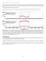
User Manual for SweepFinder2
Michael DeGiorgio, Christian D. Huber, Melissa J. Hubisz, Ines Hellmann,
Rasmus Nielsen
October 6, 2015
1
1. Introduction
SweepFinder2 is a program to perform genome-wide scans of selective sweeps using the spatial distribution of allele
frequencies and selective constraint in the genome. The current version of the software implements the test for sweeps
in the context of background selection of Huber et al. (2015) and DeGiorgio et al. (submitted).
If you identify any bugs or issues with the software, then please contact Michael DeGiorgio at mxd60@psu.edu to
report the issue.
If you use this software, then please cite it as
M DeGiorgio, CD Huber, MJ Hubisz, I Hellmann, R Nielsen. SweepFinder2: increased robustness and flexibility.
Submitted.
2. Installation
SweepFinder2 should run on any UNIX system. On the command line enter:
>tar -xzvf SF2.tar.gz
>cd SF2
>make
The first command decompresses the tar.gz file, the second command switches to the decompressed directory, and the
make command compiles SweepFinder2. The executable will be located in the SF2 decompressed directory.
3. Input file format
Note: If you have used a Windows operating system to generate the following input files, then you will likely need to run
the UNIX command dos2unix on each of the files before using them as input in SweepFinder2.
3.1. Allele frequency file
The allele frequency input file is tab-delimited and contains a header. Each row represents the allele frequency for a
position in the genome, and the rows are ordered by increasing position along the chromosome. There should be a
separate allele frequency file for each chromosome when performing a scan for selective sweeps. At each row, the first
column is the position on the chromosome, the second column is the allele count ( ), the third column is the sample size
( ), and the fourth column is an indicator as to whether the site has been polarized (i.e., whether it is known that the
allele is derived or ancestral). If the site is polarized, then the entry in the folded column should be 0, and the entry in
the second column should be the derived allele count . If the site is not polarized, then the entry in the folded column
should be 1. The allele count can take on values
. If
and the site is polarized, then the site is
monomorphic and the allele is identical to the outgroup used to polarize the site. If
and the site is polarized, then
the site is a substitution (monomorphic and different from the outgroup used to polarize the site). Otherwise, the site is
a polymorphism. Based on the study of Huber et al. (2015), we do not recommend using sites with
when the
site is polarized. That is, we recommend only using polymorphisms and substitutions to scan for sweeps. An example
input file is (say for chromosome 6):
position
460000
460010
460210
463000
…
x
9
100
30
0
…
2
n
100
100
78
94
…
folded
0
0
1
0
…
The first line of the example input file displays the header, which must be identical to this example. The next four rows
display allele frequency data for four positions on a chromosome (positions 460000, 460010, 460210, and 463000). Each
row indicates the number of derived alleles observed (and the total number of alleles observed) at the given
chromosomal position. At position 460000, 9 derived alleles were observed out of 100 total alleles (50 diploid
individuals) leading to an observed polymorphism in the sample. At position 460010, 100 derived alleles were observed
out of 100 total alleles (50 diploid individuals) leading to an observed substitution in the sample. At position 460210, 30
alleles of one type were observed out of 78 total alleles (39 diploid individuals), leading to another observed
polymorphism in the sample. Note that at this row we set folded to 1 because we were not sure whether the allele was
derived or ancestral. At position 463000, no derived alleles were observed out of 94 total alleles (47 diploid individuals),
leading to an observed monomorphic site that is identical to the outgroup in the sample. If the true sample size was 50
diploid individuals, then positions 460210 and 463000 would be genomic positions with missing data in the sample.
3.2. Recombination file
The recombination rate input file is tab-delimited and contains a header. Each row represents the recombination rate in
centiMorgans (cM) between the position in the genome and the previous position in the file, and the rows are ordered
by increasing position along the chromosome. Every position, and only those positions, in the allele frequency input file
should be included in the respective recombination input file. There should be a separate recombination rate file for
each chromosome when performing a scan for selective sweeps. At each row, the first column is the position on the
chromosome and the second column is the recombination rate in cM. For the first position in the input file the
recombination rate is 0. An example recombination input file matching the above example allele frequency input file:
position
460000
460010
460210
463000
…
rate
0.0
0.0001
0.002
0.0279
…
The first line of the example input file displays the header, which must be identical to this example for every
recombination input file. The next four rows display recombination rates (in cM) for four positions on a chromosome
(positions 460000, 460010, 460210, and 463000). At position 460000, the rate is 0, because it is the first position in the
file. The rate between positions 460000 and 460010 is 0.0001 cM, between positions 460010 and 460210 is 0.002 cM,
and between positions 460210 and 463000 is 0.0279 cM.
3.3. B-value file
The B-value input file is tab-delimited and contains a header. Each row represents the B-value at the position in the
genome, and the rows are ordered by increasing position along the chromosome. Every position, and only those
positions, in the allele frequency input file should be included in the respective B-value input file. There should be a
separate B-value file for each chromosome when performing a scan for selective sweeps. At each row, the first column
is the position on the chromosome and the second column is the B-value. An example B-value input file matching the
above example allele frequency input file:
position
460000
460010
460210
463000
…
bvalue
0.2
0.5
0.95
1.0
…
The first line of the example input file displays the header, which must be identical to this example for every B-value
input file. The next four rows display B-values for four positions on a chromosome (positions 460000, 460010, 460210,
3
and 463000). At position 460000, the B-value is 0.2, indicating a strong reduction in diversity is expected due to
background selection. The B-value at position 460010 is 0.5, indicating that background selection reduces diversity by
50% at that site. The B-value at position 460210 is 0.95 indicating that background selection had minimal impact on
diversity at this site. Finally, the B-value at position 463000 is 1.0, indicating that background selection has no impact on
diversity at this site.
3.4. User-defined grid file
The user-defined grid input file has a simple format with a single position on each row (there is no header). Each position
will specify a genomic location at which the test statistic will be computed. The positions in the user-defined grid file
should be spanned by the range of positions in the allele frequency input file. Only those positions in the user-defined
grid file will have a selective sweep computed. That is, providing a user-defined grid file overrides the uniform grid
option that is default to SweepFinder2. An example user-defined grid input file:
460000
460010
460210
463000
…
The first four rows indicate that a test for selective sweeps will be computed at positions 460000, 460010, 460210, and
463000.
4. Helper file (useful for genome-wide scans of selective sweeps)
In many circumstances, it is desirable to calculate the frequency spectrum across the whole genome and to use this
frequency spectrum as the allele frequency distribution under the null hypothesis of neutrality. It is required that the
user first combine their allele frequency files into a single allele frequency file with exactly the same format as the
example in section 3.1, and we will refer to this file as CombinedFreqFile. The reason to create this combined allele
frequency file is to generate genome-wide estimates of the empirical frequency spectrum. As an example, suppose we
have data from each of the 22 human autosomes, and each chromosome has its own allele frequency file called
FreqFile_k,
. The CombinedFreqFile would have all of the data contained in
FreqFile_k
, in one file. There would be a line in CombinedFreqFile for each of the data lines
contained in FreqFile_k,
.
4.1. Compute empirical frequency spectrum (-f)
To compute the empirical frequency spectrum, use the –f option (identical to the command from the original version of
SweepFinder). The command is:
./SweepFinder2 –f CombinedFreqFile SpectFile
where CombinedFreqFile is an allele frequency input file combined across all chromosomes in the analysis (to get a
genome-wide estimate) and SpectFile is the name of a file where the results will be printed.
5. Scanning for selective sweeps
5.1. Scan for selective sweeps
To perform a scan for selective sweeps with the original method of Nielsen et al. (2005), use the -s option. The
command to perform this scan is
4
./SweepFinder2 -s G FreqFile OutFile
where G is a user-defined number of grid points ( test sites are equally spaced across the genomic region spanned by
the positions in FreqFile) to compute the test statistic, FreqFile is the allele frequency input file, and OutFile is
the name of a file where the results will be printed. Here, FreqFile would be for a specific chromosome (or region of
the genome) rather than combined across all chromosomes.
Sometimes it is more convenient to set the spacing between grid points rather than the number of grid points. The user
may specify the approximate desired spacing between test sites using the –sg option. The command to perform this
scan is
./SweepFinder2 –sg g FreqFile OutFile
where g is a user-defined space between grid points. For example, if the user desired a test site approximately every
one kilobase, then
, representing 1000 nucleotides.
Further, it can often be useful to use a custom grid of test sites rather than a uniform grid. The user may specify this
custom grid using the –su option. The command to perform this scan is
./SweepFinder2 –su GridFile FreqFile OutFile
where GridFile is a user-defined grid input file defined in section 3.4.
5.2. Scan for selective sweeps with pre-computed empirical spectrum
To perform a scan for selective sweeps with the original method of Nielsen et al. (2005) and a pre-computed empirical
frequency spectrum, use the -l option. The command to perform this scan is
./SweepFinder2 -l G FreqFile SpectFile OutFile
where G is a user-defined number of grid points ( test sites are equally spaced across the genomic region spanned by
the positions in FreqFile) to compute the test statistic, FreqFile is the allele frequency input file, SpectFile is
an input file containing the empirical derived allele frequency spectrum calculated using the –f option in section 4.1,
and OutFile is the name of a file where the results will be printed. Here, FreqFile would be for a specific
chromosome (or region of the genome) rather than combined across all chromosomes.
Sometimes it is more convenient to set the spacing between grid points rather than the number of grid points. The user
may specify the approximate desired spacing between test sites using the –lg option. The command to perform this
scan is
./SweepFinder2 –lg g FreqFile SpectFile OutFile
where g is a user-defined space between grid points. For example, if the user desired a test site approximately every
one kilobase, then
, representing 1000 nucleotides.
Further, it can often be useful to use a custom grid of test sites rather than a uniform grid. The user may specify this
custom grid using the –lu option. The command to perform this scan is
./SweepFinder2 –lu GridFile FreqFile SpectFile OutFile
where GridFile is a user-defined grid input file defined in section 3.4.
5
5.3. Scan for selective sweeps with pre-computed empirical spectrum and recombination
map
To perform a scan for selective sweeps with a pre-computed empirical frequency spectrum and a recombination map,
use the -lr option. The command to perform this scan is
./SweepFinder2 –lr G FreqFile SpectFile RecFile OutFile
where G is a user-defined number of grid points ( test sites are equally spaced across the genomic region spanned by
the positions in FreqFile) to compute the test statistic, FreqFile is the allele frequency input file, RecFile is the
respective recombination rate file, SpectFile is an input file containing the empirical derived allele frequency
spectrum calculated using the –f option in section 4.1, and OutFile is the name of a file where the results will be
printed. Here, FreqFile and RecFile would be for a specific chromosome (or region of the genome) rather than
combined across all chromosomes.
Sometimes it is more convenient to set the spacing between grid points rather than the number of grid points. The user
may specify the approximate desired spacing between test sites using the –lrg option. The command to perform this
scan is
./SweepFinder2 –lrg g FreqFile SpectFile RecFile OutFile
where g is a user-defined space between grid points. For example, if the user desired a test site approximately every
one kilobase, then
, representing 1000 nucleotides.
Further, it can often be useful to use a custom grid of test sites rather than a uniform grid. The user may specify this
custom grid using the –lru option. The command to perform this scan is
./SweepFinder2 –lru GridFile FreqFile SpectFile RecFile OutFile
where GridFile is a user-defined grid input file defined in section 3.4.
5.4. Scan for selective sweeps with pre-computed empirical spectrum and B-value map
To perform a scan for selective sweeps with a pre-computed empirical frequency spectrum and a recombination map,
use the –lb option. The command to perform this scan is
./SweepFinder2 –lb G FreqFile SpectFile BValFile N1 N2 T OutFile
where G is a user-defined number of grid points ( test sites are equally spaced across the genomic region spanned by
the positions in FreqFile) to compute the test statistic, FreqFile is the allele frequency input file, BvalFile is
the respective B-value file, N1 is current ingroup effective population size, N2 is ancestral effective population size, T is
the divergence time in generations between the ingroup and the outgroup, SpectFile is an input file containing the
empirical derived allele frequency spectrum calculated using the –f option in section 4.1, and OutFile is the name of
a file where the results will be printed. Here, FreqFile and BValFile would be for a specific chromosome (or region
of the genome) rather than combined across all chromosomes.
Sometimes it is more convenient to set the spacing between grid points rather than the number of grid points. The user
may specify the approximate desired spacing between test sites using the –lbg option. The command to perform this
scan is
6
./SweepFinder2 –lbg g FreqFile SpectFile BValFile N1 N2 T OutFile
where g is a user-defined space between grid points. For example, if the user desired a test site approximately every
one kilobase, then
, representing 1000 nucleotides.
Further, it can often be useful to use a custom grid of test sites rather than a uniform grid. The user may specify this
custom grid using the –lbu option. The command to perform this scan is
./SweepFinder2 –lbu GridFile FreqFile SpectFile BValFile N1 N2 T OutFile
where GridFile is a user-defined grid input file defined in section 3.4.
5.5. Scan for selective sweeps with pre-computed empirical spectrum, recombination map,
and B-value map
To perform a scan for selective sweeps with a pre-computed empirical frequency spectrum and a recombination map,
use the –lrb option. The command to perform this scan is
./SweepFinder2 –lrb G FreqFile SpectFile RecFile BValFile N1 N2 T OutFile
where G is a user-defined number of grid points ( test sites are equally spaced across the genomic region spanned by
the positions in FreqFile) to compute the test statistic, FreqFile is the allele frequency input file, RecFile is the
respective recombination rate file, BvalFile is the respective B-value file, N1 is current ingroup effective population
size, N2 is ancestral effective population size, T is the divergence time in generations between the ingroup and the
outgroup, SpectFile is an input file containing the empirical derived allele frequency spectrum calculated using the
–f option in section 4.1, and OutFile is the name of a file where the results will be printed. Here, FreqFile,
RecFile, BValFile would be for a specific chromosome (or region of the genome) rather than combined across all
chromosomes.
Sometimes it is more convenient to set the spacing between grid points rather than the number of grid points. The user
may specify the approximate desired spacing between test sites using the –lrbg option. The command to perform this
scan is
./SweepFinder2 –lrbg g FreqFile SpectFile RecFile BValFile N1 N2 T OutFile
where g is a user-defined space between grid points. For example, if the user desired a test site approximately every
one kilobase, then
, representing 1000 nucleotides.
Further, it can often be useful to use a custom grid of test sites rather than a uniform grid. The user may specify this
custom grid using the –lrbu option. The command to perform this scan is
./SweepFinder2 –lrbu GridFile FreqFile SpectFile RecFile BValFile N1 N2 T OutFile
where GridFile is a user-defined grid input file defined in section 3.4.
6. Examples
The example_input directory provides example input files. For the following commands, we assume that executable
SweepFinder2 is located in the same directory as the example files.
7
There are three sets of files, a background frequency spectrum from neutral simulations, files generated from
simulations with only background selection, and files generated from simulations with both background and positive
selection.
List of files from neutral simulations:
Neutral_background.sfs.invar0
Derived SFS for counts
Neutral_background.sfs.invar1
Derived SFS for counts
Neutral_background.sfs.invar2
Derived SFS for counts
List of files from simulations with only background selection:
BGS_noSweep.SF.65.invar0
Allele frequencies for counts
BGS_noSweep.SF.65.invar1
Allele frequencies for counts
BGS_noSweep.SF.65.invar2
Allele frequencies for counts
BGS_noSweep.Rec_map.65.invar0
BGS_noSweep.Rec_map.65.invar1
BGS_noSweep.Rec_map.65.invar2
Recombination map for counts
Recombination map for counts
Recombination map for counts
BGS_noSweep.Bval_map.65.invar0
BGS_noSweep.Bval_map.65.invar1
BGS_noSweep.Bval_map.65.invar2
B-value map for counts
B-value map for counts
B-value map for counts
List of files from simulations with both background and positive selection:
BGS_Sweep.SF.84.invar0
Allele frequencies for counts
BGS_Sweep.SF.84.invar1
Allele frequencies for counts
BGS_Sweep.SF.84.invar2
Allele frequencies for counts
BGS_Sweep.Rec_map.84.invar0
BGS_Sweep.Rec_map.84.invar1
BGS_Sweep.Rec_map.84.invar2
Recombination map for counts
Recombination map for counts
Recombination map for counts
BGS_Sweep.Bval_map.84.invar0
BGS_Sweep.Bval_map.84.invar1
BGS_Sweep.Bval_map.84.invar2
B-value map for counts
B-value map for counts
B-value map for counts
Here is an example of using SweepFinder2 to identify selective sweeps under simulations with only background
selection, but while using an input recombination map but not an input B-value map. The output of this analysis will
produce output used for the black dots in Figure 1A below.
./SweepFinder2 -lr 100 BGS_noSweep.SF.65.invar1 Neutral_Background.sfs.invar1
BGS_noSweep.Rec_map.65.invar1 Out.txt
Here is an example of using SweepFinder2 to identify selective sweeps under simulations with only background
selection, but while using input recombination and B-value maps. The output of this analysis will produce output used
for the red dots in Figure 1A below.
./SweepFinder2 -lrb 100 BGS_noSweep.SF.65.invar1 Neutral_Background.sfs.invar1
BGS_noSweep.Rec_map.65.invar1 BGS_noSweep.Bval_map.65.invar1 250 250 2000 Out.txt
Here is an example of using SweepFinder2 to identify selective sweeps under simulations with both background and
positive selection, but while using an input recombination map but not an input B-value map. The output of this analysis
will produce output used for the black dots in Figure 1B below.
./SweepFinder2 -lr 100 BGS_Sweep.SF.84.invar1 Neutral_Background.sfs.invar1
8
BGS_Sweep.Rec_map.84.invar1 Out.txt
Here is an example of using SweepFinder2 to identify selective sweeps under simulations with both background and
positive selection, but while using input recombination and B-value maps. The output of this analysis will produce
output used for the red dots in Figure 1B below.
./SweepFinder2 -lrb 100 BGS_Sweep.SF.84.invar1 Neutral_Background.sfs.invar1
BGS_Sweep.Rec_map.84.invar1 BGS_Sweep.Bval_map.84.invar1 250 250 2000 Out.txt
Figure 1: Results from applying SweepFinder2 to data simulated with background selection. (A,B) Composite likelihood
ratio test statistics as a function of position along a sequence without (A) and with (B) a fixed selective sweep in the
center of the sequence. The gray region represents a reduction in recombination rate by two orders of magnitude.
Including the B-value map decreases false inferences of positive selection (A), yet still can identify positively-selected
alleles in regions with background selection (B).
7. References
CD Huber, M DeGiorgio, I Hellmann, R Nielsen (2015) Detecting recent selective sweeps while controlling for mutation
rate and background selection. Mol Ecol doi:10.111/mec.13351.
M DeGiorgio, CD Huber, MJ Hubisz, I Hellmann, R Nielsen. SweepFinder2: increased robustness and flexibility. Submitted.
R Nielsen, S Williamson, Y Kim, MJ Hubisz, AG Clark, C Bustamante (2005) Genomic scans for selective sweeps using SNP
data . Genome Res. 15:156-1575.
9