Download Time Series Modelling using TSMod 3.24

econstor
www.econstor.eu
Der Open-Access-Publikationsserver der ZBW – Leibniz-Informationszentrum Wirtschaft
The Open Access Publication Server of the ZBW – Leibniz Information Centre for Economics
Bos, Charles S.
Working Paper
Time Series Modelling using TSMod 3.24
Tinbergen Institute Discussion Paper, No. 03-091/4
Provided in Cooperation with:
Tinbergen Institute, Amsterdam and Rotterdam
Suggested Citation: Bos, Charles S. (2003) : Time Series Modelling using TSMod 3.24,
Tinbergen Institute Discussion Paper, No. 03-091/4
This Version is available at:
http://hdl.handle.net/10419/85889
Nutzungsbedingungen:
Die ZBW räumt Ihnen als Nutzerin/Nutzer das unentgeltliche,
räumlich unbeschränkte und zeitlich auf die Dauer des Schutzrechts
beschränkte einfache Recht ein, das ausgewählte Werk im Rahmen
der unter
→ http://www.econstor.eu/dspace/Nutzungsbedingungen
nachzulesenden vollständigen Nutzungsbedingungen zu
vervielfältigen, mit denen die Nutzerin/der Nutzer sich durch die
erste Nutzung einverstanden erklärt.
zbw
Leibniz-Informationszentrum Wirtschaft
Leibniz Information Centre for Economics
Terms of use:
The ZBW grants you, the user, the non-exclusive right to use
the selected work free of charge, territorially unrestricted and
within the time limit of the term of the property rights according
to the terms specified at
→ http://www.econstor.eu/dspace/Nutzungsbedingungen
By the first use of the selected work the user agrees and
declares to comply with these terms of use.
TI 2003-091/4
Tinbergen Institute Discussion Paper
Time Series Modelling using
TSMod 3.24
Charles S. Bos
Department of Econometrics and Operations Research, Vrije Universiteit Amsterdam, and Tinbergen
Institute.
Tinbergen Institute
The Tinbergen Institute is the institute for
economic research of the Erasmus Universiteit
Rotterdam, Universiteit van Amsterdam, and Vrije
Universiteit Amsterdam.
Tinbergen Institute Amsterdam
Roetersstraat 31
1018 WB Amsterdam
The Netherlands
Tel.:
Fax:
+31(0)20 551 3500
+31(0)20 551 3555
Tinbergen Institute Rotterdam
Burg. Oudlaan 50
3062 PA Rotterdam
The Netherlands
Tel.:
Fax:
+31(0)10 408 8900
+31(0)10 408 9031
Please send questions and/or remarks of nonscientific nature to driessen@tinbergen.nl.
Most TI discussion papers can be downloaded at
http://www.tinbergen.nl.
Time Series Modelling using TSMod 3.24
Charles S. Bos
Tinbergen Institute and Department of Econometrics & O.R.,
Vrije Universiteit Amsterdam
De Boelelaan 1105, NL-1081 HV Amsterdam, The Netherlands
E-mail: cbos@feweb.vu.nl
3 November 2003
Abstract
TSMod is an interactive program which allows the user to estimate a broad range of
univariate models. This review describes the possibilities of the package, from a user’s
perspective and with a secondary focus on the numerical accuracy of the program.
Keywords: Time series, software, econometrics.
1
Introduction
Performing applied econometrics is partly science, partly an art. One tends to start with
a data series, and wonder what the internal relations between observations could be. And
so start the artistic part of the analysis, trying out different types of models, judging what
might work and what is not useful. For this purpose, you rummage through the econometric toolbox which over the last decades got filled with modelling tools like the Box-Jenkins
ARIMA structure, extensions allowing for fractional integration, ideas on where regressors
might come into the system, different disturbance structures, switching models, non-linearity,
heteroskedasticity of various types, etc. etc.
For the more theoretically minded, there is often no other solution but to implement the
exact method which is needed, to have full control, while for many applications it suffices to
have available a general program which is capable of estimating a series of models easily and
in a comparable fashion, to quickly track down the model which would fit the data at hand.
TSMod, short for Time Series Modelling, is a program written by James Davidson which
can be used for such a purpose. In this review, the capabilities of TSMod, background
and relation to other programs, are described in Section 2. Section 3 describes numerical
results for a real world example and for two reference datasets, and is followed by Section
4 describing a few points that could be improved upon in future versions of the program.
Section 5 concludes.
2
Overview
2.1
General
TSMod is program program developed by James Davidson of Cardiff University. It evolved
from an earlier Ox (Doornik 1999) package for long memory modelling, intended to provide
a framework from which to teach students the basics of Econometrics and which could serve
at the same time to estimate, forecast and analyse in many ways a range of econometric
univariate time series models.
It is available free of charge for use in academic research and teaching, provided that
the usage of TSMod is acknowledged through a reference to the accompanying manual
(Davidson 2003a). The latest version of the program can be downloaded from Davidson’s
homepagehttp://www.cf.ac.uk/carbs/econ/davidsonje/. At time of writing, version 3.24
is available, though the program is clearly under ongoing development, with minor updates
and new revisions appearing regularly.
2.2
Technicalities
Time Series Modelling can be considered a program, in the sense that it comes with its own
Graphical User Interface (GUI), but could also be considered as an Ox package. TSMod
consists of a series of routines written in Ox with an OxJapi (Choirat and Seri 2002) (or
Java) shell around them, and graphical output using GnuPlot (http://www.gnuplot.info/)
through GnuDraw (Bos 2003). Since TSMod itself is written in Ox, it runs on an any platform
where Ox can be used, and where OxJapi is available as well. The program has been tested
on Windows and Linux platforms, but other operating systems should not pose any problems.
The user is responsible for getting Ox and Java working, and GnuPlot if the operating
system is of the Unix family. The GnuPlot executable for Windows is included with the
TSMod installation package.
As such, installation is easy. On Windows, it’s a matter of unzipping the installation file
into the directory for Ox packages, and possibly creating a shortcut to the batch-file starting
TSMod. On Unix, or more specifically Linux, the user has to assure that the Java executable
can be found by the operating system,1 and that GnuPlot is installed. Again, a desktop
shortcut starting the program is easily created. Without the shortcut, TSMod can be started
with the magic command oxl -s5000,5000 <path-to-TSMod>/TSMod_Run.ox, but the use
of the shortcut is advisable.
The installation comes with extensive documentation in the form of PDF manuals (Davidson 2003a, 2003b, 2003c), a version in HTML, and internally in the program itself help is
available on the menus and on the meaning of the myriad of options.
2.3
Model, features and estimation
The main model is built up around the Box-Jenkins structure for Autoregressive Integrated
Moving Average (ARIMA) models, see the General model in Table 1, or alternatively a bilinear
model can be used. Instead of an integer order of integration, also fractional integration (FI)
1
is implemented. The disturbance terms ut = ht2 et , et ∼ i.i.d.(0, 1) can have fixed variances ht
1
On a Red Hat system, a symbolic link in the /usr/local/bin directory created using ln -s
/usr/java/j2re1.4.2/bin/java does the trick.
2
or follow the asymmetric power autoregressive conditional heteroskedasticity (APARCH) or
exponential generalised ARCH (EGARCH) specifications of the table. The standard GARCH
specification is a special case of the APARCH specification, with η = 2. When using maximum
likelihood estimation, the underlying densities can be specified as either Gaussian or (possibly
skewed) Student-t. Regressors xjt , j = 1, . . . , 6 contain explanatory variables, influencing the
1/2
model at different levels. It is possible to include ht or ht in xjt , j = 1, 2, 3.
General model
Table 1: Model specifications
(1 − L)d1 Φ(L)(Yt − γ01 − γ1 t − π10 x1t ) =
γ02 + π20 x2t + Θ(L)(π30 x3t + ut ).
Bilinear alternative
Φ(L)wt = γ02 + π20 x2t + (λ(L)vt−1 )Ψ(L)wt−1 + Θ(L)vt ,
wt = (1 − L)d1 (Yt − γ10 − γ1 t − π10 x1t ),
vt = π30 x3t + ut .
APARCH
β(L)(h¡t − ω − π40 x4t ) = π50 x5t
¢
+ β(L) − (1 + α((1 − L)d2 − 1))δ(L) ((1 + µst )|ut |η + π60 x6t ).
EGARCH
η/2
β(L)(log ht − ω − π40 x4t ) = π50 x5t
¡
¢ −1
+ β(L) − (1 + α((1 − L)d2 − 1))δ(L) (ht 2 (|ut | + µut ) + π60 x6t ).
The manual (Davidson 2003a) contains full details on the possible models, but the structure is rich enough to comprise ARIMA and ARFIMA models, with APARCH/FIAPARCH/
Hyperbolic APARCH/threshold ARCH/GARCH-M resp. EGARCH-based versions. Furthermore, linear and nonlinear equations can be specified, and all kind of exogenous regressors
taken up into the analysis. The parameters in the models can be made dependent upon (unobserved) regimes, allowing for Markov Switching models (Hamilton 1989) or smooth transition
regime switching. Apart from prespecified models, with a little bit of Ox programming experience, the user can also specify a residual function to optimise whatever other (nonlinear)
function using the TSMod package, see the example on nonlinear regression in Section 3.2.
Estimation options include (Nonlinear) Least Squares, Generalised Method of Moments,
(Conditional) Maximum Likelihood and Whittle estimation in the frequency domain. The
maximum likelihood estimators condition on the first observations for applying the ARMA
filter, whereas for fractional integration the finite approximation to the infinite lag fractional
difference operator is applied. Filtering the data delivers residuals, whose likelihood is computed according densities described above. When no dynamic specification is present, the
TSMod can be triggered to use ordinary least squares for a regression model, instead of the
nonlinear least squares used otherwise. The program allows the residuals to be stored for
further analysis.
2.4
Usage
After starting TSMod, the program comes up with the main window. Initially, the user is
presented with the options to load old settings, data, change some general estimation and
output options, or work through the help menu.
The real work starts after loading a dataset. The data should be prepared to correspond
to the Ox standard for data files, which in general means that basic ASCII, Excel, Lotus or
GiveWin files can be read without problem. TSMod provides basic data editing capabilities,
3
including the possibility to add basic (log, difference, power etc.) transformations of existing
variables. Individual variables can be plotted, and summary statistics are available as well to
check that the data is read correctly.
Figure 1: A typical desktop with TSMod option dialogs and graphical output
Menus are mostly self explanatory. The user manual (Davidson 2003c) provides further
details, and its information will not be copied here. Note that many menus are ‘sticky’,
meaning that separate option dialogs can be left open on the desktop for easily changing the
settings. See Figure 1 for an example desktop with many open dialogs.
Given a data set, it is easy to specify a model by selecting the number of ARMA lags,
choosing whether the parameter d of fractional integration should be estimated, and specifying
the error structure. The model is estimated at the press of a button, and tends to be quick;
after estimation a large selection of test statistics is printed, and several diagnostic plots can
be chosen from the menu.
The usage is simple enough for students to use in class, and offers enough possibilities for
practitioners to use TSMod as a valuable tool. However, it should be noted that the package
is not commercial, which is noted from the occasional bug. See also Section 4.
2.5
Competitors
As TSMod is a program to analyse time series, it has several competitors. In the commercial
range the most well-known are EViews, TSP and PcGive. Among the ‘free’ or open source
programs, Gretl comes to mind, which has more extensive data editing capabilities, but is
mostly intended for undergraduate use with regression models, less specifically targeted at
4
time series models.
3
3.1
Numerical details
Inflation and long memory
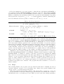
To test the functionality and numerical accuracy, the dataset analysed in Bos, Franses and
Ooms (1999) is loaded into TSMod. The series concerns the U.S. price level, 2 see the article
for details. The inflation series derived from the price levels is modelled using a long memory
model, accounting for level shifts around the oil crises; in the article break points at 1973:07,
1976:07, 1979:01 and 1982:07 are used.
Originally, the ARFIMA-X(12, d, 0) model, with breaks and restrictions on AR parameters
φ2 = . . . = φ11 = 0, is estimated using Gauss with an approximative Whittle likelihood
function in the frequency domain. Alternatively, it is possible to use the ARFIMA package
(Doornik and Ooms 2001, Doornik and Ooms 2003) for Ox which implements the exact
maximum likelihood (EML) in the time domain, using methods of Sowell (1992). And the
third option is to use TSMod, with the conditional maximum likelihood (CML) procedure.
Results of these three estimation methods are provided in Table 2.
d
φ1
φ12
γ73:07
γ76:07
γ79:01
γ82:07
Table 2: Estimation results on inflation data
Gauss (Whittle)
Ox (EML)
TSM (CML)
θ̂
σθ
θ̂
σθ
θ̂
σθ
σθ robust
0.3808 (0.057)
0.3805 (0.050)
0.3895 (0.056)
[0.066]
−0.2020 (0.068)
−0.2104 (0.064)
−0.2100 (0.067)
[0.089]
0.0593 (0.047)
0.0597 (0.047)
0.0588 (0.045)
[0.046]
0.4212 (0.102)
0.2990 (0.102)
0.2758 (0.101)
[0.255]
−0.0631 (0.112)
−0.0361 (0.112)
−0.0433 (0.112)
[0.131]
0.2480 (0.111)
0.2770 (0.111)
0.2728 (0.111)
[0.104]
−0.5342 (0.100)
−0.5322 (0.102)
−0.5363 (0.103)
[0.103]
Results of estimating an ARFIMA-X(12,d,0) model on U.S. inflation data, using three different
estimation methods. Reported are the parameter estimates and standard deviations. TSMod can
report either ‘standard’ or ‘robust’ standard deviations.
The results indicate that, even for a model which is notoriously hard to estimate, the
three slightly different models result in very similar outcomes. For most practical purposes,
these estimates can be considered equal. Note that some difference was expected, as the
likelihood functions are not equal: Gauss estimates in the frequency domain, whereas Ox (or
the ARFIMA package used through Ox) and TSMod differ in the manner in which the first
observations are used for conditioning.
Note that TSMod defaults to reporting standard errors based on the combination of the
Hessian and the outer product of the gradient, which is more robust in the case of misspecification of the likelihood function. The last column of Table 2 reports these robust standard
deviations. Alternatively, TSMod can provide heteroskedasticity consistent estimates of the
covariance matrix and standard deviation, according to the formula of Newey and West (1987).
2
Source: Bureau of Labor Statistics, series SA0, 1957:1–1995:12. Inflation series were constructed using
100∆ ln st , and the main effect of seasonality was taken out of the series by regressing on a set of seasonal
dummies.
5
Equation for dLPs
0.3
Conditional Variances
0.25
0.2
0.15
0.1
0.05
0
1964
1970
1976
1982
1988
1994
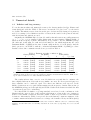
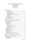
Figure 2: Conditional variance estimate for an ARFIMA(12,d,0)-GARCH model on inflation
With these results, the user can continue specifying e.g. GARCH-type heteroskedasticity.
Easily a graph like Figure 2 is extracted, displaying the jump in volatility in the beginning
of the first oil crisis. TSMod works very well in quickly trying out different specifications,
combinations of breaks with GARCH or long memory, and can be a very useful tool.
3.2
Two reference data sets
The Statistical Engineering and the Mathematical and Computational Sciences divisions of
the National Institute of Standards and Technology provides a collection of statistical reference datasets at http://www.itl.nist.gov/div898/strd/. For these data sets, the model
and the optimum values are reported up to a high degree of precision. As a test of the TSMod
package, two of the datasets are tried here.
Linear regression with unbalanced regressors
The first one is a linear regression model, where the data is chosen such that estimation is
cumbersome. The model itself is simply
y=
10
X
βi xi + ²,
i=0
see http://www.itl.nist.gov/div898/strd/lls/data/Filip.shtml for details.
The dataset is most easily prepared in another program like Excel or Ox, as the editing
capabilities of TSMod only allow for the usual transformations as squaring or cubing the data,
not for computing xi , i > 3.3
With the data loaded in TSMod, estimating the model is not a problem. After specifying
the regression model, estimation is immediate. The results from TSMod (using the nonrobust formula for calculating standard deviations) are exactly equal to the results as Ox
would report them. Also the fact that the matrix of regressors is unbalanced and that scaling
is advised is mentioned in the TSMod output. The parameter values and standard deviations
correspond with the reference results, for all digits reported by TSMod; only in the residual
standard deviation a small difference is found.
3
When the author heard of this limitation, it was addressed quickly in the first upgrade to TSMod which
was released after completing the review.
6
Note that equal results are only found when using the ordinary least squares estimation
method; if the model is estimated using the iterative optimisation routine and the nonlinear
least squares criterion function, the correct solution is not attained as the criterion function
is too flat.
Nonlinear regression
In the previous reference data set, a standard linear model was used. A second reference
data set, at http://www.itl.nist.gov/div898/strd/nls/data/eckerle4.shtml, concerns
a study involving circular interference transmittance as a response variable, depending on the
wavelength. The data set provided contains 35 observations. The model is
µ
¶
β1
(x − β3 )2
y=
exp −
+ ²,
(1)
β2
2β22
which can be estimated in TSMod using a user-specified function. For this purpose, an
adapted version of the file TSMod Run.ox was created with the function definition as in the
listing in Figure 3. Starting TSMod from this file, with oxl -s5000,5000 TSMod Ecker.ox,
was enough to implement the above model in TSMod.
Figure 3: Specifying a user-defined function in TSMod Ecker.ox
/*------------TIME SERIES MODELLING v3.24 RUN SPECIFICATION ------------*/
///////////////////////////////////////////////////////////////////////////
#define USER_FUNCTION
#import <packages/tsmod32/tsmgui32>
///////////////////////////////////////////////////////////////////////////
UserFunction(const mcX, const cStart, const cEnd, const vP, const sName)
{
decl vE, iX, iY;
iX= VarNum("X");
iY= VarNum("Y");
// Compute residuals
vE= mcX[][iY] - (vP[0]/vP[1]) * exp(-0.5*sqr((mcX[][iX]-vP[2])/vP[1]));
return vE[cStart:cEnd];
}
With the data set, two alternative starting vectors of βa = (1, 10, 500) or βb = (1.5, 5, 450)
are provided. From the first set of points (or from TSMod’s defaults, β = 0), no convergence
is found. The second set, closer to the optimum, leads to the results in Table 3. Up to all
digits specified by TSMod, resulting parameter values are equal to the reference results, as
is the case for the sum of squared residuals. The (non-robust) standard errors differ slightly
from the reference results.
It should be noticed that this is quite an accomplishment, as the model combined with
this data set is graded to have a higher level of difficulty. Also the ease with which the residual
function of the model can be added to TSMod is remarkable.
7
Table 3: Estimation results on Ecker nonlinear regression model
TSMod
Reference
β1
1.5544 (0.0149915)
1.55444 (0.0154080)
β2
4.0888 (0.0459662)
4.08883 (0.0468030)
β3
451.54
(0.0453601)
451.541
(0.0468005)
SSR
0.00146359
0.001463589
Results from TSMod for the Ecker data set, with reference results. The reference parameter estimates are reported with one extra digit compared to the
TSMod results. TSMod standard deviations are computed using the nonrobust formula.
4
Drawbacks and minor problems
Even though TSMod is a nice program as-is, it is not without some minor problems. It
is not a commercial product with the backing of an entire company and a long history in
bug-hunting, and therefore some issues can be found with the program. Less problematic are
bugs like an incorrect (i.e., illogical) model specification not being handled gracefully, or if
the program stops with an error message if the sample size was moved around so much that
TSMod got confused about where to start. In such cases, a restart of the program helps a
lot, which is not much of a hassle as the model specification and estimated parameter values
are saved between sessions.
In an earlier version of TSMod, there was a problem that only non-linear least squares
was available as an estimation method. If the model was purely linear, the basic regression
model which is found so often in applied work, estimation was not fully efficient as the full
gradient method was applied instead of solving the regression equation directly by ordinary
least squares. This problem may serve as a good example of the speed with which TSMod
is improving: While writing the review, a new version of the program appeared which filled
this gap. Likewise, a more serious bug in an earlier version of the program which surfaced
while working on this report, was taken out by the author of TSMod in the course of hours,
not days. New versions of the program come out regularly, either to improve on a bug, or to
elaborate further on the features of the program.
When TSMod solves a model by optimising a criterion function (be it the sum of squared
residuals or a likelihood estimate), a general purpose gradient method is used. This optimising
routine behind it all is the MaxBFGS routine of Ox, which is a high quality, gradient-type,
optimising routine. However, with the inflation data set in Section 3.1 it was quite possible
to specify a model which was of a richer structure than the data could support, e.g. by
specifying a varying variance structure when in effect the variance is constant. In such cases,
the likelihood function may well be very flat, or multimodal, and it was possible to get to
situations where TSMod had to be helped with correct starting values for the optimisation.
5
Conclusions
In this review part of the possibilities of TSMod was investigated. The wealth of models
incorporated in the package is impressive, the user interface sufficiently friendly and fullproof that even less experienced users, or students, should have little problem in estimating
their first models. It works well as a tool for comparing different model components in an
8
explanatory analysis of a data set, and even non-standard models could easily be implemented
using a user-specified function. In Section 3 it was found that the numerical accuracy of
TSMod is good, as it is able to replicate quickly and to a high precision results found in the
literature or in reference data sets.
This overview of the program is limited in the sense that only the interactive mode of
TSMod was discussed, with a small side tour to include a user specified residual function in
section 3.2. A separate document (Davidson 2003b) describes the programming interface of
TSMod, as all the routines implemented in TSMod can also be used from a user’s own Ox
application. The programming interface would however be a topic on its own, and is left for
the reader to explore.
TSMod is a useful program, it is nice to see how it keeps evolving over time, and I definitely
plan to keep a version around in order to quickly estimate a model on a data set. The fact
that it is freely available for academic use makes it a good candidate for the more advanced
Econometrics classes as well, as students tend to appreciate to be allowed to use a program
at home.
References
Bos, C. S. (2003), GnuDraw, http://www.tinbergen.nl/~cbos/gnudraw.html.
Bos, C. S., Franses, P. H. and Ooms, M. (1999), ‘Long memory and level shifts: Re-analyzing
inflation rates’, Empirical Economics 24, 427–449.
Choirat,
C.
and
Seri,
R.
(2002),
OxJapi:
an
Ox
version
of
Merten
Joost’s
Java
Application
Programming
Interface,
http://site.voila.fr/choirat/software/oxjapi/oxjapi.html.
Davidson,
J.
(2003a),
Time
Series
http://www.cf.ac.uk/carbs/econ/davidsonje/.
Modelling
Davidson, J. (2003b), Time Series Modelling Version 3.24:
http://www.cf.ac.uk/carbs/econ/davidsonje/.
Davidson, J. (2003c), Time Series Modelling Version
http://www.cf.ac.uk/carbs/econ/davidsonje/.
Version
3.24,
Programming Reference,
3.24:
User’s
Manual,
Doornik, J. A. (1999), Object-Oriented Matrix Programming using Ox, 3rd edn, Timberlake
Consultants Ltd, London. See http://www.nuff.ox.ac.uk/Users/Doornik.
Doornik, J. A. and Ooms, M. (2001), A Package for Estimating, Forecasting and Simulating
Arfima Models: Arfima Package 1.01 for Ox. Package manual.
Doornik, J. A. and Ooms, M. (2003), ‘Computational aspects of maximum likelihood estimation of autoregressive fractionally integrated moving average models’, Computational
Statistics & Data Analysis 42(3), 333–348.
9
Hamilton, J. D. (1989), ‘A new approach to the economic analysis of nonstationary time series
and the business cycle’, Econometrica 57, 357–384.
Newey, W. K. and West, K. D. (1987), ‘A simple, positive semi-definite, heteroskedasticity
and autocorrelation consistent covariance matrix’, Econometrica 55, 703–708.
Sowell, F. (1992), ‘Maximum likelihood estimation of stationary univariate fractionally integrated time series models’, Journal of Econometrics 53, 165–188.
10