Download Addendum No. 4 to

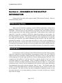
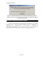
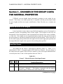
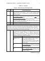
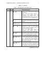
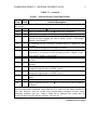
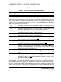
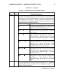
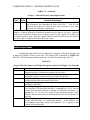
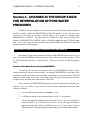
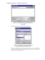
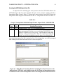
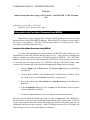
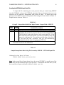
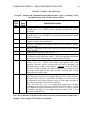
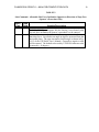
Addendum No. 4 to
UTEXAS4
A COMPUTER PROGRAM FOR SLOPE
STABILITY CALCULATIONS
By
Stephen G. Wright
May 2007
Shinoak Software
Austin, Texas
Copyright © 2007 by Stephen G. Wright - All Rights Reserved
INTRODUCTION
Section 1 - Introduction
This document supplements the original user’s manual for the UTEXAS4 and
TexGraf4 software and describes several new features. These include changes in the output
(dialog boxes) displayed by the software. They also include additions to the Group C data
for materials to accommodate laterally varying unit weights, additions to the Group E data
for interpolation of pore water pressures, and two new features in the Group K data for the
analysis and computations. These changes are described in the following sections.
Page 2 of 21
CHANGES IN OUTPUT
Section 2 – CHANGES IN THE OUTPUT
INFORMATION
Changes have been made in the output for both UTEXAS4 and TexGraf4. These are
described separately below.
UTEXAS Message Display
When you run a data file by opening it in the UTEXAS4 application, a dialog box is
displayed showing most of the various notice, warning and error messages issued by
UTEXAS4. These messages provide information on possible errors and problems related to
either the input data or the slope stability computations. Further details can be found in the
output file (*.out) that is created by UTEXAS4, where the messages are also written. For
messages pertaining to errors in input data the output file can be examined to determine what
was wrong with the input data. For messages associated with computations for a particular
slip surface the output file will contain information on the location of the slip surface that
generated the message, e.g. the center point and radius of a circle or the coordinates of a
noncircular slip surface. In most cases when error messages are issued the output file should
be examined for more details. In some cases errors in input can be readily identified from the
messages in the dialog box alone and corrected without referring to the output file for details.
TexGraf4 Notice
If an automatic search is performed with UTEXAS4 and some of the factors of safety
cannot be computed for centers immediately surrounding the critical circle, the UTEXAS4
output file has always contained a warning message to that effect. However, this information
was not apparent in TexGraf4 when results were viewed with that program (TexGraf4). Now
a feature has been added to TexGraf4 such that a similar message to the one in the
UTEXAS4 output file is now displayed. When a Graphics Exchange file is now read by
TexGraf4, TexGraf4 will display a dialog box like the one shown in Figure 3.1 to again warn
you that the factor of safety was not computed for all of the trial center points immediately
surrounding the center point with the minimum factor of safety. The detailed output file
created by UTEXAS4 should then be examined to determine why the factor of safety could
not be computed. The factor of safety may not be computed for legitimate reasons, e.g. the
slip surface intersects a very strong material, or because of an error, in which case a remedy
may need to be sought.
Page 3 of 21
CHANGES IN OUTPUT
Figure 3.1 - Dialog Box Displayed by TexGraf4 When UTEXAS4 Was Not Able to
Compute the Factor of Safety for All of the Trial Center Points Immediately Adjacent
to the Most Critical Circle
Filenames on Output Pages printed by TexGraf4
Ordinarily TexGraf4 prints on the output page the full path name of the Graphics
Exchange input file. This can be changed manually by editing a parameter in the
configuration file, TEXGRAF4.CFG.
The parameter is designated as
"FILe_PATh_NAMes_LONG" in the configuration file. Future versions of TexGraf4 will
allow this parameter to be changed and saved as part of the application preferences.
Page 4 of 21
CHANGES IN GROUP C – MATERIAL PROPERTY DATA
5
Section 3 – CHANGES IN THE GROUP C DATA
FOR MATERIAL PROPERTIES
UTEXAS4 can now handle lateral (horizontal) variations in unit weight for any
material. This feature is an added option that is compatible with the previous input format
for unit weights and does not require modification of data files that use a constant unit
weight.
Lateral Variation in Unit Weights
Lateral variations in unit weight are specified by designating a series of horizontal (x)
coordinates and the corresponding values of unit weight. Unit weights for each slice are
determined by linear interpolation in the horizontal direction based on the center coordinate,
x, of the slice. Unit weights are not extrapolated linearly outside the range specified; instead
the unit weights are considered constant beyond the first and last points. Slices to the left of
the first unit weight point specified and to the right of the last unit weight point specified will
be assigned the unit weights at the respective first and last points specified.
Input Data Format
The formats for the Group C input data are shown in Table 3.1. Table 3.1 is a
replacement for Table 7.1 from the original UTEXAS4 User’s Manual. The only change in
the format from the original UTEXAS4 user’s manual is in the unit weight information now
covered by data Lines 3 and 4 of the input data shown in Table 3.1.
TABLE 3.1
Group C - Material Property Data Input Format
Input
Line
1
Data
Field
1
2
1
Variable/Description
Command Word: "MAT" (or "MATERIAL PROPERTIES")
Number (nmaterial) used to identify the material for which data will follow
on Line(s) 3 through 7. This number corresponds with the material
numbers input for Profile Lines in the Group B data.
(continued on next page)
CHANGES IN GROUP C – MATERIAL PROPERTY DATA
6
TABLE 3.1 - continued
Group C - Material Property Data Input Format
Input
Line
2
Data
Field
2
Variable/Description
Any alphanumeric character(s) or character string(s) to be printed as a
label with data for this material. Can be as many characters and/or
blanks as will fit on a 128-character line of input (including Field 1).
Can also be blank.
3
1
Unit weight information for the current material as follows:
If unit weight is constant: Specify a numerical value, e.g. 127.5, that is
the unit weight for the material.
If the unit weight varies laterally: Specify a character or character string
starting with the character V, e.g. V or Varying unit weight
If the unit weight varies laterally follow this line of input data with
Line(s) 4; otherwise proceed to Line 5.
4
1
Horizontal (x) coordinate for unit weight point.
4
2
Unit weight (γ) at horizontal coordinate.
Repeat Line 4 for additional points to define the lateral variation in unit weight. Values
must be input in a sequence of increasing values of horizontal coordinate, x. More than one
pair of values (x and γ) can be entered on a single line of input data if desired; however,
pairs of values (even multiples of two) must always be entered on each line. Input a blank
line at the end of the data for the lateral variation in unit weights.
5
1, 2 A character or character string beginning with the appropriate character,
to designate how shear strengths are to be characterized for the current
material. The acceptable character or character string and its
interpretation are shown below. The key character(s) which must be
input are capitalized and underlined. (Note: Only the first non-blank
character of each string is recognized and used.)
Character String
Interpretation
Conventional /or/
Shear strengths are expressed by conventional
Isotropic (C or I)
Mohr-Coulomb parameters, c and φ. Follow
this line of data with line 5A below.
NOTE: Only one character or character string
should be entered to avoid confusion with ”C P”
sequence below.
Linear (L)
Shear strengths increase linearly with depth
below the Profile Line, starting at a prescribed
value along the Profile Line. Follow this line of
data with Line 5B below.
Reference (R)
Shear strengths increase linearly with depth
below a horizontal datum specified by its
reference elevation. Follow this line of data
with Line 5C below.
(continued on next page)
CHANGES IN GROUP C – MATERIAL PROPERTY DATA
7
TABLE 3.1 - continued
Group C - Material Property Data Input Format
Input
Line
5
Data
Field
1,2
Cover P ratio (C P)
Anisotropic shear (A)
Nonlinear MohrCoulomb envelope
(N)
Interpolate Strengths
(I S)
Variable/Description
The shear strength is characterized in terms of a
constant c/p ratio. Follow this line of data with
Line 5D below.
NOTE: The second leading character (P)
distinguishes
this
option
from
the
"conventional" shear strength option.
The
second character must be a "P", e. g. "C over P"
will result in the incorrect interpretation as "C
o".
Shear strengths vary with the orientation of the
failure plane. Follow this line of data with Lines
5E below.
The shear strength envelope is nonlinear.
Follow this line of data with Lines 5F below.
The shear strengths are to be determined by
interpolation of values of shear strength
specified at prescribed locations. Follow this
line of data with Lines 5G below.
NOTE: The second leading character (S)
distinguishes
this
option
from
the
"isotropic/conventional" shear strength option.
Very Strong material The soil is assumed to be infinitely strong. Any
(V S)
shear surface passing through the material is
rejected for computing the factor of safety. Line
Nos. 5, 6 and 7 are not required - omit them.
2-stage Linear
The shear strength is a "two-stage" strength and
strength envelopes
the shear strength envelopes are straight lines
(2 L)
(linear). Follow this line of data with Lines 5H
below. (Applicable only when strengths are
being entered for the second stage - otherwise an
error condition will result.)
2-stage Nonlinear
The shear strength is a "two-stage" strength and
strength envelopes
the envelope(s) are not linear. Follow this line
(2 N)
of data with Lines 5I below. (Applicable only
when strengths are being entered for the second
stage - otherwise an error condition will result.)
(continued on next page)
CHANGES IN GROUP C – MATERIAL PROPERTY DATA
8
TABLE 3.1 - continued
Group C - Material Property Data Input Format
Input
Data
Line
Field
Depending on the
etc.) is used.
6A
1
6A
2
6B
1
6B
2
Variable/Description
data entered on Input Line 4, one of the following formats (5A, 5B, 5C,
Cohesion value, c (or c ), for the soil.
Angle of internal friction, φ (or φ ), for the soil - in degrees.
Value of shear strength at the level(s) of the Profile Line.
Rate of increase in shear strength below the Profile Line, expressed as an
2
increase in shear strength per unit of depth. (Units = force/length
3
/length = force/length )
6C
1
Y coordinate for the "reference" elevation used as a datum for shear
strengths.
6C
2
Value of shear strength at the reference elevation.
6C
3
Rate of increase in shear strength below the reference elevation,
expressed as an increase in shear strength per unit of depth. (Units =
force/length2 /length = force/length3 )
6D
1
“c/p” ratio: Ratio of shear strength to effective vertical consolidation
pressure.
6D
2
“Intercept strength, co ”: Shear strength for zero effective consolidation
pressure.
6D
3
Minimum value of shear strength (This value is used to limit strengths
computed using the values in Fields 1 and 2).
6D
4
Maximum value of shear strength (This value is used to limit strengths
computed using the values in Fields 1 and 2).
6E
1
Orientation of the failure plane measured in degrees from the horizontal
plane.
6E
2
Cohesion value for current failure plane orientation.
6E
3
Angle of internal friction, φ (or φ ) for current failure plane orientation in degrees.
Repeat Line 6E for additional anisotropic shear strength values in a sequence of increasing
angles of failure plane orientation. More than one set (3 values) of data can be entered on a
given line; however, each line of data must contain integer multiples of three values,
comprising complete data sets. Input a blank line to terminate the current data for
anisotropic shear strengths and then continue with Line No. 7.
(continued on next page)
CHANGES IN GROUP C – MATERIAL PROPERTY DATA
9
TABLE 3.1 - continued
Group C - Material Property Data Input Format
Input
Data
Line
Field
Variable/Description
6F
1
Normal stress, σ (or σ ), for point on the nonlinear failure envelope
6F
2
Shear stress, τ, for point on the nonlinear envelope.
Repeat Line 6F for additional values to define a nonlinear failure envelope. Values must be
input in a sequence of increasing values of normal stress. More than one pair of values (σ
and τ) can be entered on a single line of input data if desired; however, pairs of values (even
multiples of two) must always be entered on each line. Input a blank line at the end of the
data for the nonlinear failure envelope.
6G
1
Minimum value allowed for interpolated strength. If interpolated values
are less than this value, they will be set equal to this value.
6G
2
Maximum value allowed for interpolated strength. If interpolated values
are greater than this value, they will be set equal to this value.
6H
1
Intercept, d (Kc = 1) for the envelope of τ ff vs. σfc from isotropically
consolidated-undrained triaxial compression tests.
6H
2
Slope, Ψ (Kc = 1) for the envelope of τff vs. σfc from isotropically
consolidated-undrained triaxial compression tests.
6H
3
Effective stress cohesion value, c = d (Kc = Kfailure), envelope from
consolidated-drained (CD) shear tests or consolidated-undrained shear
tests with pore pressure measurement ( CU ).
6H
4
Effective stress angle of internal friction, φ = Ψ (Kc = Kfailure), of
envelope from consolidated-drained (CD) shear tests or consolidatedundrained shear tests with pore pressure measurement ( CU ).
6I
1
Effective normal stress on the failure plane at consolidation ( σfc ) for
nonlinear two-stage envelope. The shear stresses in the next two fields
should correspond to this normal stress.
6I
2
Shear stress on the failure plane at failure ( τ ff ) for the envelope derived
from isotropically consolidated-undrained (CU) triaxial compression
tests.
6I
3
Shear stress on the failure plane at failure ( τ ff ) for the conventional
effective stress failure envelope; derived either from consolidated
drained (CD) tests or consolidated-undrained shear tests with pore water
pressure measurements( CU ).
Repeat Line 6I for additional values to define the complete nonlinear envelopes for the twostage strengths. Values must be entered in a sequence of increasing values of normal stress.
More than one set of values (points) may be entered on a single line of input data if desired;
however, each line must contain integer multiples of three values, comprising complete data
points. Input a blank line at the end of the nonlinear failure envelope data and proceed with
Line No. 6 for the current material.
(continued on next page)
CHANGES IN GROUP C – MATERIAL PROPERTY DATA
10
TABLE 3.1 - continued
Group C - Material Property Data Input Format
Input
Line
7
Data
Field
Variable/Description
1 and 2 Two characters separated by blanks, or two character strings separated
by blanks, to designate how pore water pressures are to be defined for
this material. The acceptable characters or character strings and their
interpretation are shown below. The key characters which must be input
are capitalized and underlined. (Note: Only the first character of any
character string is recognized and used.)
Character String
Interpretation
No pore pressure (N) Pore pressures are zero. (Only one character, N,
is actually required in this case.) No Line 8 is
required; see notes following Line No. 8.
Constant Pressure
Pore pressures are constant. Follow this line of
(C P)
data with Line No. 8 giving the value of the pore
water pressure.
Constant Ru (C R)
Pore water pressures are defined by a constant
value of the pore water pressure coefficient, ru.
Follow this line of data with Line No. 8 giving
the value of the pore water pressure coefficient,
ru .
Piezometric Line
A piezometric line is used to define pore water
(P L)
pressures in this material. Follow this line of data
with Line No. 8 giving the number of the
piezometric line which is to be used. Note:
Group D data must eventually be input.
Interpolate Pore
Pore water pressures are determined by
Pressures (I P)
interpolation of values of pore water pressure.
Note: Group E data must eventually be input, but
no Line No. 8 is required below. See notes
following Line No. 8.
Interpolate Ru values Pore water pressures are determined by
(I R)
interpolation of values of the pore water pressure
Note: Group E data must
coefficient, ru .
eventually be input, but no Line No. 8 is required
below.
3
Optional designation to allow negative pore water pressures. If negative
pore water pressures are allowed, enter the character “N” or a character
string beginning with the character “N” to designate that negative pore
water pressures are allowed.
(continued on next page)
CHANGES IN GROUP C – MATERIAL PROPERTY DATA
11
TABLE 3.1 - continued
Group C - Material Property Data Input Format
Input
Line
8
Data
Field
1
Variable/Description
Value of either (a) the pore water pressure, or (b) ru or (c) the number of
the piezometric line depending on data on Line No. 7. Line 8 is not
required where there are either no pore water pressures or pore water
pressures are defined by interpolation.
Repeat Lines 2 through 8, as sets, for data for additional material properties (material
numbers). Material properties for different materials may be input in any order. (Material
numbers may actually be missing from a sequence; however, there appears to be little need
for omitting numbers from a sequence.) Input a blank line after the data for the last material
have been input to designate the end of all Group C data.
Added Output Table
An additional output table has been added and is output by UTEXAS4 when the unit
weight varies laterally for one or more slice. The Output Table is identified as TABLE NO.
61 in the UTEXAS4 output and the contents are described in the following Table 3.2,
TABLE 3.2
Output Table 61 Content: Unit Weight Information when Unit Weights Vary Laterally
Column
1
2
3
4
5
6
Description
Slice Number: The number of the slice – slices are numbered from left-toright and one line of information is printed for each slice.
X-Center: The x coordinate of the center of the designated slice. This
coordinate is used to interpolate the unit weights for the slice
Matl. No.: The material number(s) for the materials in a slice. Unit
weights are listed for each material in the slice.
Height: Height of the given material at the center of the slice, i.e. at the
indicated x coordinate.
Unit Weight Stage 1: The unit weight of the designated material for the
slice indicated. If followed by the letter C in parentheses, i.e. (C), the unit
weight of the particular material is constant. If followed by the letter V in
parentheses, i.e. (V), the unit weight of the particular material varies
laterally and the value shown is the interpolated value at the mid-plane of
the slice.
Unit Weight Stage 2: Same information as Column 5, except for the
second and third stage of a multi-stage analysis. If the analysis is a
conventional, single-stage analysis the characters “N.A.” appears in this
column of the output table
CHANGES IN GROUP E – INTERPOLATION DATA
12
Section 4 – CHANGES IN THE GROUP E DATA
FOR INTERPOLATION OF PORE WATER
PRESSURES
UTEXAS4 can now import pore water pressures directly from finite element analyses
and files created by either the GMS/SEEP2D or SEEP/W software. A file with pore water
pressures at each node in the finite element mesh is first created by running either
GMS/SEEP2D or SEEP/W. The input data for UTEXAS4 is then setup so that the file
created by GMS/SEEP2D or SEEP/W will be read while reading the other UTEXAS4 input
data. Use of pore water pressures created using GMS/SEEP2D and SEEP/W is described
separately below for each program.
Interpolation with Pore Water Pressures from GMS/SEEP2D
Interpolation of pore water pressures using the GMS/SEEP2D software involves two
steps: First the GMS/SEEP2D software is run to create a file of pore water pressures. Then
the UTEXAS4 input data file is created and run. These two steps are described separately
below.
Creation of Pore Water Pressures Using GMS/SEEP2D
To create the file of pore water pressures first run GMS/SEEP2D to obtain a finite
element solution for the pore water pressures. In running GMS/SEEP2D be sure that (1) the
coordinate system is the same as the coordinate system that is to be used for the UTEXAS4
input data (same origin, same scale, same units), and (2) the pore water pressures and unit
weight of water are in the same units used for UTEXAS4.
Once you have run GMS/SEEP2D and obtained a suitable solution for the heads, pore
pressures, etc., you need to export the pore water pressure information from the GMS
software as follows:
1.
Go to the File menu and choose the Export… item.
2.
A dialog box similar to the one shown below in Fig. 4.1 is displayed:
Choose the appropriate directory into which the file is to be saved and enter a
name for the file, e. g. UTEXAS4 Pore Pressures. For the file type (see Save as
type in the dialog box) choose UTEXAS pore pressures (*.upp). Once you have
chosen a directory and entered the file name and type, click on the Save button.
CHANGES IN GROUP E – INTERPOLATION DATA
13
Figure 4.1 - Dialog Box for Exporting Information
from GMS
3.
Next, a dialog box like the following will be displayed:
Figure 4.2 - Dialog Box for Selecting Solution and
Type of Data to be Exported from GMS
Choose the solution that you want to export and select pore pressure as the data
set. When you have selected the solution and data set, click on the OK button to
export the pore water pressure data.
CHANGES IN GROUP E – INTERPOLATION DATA
14
Creating the UTEXAS4 Input Data File
To import the file containing pore water pressures into the UTEXAS4 software the
UTEXAS4 input data file must designate that pore water pressures will be entered as
Interpolation Data (Group E Data). To import pore water pressures from SEEP2D enter the
Interpolation Data using the format shown in Table 4.1. Sample data are shown in Table 4.2.
TABLE 4.1
Group E - Interpolation Point Data Input Format - Import Mode - GMS/SEEP2D
Input
Line
1
2
Data
Field
1
1
Variable/Description
Command Word: "INT" (or "INTerpolation Points")
The character string “SEEP2D” followed by the name of the file of
pore water pressure data that was created using GMS/SEEP2D, e. g.
SEEP2D UTEXAS Pore Pressures.upp. The file must be in the same
directory as the current input file. If the file cannot be located and
opened, you will be prompted to enter the name of a valid input file.
Note, that if the name of the file is omitted on Line 2 of the input data, you will be prompted
with a dialog box like the one shown below to select the input file:
Figure 4.3 - Dialog Box for Selecting the File Containing Pore Water Pressures to be
Imported into UTEXAS4 - only displayed when the File Name for importing pressures
is Omitted from the UTEXAS4 Input Data File or the designated file cannot be located.
CHANGES IN GROUP E – INTERPOLATION DATA
15
TABLE 4.2
Sample Interpolation Data Using a File Created by GMS/SEEP2D - UTEXAS4 Input
File
INTerpolation data follows SEEP2D Pore pressures.upp
Interpolation with Pore Water Pressures from SEEP/W
Interpolation of pore water pressures using the SEEP/W software involves two steps
similar to those for the GMS/SEEP2D software: First the SEEP/W software is run to create a
file of pore water pressures. Then the UTEXAS4 input data file is created and run. These
two steps are described separately below.
Creation of Pore Water Pressures Using SEEP/W
To create a file containing pore water pressures run SEEP/W in the normal way. It is
assumed that you have the software and know how to use it. Once you have completed the
analysis, examine the results using the CONTOUR module of SEEP/W. The CONTOUR
module is used to create the file that is imported by UTEXAS4. The following steps are used
to create the data file using version 4.23 of SEEP/W and the CONTOUR module; other
versions of the software may differ from this and appropriate changes may be required:
1. Choose Graph from the Draw menu. The Draw Graph dialog box should then
be displayed.
2. Click on the box labeled “View All Data Only” so that the box is checked. Then,
for “Graph Type” choose Pressure from the list of graph types.
3, Next click on the button labeled Data; the Graph Data dialog box should then be
displayed.
4. In the Graph Data dialog box click on Space for the delimiter used to separate
columns of numbers in the file.
5. Click on the SaveAs button to now save the pore water pressure data file.
The file created by SEEP/W should begin with two lines of alphanumeric text, followed by
the data for pore water pressures at each node point from the finite element mesh. Each line
of pore water pressure data will contain four values: the number of the node point, the x-y
coordinates and the pore water pressure. When UTEXAS4 reads this file it will ignore the
first two lines of text as well as the numbers of each node.
CHANGES IN GROUP E – INTERPOLATION DATA
16
Creating the UTEXAS4 Input Data File
To import the file containing pore water pressures that you created using SEEP/W
into the UTEXAS4 software the UTEXAS4 input data file must designate that pore water
pressures will be entered as Interpolation Data (Group E Data). To import pore water
pressures from SEEP/W enter the Interpolation Data using the format shown in Table 4.3.
Sample data are shown in Table 4.4.
TABLE 4.3
Group E - Interpolation Point Data Input Format - Import Mode - SEEP/W
Input
Line
1
2
Data
Field
1
1
Variable/Description
Command Word: "INT" (or "INTerpolation Points")
The character string “SEEPW” followed by the name of the file
containing the pore water pressures that was created using SEEP/W.
The file must be in the same directory as the current input file. If the
file cannot be located and opened, you will be prompted to enter the
name of a valid input file. You can also omit the name of the file, i.
e. just enter the word “GeoSlope”, and you will automatically
prompted for the file name when you run UTEXAS4.
Note: The data for interpolation points in the SEEP/W file must be in the format
described elsewhere in this Addendum.
Table 4.4
Sample Interpolation Data Using File Created by SEEP/W - UTEXAS4 Input File
INTerpolation data follows SEEPW SEEPW Pore pressures.dat
Note: In the second line of input shown above the second "SEEPW" is actually part of the
name of the file that contains the pore water pressures. If instead the file name were xyz.dat,
the second line of input would read as follows: SEEPW xyz.dat
CHANGES IN GROUP K – ANALYSIS/COMPUTATION DATA
17
Section 5 – CHANGES IN THE GROUP K DATA
FOR THE ANALYSIS AND COMPUTATIONS
Introduction
Two additional features have been added to the data for the analysis and
computations. The first feature pertains to the data for the Type 1, “Floating” Grid search;
the second feature applies to all analyses.
Changes in Data for Type 1, “Floating” Grid Search
Normally when the center of a circle lies below the highest part of the circle, a
vertical “crack” is added so that the circle does not become inverted; computations are then
performed with the vertical crack. As an option it is now possible to have the automatic
search reject any circle where the center lies below the highest point on the circle. Entering
an additional parameter with the input data for the automatic search activates this option.
The parameter is entered in Data Field 6 on the second line of data for the search as
described in Table 5.1. Table 5.1, including the description of the additional input
parameter, is shown near the end of this section. Table 5.1 replaces the first part (first two
lines of input data) for the original Table 14.2c in the UTEXAS4 user's manual; the
remaining five lines of data described in the original Table 14.2c of the UTEXAS4 user's
manual are unchanged and you should refer to the UTEXAS4 user's manual for details. The
revised data format is such that if the old data format is used, UTEXAS4 will operate as it
has in the past, i. e. a vertical crack will be introduced when the center point of any circle lies
below the highest point on the circle.
Optional Data for Allowable Values of Negative Side Force Inclination in
Spencer’s Procedure
Ordinarily UTEXAS4 does not allow the side forces computed in Spencer’s
procedure to be inclined more than 80 degrees from the horizontal in the direction that the
slope is inclined or 10 degrees from the horizontal in the direction opposite to the direction
that the slope is inclined. These restrictions are illustrated in Figure 14.17 of the UTEXAS4
User’s Manual. The restrictions are based on experience with many slopes, and particularly
for embankments on soft ground where solutions for side forces inclined in directions more
than 10 degrees from the horizontal opposite to the inclination of the slope were often found
CHANGES IN GROUP K – ANALYSIS/COMPUTATION DATA
18
to be unrealistic. More recent experience with reinforced slopes (tieback anchors, soil nails)
suggests that the restriction on side force inclinations of 10 degrees from the horizontal
opposite to the direction that the slope faces may be too restrictive and may cause potentially
valid solutions to be rejected. Accordingly, an option has been added that allows you to
adjust the restriction on side force inclinations in the direction opposite to the direction that
the slope faces. The option is activated by a Sub-Command Word and data entered with the
Analysis/Computations data. The format for the Sub-Command Word and optional data is
described in Table 5.2, which follows.
CHANGES IN GROUP K – ANALYSIS/COMPUTATION DATA
19
TABLE 5.1 (Partial – Revisions only)
Group K - Analysis and Computation Data Input Format - Type 1 (“Floating” Grid)
Automatic Search with Circular Shear Surfaces,
Input
Line
No.
1
Data
Field
1
1
2
1
3
2
1
2
2
2
2
3
4
2
5
2
6
Variable/Description
A single character or a single, continuous character string beginning
with the letter "C" (or "CIRCULAR") to designate that the shear surface
is circular.
A single character or a single, continuous character string beginning
with the letter "S" (or "SEARCH") to designate that an automatic search
is to be performed.
The numeral “1” (without quotes) to designate that a “floating” grid
(Type 1) search is to be performed.
Starting X coordinate of the center of the circle for the search (= starting
center for grid).
Starting Y coordinate of the center of the circle for the search (= starting
center for grid).
Minimum grid spacing for the search, δ g−min. .
Y coordinate designating the limiting depth (ylimit) to which circles will
be allowed to pass during the search. Circles passing below this depth
will be ignored for determining the minimum factor of safety.
Y coordinate designating the lowest elevation allowed for centers of
circles, ylowest center. Circles with centers (grid points) below this
specified elevation will be rejected and not used to determine the
minimum factor of safety. This quantity is optional. If the 5th field on
this line of input is blank, the center points are only required to be
above the lowest point on the slope; no other elevation limit will be
imposed on the center points.
A single character or character string beginning with the character “N”
(for “No inverted circles”) to designate that any circle, which becomes
inverted will be rejected. If this field is left blank, a vertical crack will
be introduced at the point where the circle is at the same elevation as
the center point and the circle will be analyzed.
Note: If a value for ylowest center is omitted from Data Field 5, the data
pertaining to inverted circles will actually be in Data Field 5. In this
case distinction between whether data is for Field 5 or Field 6 is based
on whether the data is an acceptable numerical value (Field 5) or a
character string (Field 6).
Note: The remainder of the data in this table is the same as described for Input Lines 3
through 7 in the original UTEXAS4 user’s manual.
CHANGES IN GROUP K – ANALYSIS/COMPUTATION DATA
20
TABLE 5.2
Sub-Command: Allowable Side Force Inclination Opposite to Direction of Slope Face
(Spencer’s Procedure Only)
Input
Line
i
Data
Field
1
ii
1
Variable/Description
Sub-Command Word: "NEG" (or "NEGATIVE SIDE FORCE
INCLINATION") to designate that the limiting, lower-bound value
for side force inclination in Spencer’s procedure is to be entered.
Allowable minimum side force inclination – opposite to the direction
that slope faces. Specified as an angle in degrees, measured from the
horizontal plane. The sign convention for this angle is shown in Fig.
14.15 of the UTEXAS4 User’s Manual. Generally a negative value
will be entered. The default value used by UTEXAS4 when no value
is entered is –10 degrees.
MISCELLANEOUS CHANGES
21
Section 6 – MISCELLANEOUS CHANGES
Introduction
This section is intended to cover other additions or modification to the UTEXAS4
software.
Settings
A new setting has been added to the UTEXAS4 Miscellaneous Application Settings
which are accessed through the File->Settings menu command. The settings are changed in
the dialog box that is displayed when you choose this command.
Graphics Output File
The graphics output file created by UTEXAS4 for input into TexGraf4 is normally given the
(default) name of the input file with the added extension “ut4”. When this file is first opened
for a new input file you are normally prompted to select a name for the graphics output file
so that you can rename the file if desired. However, if you don’t want to be prompted, you
can select to automatically use the default name without prompting. This is done by clearing
(un-checking) the check box labeled Prompt for name of graphics (*.UT4) output file.
Refer to Section 2 of the UTEXAS4 user’s manual for more details on the UTEXAS4
application settings.