Download Ultimate Equalizer V9.0 Supplemental User Manual

Ultimate Equalizer V9.0 Supplemental User Manual
September 2015
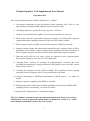
New Features Implemented in Ultimate Equalizer 9.0 – Digital
1. All internal calculations are now performed in linear frequency scale. This is a very
large change and includes HBT running in linear-frequency mode.
2. All displayed plots are presented in Log-Log scale – as before.
3. Program is streamlined and is lighter. Several unused options were removed.
4. MLS system operates at maximum frequency resolution of 262144 MLS sequence
length and has three sampling frequencies only: 44.1kHz, 48kHz, 96kHz.
5. Phase response used by all DSP sections of the program is HBT-derived only.
6. Impulse response design and optimization functionality now includes display of IR in
logarithmic scale with pre- and post-masker limits, and allows for final convolution of
filter’s impulse response with driver itself to obtain full channel impulse response.
7. Data and project files are very large, as they are required to store frequency/phase
data in linear frequency scale, up to 131072 data points.
8. “Guiding Filter” method for assisting in minimum-phase extraction has been
facilitated by introducing a copying function for SPL/phase curves from MLS system
and selection of filters.
9. Currently, the 8-partition version of UE is available. The 16-partition version, running
internally in linear frequency scale is being considered in the future.
10. Complex Smoothing of SPL/Phase implemented in MLS system – see inside for
details.
11. Impulse response resampling from 48kHz to 44.1kHz.
12. MLS measurements conducted with 96kHz sampling can be used with 48kHz DSP
sampling without re-measuring - see inside for details.
13. Dynamic SPL adjustments for 12 nominated outputs.
This User Manual is intended to provide information about new features in version 9,
and should be read in conjunction with the full User Manual for version 5, 6, 7 and 8,
and available from Bodzio Software Pty. Ltd. website.
1
Linear Frequency Scale for All Internal MLS / DSP Processes
Loudspeaker design is typically performed in logarithmic frequency scale, the LogLog scale, and is very well suited to the way we perceive sounds and music.
Starting with the measurement process, as soon as the impulse response is collected
and FFT applied, the resulting SPL and phase are calculated (mapped onto) logarithmic
frequency scale. From then onwards, driver equalization, all crossover design functions,
impedance compensation, and so on, are performed and visualized in the Log-Log frequency
scale.
Even the HBT algorithm was operating in logarithmic frequency scale and was fitting
very well into the design process. Obviously after all DSP functions, like driver equalization
and room corrections, were derived, there was a need to re-map the results back into the
linear frequency scale, so that partitioned convolution could operate properly at evenly
spaced frequency samples. This scheme worked well, undisturbed for a long time. Major
benefits were:
1. Small data files. Typically, 2000-3000 data points on the 20Hz-20kHz logarithmic
frequency scale provide sufficient accuracy and resolution for all design work.
2. Independent sampling frequencies for the measurement system and DSP playback.
This is because the re-mapping of the frequency scales provided convenient buffer
between the MLS and DSP. This is an important factor, providing a great deal of
convenience. Driver measurement files containing SPL/Phase data could be shared
with no restrictions, as the frequency re-mapping functionality always provided
reasonable recovery of the frequency and phase responses needed for the CAD
systems.
However, recently, Bodzio Software has been probing into the impulse response
performance issues, including plotting the amplitude of the final impulse response of a
channel in decibels. This allowed the visualization of the noise-level performance of the
impulse response. Several impulse responses of simple filters, generated initially in
logarithmic frequency scale and then mapped onto linear frequency scale have been collected
and then compared those with filters generated directly in linear frequency scale. The baselevel noise around the peak of the impulse response was always lower in linear frequency
scale by as much as 50dB. Noise of HBT-derived EQ filters + measured loudspeakers was
also lower in linear frequency scale by 10-15dB.
As a result of these findings, the Ultimate Equalizer program was to re-written, and a
linear frequency scale is now being used for all MLS and DSP functions, from start to finish,
while re-mapping into logarithmic scale only for the purpose of providing standard display of
all curves in Log-Log scale.
This is completely the opposite to what the previous approach was. Obviously, some
of the benefits of the original scheme are lost – data files are very large, and since the
frequency re-mapping is no longer there, the MLS system must run at the same sampling
frequency as the DSP system. Next, the HBT algorithm had to be re-written to operate in
linear frequency scale, so now, there are two versions of HBT. We can now compare the
impulse responses of filters with and without frequency re-mapping.
2
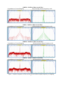
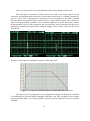
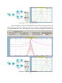
1000Hz, +24dB/oct Butterworth filter
Logarithmic-to-Linear Mapping
All processing in linear frequency scale
100Hz, +24dB/oct Butterworth filter
Logarithmic-to-Linear Mapping
All processing in linear frequency scale
5000Hz, +48dB/oct Butterworth filter
Logarithmic-to-Linear Mapping
All processing in linear frequency scale
5000Hz, -48dB/oct Butterworth filter
Logarithmic-to-Linear Mapping
All processing in linear frequency scale
Figure 1. Impulse responses of filters with (left) and without (right) frequency re-mapping.
3
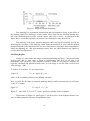
Figure 1 demonstrates, that the artefacts of frequency re-mapping algorithm result in
increased base-level noise around impulse response. This noise level is at -100dB, so it is
unlikely, that it would deteriorate normal-to-loud listening experience to any degree. I have
been using Ultimate Equalizer software for four years now, and the listening experience has
been outstanding. However, if there was a way to eliminate this issue, it would be worth to
pursue. And it turned out that there is a way to do it.
A complete elimination of frequency mapping and remapping of the data from the
signal processing path provides the most consistent way of generating final channel impulse
responses. The new signal processing path starts with the measurement system.
1. MLS measurement system operates in linear frequency scale, as usual.
2. Next, the FFT (also linear frequency scale) provides SPL and Phase of the measured
system.
3. SPL/Phase smoothing (traditionally performed and the SPL/Phase in logarithmic
frequency scale, as fractions of a dB) now has to operate on the FFT data in linear
frequency scale. Therefore Complex Smoothing was introduced – more on this later.
4. New HBT algorithm operates in linear frequency scale.
5. Loudspeaker equalization is performed in linear frequency scale.
6. Room correction is performed in linear frequency scale.
7. Filter generation and design is performed in linear frequency scale.
8. Finally, partitioned convolution is obviously performed in linear frequency scale.
So this is how the internal mathematics is now working. From the user’s perspective,
all plots and graphs are generated by remapping the data linearly processed in each and every
stage onto the standard Log-Log scale. Therefore, there is basically very little visual
difference between the older versions of the program and the latest, linear-scale version.
All the above changes have far reaching consequences. If the frequency re-mapping is
to be completely removed from the data and signal processing path, then we must maintain
the same sampling rate of the data from the measurement right down to the final partitioned
convolution stage.
This approach also requires, that measurements are made at the same sampling
frequency as the partitioned convolution will be run. So, for instance, if you intend to use the
playback function for WAV files at 44.1kHz, then you need to provide SPL/Phase data
measured by MLS system at 44.1kHz to start with. Or, if your goal is to run 96kHz Hi-Res
WAV files, then your measured SPL/Phase needs to be sampled at 96kHz.
The recommended measurement approach for collecting the impulse responses is as
follows:
1. Measure the driver using sampling frequency of 44.1kHz and SAVE the impulse
response into a file.
2. Then simply repeat the measurement instantly at 48kHz and SAVE the impulse
response into a file.
3. Finally repeat the measurement instantly at 96kHz and SAVE the impulse response
into a file.
4
It cannot be stressed enough, that the above approach is the best way to protect your
valuable measurement efforts and collected information for all future combinations of
sampling frequencies and buffer sizes used. It is recommended to label your Project Files,
embedding the sampling frequency into the file name.
Fortunately, the way the MLS system is operating, it allows you to use impulse
response collected at 96kHz for your 48kHz design and playback needs. So at the end of the
day, one needs to measure only at two sample frequencies: 96kHz and 44.1kHz.
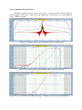
Impulse responses measured at those two frequencies can now be processed with 4
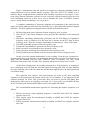
different low-frequency resolutions, depending on the selected UE buffer size. The room EQ
example shown below, illustrates how the low-frequency resolution is affected by selecting
different buffer sizes.
48kHz sampling frequency
512 Buffer – 11.72Hz bass resolution
1024 Buffer – 5.86Hz bass resolution
2048 Buffer – 2.93Hz bass resolution
4096 Buffer – 1.46Hz bass resolution
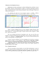
Figure 2. Room EQ affected by low-frequency resolution.
It is observable, that 11.72Hz bass resolution is not sufficient to activate excess group
delay detector necessary for room equalization to operate. The 2.93Hz resolution is accurate
enough to resolve where the non-minimum phase regions are. However, you could use the
2.93Hz bass resolution to detect, and exclude those regions from EQ, but still run your
system at lower bass resolution of 5.86Hz. The dependency of the bass resolution on the
buffer size has been highlighted before in previous UE manuals. UE system latency is the
other affecting factor, if you intend to use the software as a DSP processor for watching
visual media.
5
In general there are following latency options:
36ms – MP, UE Buffer = 512, Delta Buffer = 64, Lynx Buffer = 128, UE = 8P
75ms – LP, UE Buffer = 512, Delta Buffer = 64, Lynx Buffer = 128, UE = 8P
65ms – MP, UE Buffer = 1024, Delta Buffer = 128, Lynx Buffer = 128, UE = 8P
147ms – LP, UE Buffer = 1024, Delta Buffer = 128, Lynx Buffer = 128, UE = 8P
130ms – MP, UE Buffer = 2048, Delta Buffer = 128, Lynx Buffer = 256, UE = 8P
295ms – LP, UE Buffer = 2048, Delta Buffer = 128, Lynx Buffer = 256, UE = 8P
When equalizing 5.1HT or 7.1HT system, one needs to observe maximum tolerable
audio-video latency, which is 185ms. It is therefore observable, that a number of system
configurations listed above, will lead to a significantly lower latency than the 185ms
threshold. The following two examples clarify further the need to select latency-bass balance,
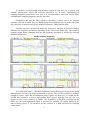
suitable for your needs. The first example illustrates the impulse response and SPL
performance of a 50Hz, +24dB/oct filter implemented with difference buffer sizes.
512 Buffer
2048 Buffer
50Hz, +24dB/oct Butterworth Filter
1024 Buffer
4096 Buffer
Figure 3. Impulse response and SPL performance of 50Hz, +24dB/oct filter.
The next example shows equalization implementation of a large, 18” subwoofer. This
is where the bass resolution is of importance.
6
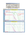
Example of Equalizing 18” Subwoofer
The subwoofer was measured using the in-built MLS system, and the impulse
response is shown below.
Figure 4. Subwoofer impulse response
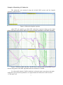
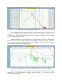
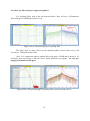
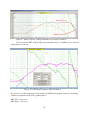
After FFT was applied, we obtain SPL and phase responses shown on the figure
below. The figure also presents HBT curves derived using logarithmic-scale HBT algorithm.
Figure 5. Measured SPL and phase, but the figure (bottom) also presents HBT curves
derived using linear-scale HBT algorithm and bass resolution of 5.86Hz.
It is observable, that the 5.86Hz resolution is obviously quite coarse, but seems quite
sufficient to proceed with equalization, as it approximates the subwoofer’s SPL down to
11.7Hz quite well.
7
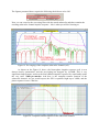
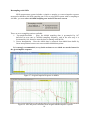
Figure 6. HBT parameters for the subwoofer.
Buffer 1024
Buffer 4096
Figure 7. SPL of all relevant EQ curves for two buffer sizes: 1024 and 4096
8
Complex Smoothing
Traditional smoothing applied to SPL and Phase curves involves “fractional octave
smoothing”, like 1/12oct or 1/6oct and so on. The smoothing is performed in logarithmic
frequency scale, and is easily applied to SPL curve and significantly more difficult to phase
response curve.
However, now the SPL/Phase data never makes it to the logarithmic scale for
processing, therefore the smoothing needs to be applied differently. The example below
shows an impulse response of a tweeter driver.
Figure 8. Impulse response of a tweeter driver
In the next step, FFT is applied to ultimately obtain SPL and phase responses.
However, the immediate result of the FFT is the driver’s complex Transfer Function,
expressed as TF(jw) = {Re(w)} + j{Im(w)}. The real and imaginary parts do not even
resemble the final SPL and phase curves yet, but are quite good candidates for smoothing.
Such operation is depicted on the figure below, where all relevant variables are
plotted in linear frequency scale. The smoothing algorithm must take into account, that at low
frequencies, data is very sparse, but at high frequencies, there is almost too much data. So the
frequency range over which the smoothing is calculated, has to be progressively expanded, as
the frequency increases.
Figure 9. Complex Smoothing explained.
9
The degree of smoothing is no longer expressed in “dB/oct”, but it offered as
“Level_1” to “Level_8” smoothing.
Figure 10. Final SPL/Phase with no smoothing
Figure 11. Final SPL with “Level 8” smoothing
As observable on the figures above, Complex Smoothing in linear frequency scale is
very effective in obtaining smooth SPL and phase curves. It is also very effective in removing
rapid phase fluctuations (+/-180deg), resulting in well-defined phase transitions, greatly
assisting in extracting the minimum-phase phase response. Combination of FFT windowing
and Complex Smoothing provides excellent results for SPL and phase smoothing.
It is recommended to apply FFT windowing to remove most of the time-of-flight
from the measurements before applying Complex Smoothing. This can be easily done by
correctly placing the FFT window.
10
Modelling of Pre-ringing in Impulse Response
Linear-Phase Mode of operation is the primary mode of operation of the Ultimate
Equalizer. Since the impulse response of a linear-phase system is symmetrical, it is therefore
recommended to inspect impulse response pre- and post-ringing levels. The inspection is
carried out using controls of the “Optimize / Export Impulse response” dialogue box – as
shown below.
Figure 12. Controls for estimating pre-ringing.
Before we examine impulse response characteristics, it is beneficial to highlight two
important factors associated with hearing the sound: pre-masking and post-masking
Source: http://zone.ni.com/reference/en-XX/help/373398B-01/svaconcepts/svtimemask/
Time (Temporal) Masking
“….Simultaneous masking describes the effect when the masked signal and the masking
signal occur at the same time. Human hearing is sensitive to the temporal structure of sound,
and masking also can occur between sounds that are not present simultaneously.
Pre-masking is when the test tone occurs before the masking sound. Post-masking is when
the test tone occurs after the masking sound. The following figure shows the time regions of
pre-masking, simultaneous masking, and post-masking in relation to the masking signal.
11
Figure 13. Slopes of temporal masking
Post-masking is a pronounced phenomenon that corresponds to decay in the effect of
the masking signal. Pre-masking is a more subtle effect caused by the fact that hearing does
not occur instantaneously because sounds require some time to sense. As indicated in the
figure above, researchers typically can measure pre-masking for only about 20 ms.
Post-masking is the more dominant temporal effect and can be measured for 100 ms
following the cessation of the masking sound. Both the threshold in quiet and the masked
threshold depend on the duration of the test tone. Researchers must know these dependencies
when investigating pre- and post-masking because they use short-duration test signals to
perform these measurements….”.
Modelling Regime
Firstly, it is observable, that slopes of temporal masking in Figure 13 are plotted using
lin-log scale, that is, time scale is linear in milliseconds, and level of test tone is in
logarithmic scale (decibels). Since impulse responses, which we are going to examine, are
typically calculated and plotted in linear scale, it is necessary to use the same vertical scale
units and type – dBs.
Y decibels of a variable “X” are expressed as:
Figure 14
Y = A * log10( X ) + B
where A, B are suitably chosen screen display constants.
Now, in order for the slope of temporal masking display similar characteristics as on Figure
1, the “X” variable
Figure 15
X = exp(-T / C ) + D
Where T = time from T=T1 to T=T2, and C and D are suitably chosen constants.
Expressions on Figure 14 and Figure 15 can be used to create temporal masks if we
were to display impulse responses in logarithmic scale.
12
Calibration of the Simulation Process
Mathematical formulas describing pre- and post-masking slopes on Figure 13 were
not available. Therefore, visual inspection of Figure 13 resulted in adjusting coefficients
A,B,C and D to obtain plots of both maskers, similar to the ones on Figure 13 (green curve on
Figure 16-right). Please note, that pre-and post-masking is shown from 0dB to 50dB on the
vertical scale on Figure 13.
For calibrating the peak level of the impulse response, a 1000Hz, +12dB/oct
Butterworth filter was used, and the corresponding impulse response is shown below.
Figure 16. Calibrating Simulation Process for IR.
Figure 16 depicts calibration process for this simulation. Impulse Response (IR)
(green curve) is plotted with 10dB/div horizontal scale resolution. IR of such system has a
peak at 0dB level – see green peak at Figure 16-right. The floor of IR is clipped at -170dB
level – observe no noise at all.
IR is now calculated and shown in logarithmic scale. Also, since the IR can be
negative as it wiggles along the time scale, the negative values are shown as absolute values
of the IR. (in C-language: Y = 20log10(fabs(IR)) ). This is why the IR looks differently from
what you would typically see in MLS systems.
In order to increase confidence level in the simulation, the levels the pre- and postmasker shown on Figure 13 were dropepd by -20dB. The new, much more stringent
masker levels are now plotted in pink on Figure 16-right, and are extended down to
-70dB range. From now onwards, the gain in the system must be kept constant
for all impulse responses. We will now proceed to inspect several impulse responses for
potential audibility of pre-ringing.
Case 1. Equalized subwoofer.
Since the pre-masker and post-masker are time-limited phenomenon, it may be
prudent to examine the slowest and heaviest driver in the system – the subwoofer. The driver
in this example is really big, 18” McCauley subwoofer, mounted in a 300 litre venter
enclosure. The equalization and filtering transfer function is depicted on the figure below.
13
Figure 17. Correction filter for subwoofer.
It is noticeable, that the phase response of the correction filter is inverse. This is
because we are developing a linear-phase subwoofer. Also, the correction characteristics are
evident below 340Hz, as the filter transfer function (-24dB/oct, LR filter) is also correcting
driver’s SPL/phase below 340Hz.
Impulse response of the correction filter is shown below on Figure 18. Please note,
that the filter alone has developed significant pre-ringing and clearly fails the -70dB premasker level. It is also observable, that the impulse response is very asymmetrical, not what
you would expect from a linear-phase system.
Figure 18. Impulse response of the correction filter (green) in decibels, 10dB/div.
This is a very common misconception, when discussing linear-phase filters. Simply
because this is NOT the subwoofer channel impulse response – it’s missing the actual
subwoofer transfer function.
14
The figures presented above require the following check-boxes to be ON.
Now, we can convolve the correcting filter with the actual subwoofer and then examine the
resulting subwoofer channel impulse response – this is what you will be listening to.
Figure 19. Pre-ringing of the complete subwoofer channel (red).
As shown on the Figure 19 above, the linear-phase impulse response (red) is now
almost exactly symmetrical, and the pre-ringing has dropped by 10-20dB. This is very
significant improvement, and now the total channel impulse response fits comfortably under
the very strict -70dB pre-masker. And here is the complete transfer function of the
subwoofer channel. As you would expect, the SPL is equalized right up to 340Hz, and the
phase response is now a flat line.
Figure 20. Complete transfer function of the subwoofer channel.
15
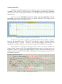
Next, we can perform some measurements on the newly equalized subwoofer.
2ms-wide pulses separated by 350ms space were used as the source signal. On the
2ms pulse, the minimum-phase subwoofer version delivered a more of a “thump” instead of a
pop or a click. This is perhaps not surprising, as the post-ringing of the pulse extended
to130ms and far exceeded the 30ms “memory effect” of the auditory system. Here, the driver,
filter and vented enclosure added it’s own, combined signature. It is also observable, that the
minimum-phase version of the subwoofer has converted the clearly asymmetrical pulse into a
much more symmetrical bi-polar pulse with post-ringing. This is clearly visible on the screen
shots below.
Figure 21. 2ms Impulse in Linear-Phase Mode
and
Minimum-Phase Mode
And here is the frequency and phase responses of the subwoofer.
Figure 22. Frequency and phase responses of the equalized subwoofer.
The above level of performance was accomplished with the low-frequency resolution
of 5.86Hz (Buffer 1024 and 48kHz sampling). When the “raw” SPL and phase do not contain
rapid peaks and valleys, it is clearly possible to equalize the low-frequency driver to excellent
standard.
16
Case 2. Equalized Tweeter driver
Impulse responses: the green curve is the same – tweeter measured and processed in
linear frequency scale. Red – with convolved loudspeaker. All curves fit very well under the
strict, -70dB pre-masker.
Figure 23. Impulse response of the complete tweeter channel (red).
Figure 24. Correcting filter, again with the phase response inverted
Figure 25. Tweeter channel SPL/Phase response – flat phase response and equalized driver.
17
Are there any filters that pre-ring unacceptably?.
Yes, peaking filters, such as the one depicted below. Here we have a Q-Parametric
filter with gain of 30dB and Q-factor of 10.
Figure 26.Pre- and post-ringing of a peaking filter.
This filter rings so much, that even the minimum-phase version (blue curve) will
exceed our -70dB post-masker limit.
Also, if we implement again a peaking filter with gain of 30dB and Q-factor of 10,
and hope, that convolving it with the driver would eliminate pre-ringing – no, the preringing will manifest itself again.
Figure 26.Pre- and post-ringing of a peaking filter convolved with a driver.
18
Resampling to 44.1kHz
MLS measurement system includes a simple re-sampler, to convert impulse response
measured at 48kHz to 44.1kHz sampling rate. Prior to using MLS system with re-sampling to
44.1kHz, you must select 44.1kHz sampling rate in the Preferences screen.
There are two resampling options available:
1. Up-sample/Decimate – Here, the 48000 sampling data is up-sampled by 147
therefore in now runs at 7056000 sampling frequency, and in the next step it is
decimated by 160, therefore now the data is running at 44100 Hz.
2. Linear Interpolation – Here the 44100 data is extracted from 48000 data buffer by
linear interpolation between two most suitable 48000 data points.
It is strongly recommended, to try both variants to see which one works better for
the given impulse response.
Figure 27. Original Impulse Response in 48kHz
Figure 29. SPL and phase calculated from original 48kHz impulse response
19
Figure 30. The same impulse response after resampling to 44.1kHz
Figure 31. SPL and phase calculated from the re-sampled 44.1kHz impulse response
Figure 32. Resampling Decimation (red) vs. Linear Interpolation (beige)
20
Copying function for SPL/phase curves from MLS system and filters
The copying function primarily is designed to assist in developing minimum-phase
phase response of the measured driver in MLS system.
Dome tweeter example
In this example we will examine minimum-phase response of a popular Hi-Fi dome
tweeter driver.
The dual-channel MLS system is actually designed to provide minimum-phase
response of the measured driver, within the error of +/- one sample time. Here is how it
works.
When the loop test is performed, you will notice, that you will get flat phase response
of the signal channel when you place the start of the FFT window at 10 samples before the
peak of the impulse response – why?. This is because the reference channel is also
automatically windowed with the fixed start of the FFT window also at 10 samples in front of
the IR start. The loop test simply measured the true “minimum-phase” phase response of the
sound card. However, each PC MLS system must be examined individually for the Reference
Impulse response first.
Reference Impulse Response:
Peak of 41463 at bin=60
Peak -1 of 8584 at bin 59.
Peak - 2 of -3762 at bin 58,
the IR has gone large negative now. For this system, bin 59 is the start of the impulse
response.
Therefore, the start of the FFT window for the Reference impulse response is 10
sample times from the peak, or 9 sample times from the start of the impulse response.
Now, we can apply the same technique to the loudspeaker measurement, and place the
start of the FFT window 9 samples ahead of the start of the IR – and we’ll obtain minimumphase phase response of the loudspeaker straight away, with +/- one sample time error. To
eliminate this small uncertainty error, we have to add/subtract small delay (or manipulate
HBT slopes) to get the measured and HBT calculated phase into alignment.
It is important to determine the start of the impulse response (not the peak), as various
drivers have different rising slopes of the impulse response, therefore the peak will be located
at various distances from the start of the impulse. So, first we need to find the peak of the
impulse response:
the peak is In = 1886.90,
located at Bin=339
21
Next we move the cursor to the left of the impulse response, one sample time, and each time
we monitor the “In” vale.
the In = 4.94 and is very close
to zero, therefore, we determine that the start of the impulse response is Bin = 336.
Finally, we need to move the start of the FFT window 9 sample times (for this system it is 9
sample times) to the left from the start of the impulse response, 336-9 = 327.
Now, the start of our FFT window is located at Bin = 327. See figure below.
Figure 33. Start of the FFT window (9 bins to the left).
Next, we need to obtain the SPL and phase of the driver using FFT. And here is the result.
Figure 34. Resulting SPL and phase responses.
To increase the level of confidence on the phase response, it is desirable to overlap
band-pass filter SPL/phase responses, comparable with the loudspeaker amplitude response.
This will provide us with filter’s phase response, which one would use as an additional
guidance for the locations of the 360deg transitions of the filter and the measured phase –
they should be very close.
22
Since this is a tweeter example, and we are only interested in finding the highfrequency tail, then a simple low-pass filter located at 27kHz with -48dB/oct slope can be
used. It is observable, that the slope of the filter is slightly slower than the measured
response, so we assume -51dB/oct as the asymptotic slope of the measured driver SPL. Also,
the 360deg transitions of both: filter and the measured SPL are very close.
Figure 35. Calibration File simulator used as filter generator.
Now, position mouse pointer exactly on the SPL curve in the “Mike + Preamp” TAB
and press left mouse button. The SPL curve will be highlighted in pink colour and the SPL
and phase curves will be copied into “Overlapped Curves” TAB.
Next, position mouse pointer again exactly on the SPL curve in the “SPL + Phase”
TAB and press left mouse button. The SPL curve will be highlighted in pink colour and the
SPL and phase curves will be copied into “Overlapped Curves” TAB.
Figure 36. SPL of the driver and filter SPL highlighted in pink.
Examining the phase response of the filter and measured driver, and particularly the
360deg phase transition, it is evident, that in order to get the measured phase response phase
response 360deg transition to overlap filter’s phase transition, a small, 12usec delay needs to
be added to the phase response of the measured SPL curve.
23
Figure 37. Phase response 360deg transitions now overlap accurately.
We can now run HBT with the high side asymptotic slope of 51dB/oct, to see how the
whole picture works out.
Figure 38. Final linear-frequency HBT calculated.
We observe a perfect alignment of measured and HBT-derived phase responses assuming 51dB/oct asymptotic slope of the “guiding filter”.
HBT SPL – blue curve
HBT Phase – red curve
24
General workflow and data flow
It will pay dividends if you plan ahead and determine upfront, what is the UE going to
be used for. The purpose of this is to determine what sampling rates will be necessary in the
future usage of the program. Also, there is the issue of latency, and therefore the size of UE
Buffer (512, 1024, 2048 and 4096) and corresponding bass resolution. If you are unable to
make this determination, the safest option is to perform full set of measurements. Complete
elimination of the re-mapping of the frequency scales in the data and DSP processing results
in some additional workload. This could be summarized as follows:
1. Measure drivers at all three sampling rates: 44.1kHz, 48kHz and 96kHz. This is not a
significant requirement, because all that needs to be done is to set the sampling
frequency to the next value and repeat the measurement. Please SAVE each impulse
response as you go, and clearly mark what is the sampling frequency in this impulse
response file. As a safety feature, the impulse response file actually saves the
sampling frequency as well. The IR files will be reused several times.
2. In the next step, you would create driver’s data file. Once again, the description here
presents all options included.
First, go to Preferences screen and set the size of the buffer – choose from 512, 1024,
2048 or 4096 size. This will determine the bass resolution and latency.
Also select the sampling rate, which must be the same as the sampling rate of the
impulse response you saved previously.
Go to MLS system and load driver’s impulse response. Now you should have the
MLS system at the same frequency as the DSP section.
Next, determine the windowing, complex smoothing, and extra dBs to be added and
run the FFT. The resulting SPL and phase should be smooth and phase should not
contain any spurious transitions.
Next, go to “File Editor” screen and set the HBT parameters. You will notice, that
there are two versions of HBT: linear frequency HBT and logarithmic frequency
HBT. The reason for this is, that logarithmic frequency HBT (3100 bins) calculates
much faster than linear frequency HBT ( up to 65536 bins), so you can use
logarithmic frequency HBT to play with the HBT settings, but once you are happy
with those, you MUST use linear frequency HBT. Only the SPL/Phase data calculated
via linear frequency HBT is saved to driver’s data file.
IMPORTANT: Save the driver’s file, clearly marking the buffer size and
sampling frequency in the driver file name.
The above description applies to measurements not requiring multiple impulse
responses to be saved. Woofers for example, will require port and cone close-mike
measurements and then 1m distance SPL measurements. ALL of those must be
conducted at three sampling rates. Then you need to combine relevant impulse
responses and create all required driver files.
25
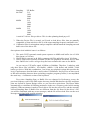
Sampling
44.1kHz
UE Buffer
512
1024
2048
4096
48kHz
512
1024
2048
4096
96kHz
512
1024
2048
4096
A total of 12 driver files per driver. This is when planning ahead pays off.
3. When the Project File is created, you’ll need to load driver files, that are mutually
compatible, so that each driver file is of the same sampling frequency and buffer size.
4. Calibration files for microphone and pre-amplifier should match the sampling rate and
buffer size of the driver file.
One option to deal with this issues is as follows:
1. The main 5.2HT surround sound system operates at 48kHz and buffer size of 1024
bins (latency of 147ms).
2. WAVE Player operates at 44.1kHz ( commercial CDs) and buffer size of 1024 bins.
3. WAVE Player also operates at 96kHz (Hi-Res file playback) and buffer size of 2048
bins. Buffer size is twice as big to keep the bass resolution the same as for 48kHz.
As you can see, UE buffer equals 1024bins or 2048bins. Therefore, I ended up with
only three driver files (44.1kHz / 1024 buffer), (48kHz / 1024 buffer) and (96kHz / 2048
buffer) per driver. With this combination, I can create any playback system that provides the
level of performance described above and in other UE Manuals. Project Files are then saved
to HD and switching between them (switching complete program profiles) is accomplished
the usual way – via numeric section of the keyboard.
Every time Sampling Rate or Buffer Size are changed in Preferences screen, the
previous frequency scale of the DSP engine becomes invalid and therefore the SPL and phase
plots are cleared in System Design screen, so you’ll need to replot them. The Player Mode
automatically re-calculates all filtering parameters in the new frequency scale before starting
playback. When an attempt is made to load a driver file into the project file, and the currently
selected Sampling Rate or Buffer Size are different from the one stored in the driver’s file,
you will be confronted with one or two messages, and the file will not load. Here are the error
messages associated with possible mistakes.
26
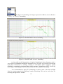
Phase response used by DSP section is HBT-derived
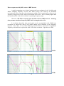
A quick comparison (see below) between the bass resolution for all 4 buffers and
48kHz sampling frequency reveals, that HBT process will clean-up all unwanted
environmental noise crept into the measurement results. This is particularly evident in the
frequency range below 10Hz, where the measured SPL level at 1Hz is actually higher than
the maximum SPL of the driver within it’s operating frequency range.
Therefore, SPL/Phase response used by DSP section is HBT-derived – meaning,
that you must run linear frequency HBT before saving the driver file.
It is clearly observable, that good results can be accomplished with 5.86Hz bass
resolution for subwoofers, that do not exhibit unduly rapid variations in the frequency
response. Also, there is very little difference between drivers processed in logarithmic
frequency scale and drivers processed with 1.47Hz bass resolution – right down to 10Hz.
5.86Hz
2.93Hz
27
1.47Hz
LOG
Figure 39. Comparison between the bass resolution for all 4 buffers and 48kHz
sampling frequency.
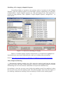
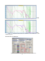
Real-time SPL level adjustments
Figure 40. Preferences screen with outputs selectable for adjustments.
28
Important Note: When you first open the Preferences screen, the residual data displayed in
these four fields may contain random value. Please assign your output ports to these data
fields immediately.
Adjusting Master Volume
Master Volume control is performed remotely by pressing ARROW UP/DOWN
keyboard keys. The SPL steps in 3dB increments/decrements.
Adjusting Volume of 4 Nominated Drivers (Rear Speakers)
This is a very handy and often used feature. It appears, that rear loudspeakers are not
mastered in the recording studios at the same level. Thus some movies/concerts are lacking
the sound coming from the rear speakers, and others are correctly edited. To remedy this
problem, UE allows you to nominate 4 output ports (these will be your 4 drivers in the rear
speakers) in the Preferences screen – see example below.
Adjusting Volume of 4 Nominated Drivers (Subwoofers)
29
Adjusting the BBM levels
This adjustment control the level of low-frequency (filtered from all-left channels and
all-right channels) signal mixed into left and right subwoofers.
Page Up = +2dB
Page Down = -2dB
Adjusting Volume of 4 Nominated Drivers (Front Tweeters)
This particular adjustment option came to being after auditioning many movies and
concerts. There seems to be a subtle difference (well, sometimes quite pronounced) in the
amount of treble recorded during the final studio mix. Some video material has excessive
brilliance and sibilance, and these can be controlled to large extent by controlling the level of
tweeters in front speakers.
Brilliance - The 6kHz to 16kHz range controls the brilliance and clarity of sounds.
Too much emphasis in this range can produce sibilance on the vocals.
Sibilant - "Essy" Exaggerated "s" and "sh" sounds in singing, caused by a rise in the
response around 6 to 10 kHz. Often heard on radio.
In order to be able to adjust those level during playback, you need to nominate the
outputs to which the tweeters are connected. In the example below these are: Out 1, Out 3
and Out 5. Output 7 is a dummy one, and nothing is connected to it.
The levels are controlled via “Home” and “End” keys on the keyboard in +/- 1dB
steps.
Home = Tweeters -1dB
End = Tweeters +1dB
30
Figure 41. Tweeter at +10dB
and tweeter at -10dB level.
Figure 42. Commonly used voicing with 6dB difference between 50Hz and 10kHz.
Summation of two impulse responses with time delay
Finally, a simulation of a typical 3-way system, where the crossover frequencies are
selected as 500Hz and 5000Hz. The filter if 24dB/oct LR design. The sampling rate is 48kHz,
and impulse responses are shown in decibels.
31
Simulating woofer / midrange section.
Woofer-midrange sections are simulated first in the CAD system design screen, and
after frequency responses are plotted, you can go to “Optimize / Export Impulse Response”
menu option and select “IR1 + IR2 Advanced” when you enter 40 samples for timing offset.
Simulating midrange / tweeter section.
32
Midrange-tweeter sections are simulated next in the CAD system design screen, and
after frequency responses are plotted, you can go to “Optimize / Export Impulse Response”
menu option and select “IR1 + IR2 Advanced” when you enter 40 samples for timing offset.
Time-of-flight distance difference between drivers is as follows:
woofer – midrange = 28.6cm = 40 samples @ 48kHz
midrange – tweeter = 28.6cm = 40 samples @ 48kHz.
Interestingly, the short analysis above indicates, that midrange and tweeter will have
less margin (well, almost none) under the stringent -70dB pre-masker.
Data Files Compatibility
Due to introduction of the linear frequency scale in data files, the files have become
very large, as the must hold 65536 data points for 8-partition version and anticipated 131072
data points for 16-partition version of the software.
Driver files are now 4.1Mb and Project files are almost 600Mb in size. The new data
files are not compatible with older versions of the program.
33