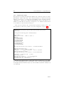
Download Shoot-1.1 Package - User Guide

Shoot-1.1 Package - User Guide
Pierre Martinon, Joseph Gergaud
To cite this version:
Pierre Martinon, Joseph Gergaud. Shoot-1.1 Package - User Guide. [Technical Report] RT0354, 2008, pp.41. <inria-00287879v1>
HAL Id: inria-00287879
https://hal.inria.fr/inria-00287879v1
Submitted on 15 Jul 2008 (v1), last revised 2 Jan 2008 (v2)
HAL is a multi-disciplinary open access
archive for the deposit and dissemination of scientific research documents, whether they are published or not. The documents may come from
teaching and research institutions in France or
abroad, or from public or private research centers.
L’archive ouverte pluridisciplinaire HAL, est
destin´ee au d´epˆot et `a la diffusion de documents
scientifiques de niveau recherche, publi´es ou non,
´emanant des ´etablissements d’enseignement et de
recherche fran¸cais ou ´etrangers, des laboratoires
publics ou priv´es.
INSTITUT NATIONAL DE RECHERCHE EN INFORMATIQUE ET EN AUTOMATIQUE
Shoot-1.1 Package - User Guide
Pierre Martinon — Joseph Gergaud
N° ????
Juin 2008
ISSN 0249-0803
apport
technique
ISRN INRIA/RT--????--FR+ENG
Thème NUM
Shoot-1.1 Package - User Guide
Pierre Martinon∗ , Joseph Gergaud†
Th`eme NUM — Syst`emes num´eriques
´
Equipes-Projets
Commands
Rapport technique n➦ ???? — Juin 2008 — 35 pages
Abstract: This package implements a shooting method for solving boundary
value problems, for instance resulting of the application of Pontryagin’s Minimum Principle to an optimal control problem. The software is mostly Fortran90,
with some third party Fortran77 codes for the numerical integration and nonlinear equations system. Its features include the handling of right hand side
discontinuities (such as caused by a bang-bang control) for the integration of
the trajectory and the computation of Jacobians for the shooting method. The
particular case of singular arcs for optimal control problems is also addressed.
Key-words: Boundary value problem, discontinuous right hand side, optimal
control, shooting method, singular arcs
∗
†
INRIA-Saclay and CMAP UMR CNRS 7641, Ecole Polytechnique, 91128 Palaiseau
Universit´
e de Toulouse, INP-ENSEEIHT-IRIT, team APO
Centre de recherche INRIA Saclay – Île-de-France
Parc Orsay Université
4, rue Jacques Monod, 91893 ORSAY Cedex
Téléphone : +33 1 72 92 59 00
Package Shoot-1.1 - Guide Utilisateur
R´
esum´
e : Ce paquetage impl´emente une m´ethode de tir pour la r´esolution de
probl`emes aux deux bouts, tels que ceux obtenus par application du Principe
du Minimum de Pontryaguine `a un probl`eme de contrˆole optimal. Le logiciel
est principalement ´ecrit en Fortran90, et utilise des codes externes en Fortran77
pour l’int´egration num´erique et la r´esolution de syst`emes non lin´eaires.Il prend
notamment en compte les discontinuit´es du second membre, du point de vue de
l’int´egration de la trajectoire ainsi que du calcul de Jacobien pour la m´ethode de
tir. Le cas particulier des arcs singuliers pour les probl`emes de contrˆole optimal
est ´egalement trait´e.
Mots-cl´
es : Probl`eme aux deux bouts, second membre discontinu, contrˆole
optimal , m´ethode de tir, arcs singuliers
Shoot-1.1 Package - User Guide
3
Shoot package v1.1 - User Guide
P. Martinon1 , J. Gergaud2
06/2008
1 Research
scientist, INRIA FUTURS, team COMMANDS, pierre.martinon@inria.fr
Professor, Universit´
e de Toulouse, INP-ENSEEIHT-IRIT, team APO,
joseph.gergaud@enseeiht.fr
2 Assistant
RT n➦ 0123456789
4
Pierre Martinon , Joseph Gergaud
Contents
1 Introduction
1.1 Shooting method . . . . . . . . . . . . . . . . . . . . . . . . . . .
1.2 Continuation . . . . . . . . . . . . . . . . . . . . . . . . . . . . .
5
5
7
2 Using the Shoot package
2.1 Package overview . . . . . . . . . . . . . . . . . . . . . . . . . . .
2.2 User supplied subroutines and input files . . . . . . . . . . . . . .
8
8
10
3 Discontinuities handling
16
3.1 Switchings detection . . . . . . . . . . . . . . . . . . . . . . . . . 16
3.2 Variational System . . . . . . . . . . . . . . . . . . . . . . . . . . 17
3.3 Sample problem: Orbital transfer . . . . . . . . . . . . . . . . . . 17
4 Singular arcs handling
21
4.1 Singular arcs and continuation . . . . . . . . . . . . . . . . . . . 21
4.2 Shooting problem formulation . . . . . . . . . . . . . . . . . . . . 22
4.3 Sample problem: Goddard (3D) . . . . . . . . . . . . . . . . . . . 23
5 Appendix: Files for the sample problems
28
5.1 Orbital transfer . . . . . . . . . . . . . . . . . . . . . . . . . . . . 28
5.2 Goddard problem . . . . . . . . . . . . . . . . . . . . . . . . . . . 30
INRIA
Shoot-1.1 Package - User Guide
1
5
Introduction
This package of Fortran 90 routines implements several variants of indirect
shooting methods for optimal control problems, with an embedded homotopy
approach (discrete continuation). Special care is given to the numerical integration of the shooting function and the precise computation of its Jacobian,
especially in the discontinuous case. Originally designed for the resolution of
bang-bang low thrust orbital transfers for the CNES3 , the software has been
since then extended to handle problems with singular arcs. The integration of
state constraints is currently under development.
1.1
Shooting method
We begin with a brief presentation of the single shooting method, which is part
of the indirect methods, and is based on Pontryagin’s Maximum Principle (we
refer readers interested in these methods to [17, 7, 2, 19] for instance). We recall
that direct methods, on the other hand, typically involve the partial (control)
or total (control and state) discretization of the problem, and then use various
approaches (SQP and interior point techniques for instance) to solve the resulting optimization problem. Direct methods are thus supposed to be robust, but
the counterpart is a relatively low precision, and a huge problem size depending
on the discretization stepsize used. This makes these methods ill-suited to some
particular cases, such as problems with a bang-bang control structure and a
huge number of commutations.
Back to the indirect methods, single shooting consists in finding a zero of the
shooting function associated with the original problem. There is no discretization, even if the method still involves an integration of the system in some way.
It is a fast and high precision method, but often requires a good initial guess:
as they typically consist in applying a (quasi-)Newton solver to the shooting
function, the convergence radius may be quite small, depending on the problem. This is particularly true for problems involving commutations, or worse,
singular arcs, and often leads to the use of continuation (homotopy) techniques
to obtain a suitable initial point.
We consider a general optimal control problem in the Bolza form

R tf
Objective

 M in g(t0 , x(t0 ), tf , x(tf )) + t0 l(t, x, u) dt


 x˙ = f (t, x, u)
Dynamics
(P )
u∈U
Admissible Controls



Initial Conditions
ψ0 (t0 , x(t0 )) = 0


ψ1 (tf , x(tf )) = 0
T erminal Conditions
Notation/Remark: for clarity, the time t will often be omitted in the formulas,
except in ambiguous cases.
We use here and in all the following the notations: x ∈ Rn for the state,
u ∈ Rm for the control, U the set of admissible controls, and f for the state
dynamics. We assume that the initial and final times t0 and tf are fixed. Free
3 The
French space agency
RT n➦ 0123456789
6
Pierre Martinon , Joseph Gergaud
final time problems can always be reformulated as fixed time problems using
the classical time transform t = s.tf with s ∈ [0, 1] the normalized time and tf
an additional state variable. We introduce the costate p, of same dimension as
the state x, and define the Hamiltonian by
H(t, x, p, u) = l(t, x, u) + (p|f (t, x, u)).
Remark: we thus assume in all the following that we are in the normal case,
meaning that the costate p0 associated to the integral objective l is non zero, and
can be made equal to 1, by dividing the whole costate p by p0 ...
Pontryagin’s Maximum Principle then states that, under the assumptions:
❼ ∃ (x, u) feasible for (P ), with x absolutely continuous and u measurable.
❼ f and l are continuous with respect to u and C 1 with respect to t and x.
❼ g, ψ0 , ψ1 are C 1 with respect to x.
Let (x, u) be an optimal pair for (P ), then
(i) ∃ p 6= 0 absolutely continuous such that we have the Hamiltonian system

∂H
 x˙ = ∂p (t, x, p, u)
 ˙
p = − ∂H
∂x (t, x, p, u)
(ii) u is solution of M inw∈U H(t, x, p, w) ae in [t0 , tf ].
(iii) “Transversality conditions”: ∃ (µ0 , µ1 ) such that

ψ0 (x(t0 )) = 0



∂Φ

 p(t0 ) = − ∂x0 (t0 , x(t0 ), tf , x(tf ), µ0 , µ1 )
(T C)


ψ1 (x(tf )) = 0



∂Φ
(t0 , x(t0 ), tf , x(tf ), µ0 , µ1 )
p(tf ) = ∂x
f
with
Φ : (t0 , x0 , tf , xf , µ0 , µ1 ) 7→ g(t0 , x0 , tf , xf ) + (ψ0 (t0 , x0 )|µ0 ) + (ψ1 (tf , xf )|µ1 )
Remark: this is why indirect methods are sometimes referred to as necessary
condition methods.
Now we denote y = (x, p) and ϕ the state-costate dynamics derived from
the Hamiltonian system. We assume here that the expression of the optimal
control given by the necessary conditions (Hamiltonian minimization) is actually
a function, noted γ, ie u(t) = ArgM inw∈U H(t, x, p, w) = γ(t, y). Solving (P ) is
equivalent to solving the following Boundary Value Problem

ae in [t0 , tf ]
 y˙ = ϕ(t, y, γ(t, y))
Boundary Conditions at t0
c0 (t0 , y(t0 )) = 0
(BV P )

c1 (tf , y(tf )) = 0
Boundary Conditions at tf
Note: these Boundary Conditions c0 and c1 correspond to the Transversality
Conditions mentioned above, that contain the Initial and Terminal conditions
INRIA
Shoot-1.1 Package - User Guide
7
of (P ) in addition to the constraints on the costate p.
It is possible to integrate y = (x, p) if we set the value of y(t0 ), and we then
obtain the following Initial Value Problem
y˙ = ϕ(t, y, γ(t, y))
ae in [t0 , tf ]
(IV P )
y(t0 ) = ζ
Initial V alue.
We introduce now an application called the shooting function, which basically maps the initial value ζ to the value of the Boundary conditions at tf
for the corresponding solution of (IV P ). In practice, the initial conditions ψ0
of the problem (P ) already give a part of y(t0 ), so the unknown of the shooting
function is reduced to the “missing” part, that we note z. A frequent situation
is when the initial conditions determine the initial state x(t0 ), therefore z is actually the initial costate p(t0 ). Then the value of the shooting function is given
by the boundary conditions at tf for the solution y(·, z) of (IV P ) corresponding
to the initial value y(t0 , z) = (x0 , z)
(Shooting f unction)
S : z 7→ c1 (y(tf , z)).
Finding a zero of the shooting function S is then equivalent to the resolution
of (BV P ), and therefore also gives a solution of (P ). The “shooting method”
thus consists in solving the equation S(z) = 0, as summarized below:
Problem
(P )
−→
Boundary Value
Problem (BV P )
−→
Initial Value Problem (IV P )
and Shooting function S
An interesting particular case is when the optimal control is discontinuous
and presents switchings (or commutations), for instance when the command law
is bang-bang. More precisely, the Hamiltonian minimization gives
u = γ1 (t, y)
u = γ2 (t, y)
u = Γ(t, y)
,
,
,
if ψ(t, y) < 0
if ψ(t, y) > 0
if ψ(t, y) = 0,
with Γ(t, y) a subset of U , and ψ the switching function, whose zeros correspond
to the commutations of the optimal control. We assume that the set of switching
times t such that ψ(t, y) = 0 is finite. We then obtain y(·, z) as solution of the
initial value problem with a discontinuous right hand side

, if ψ(t, y) < 0
= ϕ1 (t, y)
 y˙
y˙
= ϕ2 (t, y)
, if ψ(t, y) > 0,
(IV P )disc

y(t0 , z) = (x0 , z)
As mentioned earlier, one of the main practical difficulties for the shooting
method is to find a suitable initial point, due to the small convergence radius
of the newton method applied to the shooting function. In our case, we use a
continuation approach (homotopy), as described below.
1.2
Continuation
It is well known that shooting methods are quite sensible to the initial guess,
and it is often quite hard to achieve convergence for non trivial problems because of this. An interesting way to obtain a suitable starting point is to use
RT n➦ 0123456789
8
Pierre Martinon , Joseph Gergaud
continuation (or homotopy) approaches. The principle of continuation is to find
a certain homotopy that connects the original problem to an easier one, and
then to follow the zero path of this homotopy, from a solution of the easy problem to a solution of the original one.
In the following, we will often parametrize the original problem (P ) by a
certain λ ∈ [0, 1], and obtain a problem family (Pλ ) such that (P1 ) = (P ).
Moreover, we expect that we are able to find a solution of (P0 ). If we note Sλ
the shooting function associated to (Pλ ), we can define the homotopy
H : (z, λ) 7→ Sλ (z).
Assuming we know a zero z0 of H(·, 0) = S0 , all we have to do is to follow the
zero path of H from λ = 0 to λ = 1, at which point we have obtained a zero of
H(·, 1) = S1 = S, and therefore a solution of (P ).
There are several ways to perform this path following, such as PredictorCorrector methods (or differential homotopy) that treat the zero path as a
differentiable curve, Piecewise Linear (or simplicial) methods that build a PL
approximation of the path over a triangulation of the space. We refer the interested readers to [1] for a general overview of continuation methods, and [8] in
the context of Newton methods for nonlinear problems.
A more basic approach is just to try to solve a sequence of problems (Pλk ), k =
1, . . . , N such that λ0 = 0 and λN = 1, by using the solution found for (Pλk ) as
initial guess for (Pλk+1 ), or with a basic linear prediction step. The stepsize hk
for the homotopic parameter (such that λk+1 = λk + hk ) can be set to a certain
fixed value, or something a little more refined. For instance we can introduce
a tolerance tol on the norm of the shooting function that indicates a successful
convergence of the shooting method. Then we can start with a stepsize h0 = 1
and try to solve (P1 ) directly; if the attempt fails, we divide the stepsize hk
by 2, and try again, until we reach λ = 1. It is then safer to also stop the
continuation if a certain maximal number of iterations has been reached, or if
the stepsize hk goes below some minimal value. This method is implemented in
the Shoot package, and can be quite effective for well chosen homotopies.
2
2.1
Using the Shoot package
Package overview
Web page: http://www.cmap.polytechnique.fr/˜martinon/
Contact: pierre.martinon@inria.fr, joseph.gergaud@enseeiht.fr
All questions or comments about the Shoot package are welcome !
The Shoot package should contain the following files:
Core files
- ShootCont.f90 : discrete continuation module
- Shoot.f90 : shooting functions module
INRIA
Shoot-1.1 Package - User Guide
-
9
Integrators.f90 : integrators interface
RHS.f90 : IVP right hand side handling
Common.f90 : some common subroutines
ShootDefs.f90 : global variables
Makefile
Sample problem files
-
OrbitalFuns.f90 : orbital transfert with discontinuous control
FishingFuns.f90 : fishing problem with singular arcs
RegulatorFuns.f90 : quadratic regulator problem with singular arcs
GoddardFuns.f90 : 3D Goddard problem with singular arcs
Visualization scripts
- sol.m: Matlab script for solution visualization (use solorb.m for orbital transfer)
- contpath.m: Matlab script for continuation path visualization
Third party codes
❼ rkf45.f : Runge Kutta Fehlberg (4-5) integrator
L. Shampine, H. Watts,
http://netlib.org/ode/
❼ dopri5.f : Dormand Prince (5-4) integrator
dop853.f : Dormand Prince (8-5-3) integrator
odex.f : Gragg Bulirsch Stoer extrapolation integrator
radau5.f : Radau (stiff) integrator
E. Hairer, G. Wanner,
http://elib.zib.de/pub/elib/hairer-wanner/
❼ hybrd.f and hybrj.f : Hybrid Powell method for solving nonlinear systems
B. Garbow, K. Hillstrom, J. More,
http://netlib.org/minpack/
❼ tn.f : Truncated Newton method for bounded optimization
S. Nash,
http://netlib.org/opt/
❼ lbfgs.f : Limited memory BFGS method for bounded optimization
C. Zhu, R. Byrd, P. Lu-Chen, J. Nocedal,
http://netlib.org/opt/
❼ inverse.f : matrix inversion (LU factorization, dgetri.f and dgetref.f)
http://netlib.org/lapack/
❼ auxsubs.f : miscellaneous auxiliary subroutines
User guide
- this user guide
RT n➦ 0123456789
10
Pierre Martinon , Joseph Gergaud
Compilation notes
Requirements: Fortran 95 compiler.
On Unix/Linux platforms, just use the make command to build the executables.
Note: the package has been tested with the following fortran compilers:
- ifort (Intel Fortran compiler) - gfortran (gcc.gnu.org/fortran/) - g95 (www.g95.org)
2.2
User supplied subroutines and input files
In order to solve an optimal control problem with the Shoot package, the user
has to complete the following subroutines, located in ProblemFuns.f90, and
described below:
❼ InitPar: performs specific problem initializations, if any.
❼ Control: optimal control and switching function evaluation.
❼ Dynamics: state, costate and objective dynamics.
❼ Switch, SwitchDot: optional, compute the switching function and its
time derivative (needed for switching detection or singular arcs).
Then for each problem, two input files are used as well:
❼ Problem initialization file .in: problem data and shooting method
settings.
❼ Continuation file .cont: discrete continuation settings.
After execution, the code will produce the output file:
❼ Solution file .sol: state, costate, control (and switching function) from
the initial time to the final time, for the solution of the shooting method
(can be visualized with the provided scripts).
❼ Continuation Path file .contpath: the sequence of solutions generated during the discrete continuation (can be visualized with the provided
scripts).
Note: for each problem, a single prefix name is associated to all input and
output files. Thus if the input file are named Demo1.in and Demo1.cont for
instance, the corresponding output files will be Demo1.sol and Demo1.contpath.
This makes it easier to keep track of which problem the files correspond to.
INRIA
Shoot-1.1 Package - User Guide
11
Once user-supplied subroutines and input files are completed, just run the
executable. The program will ask the name (without the extension) of the input files, for instance “Problem1” for Problem1.cont and Problem1.in. Keep
in mind that all input and output files associated to a given problem have the
same name, only with different extensions. Thus it is quite easy to keep track
of several problems at the same time, each one having its set of files with the
same prefix.
At the end of the execution, a solution file .sol is generated, that contains the
solution at the end of the continuation. The script sol.m traces the state, costate
and control with respect to time, as well as the switching function optionally.
A second output file .contpath contains the continuation path, that can be
traced with the contpath.m script.
2.2.1
InitPar
This subroutine performs the various initializations required by the problem,
and can be left empty. It is called at the beginning of the program, and then
each time the shooting function is computed.
The input variables are
- mode: 0 for first call, 1 for subsequent calls
- z: shooting function unknown
- lambda: homotopic parameter used for continuation
Subroutine interface
Subroutine InitPar(mode, z, lambda)
implicit none
integer, intent(in) :: mode
real(kind=8), intent(in) :: lambda
real(kind=8), dimension(n), intent(in) :: z
2.2.2
Control
This subroutine provides the value of the optimal control, according to necessary conditions (Hamiltonian minimization)
The input variables are
- lambda: homotopic parameter used for continuation
- t: time
- x: state (dimension ns)
- p: costate (dimension nc)
And the output variables
- u: optimal control (dimension m)
The external parameter controlmode indicates what the subroutine should
compute at each call: - 0: compute standard control
- 1: compute bang-bang control according to external parameter switchf lag =
sign(ψ).
RT n➦ 0123456789
12
Pierre Martinon , Joseph Gergaud
This mode is used only when switching detection is enabled. Typical values for
switchflag are −1 and 1, and the control should be set accordingly. An incoming
value of 0 indicates that switchflag must be initialized to match the sign of the
switching function, in addition to computing the control.
- 2: compute the exact expression of the control over a singular arc. This mode
is used only when one or more singular arcs are specified in the control structure
(see 14) and the singular control mode is set to use the exact expression (see 15).
Subroutine interface
Subroutine Control(lambda,t,x,p,u)
implicit none
real(kind=8),
real(kind=8),
real(kind=8),
real(kind=8),
2.2.3
intent(in) :: lambda, t
intent(in), dimension(ns) :: x
intent(in), dimension(nc) :: p
intent(out), dimension(m) :: u
Dynamics
This subroutine provides the dynamics for the state, costate, and objective.
The input variables are
- dimphi: dynamics dimension (> ns+nc when objective is required)
- lambda: homotopic parameter used for continuation
- t: time
- x: state (dimension ns)
- p: costate (dimension nc)
- u: the optimal control (dimension m)
And the output variable
- phi: dynamics (state, then costate, and optionally objective)
Subroutine interface
Subroutine Dynamics(dimphi,lambda,t,x,p,u,phi)
implicit none
integer, intent(in) :: dimphi
real(kind=8), intent(in) :: lambda, t
real(kind=8), intent(in), dimension(ns) :: x
real(kind=8), intent(in), dimension(nc) :: p
real(kind=8), intent(in), dimension(m) :: u
real(kind=8), intent(out), dimension(dimphi) :: phi
2.2.4
Switch
This subroutine provides the switching function that is required for the switching
detection or the handling of singular arcs.
The input variables are
- lambda: homotopic parameter used for continuation
- t: time
- x: state (dimension ns)
INRIA
Shoot-1.1 Package - User Guide
13
- p: costate (dimension nc)
And the output variable
- psi: switching function
Subroutine interface
Subroutine Switch(lambda,x,p,psi)
implicit none
real(kind=8), intent(in) :: lambda
real(kind=8), intent(in), dimension(ns) :: x
real(kind=8), intent(in), dimension(nc) :: p
real(kind=8), intent(out) :: psi
For problems with singular arcs, the first time derivative of the switching
function is also required. The subroutine SwitchDot must then be completed as
well (same interface as Switch).
2.2.5
Continuation file .cont
❼ Problem dimension
Integer: same as the Unknown dimension in the intialization file
❼ Initial and final value for homotopic parameter
Real — Real: Initial value should be the same as λ0 in the intialization
file; the discrete continuation will try to reach the final value set here for
λ.
❼ Tolerance, max iterations and iterations output frequency
Real — Integer — Integer: tolerance indicates the norm threshold on
the shooting function for a continuation step to be accepted. The two
integers set the maximum number of iterations for the continuation, and
the output frequency (a value of n means displaying info every n iteration.
❼ Debug and verbose flags
Integer — Integer [0..2]: debug should be set to 0 for normal use; the
verbose flag can be set to 1 or 2 to display some additional output.
2.2.6
Initialization file .in
This file contains problem initializations, such as dimensions, initial and terminal conditions, initial guess, and integrator choices. Here is a brief summary of
the parameters set in this file.
❼ Homotopy choice and problem class
Integer [1+]: tells which homotopy is to be used by the program.
Set to 1 by default, this permits to use several different homotopies for a
given problem with the same ProblemFuns.f90 file.
Integer [1+]: sets the kind of shooting method used.
1: Single shooting
2+: Multiple shooting (under development)
RT n➦ 0123456789
14
Pierre Martinon , Joseph Gergaud
❼ Unknown, State, Costate and Control dimensions
Integer — Integer — Integer — Integer: here are specified the
dimensions of the shooting function unknown, and of the state, costate
and control of the problem (the state and costate dimensions are usually
the same, but can differ if some components are known to be constant,
and therefore do not need to be integrated).
❼ Objective and Switch dimension
Integer [1+]: usually set to 1, as the objective is scalar, but additional
objectives can also be computed, if the corresponding derivatives are included in subroutine Dynamics.
Integer [0+]: like the objective, the switching function ψ has scalar values, but its derivatives can also be computed, if set in subroutine Control
(observing the switching function is especially useful when suspecting the
presence of singular arcs). For instance, a value of 2 indicates that both
ψ and ψ˙ are available.
❼ Number of IVP unknown values
Integer: dimension of IVP unknown.
IVP unknown indices
Integer(): indices of IVP unknown values in (x, p) vector.
❼ Number of initial values
Integer: number of values known at t0 (given by initial and transversality
conditions).
Initial values indices
Integer(): indices of these values in (x(t0 ), p(t0 )).
Initial values
Real(): initial values.
❼ Number of terminal values
Integer: number of values known at tf (given by terminal and transversality conditions).
Terminal values indices
Integer(): indices of these values in (x(tf ), p(tf )).
Terminal values
Real(): terminal values.
❼ Fixed times
Integer: number of fixed times (often 2: initial and final time)
Real — Real: values of fixed times.
❼ Times structure
Integer [2+]: number of switching times (see below).
Integer() List giving the type of switching times (see sample problems
for examples of structures):
0: initial of final time
2: singular arc entry (-2 for light formulation)
3: singular arc exit (-3 for light formulation)
Full formulations use interior nodes and matching conditions; light formulations use only the switching times.
INRIA
Shoot-1.1 Package - User Guide
15
❼ Starting point (z0,lambda0) for zeropath
Real(n+1): initial guess z0 for shooting function unknown, and initial
value λ0 for the homotopic parameter λ.
❼ Scaling mode
Integer [0..1]: selects the scaling mode.
0: no scaling
1: initial point scaling (to [0.1, 1])
❼ Integrator choice (type, steps, abstol, reltol)
Integer [0..9] — Integer — Real — Real
The first integer selects the method for the numerical integration of the
initial value problem (IV P )
0: Fixed step - Euler
1: Fixed step - Midpoint
2: Fixed step - Runge Kutta 2nd order
3: Fixed step - Runge Kutta 3rd order
4: Fixed step - Runge Kutta 4th order
5: Variable step - Runge Kutta Fehlberg 4-5th order (rkf45)
6: Variable step - Dormand Prince 8-5-3 (dop853)
7: Variable step - Gragg Bulirsch Stoer extrapolation method (odex)
8: Variable step - Dormand Prince 5-4 (dopri5)
9: Variable step - Radau 5 (stiff) (radau5)
The second integer indicates the number of steps for fixed step integrators
(ignored for variable step integrators). The two remaining reals set the
absolute and relative error tolerances for variable step integrators (ignored
for fixed step integrators).
❼ Switching detection
Integer
This setting enables or disables the switching detection (cf page 16). Setting this parameter to 0 will disable switching detection (recommended
if the right hand side of the IVP is continuous). A value of 1 will test
for switchings at the end of each integration steps, higher values mean
additionnal tests within each step.
❼ Jacobian mode
Integer [0..1]
This sets the method used to compute the Jacobian of the shooting function (cf page 17).
0: classical finite differences on the shooting function
1: variational equations (with finite differences for the right hand side)
❼ Singular conditions and control
Integer [1..2] — Integer [0..2]
The first integer gives the type of entry/exit conditions for singular arcs:
1: requires ψ = 0 at entry and exit times (ψ is the switching function)
2: requires ψ = ψ˙ = 0 at entry time (ψ˙ must then be provided)
RT n➦ 0123456789
16
Pierre Martinon , Joseph Gergaud
The second integer sets the way to compute the singular control:
0: exact singular control is provided
1: uses alternate singular control minimizing ψ 2
2: uses alternate singular control minimizing ψ 2 + ψ˙ 2
❼ Number of parameters
Integer [0+]: number of problem specific parameters.
Parameters
Real(): problem specific parameters, if any.
3
3.1
Discontinuities handling
Switchings detection
Switching detection can be enabled if commutations (control discontinuities,
typically for a bang-bang problem) are expected, in order to improve the integration precision and speed. Experiments on an orbital transfer problem (briefly
presented below, see [11] for a more detailed study) show that this can significantly improve the convergence and speed of the shooting method.
Letting the integrator deal with the discontinuities of the right hand side
on its own is often out of the question with a fixed step integrator, and even
with a good variable step method, the cost can be heavy in terms of cpu time
and accuracy. Therefore, we try to detect the switchings during the integration
of (IV P ). The principle of the detection is described below, and assumes that
the integration method used is able to provide a “dense output”, ie a cheap
approximation of y on each integration interval. This is typically done by some
polynomial interpolation, see [14] for a thorough description of dense outputs
available for many integration methods.
At integration time t, compute the switching function ψ(t, y).
If the sign of ψ has changed since the previous step, a commutation
has occurred (actually, an odd number of commutations, but most often
one in practice).
Then we locate the commutation by dichotomy, by using the dense
output of the integrator to provide y and ψ. Then we perform the
control switch, store the sign of ψ, and restart the integration back from
the commutation time.
Else the integration goes on normally.
This algorithm is quite simple, but effective. The main issue is the risk of
skipping one or several commutations during an integration step. An easy improvement of the detection method is to perform additional sign checks at a
fixed number of intermediate points, and not only at the end of the step. If
INRIA
Shoot-1.1 Package - User Guide
17
these additional checks bring some new commutations, then the number of intermediate checkpoints should be increased until no new commutations appear.
Besides, with a variable step integrator, we can also expect the stepsize control
mechanism to reject a step that would have missed commutations.
Notes:
- switching detection is activated by setting a value greater than 0 for the first
parameter of the block Switching detection and variational system in the initialization file (this parameter is actually the number of sign checks for the
switching function over each integration interval).
- the switching function ψ MUST be provided by the subroutine Control.
- requires an integrator with dense output (currently rk3, rk4, dopri5 and
radau5).
3.2
Variational System
The first way to compute the Jacobian of the shooting function is simply to use
finite differences. We use for the shooting method the nonlinear solver hybrd,
which performs finite differences with a step of
√
hj = ǫ|xj |,
where ǫ is the error on the shooting function evaluation (for the numerical experiments, we set ǫ to the relative error of the integrator). This method is
sometimes referred to as “external differentiation” (END). Its drawback is that
when used with a variable step integrator, the integration steps can vary at
the points where S is evaluated for the finite differences, which can impair the
approximation of the Jacobian (see [4], [14] p.200).
Then, another possibility is to use the variational equations to compute the
Jacobian of the shooting function. We first recall the smooth case, when we
consider the derivative with respect to the initial condition of the system

˙ = ϕ(t, y(t))
 y(t)
yi (t0 ) = yi0 for i = 1, . . . , n
(IV P )

yi+n = zi for i = 1, . . . , n.
∂y
If we note y(·, z) the solution of (IV P ), we know that ∂z
(tf , z) is solution
i
of the variational system
(
Y˙ j (t) = ∂ϕ
∂y (t, y(t))Yj (t)
(V AR)j
T
Yj (t0 ) = 0 · · · 1 · · · 0
It is then possible to compute the Jacobian of the shooting function by integrating (V AR) along with (IV P ). An interesting possibility is to approximate
the right hand side by finite differences (cf [14] p.201):
1
Y˙ (:, j) ≈ (ϕ(y + hY (:, j)) − ϕ(y))
h
The use of the variational equations can be adapted to the discontinuous
case, see [11].
RT n➦ 0123456789
18
Pierre Martinon , Joseph Gergaud
Notes:
- the use of variational equations instead of external differentiation is activated
by setting the Jacobian mode parameter in the initialization file to 1.
- if switchings are expected, switching detection MUST be enabled !
- this option uses the hybrj solver instead of hybrd.
3.3
3.3.1
Sample problem: Orbital transfer
Problem statement
We study here an orbital transfer problem, originally submitted by CNES4 . We
consider a satellite with a mass of 1500 kg and low thrust electro-ionic propulsion (with thrusts ranging from 10 Newtons to 0.1 Newton). We want to transfer
it from a strongly elliptic, slightly inclined orbit, to a circular, equatorial, geostationary orbit. The objective is to maximize the payload, i.e., to minimize
the fuel consumption during the transfer (this is not a minimum-time problem).
This kind of problems was studied for instance in [3, 16], and this specific family
of problems in [11, 9, 10].
Model
We consider that the forces applied to the satellite are the Earth attraction
(central force) and the engine thrust:
r¨ = −µ
r
T
+
krk3
m
with r the position vector in R3 , T the thrust also in R3 (ie the control), m the
mass of the satellite, µ the gravitational constant of the Earth.
State
In order to avoid the strong oscillations that would result from the high number of revolutions, we use orbital parameters instead of Cartesian coordinates
to define the state variables:
❼ Orbit parameter P
❼ Eccentricity vector (ex , ey ), in the orbit plane, oriented towards perigee
❼ Rotation vector (hx , hy ), in the equatorial plane, collinear to the intersection
of orbit and equatorial planes
❼ True longitude L = Ωn + ω + w
❼ Mass m
Control
The normalized three-dimensional control u such that T = Tmax u is expressed in the moving reference frame attached to the satellite, as radial thrust
q, transverse thrust s and normal thrust w.
Optimal Control Problem
4 Centre
National d’Etudes Spatiales
INRIA
Shoot-1.1 Package - User Guide
19
If we note x = (P, ex , ey , hx , hy , L), with Tmax
the following formulation of the problem:

Rt
M in t0f ku(t)k dt





x˙ = f0 (x) + Tmax

m B(x)u


 kuk ≤ 1
(P )
x(t0 ) = (11625, 0.75, 0, 0.0612, 0, π)



x(tf ) = (42165, 0, 0, 0, 0, f ree)




=0
t

 0
tf is f ixed
the maximal thrust we have
m
˙ = −βTmax kuk
m(t0 ) = 1500
m(tf ) is f ree
with f0 and B depending on x, and β = 0.05112km−1 s.
Switching function and Control
We note p the costate associated to x, and pm the costate associated to m,
and define the switching function ψ:
ψ(x, m, p, pm ) = 1 − βTmax pm −
Tmax
kB(x)t pk.
m
The application of Pontryagin’s Maximum Principle then leads to the following expression of the optimal control
(
B(x)t p
if ψ(x, m, p, pm ) < 0
u = − kB(x)
t pk
u=0
if ψ(x, m, p, pm ) > 0
We can see that this control has a bang-bang structure, as its norm switches
between 0 and 1 at zeros of the switching function ψ. The two cases define the
two dynamics ϕ1 and ϕ2 .
3.3.2
Continuation
We choose here for the “easy” problem
the same transfer with minimization
Rt
of an “energy” criterion, namely t0f ku(t)k2 dt. For our homotopy, we take
the shooting function corresponding to the orbital transfer with the following
objective, parametrized by λ ∈ [0, 1]:
Jλ =
Z
tf
t0
λku(t)k + (1 − λ)ku(t)k2 dt.
The resulting perturbed problem (Pλ ) has a strictly convex Hamiltonian
(with respect to u), with a continuous optimal control, and is much easier to
solve than (P ) = (P1 ). As we shall see below, the shooting method indeed
converges for (P0 ) from a simple initial guess. Moreover, with the switching
detection enabled, the solution for (P0 ) is a sufficient starting point for (P ), so
the continuation is here reduced to its simplest form.
RT n➦ 0123456789
20
3.3.3
Pierre Martinon , Joseph Gergaud
Numerical results
We present here briefly the numerical results for the orbital problem, for a maximal thrust of 10N and 0.1N . For both problems we see that the shooting
method converges for λ = 0 from the given starting point, as indicated in the
“Initial Shoot” output block. Then the algorithm proceeds to the discrete continuation, and in this case directly converges for λ = 1 with the solution from
λ = 0, therefore only 1 iteration is needed.
Note: the executable for the orbital transfer problem is named “Orb”, and
the input files for these two problems are given in Appendix, see page 28
Orb
Continuation file Problem.cont not found, enter problem files prefix:
transfer-10N
Testing Initial Shooting point 3.4124398979055597
Initial Shoot...
HYBRD solver returns: 3 NFEV: 63 (NJAC: 3 )
Solution:
153.86708075216225
-7.726744873083644
-211.85656730659204
-2.5120549807886023
34.94893110107479
-0.11932701650713314
4.038568508459959
0.060170453641508456
0.
Shooting function norm at the solution: 1.616224597310514E-15
Starting discrete homotopy...
HYBRD solver returns: 1 NFEV: 76 (NJAC: 5 )
Iteration:
1
lambda: 1.000000E+00
Norm: 4.767508E-14
Discrete Homotopy successfull...
Shooting function norm at the solution: 4.76750773437339E-14
Iterations: 1 Execution time: 5.714132
Generating solution...
Homotopy norm at lambda= 1. : 4.76750773437339E-14
Switchings detected... 18 0 0 0 0 0 0 0 0 0
Criterion value: 121.21183107816664
We show the solution (state, costate and control) obtained for λ = 1, where
the control switchings (18) are clearly visible on the control and switching function graphs. We also draw the trajectory of the satellite around the earth (about
7 revolutions)
INRIA
Shoot-1.1 Package - User Guide
21
SWITCHING FUNCTION
1
40
0.8
30
0.6
20
0.4
ψ
10
0.2
0
−10
0
−20
−0.2
−30
−0.4
−40
−50
−40
−30
−20
−10
0
10
20
30
40
10
20
30
40
50
TIME
50
Orbital transfer (10N) - Trajectory and switching function
CONTROL
STATE
COSTATE
50
0
20
1
0.5
0
40
20
0.02
0
−0.02
40
20
0.1
0
−0.1
40
20
40
−3
2
0
−2
100
50
0
1500
1400
1300
134
132
130
x 10
20
40
20
40
20
40
20
40
5
0
−5
100
0
−100
20
40
20
40
0
−1
10
20
30
40
50
10
20
30
40
50
10
20
30
40
50
30
40
50
1
5
0
−5
38
37.5
37
20
40
20
40
0
−1
1
−0.9
−1
−1.1
5
0
−5
20
40
20
40
0
−1
|u|
0.1
0.05
0
1
20
−6
5
0
−5
1
40
0.5
x 10
20
40
0
10
20
Orbital transfer (10N) - State, costate and control
We study now the same problem, but with a maximal thrust of only 0.1N .
Notice that the transfer time, number of revolutions (i.e. final longitude) and
number of switchings are inversely proportional to the thrust, therefore we find
values a hundred times greater than for the 10N transfer. Also, the value of the
criterion (minimal fuel consumption) remains the same as for the 10N transfer.
We draw once again the solution and trajectory, which have the same structure than for the 10N transfer, but with 1800 switchings, 750 revolutions around
the earth, and a final time of 640 days (!).
RT n➦ 0123456789
22
Pierre Martinon , Joseph Gergaud
CONTROL
STATE
50
0
2000
4000
2000
4000
COSTATE
500
0
−500
2000
4000
2000
4000
2000
4000
2000
4000
2000
4000
2000
4000
2000
4000
1
0
4
1
0
−1
1
0
−1
x 10
−1
5
0
−5
x 10
0.1
0
−0.1
2000
4000
2000
4000
5
0
−5
3810
3800
3790
x 10
5000
0
1500
1400
1300
2000
4000
2000
4000
2000
4000
2000
4000
−2.55
−2.6
5
0
−5
3000
4000
1000
2000
3000
4000
1000
2000
|u|
3000
4000
1000
2000
3000
4000
0
−1
0.5
−4
x 10
4
2
0
0
−1
1
10
0
−10
4
1.3098
1.3098
1.3098
2000
1
−5
2
0
−2
1000
1
−4
x 10
2000
4000
0
Orbital transfer (0.1N) - State, costate and control, and trajectory
Here is the execution log for the 0.1N transfer (input files are also given in
appendix). We notice that the cpu time is also roughly a hundred times higher
than for the 10N transfer, which is mainly due to the fact that the integration of
(IV P ) to compute the value of the shooting fonction is a hundred times longer.
For this family of orbital transfer problems, experiments with maximal thrust
ranging from 10N to 0.1N show that the number of Jacobian evaluations needed
for the shooting method (both at λ = 0 and λ = 1) is roughly the same for all
thrusts, between 3 and 6. Moreover, the discrete continuation always converges
directly after 1 iteration.
S3D
Continuation file Problem.cont not found, enter problem files prefix:
transfer-01N
Testing Initial Shooting point 3.180517515056758
Initial Shoot...
HYBRD solver returns: 3 NFEV: 86 (NJAC: 5 )
Solution:
15315.789639285988
-782.6478275916782
-21386.64012621194
-3.97023354622747
3564.663731700098
-1.229486020055539
4.1759348571570065
6.083187841162088
0.
Shooting function norm at the solution: 2.0559776184205325E-14
Starting discrete homotopy...
HYBRD solver returns: 1 NFEV: 62 (NJAC: 4 )
Iteration:
1
lambda: 1.000000E+00
Norm: 7.394970E-12
Discrete Homotopy successfull...
Shooting function norm at the solution: 7.394970348098505E-12
Iterations: 1 Execution time: 548.85956
Generating solution...
Homotopy norm at lambda= 1. : 7.394970348098505E-12
Switchings detected... 1814 0 0 1 0 0 0 0 0 0
Criterion value: 121.70246011040842
INRIA
Shoot-1.1 Package - User Guide
4
4.1
23
Singular arcs handling
Singular arcs and continuation
Among optimal control problems, singular arcs problems are interesting and difficult to solve with indirect methods, as they involve a multi-valued control and
differential inclusions. In short, singular arcs occur in indirect methods when
the necessary conditions from the Hamiltonian minimization fails to determine
uniquely the optimal control over a non-trivial interval. In this case, applying
the Pontryagin’s Maximum Principle leads to a Boundary Value Problem with
a differential inclusion.
Fortunately, there exist some well-known additional conditions that allow
us to determine the value of the singular control, see [13, 18, 6]. In particular,
exploiting the fact that the successive time derivatives of ∂H
∂u must vanish over a
singular arc usually give the expression of the singular control (this is in practice
often done by derivating the switching function).
The shooting method can be adapted to solve this kind of problems, but this
typically requires some a priori assumptions on the control structure (number
and approximate location of singular arcs in particular), and a good starting
point. So we look for a method able to provide a reliable singular structure
detection and initialization.
We resort once again to a continuation approach, and regularize the problem by adding a quadratic (u2 ) perturbation to the criterion. We limit here
ourselves to the case where the Hamiltonian is affine with respect to the control
(which is quite common when singular arcs are involved), so that the regularized Hamiltonian is strongly convex with respect to the control. This ensures
that the optimal control u∗ is continuous, without any commutations or singular
arcs, which makes the regularized problem much easier to solve.
The aim here is not to perform the continuation until the regularization vanishes, which would be impossible anyway due to the presence of singular arcs in
the original problem. We just want to obtain sufficient information concerning
the control structure, and an acceptable starting point for the shooting method.
This approach is illustrated below on a 3D version of the famous Goddard
problem.
4.2
Shooting problem formulation
The shooting problem formulation has to be adapted to take singular arcs into
account. The structure of the control must be prescribed by assigning a fixed
number of interior junction times between nonsingular and singular arcs. These
times (ti )i=1..nswitch are part of the unknowns and must satisfy some junction
conditions. Optionaly, the value of the state and costate at the start of each
interior arc may also be added to the shooting unknowns. In this case matching
conditions must be verified at the junction times (typically state and costate
RT n➦ 0123456789
24
Pierre Martinon , Joseph Gergaud
continuity).
A junction condition indicates a change of structure, which corresponds here
to an extremity of a singular arc. Along a singular arc, it is required that the
switching function ψ and its time derivatives vanish. In practice, the singular
control is often computed using the relation ψ¨ = 0, therefore switching conditions may consist for instance in requiring either ψ = 0 at both extremities of
the singular arc, or ψ = ψ˙ = 0 at the beginning of the arc (tangential entry). In
our simulations, we choose the latter solution which happens to provide better
and more stable results.
Additional unknowns:
❼ interior junction times (ti )i=1,nswitch
optiona state and costate values at interior times
Additional equations:
❼ switching conditions at junction times
optional matching conditions at interior times
Summary: shooting function unknown and value layout (here with the starting points for each interior arc)
Unknown z IVP unknown at t0
(x1 , p1 )
(x2 , p2 )
...
∆1
∆2
...
- usual IVP unknown at t0
- values of (xi , pi ) at interior junction times ti
- interior junction times (ti )i=1,nswitch
Value SStruct (z) Junctioncond (t1 )
M atchcond (t1 )
...
Conditions at tf
- junction and matching conditions at interior times
- usual terminal and transversality conditions at tf
4.3
4.3.1
Sample problem: Goddard (3D)
Problem statement
Note: the full study of the following problem is described in [5].
For the third example, we consider an extension of the classical Goddard’s
problem (maximizing the final altitude of a rocket with vertical trajectory, the
controls being the norm and direction of the thrust force, see [12, 15]) for nonvertical trajectories. We want here to maximize the final mass (i.e., minimizing
the fuel consumption) while steering the system from a given initial point to a
fixed final position, the final velocity vector and final time being free.
INRIA
Shoot-1.1 Package - User Guide
25
Rt
M in 0 f ku(t)kdt
r˙ = v,
u
v
v˙ = − D(r,v)
m kvk − g(r) + C m ,
m
˙ = −bkuk
ku(t)k ≤ 1
r(0) = r0 , v(0) = v0 , m(0) = m0
r(tf ) = rf , v(tf ) f ree, m(tf ) f ree
tf f ree
where the state variables are r(t) ∈ R3 (position of the spacecraft), v(t) ∈ R3
(velocity vector) and m(t) (mass of the engine). Also, D(r, v) > 0 is the drag
component, g(r) ∈ R3 is the usual gravity force, and b > 0 is a positive real
number depending on the engine. The thrust force is Cu(t), where C > 0 is the
maximal thrust, and the control is the normalized thrust in R3 .
Depending on the features of the problem (initial and final conditions, mass
/ thrust ratio, etc), it is known that control strategies that consist in choosing
the control so that ku(t)k is piecewise constant all along the flight, either equal
to 0 or to the maximal authorized value 1, may not be optimal, as a consequence
of the high values of the drag for high speed. Optimal trajectories may indeed
involve singular arcs, on which the thrust is neither null nor maximal.
The Hamiltonian of the optimal control problem is
u
D(r, v) v
− g(r) + C
− (1 + bpm )kuk,
H = hpr , vi + pv , −
m kvk
m
which leads to the switching function ψ(t) =
C
m(t) kpv (t)k
− (1 + bpm (t)),
❼ if ψ(t) < 0 then u(t) = 0;
❼ if ψ(t) > 0 then u(t) =
pv (t)
kpv (t)k ;
❼ if ψ(t) = 0 on I ⊂ [0, tf ], then the control u is singular, and
u(t) = α(t)
pv (t)
kpv (t)k
a.e. on I
Furthermore, on a singular subarc, derivating the switching function twice
yields the expression of α via a relation of the form A(x, p)α = B(x, p). The
computations are actually quite tedious to do by hand, and we used the symbolic calculus tool Maple. The expressions of A and B are quite complicated
and are not reported here.
The free final time problem is formulated as a fixed final time one via the
usual time transformation t = tf s, with s ∈ [0, 1] and tf an additional component of the state vector, such that t˙f = 0 and tf (0), tf (1) are free, with the
associated costate satisfying p˙ tf = −H. All the graphs in the following will use
this normalized time interval [0, 1].
RT n➦ 0123456789
26
Pierre Martinon , Joseph Gergaud
Transversality conditions on the adjoint vector yield pv (1) = (0 0 0), pm (1) =
0, and ptf (0) = ptf (1) = 0. The unknown of the shooting function S is therefore
z = (tf , pr (0), pv (0), pm (0)) ∈ R8
.
As usual, we regularize the cost function by considering an homotopic connection with an energy,
Z tf
(ku(t)k + (1 − λ)ku(t)k2 ) dt,
0
where the parameter of the homotopy is λ ∈ [0, 1]. The resulting perturbed
problem (Pλ ) has a strongly convex Hamiltonian (with respect to u) for λ < 1,
with a continuous optimal control.
4.3.2
Numerical results
In this case, even solving the regularized problem (P0 ) is not obvious, due to the
aerodynamic forces (drag). For this reason, we introduce a preliminary continuation on the atmosphere density, starting from a problem without atmosphere.
This first homotopy can be initialized with a very simple intial guess (see Appendix for the input files) and converges without any difficulties to a solution
of the regularized problem.
Sgod
Continuation file Problem.cont not found, enter problem files prefix:
g3d-atm
Testing Initial Shooting point 0.22015101337776394
Initial Shoot...
Solution:
0.2196601318339915
-2.1982603830073453
0.005992036550913937
0.599203655091394
-0.4680695437269313
0.0013395929123425805
0.13395929123425804
0.09461339086969081
0.
Shooting function norm at the solution:
Starting discrete homotopy...
Iteration:
1
lambda: 1.000000E+00
Iteration:
2
lambda: 5.000000E-01
Iteration:
3
lambda: 1.000000E+00
Iteration:
4
lambda: 7.500000E-01
Iteration:
5
lambda: 6.250000E-01
Iteration:
6
lambda: 7.500000E-01
Iteration:
7
lambda: 8.750000E-01
Iteration:
8
lambda: 1.000000E+00
Discrete Homotopy successfull...
3.3073150759414176E-17
Norm:
Norm:
Norm:
Norm:
Norm:
Norm:
Norm:
Norm:
1.080271E-02
1.278126E-14
7.620364E+02
7.502007E+01
5.209608E-14
5.704429E-14
6.660700E-13
2.223085E-13
Final Shoot...
Solution:
0.2640799154711017
-8.12234874767145
0.007775791055176457
INRIA
Shoot-1.1 Package - User Guide
27
0.7775791055163178
-0.4779458411988672
0.0005715193702808507
0.05715193702811029
0.0995842151720355
1.
Shooting function norm at the solution:
Iterations:
8
Execution time:
2.2230846942024136E-13
22.645557
We can now perform the main continuation on the quadratic regularization,
using the solution obtained after the atmosphere homotopy as initial guess. We
choose to stop the continuation after 250 iterations, which corresponds here
roughly to λ ≈ 0.8.
Sgod
Continuation file Problem.cont not found, enter problem files prefix:
g3d-reg
Testing Initial Shooting point 0.02515351520206591
Initial Shoot...
Solution:
0.2640793552246857
-8.123438706780812
0.0077766675936303715
0.7776667593630372
-0.47805884594351794
0.0005716753713626369
0.05716753713626369
0.09959301100188714
0.
Shooting function norm at the solution:
1.2282561281514605E-13
Starting discrete homotopy...
Iteration:
50
lambda: 4.726562E-01
Norm:
Iteration: 100
lambda: 6.015625E-01
Norm:
Iteration: 150
lambda: 6.992188E-01
Norm:
Iteration: 200
lambda: 7.724609E-01
Norm:
Iteration: 250
lambda: 7.998047E-01
Norm:
Maximum number of iterations reached... 250
Final Shoot...
Solution:
0.22752675243050716
-7.259631372627164
0.006215831510268079
0.7375636170012954
-0.3125538050315717
0.00041468499277015207
0.04930418817757816
0.058110013804430705
0.7998046875
Shooting function norm at the solution:
Iterations:
250
Execution time:
1.964334E-04
7.694480E-13
2.323932E-03
4.539889E-04
3.834804E-03
0.002854535614040327
148.066491
Here is the solution at the end of the continuation. The control and switching
function graphs strongly suggest the presence of a singular subarc around the
time interval [0.1, 0.4].
RT n➦ 0123456789
28
Pierre Martinon , Joseph Gergaud
Switching function ψ
−4
2
1
0
0.01
0.005
0
0.1
0
−0.1
x 10
0.9
0.8
0.7
−4
0
−2
−4
0.9
0.8
0.7
2
0
−2
0.6
Control u1
−3
x 10
0.4
−1
−2
−3
0.2
Control u2
0
x 10
1
0
−1
0.1
0
−0.1
0.1
0
−0.1
−4
x 10
2
0
−2
0
−0.05
−0.1
0.8
0
0.5
0
−0.5
x 10
1
CONTROL
COSTATE 1
0
−5
−10
0.5
−3
x 10
7
0
6.5
6
Ψ
STATE
1.05
1
0.95
0
−0.1
−0.2
−0.2
Control u3
1
−0.4
0.5
−0.6
0
0
0.2
0.4
0.6
0.8
1
Time
||u||
Solution at the end of the continuation for λ ≈ 0.8
Using the information from the previous solution at λ = 0.8, we assume a
control structure of the form bang-singular-bang and try the singular shooting,
that converges to a solution with the expected singular arc.
Sgod
Continuation file Problem.cont not found, enter problem files prefix:
g3d-shoot
Testing Initial Shooting point 3.8612091309731476
Initial Shoot...
HYBRD solver returns: 5 NFEV: 499 (NJAC: 8 )
Solution:
// (solution removed for more clarity ...) //
1.
Shooting function norm at the solution: 0.0002645393058478628
Iterations: 0 Execution time: 3.0875310000000002
Generating solution...
switchtime*tf 0. 0.022774715513691285 0.07977732948936873 0.2191378890189921
Switching condition at switch 1 at 0.10392869811626898
is -0.0000019081405440157795 -0.00002932641104428758
Homotopy norm at lambda= 1. : 0.0002645393058478628
Singular shooting objective...
Criterion value: 0.4002680426684089
We show the state, costate, control and switching function for the solution
with a singular arc.
Switching function ψ
STATE
0
−5
−10
−4
2
0
−2
x 10
8
7
6
0.2
0
−0.2
0
−0.2
−0.4
−3
0
−0.5
−1
1
0.8
0.6
0.2191
0.2191
0
0
x 10
0.6
−2
−4
−3
1
0
−1
0.8
Control u1
−3
0.8
0.7
0
−0.05
−0.1
1
0.5
−3
x 10
0.01
0
−0.01
x 10
1.2
CONTROL
1
Ψ
1.05
1
0.95
COSTATE
0.1
0.05
0
0.05
0
−0.05
−5
x 10
2
1
0
0.4
Control u2
0
x 10
0.2
−0.2
0
−0.4
Control u3
1
−0.2
0.5
0
−0.4
0
||u||
0.2
0.4
0.6
0.8
1
Time
Goddard (3D) - State, costate, control and switching function
The altitude, speed and mass during the flight are represented below.
INRIA
Shoot-1.1 Package - User Guide
29
ALTITUDE (||r||−||r ||)
SPEED (||v||)
0
MASS
0.14
0.012
1
0.95
0.12
0.01
0.9
0.1
0.85
0.08
0.8
0.006
m
||v||
0
||r||−||r ||
0.008
0.75
0.06
0.7
0.004
0.04
0.65
0.002
0
0
0.02
0.2
0.4
0.6
NORMALIZED TIME
0.8
1
0
0
0.6
0.2
0.4
0.6
NORMALIZED TIME
0.8
1
0.55
0
0.2
0.4
0.6
NORMALIZED TIME
Solution with singular arc: altitude, speed and mass
RT n➦ 0123456789
0.8
1
30
Pierre Martinon , Joseph Gergaud
5
Appendix: Files for the sample problems
5.1
Orbital transfer
Energy to mass homotopy - transfer-10N.cont
Problem dimension
8
Initial and final value for homotopic parameter
0.0 1.0
Tolerance, max iterations and iterations output frequency
1d-3 1 1
Debug and verbose flags
0 1
Energy to mass homotopy - transfer-10N.in
Homotopy choice and problem class
1 1
Unknown, State, Costate and Control dimensions
8 8 8 3
Objective and Switch dimension
1 1
Number of IVP unknown values
8
IVP unknown indices
8 9 10 11 12 13 14 15
Number of initial values
8
Initial values indices
1 2 3 4 5 6 7 16
Initial values
11.625 0.75 0 0.0612 0 0 1500 0
Number of terminal values
8
Terminal values indices
1 2 3 4 5 6 15 16
Terminal Values
42.165 0 0 0 0 1 0 0
Fixed times
2
3.14159 29.89539
Times structure
2
0 0
Starting point (x0,lambda0) for zeropath
150.0
0.1 0.1 0.1 0.1 0.1 0.1 0.1
0.0
Scaling mode
1
Integrator choice (type, steps, abstol, rtol)
4 500 1d-8 1d-8
Switching detection
10
Jacobian mode
0
Singular conditions and control
0 0
Number of parameters
7
Parameters
10 1.77 0.0142 5165.86 12.96 1 0
INRIA
Shoot-1.1 Package - User Guide
31
For the 0.1N transfer, the continuation file is the same as for the 10N transfer. The only differences for the initialization file are the final “time” (actually
longitude), the initial guess for tf (first component of z0 ), the number of integration steps for the RK4 method, and of course the maximal thrust (first of
the parameters at the end of the file).
Energy to mass homotopy - transfer-01N.in
Homotopy choice and problem class
1 1
Unknown, State, Costate and Control dimensions
8 8 8 3
Objective and Switch dimension
1 1
Number of IVP unknown values
8
IVP unknown indices
8 9 10 11 12 13 14 15
Number of initial values
8
Initial values indices
1 2 3 4 5 6 7 16
Initial values
11.625 0.75 0 0.0612 0 0 1500 0
Number of terminal values
8
Terminal values indices
1 2 3 4 5 6 15 16
Terminal Values
42.165 0 0 0 0 1 0 0
Fixed times
2
3.14159 2678.52159
Times structure
2
0 0
Starting point (x0,lambda0) for zeropath
15000.0
0.1
0.1
0.1
0.1
0.1
0.1
0.1
0.0
Scaling mode
1
Integrator choice (type, steps, abstol, rtol)
4 50000 1d-8 1d-8
Switching detection
10
Jacobian mode
0
Singular conditions and control
0 0
Number of parameters
7
Parameters
0.1 1.77 0.0142 5165.86 12.96 1 0
RT n➦ 0123456789
32
Pierre Martinon , Joseph Gergaud
5.2
Goddard problem
Atmosphere homotopy - g3d-atm.cont
Problem dimension
8
Initial and final value for homotopic parameter
0.0 1.0
Tolerance, max iterations and iterations output frequency
1d-6 666 1
Debug and verbose flags
0 0
Atmosphere homotopy - g3d-atm.in
Homotopy choice and problem class
2 1
Unknown, State, Costate and Control dimensions
8 8 8 3
Objective and Switch dimension
1 1
Number of IVP unknown values
8
IVP unknown indices
8 9 10 11 12 13 14 15
Number of initial values
8
Initial values indices
1 2 3
4 5 6
7 16
Initial values
0.999949994d0 1d-4 1d-2 0.d0 0d0 0d0 1d0
Number of terminal values
8
Terminal values indices
1 2 3
12 13 14 15 16
Terminal Values
1.01d0 0d0 0d0 0d0 0d0 0d0
0d0
0d0 0d0
Fixed times
2
0d0 1d0
Times structure
2
0 0
Starting point (x0,lambda0) for zeropath
1d-1
1d-1 1d-1 1d-1 1d-1 1d-1 1d-1 1d-1
0.0
Scaling mode
1
Integrator choice (type, steps, abstol, rtol)
4 100 1d-6 1d-4
Switching detection
0
Jacobian mode
0
Singular conditions and control
1 0
Number of parameters
5
Parameters
3.5d0 2d0 310 1 0
INRIA
Shoot-1.1 Package - User Guide
33
Regularization homotopy - g3d-reg.cont
Problem dimension
8
Initial and final value for homotopic parameter
0.0 1.0
Tolerance, max iterations and iterations output frequency
1d0 250 50
Debug and verbose flags
0 0
Regularization homotopy - g3d-reg.in
Homotopy choice
1 1
Unknown, State, Costate and Control dimensions
8 8 8 3
Objective and Switch dimension
1 2
Number of IVP unknown values
8
IVP unknown indices
8 9 10 11 12 13 14 15
Number of initial values
8
Initial values indices
1 2 3 4 5 6 7 16
Initial values
0.999949994d0 1d-4 1d-2 0d0 0d0 0d0 1d0
Number of terminal values
8
Terminal values indices
1 2 3 12 13 14
15 16
Terminal Values
1.01d0 0d0 0d0 0d0 0d0 0d0
0d0
0d0 0d0
Fixed times
2
0d0 1d0
Times structure
2
0 0
Starting point (x0,lambda0) for zeropath
0.2640799154711017
-8.12234874767145
0.007775791055176457
-0.4779458411988672 0.0005715193702808507
0.0995842151720355
0
0.7775791055163178
0.05715193702811029
Scaling mode
1
Integrator choice (type, steps, abstol, rtol)
4 100 1d-6 1d-6
Switching detection
0
Jacobian mode
0
Singular conditions and control
2 0
Number of parameters
5
Parameters
3.5d0 2d0 310 1 0
RT n➦ 0123456789
34
Pierre Martinon , Joseph Gergaud
Singular shooting - g3d-arc.cont
Problem dimension
42
Initial and final value for homotopic parameter
1. 1.
Tolerance, max iterations and iterations output frequency
1d-3 66 1
Debug and verbose flags
0 1
Singular shooting - g3d-arc.in
Homotopy choice and problem class
1 1
Unknown, State, Costate and Control dimensions
42 8 8 3
Objective and Switch dimension
1 2
Number of IVP unknown values
8
IVP unknown indices
8 9 10 11 12 13 14 15
Number of initial values
8
Initial values indices
1 2 3 4 5 6 7 16
Initial values
0.999949994 1d-4 1d-2 0 0 0 1 0
Number of terminal values
8
Terminal values indices
1 2 3 12 13 14
15 16
Terminal Values
1.01d0 0d0 0d0 0d0 0d0 0d0
0d0 0d0
Fixed times
2
0d0 1d0
Times structure
4
0 2 3 0
Starting point (x0,lambda0) for zeropath
0.21840416845860117
-6.9877785293508952
6.74841991325446453E-003
0.67337518271960106
-0.26819091932383449
4.38522398496401567E-004
4.38868519728624965E-002
4.97853303547632908E-002
1.00053391896293E+00
9.84996726170234E-05
9.84979144653172E-03
4.95108744565758E-02
-1.36710643692133E-04
-1.36898965856133E-02
8.53768851611924E-01
2.18404168458601E-01
-6.30734390402251E+00
6.82561959408012E-03
6.81096347528290E-01
-1.94365698301661E-01
4.62462663477968E-04
4.63357092451593E-02
3.21748625699720E-02
6.15293199902717E-05
INRIA
Shoot-1.1 Package - User Guide
1.00341668398768E+00
8.74106767276750E-05
8.73850429782001E-03
8.40431373992978E-02
-4.08427882061274E-04
-4.09554713842058E-02
6.76620375538197E-01
2.18404168458601E-01
-3.07896616808134E+00
7.15670640150622E-03
7.14210048315405E-01
-1.67712312265266E-01
7.74192385038949E-04
7.77242943243487E-02
1.13331798546918E-02
1.92008073724007E-04
0.1
0.3
1.00000000000000E+00
Scaling mode
1
Integrator choice (type, steps, abstol, rtol)
4 100 1d-6 1d-6
Switching detection
0
Jacobian mode
0
Singular conditions and control
2 0
Number of parameters
5
Parameters
3.5d0 2d0 310 0 1
RT n➦ 0123456789
35
36
Pierre Martinon , Joseph Gergaud
References
[1] E. Allgower and K. Georg. Numerical Continuation Methods. SpringerVerlag, Berlin, 1990.
[2] U.M. Ascher and L.R. Petzold. Computer methods for ordinary differential
equations and differential-algebraic equations. Society for Industrial and
Applied Mathematics (SIAM), Philadelphia, PA, 1998.
[3] M.C. Bartholomew-Biggs, L.C.W. Dixon, S.E. Hersom, and Z.A. Maany.
The solution of some difficult problems in low-thrust interplanetary trajectory optimization. Optimal Control Applications and Methods, 9:229–251,
1998.
[4] H.G. Bock. Numerical treatment of inverse problems in chemical reaction
kinetics. In K.H. Ebert, P. Deuflhard, and W. J¨
ager, editors, Modelling
of Chemical Reaction Systems, volume 18 of Springer Series in Chemical
Physics, pages 102–125. Springer, Heidelberg, 1981.
[5] F. Bonnans, P. Martinon, and E. Trelat. Singular arcs in the generalized
Goddard’s problem. Journal of Optimization Theory and Applications,
138(2), 2008. to appear in august 2008.
[6] A. E. Bryson and Y.-C. Ho. Applied optimal control. Hemisphere Publishing, New-York, 1975.
[7] L. Cesari. Optimization theory and application. Problems with ordinary
differential equations. Springer-Verlag, New York, 1983.
[8] P. Deuflhard. Newton Methods for Nonlinear Problems. Springer-Verlag,
Berlin, 2004.
[9] J. Gergaud and T. Haberkorn. Homotopy method for minimum consumption orbit transfer problem. Control, Optimization and Calculus of Variations, 12(2):294–310, 2006.
[10] J. Gergaud, T. Haberkorn, and P. Martinon. Low thrust minimum-fuel
orbital transfer: an homotopic approach. Journal of Guidance, Control
and Dynamics, 27(6):1046–1060, 2004.
[11] J. Gergaud and P. Martinon. Using switching detection and variational
equations for the shooting method. Optimal Control Applications and
Methods, 28(2):95–116, 2007.
[12] R.H. Goddard. A Method of Reaching Extreme Altitudes, volume 71(2) of
Smithsonian Miscellaneous Collections. Smithsonian institution, City of
Washington, 1919.
[13] B.S. Goh. Necessary conditions for singular extremals involving multiple
control variables. J. SIAM Control, 4:716–731, 1966.
[14] E. Hairer, S. P. Nørsett, and G. Wanner. Solving ordinary differential
equations. I, volume 8 of Springer Series in Computational Mathematics.
Springer-Verlag, Berlin, 1993.
INRIA
Shoot-1.1 Package - User Guide
37
[15] H. Maurer. Numerical solution of singular control problems using multiple
shooting techniques. Journal of Optimization Theory and Applications,
18:235–257, 1976.
[16] H.J. Oberle and K. Taubert. Existence and multiple solutions of the
minimum-fuel orbit transfer problem. Journal of Optimization Theory and
Applications, 95(2):243–262, 1997.
[17] L. Pontryagin, V. Boltyanski, R. Gamkrelidze, and E. Michtchenko. The
Mathematical Theory of Optimal Processes. Wiley Interscience, New York,
1962.
[18] H.M. Robbins. A generalized Legendre-Clebsch condition for the singular
case of optimal control. IBM J. of Research and Development, 11:361–372,
1967.
[19] J. Stoer and R. Bulirsch. Introduction to Numerical Analysis. SpringerVerlag, New-York, 1993.
RT n➦ 0123456789
Centre de recherche INRIA Saclay – Île-de-France
Parc Orsay Université - ZAC des Vignes
4, rue Jacques Monod - 91893 Orsay Cedex (France)
Centre de recherche INRIA Bordeaux – Sud Ouest : Domaine Universitaire - 351, cours de la Libération - 33405 Talence Cedex
Centre de recherche INRIA Grenoble – Rhône-Alpes : 655, avenue de l’Europe - 38334 Montbonnot Saint-Ismier
Centre de recherche INRIA Lille – Nord Europe : Parc Scientifique de la Haute Borne - 40, avenue Halley - 59650 Villeneuve d’Ascq
Centre de recherche INRIA Nancy – Grand Est : LORIA, Technopôle de Nancy-Brabois - Campus scientifique
615, rue du Jardin Botanique - BP 101 - 54602 Villers-lès-Nancy Cedex
Centre de recherche INRIA Paris – Rocquencourt : Domaine de Voluceau - Rocquencourt - BP 105 - 78153 Le Chesnay Cedex
Centre de recherche INRIA Rennes – Bretagne Atlantique : IRISA, Campus universitaire de Beaulieu - 35042 Rennes Cedex
Centre de recherche INRIA Sophia Antipolis – Méditerranée : 2004, route des Lucioles - BP 93 - 06902 Sophia Antipolis Cedex
Éditeur
INRIA - Domaine de Voluceau - Rocquencourt, BP 105 - 78153 Le Chesnay Cedex (France)
❤tt♣✿✴✴✇✇✇✳✐♥r✐❛✳❢r
ISSN 0249-0803