Download IMITATOR User Manual

IMITATOR User Manual
Version 2.6.0
March 7, 2013
Abstract
Imitator is a tool for parameter synthesis in timed automata with
stopwatches [5]. It is based on the inverse method: given a reference
valuation of the parameters, its generates a constraint such that the
system behaves the same as under the reference valuation in terms
of traces, i.e., alternating sequences of locations and actions. Besides
the inverse method, Imitator also implements the “behavioral cartography algorithm”, allowing to solve the following good parameters
problem: find a set of valuations within a given rectangle for which the
system behaves well. We give here the installation requirements and
the launching commands of Imitator, as well as the source code of a
toy example.
1
Contents
Table of contents
2
1 Introduction
3
2 Installing IMITATOR
3
3 Implementation
3.1 Inputs and Outputs . . . . . . . . . . . . . . . . . . . . . . .
3.2 Features . . . . . . . . . . . . . . . . . . . . . . . . . . . . . .
3
3
4
4 How to Use Imitator
4.1 Installation . . . . . . . . . . . . . .
4.2 The Imitator Input File . . . . . .
4.2.1 Variables . . . . . . . . . . .
4.2.2 Parametric Timed Automata
4.2.3 Initial region and π0 . . . . .
4.3 Calling Imitator . . . . . . . . . . .
4.3.1 Reachability Analysis . . . .
4.3.2 Inverse Method . . . . . . . .
4.3.3 Cartography . . . . . . . . .
4.3.4 Options . . . . . . . . . . . .
4.3.5 Examples of Calls . . . . . .
.
.
.
.
.
.
.
.
.
.
.
.
.
.
.
.
.
.
.
.
.
.
.
.
.
.
.
.
.
.
.
.
.
.
.
.
.
.
.
.
.
.
.
.
.
.
.
.
.
.
.
.
.
.
.
.
.
.
.
.
.
.
.
.
.
.
.
.
.
.
.
.
.
.
.
.
.
.
.
.
.
.
.
.
.
.
.
.
.
.
.
.
.
.
.
.
.
.
.
.
.
.
.
.
.
.
.
.
.
.
.
.
.
.
.
.
.
.
.
.
.
.
.
.
.
.
.
.
.
.
.
.
.
.
.
.
.
.
.
.
.
.
.
.
.
.
.
.
.
.
.
.
.
.
5
5
5
5
6
6
6
6
6
7
8
12
5 Example: SR-latch
13
5.1 Parametric Reachability Analysis . . . . . . . . . . . . . . . . 13
5.2 Behavioral Cartography Algorithm . . . . . . . . . . . . . . . 14
Acknowledgments
18
References
19
A Source Code of the Example
21
A.1 Main Input File . . . . . . . . . . . . . . . . . . . . . . . . . . 21
A.2 V0 File . . . . . . . . . . . . . . . . . . . . . . . . . . . . . . . 25
B Complete Grammar
B.1 Grammar of the Input File . .
B.1.1 Automata Descriptions
B.1.2 Initial State . . . . . . .
B.2 Reserved Words . . . . . . . . .
2
.
.
.
.
.
.
.
.
.
.
.
.
.
.
.
.
.
.
.
.
.
.
.
.
.
.
.
.
.
.
.
.
.
.
.
.
.
.
.
.
.
.
.
.
.
.
.
.
.
.
.
.
.
.
.
.
.
.
.
.
.
.
.
.
.
.
.
.
26
26
26
29
30
1
Introduction
Imitator [5] (for Inverse Method for Inferring Time AbstracT behaviOR) is
a tool for parameter synthesis in the framework of real-time systems based on
the inverse method IM for Parametric Timed Automata (PTAs) augmented
with stopwatches [3, 1]. Different from CEGAR-based methods (see [9]),
this algorithm for parameter synthesis makes use of a “good” parameter
valuation π0 instead of a set of “bad” states [7].
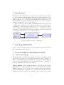
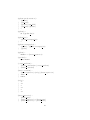
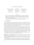
When executing the inverse method, Imitator takes as input a network
of PTAs with stopwatches and a reference valuation π0 ; it synthesizes a
constraint K on the parameters such that (1) π0 |= K and (2) for all parameter valuation π satisfying K, the trace set (i.e., the discrete behavior)
of A under π is the same as for A under π0 . This provides the system with
a criterion of robustness (see, e.g., [12]) around π0 .
PTA
Reference
valuation π0
Imitator
Constraint K
Figure 1: Functional view of Imitator
2
Installing IMITATOR
Sources, binaries for Linux platforms, and installation instructions are available on Imitator’s Web page [11].
3
3.1
General Structure and Implementation
Inputs and Outputs
The input syntax of Imitator to describe the network of PTAs modeling
the system is originally based on the HyTech syntax, with several improvements. Actually, all standard HyTech files describing only PTAs (and not
more general systems like linear hybrid automata[2]) can be analyzed directly by Imitator with very minor changes.
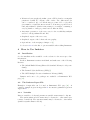
Inverse Method. When calling Imitator to apply the inverse method
algorithm, the tool takes as input two files, one describing the network of
PTAs modeling the system, and the other describing the reference valuation.
As depicted in Figure 2, it synthesizes a constraint on the parameters solving
the inverse problem, as well as optionally the corresponding trace set under
3
a graphical form. The description of all the parametric reachable states can
also be optionally output.
Constraint K0 on
the parameters
PTA A
Imitator
Reference
valuation π0
Trace set
(graphical form)
Figure 2: Imitator inputs and outputs in inverse method mode
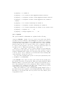
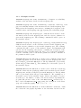
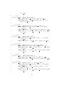
Behavioral Cartography Algorithm. When calling Imitator to apply
the behavioral cartography algorithm, the tool takes as an input two files,
one describing the network of PTAs modeling the system, and the other
describing the reference rectangle, i.e., the bounds to consider for each parameter. As depicted in Figure 3, it synthesizes a list of tiles, as well as
optionally the trace set corresponding to each tile under a graphical form.
The description of all the parametric reachable states for each tile may also
optionally be output.
PTA A
Reference
rectangle V0
List of tiles
Imitator
List of trace sets
(graphical form)
Figure 3: Imitator inputs and outputs in behavioral cartography mode
3.2
Features
Imitator (version 2.6.0) includes the following features:
• Analysis of a network of parametric timed automata augmented with
stopwatches and discrete rational-valued variables;
• Reachability analysis: given a PTA A, compute the set of all the
reachable states (as it is done in tools such as, e.g., HyTech and
PHAVer);
• Inverse method algorithm: given a PTA A and a reference valuation π0 , synthesize a constraint guaranteeing the same trace set as for
A[π0 ];
4
• Behavioral cartography algorithm: given a PTA A and a rectangular
parameter domain V0 , compute a list of tiles. Two different modes
can be considered: (1) cover all the integer points of V0 or, (2) call a
given number of times the inverse method on an integer point selected
randomly within V0 (which is interesting for rectangles containing a
very big number of integer points but few different tiles);
• Automatic generation of the trace sets, for the reachability analysis
and for both algorithms IM and BC ;
• Graphical output of the trace sets;
• Graphical output of the behavioral cartography;
• Optional use of the merging technique of [6].
See Section 4.3.4 for the list of options available when calling Imitator.
4
How to Use Imitator
4.1
Installation
See the installation files available on the website for the most up-to-date
information.
In short, Imitator is written in OCaml, and makes use of the following
libraries:
• The OCaml ExtLib library (Extended Standard Library for Objective
Caml)
• The Parma Polyhedra Library (PPL) [8]
• The GNU Multiple Precision Arithmetic Library (GMP)
Binaries and source code packages are available on Imitator’s Web
page [11].
4.2
The Imitator Input File
Examples of input files can be found on Imitator’s Web page [11]. A
complete example is given in Appendix A. A tentative grammar is given in
Appendix B.
4.2.1
Variables
Discrete variables, clocks and parameters variable names must be disjoint.
The synchronization label names may be identical to other names (automata or variables). The automata names may be identical to other names
(variables synchronization labels).
5
4.2.2
Parametric Timed Automata
See Appendix B.
4.2.3
Initial region and π0
See Appendix B.
4.3
Calling Imitator
Imitator can be used with three different modes:
1. Reachability analysis: given a PTA A, compute the whole set of reachable states from a given initial state.
2. Inverse Method: given a PTA A and a valuation π0 of the parameters, compute a constraint on the parameters guaranteeing the same
behavior as under π0 [7].
3. Behavioral Cartography Algorithm: given a PTA A and a rectangle V0
(bounded interval of values for each parameter), compute a cartography of the system [4].
We detail those three modes below.
4.3.1
Reachability Analysis
Given a PTA A, the reachability analysis computes the whole set of reachable states from a given initial state. The syntax in this case is the following
one:
IMITATOR <input file> -mode reachability [options]
Note that there is no need to provide a π0 or V0 file in this case (if one
is provided, it will be ignored).
4.3.2
Inverse Method
Given a PTA A and a valuation π0 of the parameters, the inverse method
compute a constraint K0 on the parameters guaranteeing that, for any π |=
K0 , the trace sets of A[π] and A[π0 ] are the same [7]. The syntax in this
case is the following one:
IMITATOR <input file> <pi0 file> [-mode inversemethod] [options]
Note that the -mode inversemethod option is not necessary, since the
default value for -mode is precisely inversemethod.
Note that, unlike the algorithm given in [7], at a given iteration, the
π0 -incompatible state is selected deterministically, for efficiency reasons.
However, the π0 -incompatible inequality within a π0 -incompatible state is
selected randomly, unless the -no-random option is activated.
6
In this case, Imitator outputs the resulting constraint K0 on the standard output.
4.3.3
Cartography
Given a PTA A and a rectangle V0 (bounded interval of values for each
parameter), the Behavioral Cartography Algorithm computes a cartography
of the system [4]. Two possible variants of the algorithm can be used:
1. The standard variant covers all the integer points within V0 . The
syntax in this case is the following one:
IMITATOR <input file> <V0 file> [-mode cover] [options]
2. The alternative variant calls the inverse method a certain number of
times on a random point V0 . The syntax in this case is the following
one:
IMITATOR <input file> <V0 file> [-mode randomX] [options]
where X represents the number of random points to consider. If a point
has already been generated before, the inverse method is not called.
If a point belongs to one of the tiles computed before, the inverse
method is not called neither. Therefore, in practice, the number of
tiles generated is smaller than X.
When in behavioral cartography mode, one can generate the cartography
in a graphical form (for 2 dimensions) using option -cart (see below). In
that case, an image will be output.
It is also possible to automatically color this cartography (in green and
red) according to a property to be verified. The property must be defined
at the end of the .imi model file, using the following syntax:
property := [PROP]
[PROP] must conform to one of the following patterns, where AUTOMATON
is an automaton name, LOCATION is a location name, a, a1, a2 are actions,
and the deadline d is a (possibly parametric) linear expression:
• property := unreachable loc[AUTOMATON] = LOCATION
• property := if a2 then a1 has happened before
• property := everytime a2 then a1 has happened before
• property := everytime a2 then a1 has happened once before
• property := if a1 then eventually a2
• property := everytime a1 then eventually a2
• property := everytime a1 then eventually a2 once before next
7
• property := a within d
• property := if a2 then a1 has happened within d before
• property := everytime a2 then a1 has happened within d before
• property := everytime a2 then a1 has happened once within d
before
• property := if a1 then eventually a2 within d
• property := everytime a1 then eventually a2 within d
• property := if a1 then eventually a2 within d once before next
• property := sequence a1, ..., an
• property := always sequence a1, ..., an
4.3.4
Options
The options available for Imitator are explained in the following.
-acyclic (default: false) Does not test if a new state was already
encountered. In a normal use, when Imitator encounters a new state, it
checks if it has been encountered before. This test may be time consuming
for systems with a high number of reachable states. For acyclic systems,
all traces pass only once by a given location. As a consquence, there are
no cycles, so there should be no need to check if a given state has been
encountered before. This is the main purpose of this option.
However, be aware that, even for acyclic systems, several (different)
traces can pass by the same state. In such a case, if the -acyclic option is
activated, Imitator will compute twice the states after the state common
to the two traces. As a consequence, it is all but sure that activating this
option will lead to an increase of speed.
Note also that activating this option for non-acyclic systems may lead
to an infinite loop in Imitator.
-cart (default: off) After execution of the behavioral cartography, plots
the generated zones as a PostScript file. This option takes an integer which
limits the number of generated plots, where each plot represents the projection of the parametric zones on two parameters. If the considered rectangle
v0 is spanned by two parameters only, then -cart 1 will plot the projection
of the generated zones on these two parameters.
This option makes use of the external utility graph, which is part of
the GNU plotting utils, available on most Linux platforms. The generated
files will be located in the same directory as the source files, unless option
-log-prefix is used.
8
-depth-limit <limit> (default: none) Limits the number of iterations
in the Post exploration, i.e., the depth of the traces. In the cartography
mode, this option gives a limit to each call to the inverse method.
-fancy (default: false) In the graphical output of the reachable states
(see option -with-dot), provide detailed information on the local states of
the composed automata.
-fromGrML (default: false) Does not use the standard input syntax
described here, but a GrML input syntax. This is used when interfacing
Imitator with the CosyVerif platform. Note that, in that case, not all
syntactic features of Imitator are supported.
-IMK (default: false) Uses a variant of the inverse method that returns a
constraint such that no π0 -compatible state is reached; it does not guarantee
however that any “good” state will be reached (see [7]).
-IMunion (default: false) Uses a variant of the inverse method that
returns the union of the constraints associated to the last state of each path
(see [7]).
-incl (default: false) Consider an inclusion of region instead of the
equality when performing the Post operation. In other terms, when encountering a new state, Imitator checks if the same state (same location and
same constraint) has been encountered before and, if yes, does not consider
this “new” state. However, when the -inclusion option is activated, it suffices that a previous state with the same location and a constraint greater
or equal to the constraint of the new state has been encountered to stop
the analysis. This option corresponds to the way that, e.g., HyTech works,
and suffices when one wants to check the non-reachability of a given bad
state.
-log-prefix (default: <input file>)
and graphical (.jpg) files.
Set the prefix for log (.states)
-merge (default: false) Use the merging technique of [6]. Note that, in
that case, not all the properties of the inverse method are preserved.
-mode (default: inversemethod)
The mode for Imitator.
9
Parametric reachability analysis
(see Section 4.3.1)
inversemethod Inverse method
(see Section 4.3.2)
cover
Behavioral Cartography Algorithm with full coverage
(see Section 4.3.3)
randomXX
Behavioral Cartography Algorithm with XX iterations
(see Section 4.3.3)
reachability
-no-random (default: false) No random selection of the π0 -incompatible
inequality (select the first found). By default, select an inequality in a
random manner.
-PTA2GrML (default: false)
mat, and exits.
Translates the input model to a GrML for-
-PTA2JPG (default: false) Translates the input model to a graphical,
human-readable form (in .jpg format), and exits.
-states-limit (default: none) Will try to stop after reaching this number of states. Warning: the program may have to first finish computing the
current iteration before stopping.
-statistics (default: false) Print info on number of calls to PPL, and
other statistics about memory and time. Warning: enabling this option may
slow down the analysis, and will certainly induce some extra computational
time at the end.
-step (default: 1)
Step for the behavioral cartography.
-sync-auto-detect (default: false) Imitator considers that all the
automata declaring a given synchronization label must be able to synchronize all together, so that the synchronization can happen. By default, Imitator considers that the synchronization labels declared in an automaton
are those declared in the synclabs section. Therefore, if a synchronization
label is declared but never used in (at least) one automaton, this label will
never be synchronized in the execution1 .
The option -sync-auto-detect allows to detect automatically the synchronization labels in each automaton: the labels declared in the synclabs
section are ignored, and the Imitator considers that only the labels really
used in an automaton are those considered to be declared.
1
In such a case, the synchronization label is actually completely removed before the
execution, in order to optimize the execution, and the user is warned of this removal.
10
-time-limit <limit> (default: none) Try to limit the execution time
(the value <limit> is given in seconds). Note that, in the current version of
Imitator, the test of time limit is performed at the end of an iteration only
(i.e., at the end of a given Post iteration). In the cartography mode, this
option represents a global time limit, not a limit for each call to the inverse
method.
-timed (default: false)
program.
Add a timing information to each output of the
-verbose (default: standard) Give some debugging information, that
may also be useful to have more details on the way Imitator works. The
admissible values for -verbose are given below:
nodebug Give only the resulting constraint
standard Give little information (number of steps, computation time)
low
Give little additional information
medium
Give quite a lot of information
high
Give much information
total
Give really too much information
-with-dot (default: false) Graphical output using dot. In this case,
Imitator outputs a file <input file>.jpg, which is a graphical output in
the jpg format, generated using dot, corresponding to the trace set.
Note that the location and the name of those two files can be changed
using the -log-prefix option.
-with-graphics-source (default: false)
graphical outputs.
Keep file(s) generated for the
-with-log (default: false) Generation of the files describing the reachable states. In this case, Imitator outputs a file <input file>.states
containing the set of all the reachable states, with their names and the associated constraint on the clocks and parameters. If one wants to generate
also the constraint on the parameters only, use the -with-parametric-log
option. This file also contains the source for the generation of the graphical
file, using the dot syntax.
-with-parametric-log (default: false) For any constraint on the
clocks and the parameters in the description of the states in the log files,
add the constraint on the parameters only (i.e., eliminate clock variables).
11
4.3.5
Examples of Calls
IMITATOR flipflop.imi -mode reachability Computes a reachability
analysis on the automata described in file flipflop.imi.
IMITATOR flipflop.imi -mode reachability -with-dot -with-log Computes a reachability analysis on the automata described in file flipflop.imi.
Will generate files flipflop.imi.states, containing the description of the
reachable states, and flipflop.imi.jpg depicting the reachability graph.
IMITATOR flipflop.imi flipflop.pi0 Calls the inverse method on the
automata described in file flipflop.imi, and the reference valuation π0
given in file flipflop.pi0. The resulting constraint K0 will be given on
the standard output.
IMITATOR flipflop.imi flipflop.pi0 -with-log -with-parametric-log
Calls the inverse method on the automata described in file flipflop.imi,
and the reference valuation π0 given in file flipflop.pi0. The resulting
constraint K0 will be given on the standard output. and Imitator will
generate the file flipflop.imi.states, containing the description of the
(parametric) states reachable under K0 . Moveover, for any state in this file,
both the constraint on the clocks and the parameters, and the constraint on
the parameters will be given.
IMITATOR SRlatch.imi SRlatch.v0 -mode cover Calls the behavioral cartography algorithm on the automata described in file flipflop.imi, and
the rectangle V0 given in file SRlatch.v0. The algorithm will cover (at least)
all the integer points within V0 . The resulting set of tiles will be given on
the standard output.
IMITATOR SRlatch.imi SRlatch.v0 -mode cover -with-dot -with-log
Calls the behavioral cartography algorithm on the automata described in file
flipflop.imi, and the rectangle V0 given in file SRlatch.v0. The algorithm
will cover (at least) all the integer points within V0 . The resulting set of
tiles will be given on the standard output. Given n the number of generated tiles (i.e., the number of calls to the inverse method algorithm), the
program will generate n files of the form SRlatch.imi i.states (resp. n
files of the form SRlatch.imi i.jpg) giving the description of the states
(resp. the reachability graph) of tile i, for i = 1, . . . , n.
IMITATOR SRlatch.imi SRlatch.v0 -mode random100 -with-dot Calls
the behavioral cartography algorithm on the automata described in file
12
R
Q
S

Q
S
R
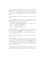
t↓
Figure 4: SR latch (left) and environment (right)
flipflop.imi, and the rectangle V0 given in file SRlatch.v0. The program will call the inverse method on 100 points randomly selected within
V0 . Since some points may be generated several times, or some points may
belong to previously generated tiles (see Section 4.3.3), the number n of
tiles generated will be such that n ≤ 100. The program will generate n files
of the form SRlatch.imi i.jpg giving the reachability graph of tile i, for
i = 1, . . . , n.
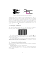
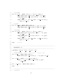
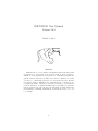
5
Example: SR-latch
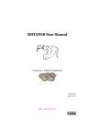
We consider a SR-latch described in, e.g., [10], and depicted on Figure 4
left. The possible configurations of the latch are the following ones:
S R
Q
Q
0 0 latch latch
0 1
0
1
1 0
1
0
1 1
0
0
We consider an initial configuration with R = S = 1 and Q = Q = 0.
As depicted in Figure 4, the signal S first goes down. Then, the signal R
goes down after a time t↓ .
We consider that the gate Nor 1 (resp. Nor 2 ) has a punctual parametric
delay δ1 (resp. δ2 ). Moreover, the parameter t↓ corresponds to the time
duration between the fall of S and the fall of R.
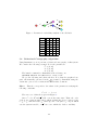
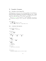
5.1
Parametric Reachability Analysis
We first perform a reachability analysis. The launch command for Imitator
is the following one:
IMITATOR SRlatch.imi -mode reachability
Considering this environment, the trace set of this system is given in
Figure 5, where the states qi , i = 0, . . . , 6 correspond to the following values
for each signal:
13
Q
q0
S↓
q3
↑
R↓
q6
↑
q1
R↓
q2
Q
Q↑
q4
q5
Figure 5: Parametric reachability analysis of the SR latch
State
q0
q1
q2
q3
q4
q5
q6
5.2
S
1
0
0
0
0
0
0
R
1
1
0
1
0
0
0
Q
0
0
0
0
0
1
0
Q
0
0
0
1
1
0
1
Behavioral Cartography Algorithm
Using Imitator, we now perform a behavioral cartography of this system.
We consider the following rectangle V0 for the parameters:
t↓ ∈ [0, 10]
δ1 ∈ [0, 10]
δ2 ∈ [0, 10]
The launch command for Imitator is the following one:
IMITATOR SRlatch.imi SRlatch.v0 -mode cover
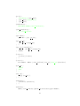
We get the following six behavioral tiles. Note that the graphical outputs, automatically generated in the jpg format by Imitator using the
-with-dot option, were rewritten in LATEX in this document.
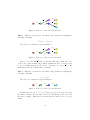
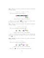
Tile 1. This tile corresponds to the values of the parameters verifying the
following constraint:
t↓ = δ2 ∧ δ1 = 0
The trace set of this tile is given in Figure 6.
↑
Since t↓ = δ2 , R↓ and Q will occur at the same time. Thus, the order
of those two events is unspecified, which explains the choice between going
to q2 or q3 . When in state q2 , either Q↑ can occur (since δ1 = 0), in which
↑
case the system is stable, or Q can occur, which also leads to stability.
14
Q
q0
↑
q3
R↓
q6
↑
S↓
q1
R↓
q2
Q
Q↑
q4
q5
Figure 6: Trace set of tile 1 for the SR latch
Tile 2. This tile corresponds to the values of the parameters verifying the
following constraint:
t↓ = δ2 ∧ δ1 > 0
The trace set of this tile is given in Figure 7.
Q
q0
↑
q3
R↓
q6
↑
S↓
q1
R↓
q2
Q
q4
Figure 7: Trace set of tile 2 for the SR latch
↑
Since t↓ = δ2 , R↓ and Q will occur at the same time. Thus, the order
of those two events is unspecified, which explains the choice between going
↑
to q2 or q3 . When in state q2 , Q↑ can not occur (since δ1 > 0), so Q occurs
immediately after R↓ , which leads to stability.
Tile 3. This tile corresponds to the values of the parameters verifying the
following constraint:
δ2 > t↓ + δ1
The trace set of this tile is given in Figure 8.
q0
S↓
q1
R↓
q2
Q↑
q5
Figure 8: Trace set of tile 3 for the SR latch
In this case, since δ2 > t↓ + δ1 , S ↓ will occur before the gate Nor 2 has
the time to change. For the same reason, Q↑ will change before Nor 1 has
the time to change. With Q = 1, the system is now stable: Nor 1 does not
change.
15
Tile 4. This tile corresponds to the values of the parameters verifying the
following constraint:
t↓ + δ1 = δ2 ∧ δ2 ≥ δ1 ∧ δ1 > 0
The trace set of this tile is given in Figure 9.
q0
S↓
q1
R↓
q2
Q↑
Q
↑
q5
q4
Figure 9: Trace set of tile 4 for the SR latch
↑
Since t↓ + δ1 = δ2 , both Q↑ or Q can occur. Once one of them occured,
the system gets stable, and no other change occurs.
Tile 5. This tile corresponds to the values of the parameters verifying the
following constraint:
δ2 > t↓ ∧ t↓ + δ1 > δ2
The trace set of this tile is given in Figure 10.
q0
S↓
q1
R↓
↑
q2
Q
q4
Figure 10: Trace set of tile 5 for the SR latch
Since δ2 > t↓ , the gate Nor 2 can not change before R↓ occurs. However,
since t↓ + δ1 > δ2 , the gate Nor 2 changes before Q↑ can occur, thus leading
↑
to event Q .
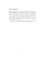
Tile 6. This tile corresponds to the values of the parameters verifying the
following constraint:
t↓ > δ2
The trace set of this tile is given in Figure 11.
q0
S↓
↑
q1
Q
q3
R↓
q6
Figure 11: Trace set of tile 6 for the SR latch
↑
Since t↓ > δ2 , Q occurs before S ↓ . The system is then stable.
16
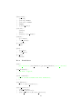
Cartography. We give in Figure 12 the cartography of the SR latch example. For the sake of simplicity of representation, we consider only parameters
δ1 and δ2 . Therefore, we set t↓ = 1.
δ2
4
3
5
1
2
6
δ1
Figure 12: Behavioral cartography of the SR latch according to δ1 and δ2
Note that tile 1 corresponds to a point, and tiles 2 and 4 correspond to
lines.
The rectangle V0 has been represented with dashed lines. Note that all
tiles (except tile 1) are unbounded, so that they cover, not only V0 , but all
the positive real-valued plan.
The source code of this example is available in Appendix A.
17
Acknowledgments
´
Etienne
Andr´e initiated the development of Imitator, and keeps developing it. Emmanuelle Encrenaz and Laurent Fribourg have been great contributors of Imitator, on a theoretical point of view, and to find applications both from the literature and real case studies. Abdelrezzak Bara
provided several examples from the hardware literature. Jeremy Sproston
provided examples from the probabilistic community. Ulrich K¨
uhne made
several important improvements to Imitator, and linked the tool to PPL.
Daphne Dussaud implemented the graphical output of the behavioral cartography. Romain Soulat implemented powerful algorithmic optimizations,
and brought many case studies.
Imitator’s logo comes from KaterBegemot’s Typing monkey.svg (Licence: Creative Commons Attribution-Share Alike 3.0 Unported).
18
References
[1] Y. Adbedda¨ım and O. Maler. Preemptive job-shop scheduling using
stopwatch automata. In J.-P. Katoen and P. Stevens, editors, Proceedings of the 8th International Conference on Tools and Algorithms
for Construction and Analysis of Systems (TACAS’02), volume 2280
of Lecture Notes in Computer Science, pages 113–126. Springer-Verlag,
Apr. 2002. 3
[2] R. Alur, C. Courcoubetis, T. A. Henzinger, and P.-H. Ho. Hybrid
automata: An algorithmic approach to the specification and verification
of hybrid systems. In R. L. Grossman, A. Nerode, A. P. Ravn, and
H. Rischel, editors, Hybrid Systems 1992, volume 736 of Lecture Notes
in Computer Science, pages 209–229. Springer, 1993. 3
[3] R. Alur, T. A. Henzinger, and M. Y. Vardi. Parametric real-time reasoning. In Proceedings of the twenty-fifth annual ACM symposium on
Theory of computing, STOC’93, pages 592–601, New York, NY, USA,
1993. ACM. 3
´ Andr´e and L. Fribourg. Behavioral cartography of timed automata.
[4] E.
In A. Kuˇcera and I. Potapov, editors, Proceedings of the 4th Workshop
on Reachability Problems in Computational Models (RP’10), volume
6227 of Lecture Notes in Computer Science, pages 76–90, Brno, Czech
Republic, Aug. 2010. Springer. 6, 7
´ Andr´e, L. Fribourg, U. K¨
[5] E.
uhne, and R. Soulat. IMITATOR 2.5:
A tool for analyzing robustness in scheduling problems. In D. Giannakopoulou and D. M´ery, editors, Proceedings of the 18th International
Symposium on Formal Methods (FM’12), volume 7436 of Lecture Notes
in Computer Science, pages 33–36, Paris, France, Aug. 2012. Springer.
1, 3
´ Andr´e, L. Fribourg, and R. Soulat. Enhancing the inverse method
[6] E.
with state merging. In A. Goodloe and S. Person, editors, Proceedings of
the 4th NASA Formal Methods Symposium (NFM’12), volume 7226 of
Lecture Notes in Computer Science, pages 100–105, Norfolk, Virginia,
USA, Apr. 2012. Springer. 5, 9
´ Andr´e and R. Soulat. The Inverse Method. ISTE Ltd and John
[7] E.
Wiley & Sons Inc., 2013. 176 pages. 3, 6, 9
[8] R. Bagnara, P. M. Hill, and E. Zaffanella. The Parma Polyhedra Library: Toward a complete set of numerical abstractions for the analysis
and verification of hardware and software systems. Science of Computer
Programming, 72(1–2):3–21, 2008. 5
19
[9] E. M. Clarke, O. Grumberg, S. Jha, Y. Lu, and H. Veith.
Counterexample-guided abstraction refinement. In CAV’00, pages 154–
169. Springer-Verlag, 2000. 3
[10] D. Harris and S. Harris. Digital Design and Computer Architecture.
Morgan Kaufmann Publishers Inc., San Francisco, CA, USA, 2007. 13
[11] IMITATOR Team. IMITATOR Web page, 2013. 3, 5
[12] N. Markey. Robustness in real-time systems. In Proceedings of the
6th IEEE International Symposium on Industrial Embedded Systems
(SIES’11), pages 28–34, V¨aster˚
as, Sweden, June 2011. IEEE Computer
Society Press. 3
20
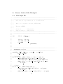
A
A.1
1
2
3
4
5
6
7
8
9
10
11
12
Source Code of the Example
Main Input File
−−∗∗∗∗∗∗∗∗∗∗∗∗∗∗∗∗∗∗∗∗∗∗∗∗∗∗∗∗∗∗∗∗∗∗∗∗∗∗∗∗∗∗∗∗∗∗∗∗∗∗∗∗∗∗∗∗∗∗∗∗ − −
−−∗∗∗∗∗∗∗∗∗∗∗∗∗∗∗∗∗∗∗∗∗∗∗∗∗∗∗∗∗∗∗∗∗∗∗∗∗∗∗∗∗∗∗∗∗∗∗∗∗∗∗∗∗∗∗∗∗∗∗∗ − −
−−
Laboratoire S p e c i f i c a t i o n et V e r i f i c a t i o n
−−
−−
Race on a d i g i t a l c i r c u i t (SR Latch )
−−
−−
E t i e n n e ANDRE
−−
−−
Created :
2010/03/19
−−
Last m o d i f i e d : 2013/03/07
−−∗∗∗∗∗∗∗∗∗∗∗∗∗∗∗∗∗∗∗∗∗∗∗∗∗∗∗∗∗∗∗∗∗∗∗∗∗∗∗∗∗∗∗∗∗∗∗∗∗∗∗∗∗∗∗∗∗∗∗∗ − −
−−∗∗∗∗∗∗∗∗∗∗∗∗∗∗∗∗∗∗∗∗∗∗∗∗∗∗∗∗∗∗∗∗∗∗∗∗∗∗∗∗∗∗∗∗∗∗∗∗∗∗∗∗∗∗∗∗∗∗∗∗ − −
13
14
15
var
ckNor1 , ckNor2 , s
: clock ;
16
17
18
19
20
dNor1 l , dNor1 u ,
dNor2 l , dNor2 u ,
t down
: parameter ;
21
22
23
24
25
26
27
−−∗∗∗∗∗∗∗∗∗∗∗∗∗∗∗∗∗∗∗∗∗∗∗∗∗∗∗∗∗∗∗∗∗∗∗∗∗∗∗∗∗∗∗∗∗∗∗∗∗∗∗∗∗∗∗∗∗∗∗∗ − −
automaton norGate1
−−∗∗∗∗∗∗∗∗∗∗∗∗∗∗∗∗∗∗∗∗∗∗∗∗∗∗∗∗∗∗∗∗∗∗∗∗∗∗∗∗∗∗∗∗∗∗∗∗∗∗∗∗∗∗∗∗∗∗∗∗ − −
synclabs : R Up , R Down , overQ Up , overQ Down ,
Q Up , Q Down ;
28
29
30
31
32
33
−− UNSTABLE
loc Nor1 000 : while ckNor1 <= dNor1 u wait {}
when True sync R Up do {} goto Nor1 100 ;
when True sync overQ Up do {} goto Nor1 010 ;
when ckNor1 >= d N o r 1 l sync Q Up do {} goto
Nor1 001 ;
34
35
36
37
38
−− STABLE
loc Nor1 001 : while True wait {}
when True sync R Up do { ckNor1 ’ = 0} goto
Nor1 101 ;
when True sync overQ Up do { ckNor1 ’ = 0} goto
21
Nor1 011 ;
39
40
41
42
43
−− STABLE
loc Nor1 010 : while True wait {}
when True sync R Up do {} goto Nor1 110 ;
when True sync overQ Down do { ckNor1 ’ = 0}
goto Nor1 000 ;
44
45
46
47
48
49
−− UNSTABLE
loc Nor1 011 : while ckNor1 <= dNor1 u wait {}
when True sync R Up do { ckNor1 ’ = 0} goto
Nor1 111 ;
when True sync overQ Down do {} goto Nor1 001 ;
when ckNor1 >= d N o r 1 l sync Q Down do {} goto
Nor1 010 ;
50
51
52
53
54
−− STABLE
loc Nor1 100 : while True wait {}
when True sync R Down do { ckNor1 ’ = 0} goto
Nor1 000 ;
when True sync overQ Up do {} goto Nor1 110 ;
55
56
57
58
59
60
−− UNSTABLE
loc Nor1 101 : while ckNor1 <= dNor1 u wait {}
when True sync R Down do {} goto Nor1 001 ;
when True sync overQ Up do { ckNor1 ’ = 0} goto
Nor1 111 ;
when ckNor1 >= d N o r 1 l sync Q Down do {} goto
Nor1 100 ;
61
62
63
64
65
−− STABLE
loc Nor1 110 : while True wait {}
when True sync R Down do {} goto Nor1 010 ;
when True sync overQ Down do {} goto Nor1 100 ;
66
67
68
69
70
71
−− UNSTABLE
loc Nor1 111 : while ckNor1 <= dNor1 u wait {}
when True sync R Down do { ckNor1 ’ = 0} goto
Nor1 011 ;
when True sync overQ Down do { ckNor1 ’ = 0}
goto Nor1 101 ;
when ckNor1 >= d N o r 1 l sync Q Down do {} goto
Nor1 110 ;
72
22
73
end −− norGate1
74
75
76
77
78
79
80
81
−−∗∗∗∗∗∗∗∗∗∗∗∗∗∗∗∗∗∗∗∗∗∗∗∗∗∗∗∗∗∗∗∗∗∗∗∗∗∗∗∗∗∗∗∗∗∗∗∗∗∗∗∗∗∗∗∗∗∗∗∗ − −
automaton norGate2
−−∗∗∗∗∗∗∗∗∗∗∗∗∗∗∗∗∗∗∗∗∗∗∗∗∗∗∗∗∗∗∗∗∗∗∗∗∗∗∗∗∗∗∗∗∗∗∗∗∗∗∗∗∗∗∗∗∗∗∗∗ − −
synclabs : Q Up , Q Down , S Up , S Down ,
overQ Up , overQ Down ;
−− i n i t i a l l y Nor2 110 ;
82
83
84
85
86
87
−− UNSTABLE
loc Nor2 000 : while ckNor2 <= dNor2 u wait {}
when True sync Q Up do {} goto Nor2 100 ;
when True sync S Up do {} goto Nor2 010 ;
when ckNor2 >= d N o r 2 l sync overQ Up do {}
goto Nor2 001 ;
88
89
90
91
92
−− STABLE
loc Nor2 001 : while True wait {}
when True sync Q Up do { ckNor2 ’ = 0} goto
Nor2 101 ;
when True sync S Up do { ckNor2 ’ = 0} goto
Nor2 011 ;
93
94
95
96
97
−− STABLE
loc Nor2 010 : while True wait {}
when True sync Q Up do {} goto Nor2 110 ;
when True sync S Down do { ckNor2 ’ = 0} goto
Nor2 000 ;
98
99
100
101
102
103
−− UNSTABLE
loc Nor2 011 : while ckNor2 <= dNor2 u wait {}
when True sync Q Up do { ckNor2 ’ = 0} goto
Nor2 111 ;
when True sync S Down do {} goto Nor2 001 ;
when ckNor2 >= d N o r 2 l sync overQ Down do {}
goto Nor2 010 ;
104
105
106
107
108
−− STABLE
loc Nor2 100 : while True wait {}
when True sync Q Down do { ckNor2 ’ = 0} goto
Nor2 000 ;
when True sync S Up do {} goto Nor2 110 ;
109
23
110
111
112
113
114
−− UNSTABLE
loc Nor2 101 : while ckNor2 <= dNor2 u wait {}
when True sync Q Down do {} goto Nor2 001 ;
when True sync S Up do { ckNor2 ’ = 0} goto
Nor2 111 ;
when ckNor2 >= d N o r 2 l sync overQ Down do {}
goto Nor2 100 ;
115
116
117
118
119
−− STABLE
loc Nor2 110 : while True wait {}
when True sync Q Down do {} goto Nor2 010 ;
when True sync S Down do {} goto Nor2 100 ;
120
121
122
123
124
125
−− UNSTABLE
loc Nor2 111 : while ckNor2 <= dNor2 u wait {}
when True sync Q Down do { ckNor2 ’ = 0} goto
Nor2 011 ;
when True sync S Down do { ckNor2 ’ = 0} goto
Nor2 101 ;
when ckNor2 >= d N o r 2 l sync overQ Down do {}
goto Nor2 110 ;
126
127
end −− norGate2
128
129
130
131
132
133
−−∗∗∗∗∗∗∗∗∗∗∗∗∗∗∗∗∗∗∗∗∗∗∗∗∗∗∗∗∗∗∗∗∗∗∗∗∗∗∗∗∗∗∗∗∗∗∗∗∗∗∗∗∗∗∗∗∗∗∗∗ − −
automaton env
−−∗∗∗∗∗∗∗∗∗∗∗∗∗∗∗∗∗∗∗∗∗∗∗∗∗∗∗∗∗∗∗∗∗∗∗∗∗∗∗∗∗∗∗∗∗∗∗∗∗∗∗∗∗∗∗∗∗∗∗∗ − −
synclabs : R Down , R Up , S Down , S Up ;
134
135
136
137
−− ENVIRONMENT : f i r s t S then R a t c o n s t a n t time
loc e n v 1 1 : while True wait {}
when True sync S Down do { s ’ = 0} goto e n v 1 0 ;
138
139
140
loc e n v 1 0 : while s <= t down wait {}
when s = t down sync R Down do {} goto
env final ;
141
142
loc e n v f i n a l : while True wait {}
143
144
end −− env
145
146
147
−−∗∗∗∗∗∗∗∗∗∗∗∗∗∗∗∗∗∗∗∗∗∗∗∗∗∗∗∗∗∗∗∗∗∗∗∗∗∗∗∗∗∗∗∗∗∗∗∗∗∗∗∗∗∗∗∗∗∗∗∗ − −
−− ANALYSIS
24
148
−−∗∗∗∗∗∗∗∗∗∗∗∗∗∗∗∗∗∗∗∗∗∗∗∗∗∗∗∗∗∗∗∗∗∗∗∗∗∗∗∗∗∗∗∗∗∗∗∗∗∗∗∗∗∗∗∗∗∗∗∗ − −
149
150
151
152
153
154
155
156
157
i n i t := True
−−−−−−−−−−−−−−−−−−−−−−−−−−−−−−−−−−−−−−−−−−−−−−−−−−−−−−−−−−−−
−− INITIAL LOCATIONS
−−−−−−−−−−−−−−−−−−−−−−−−−−−−−−−−−−−−−−−−−−−−−−−−−−−−−−−−−−−−
−− S and R down
& loc [ norGate1 ] = Nor1 100
& loc [ norGate2 ] = Nor2 010
& loc [ env ]
= env 11
158
−−−−−−−−−−−−−−−−−−−−−−−−−−−−−−−−−−−−−−−−−−−−−−−−−−−−−−−−−−−−
−− INITIAL CONSTRAINTS
−−−−−−−−−−−−−−−−−−−−−−−−−−−−−−−−−−−−−−−−−−−−−−−−−−−−−−−−−−−−
& ckNor1
= 0
& ckNor2
= 0
& s
= 0
159
160
161
162
163
164
165
& d N o r 1 l >= 0
& d N o r 2 l >= 0
166
167
168
& d N o r 1 l <= dNor1 u
& d N o r 2 l <= dNor2 u
169
170
171
;
A.2
1
2
3
4
5
6
7
8
V0 File
−−−−−−−−−−−−−−−−−−−−−−−−−−−−−−−−−−−−−−−−−−−−−−−−−−−−−−−−−−−−
−− V0
−−−−−−−−−−−−−−−−−−−−−−−−−−−−−−−−−−−−−−−−−−−−−−−−−−−−−−−−−−−−
& dNor1 l
= 3
& dNor1 u
= 3 . . 20
& dNor2 l
= 5
& dNor2 u
= 5 . . 20
& t down
= 10
25
B
Complete Grammar
B.1
Grammar of the Input File
Imitator input is described by the following grammar. Non-terminals appear within angled parentheses. A non-terminal followed by two colons is
defined by the list of immediately following non-blank lines, each of which
represents a legal expansion. Input characters of terminals appear in typewritter font. The meta symbol denotes the empty string.
The text in green is not taken into account by Imitator, but is allowed
(or sometimes necessary) in order to allow the compatibility with HyTech
files.
himitator inputi ::
hautomata descriptionsi hiniti
We define each of those two components below.
B.1.1
Automata Descriptions
hautomata descriptionsi ::
hdeclarationsi hautomatai
hdeclarationsi ::
var hvar listsi
hvar listsi ::
hvar listi : hvar typei ; hvar listsi
| hvar listi ::
<name>
| <name> , hvar listi
hvar typei ::
clock
| discrete
| parameter
hautomatai ::
hautomatoni hautomatai
| hautomatoni ::
automaton <name> hprologi hlocationsi end
26
hprologi ::
hinitializationi hsync labelsi
| hsync labelsi hinitializationi
| hsync labelsi
hinitializationi ::
initially <name> hstate initializationi ;
hstate initializationi ::
& hconvex predicatei
| hsync labelsi ::
synclabs : hsync var listi ;
hsync var listi ::
hsync var nonempty listi
| hsync var nonempty listi ::
<name> , hsync var nonempty listi
| <name>
hlocationsi ::
hlocationi hlocationsi
| hlocationsi ::
loc <name> : while hconvex predicatei hstop opti hwait opti htransitionsi
hwait opti ::
wait()
| wait
| hstop opti ::
stop{ hvar listi }
| htransitionsi ::
htransitioni htransitionsi
| htransitioni ::
when hconvex predicatei hupdate synchronizationi goto <name> ;
27
hupdate synchronizationi ::
hupdatesi
| hsyn label i
| hupdatesi hsyn label i
| hsyn label i hupdatesi
| hupdatesi ::
do ( hupdate listi )
hupdate listi ::
hupdate nonempty listi
| hupdate nonempty listi ::
hupdatei , hupdate nonempty listi
| hupdatei
hupdatei ::
<name> ’ = hlinear expressioni
hsyn label i ::
sync <name>
hconvex predicatei ::
hlinear constrainti & hconvex predicatei
| hlinear constrainti
hlinear constrainti ::
hlinear expressioni hrelopi hlinear expressioni
| True
| False
hrelopi ::
<
| <=
| =
| >=
| >
| <>
hlinear expressioni ::
hlinear termi
| hlinear expressioni + hlinear termi
| hlinear expressioni - hlinear termi
28
hlinear termi ::
hrational i
| hrational i <name>
| hrational i * <name>
| <name>
| ( hlinear termi )
hrational i ::
hinteger i
hfloati
| hinteger i / hpos integer i
hinteger i ::
hpos integer i
| - hpos integer i
hpos integer i ::
<int>
hfloati ::
hpos floati
| - hpos floati
hpos floati ::
<float>
B.1.2
Initial State
hiniti ::
hinit declarationi hinit definitioni hproperty definitioni hreach command i
hinit declarationi ::
var init : region ;
| hreach command i ::
print ( reach forward from init endreach ) ;
| hinit definitioni ::
init := hregion expressioni ;
hregion expressioni ::
hstate predicatei
| ( hregion expressioni )
| hregion expressioni & hregion expressioni
29
hstate predicatei ::
loc [ <name> ] = <name>
| hlinear constrainti
hproperty definitioni ::
property := hpatterni ;
| hpatterni ::
unreachable hloc predicatei
| if <name> then <name> has happened before
| everytime <name> then <name> has happened before
| everytime <name> then <name> has happened once before
| if <name> then eventually <name>
| everytime <name> then eventually <name>
| everytime <name> then eventually <name> once before next
| <name> within hlinear expressioni
| if <name> then <name> happened within hlinear expressioni before
| everytime <name> then <name> happened within hlinear expressioni before
| everytime <name> then <name> happened once within hlinear expressioni before
| if <name> then eventually <name> within hlinear expressioni
| everytime <name> then eventually <name> within hlinear expressioni
| everytime <name> then eventually <name> within hlinear expressioni once before next
| sequence hvar listi
| sequence always hvar listi
hloc expressioni ::
hloc predicatei
| hloc predicatei & hloc expressioni
| hloc predicatei hloc expressioni
hloc predicatei ::
loc[ <name> ] = <name>
B.2
Reserved Words
The following words are keywords and cannot be used as names for automata, variables, synchronization labels or locations.
always, and, automaton, bad, before, carto, clock, discrete, do, end,
eventually, everytime, False, goto, happened, has, if, init, initially,
loc, locations, next, not, once, or, parameter, property, region, sequence,
stop, sync, synclabs, then, True, unreachable, var, wait, when, while,
within
30