Download Sensor Based Robot Control - DTU Electronic Theses and

Mikkel Ørum Wahlgreen s042157
Daniel Esteban Morales Bondy s051976
Sensor Based Robot Control
Bachelor thesis, November 2009
Abstract
This projects describes the efforts to create a solution to an industrial problem. A 6-joint, 6
degree of freedom robot arm was used to simulate the deburring of a metal plate. A 6-axis
force/torque sensor was placed at the tool tip, allowing force regulation in the process. A
mock-up of a deburring machine was built, and the robot managed to simulate the deburr
proces of four sides of a metal plate.
Abstract
Gennem dette projekt er bestræbelserne på at finde en løsning på en industriel problematik beskrevet. En 6-leds, 6 friheds grader robot arm var brugt til at simulere afgratningsprocessen af en metalplade. En 6-akselede kræft/moment sensor blev placeret for
enden af robotten, hvilket gav en tilbagekobling i processen. En træmodel af en afgratningsmaskine blev bygget og robotten var i stand til at simulere afgratningsprocessen på
fire kanter af metalpladen.
Foreword
We would like to thank the people at AUT DTU, especially the following people:
Nils Axel Andersen and Ole Ravn, our supervisors.
Henrik Poulsen, who built our mock-up of the deburr tool.
Also a thanks to Universal Robots for letting us borrow their robot, especially Esben
H. Østergaard, who helped with troubleshooting.
Last but not least a thanks to Rene Bondy, who showed us how deburring is done in
the industry, and providing positive feedback.
1
Contents
1 Introduction
6
2 Problem Statement
7
3 Problem Delimitation
8
4 Theory
4.1 Deburring . . . . . . . . . . . . . . .
4.1.1 Robot deburring . . . . . . .
4.1.2 Tool Considerations . . . . . .
4.1.3 Safety Considerations . . . . .
4.2 Kinematics and Mathematics . . . .
4.2.1 Denavit-Hartenberg Notation
4.2.2 Path generation . . . . . . . .
4.3 Python programming . . . . . . . . .
4.4 Linear control . . . . . . . . . . . . .
.
.
.
.
.
.
.
.
.
9
9
9
13
15
15
16
18
19
19
5 Equipment description
5.1 Force sensor . . . . . . . . . . . . . . . . . . . . . . . . . . . . . . . . . . .
5.2 The UR-6-85-5-A robot . . . . . . . . . . . . . . . . . . . . . . . . . . . . .
21
21
22
6 Implementation
6.1 Analysis of Solutions . . . . . . . . . . . .
6.2 Method Implementation . . . . . . . . . .
6.2.1 Deburr Process . . . . . . . . . . .
6.2.2 Linear control design and kinematic
.
.
.
.
25
25
25
28
29
7 Programming the robot
7.1 Functions and their uses . . . . . . . . . . . . . . . . . . . . . . . . . . . .
7.2 User manual for the program . . . . . . . . . . . . . . . . . . . . . . . . . .
32
32
33
8 Calibration and Test
8.1 Test of communication speed . . . . . . . . . . . . . . . . . . . . . . . . . .
8.2 Force feedback during deburr . . . . . . . . . . . . . . . . . . . . . . . . .
35
35
36
2
.
.
.
.
.
.
.
.
.
.
.
.
.
.
.
.
.
.
.
.
.
.
.
.
.
.
.
.
.
.
.
.
.
.
.
.
.
.
.
.
.
.
.
.
.
.
.
.
.
.
.
.
.
.
.
.
.
.
.
.
.
.
.
. . . .
. . . .
. . . .
values
.
.
.
.
.
.
.
.
.
.
.
.
.
.
.
.
.
.
.
.
.
.
.
.
.
.
.
.
.
.
.
.
.
.
.
.
.
.
.
.
.
.
.
.
.
.
.
.
.
.
.
.
.
.
.
.
.
.
.
.
.
.
.
.
.
.
.
.
.
.
.
.
.
.
.
.
.
.
.
.
.
.
.
.
.
.
.
.
.
.
.
.
.
.
.
.
.
.
.
.
.
.
.
.
.
.
.
.
.
.
.
.
.
.
.
.
.
.
.
.
.
.
.
.
.
.
.
.
.
.
.
.
.
.
.
.
.
.
.
.
.
.
.
.
.
.
.
.
.
.
.
.
.
.
.
.
.
.
.
.
.
.
.
.
.
.
.
.
.
CONTENTS
8.3
3
Noise on the force sensor . . . . . . . . . . . . . . . . . . . . . . . . . . . .
37
9 Errors in the robot
40
10 Conclusion
42
11 Future Work
43
References
45
A Force error on the axes
46
B CD List of Contents
56
C Drawing of force sensor
58
D Drawing of the victim element
60
E Drawing of the deburr tool model
62
F Source code
F.0.1 maindeburr.py . . . . . . .
F.0.2 connectionregulatortest.py
F.0.3 force.py . . . . . . . . . .
F.0.4 force_test.py . . . . . . .
65
65
76
92
95
.
.
.
.
.
.
.
.
.
.
.
.
.
.
.
.
.
.
.
.
.
.
.
.
.
.
.
.
.
.
.
.
.
.
.
.
.
.
.
.
.
.
.
.
.
.
.
.
.
.
.
.
.
.
.
.
.
.
.
.
.
.
.
.
.
.
.
.
.
.
.
.
.
.
.
.
.
.
.
.
.
.
.
.
.
.
.
.
.
.
.
.
Reading guide
All of the concepts and theories needed to understand how the solution presented in this
report works can be found in the theory section. It is not required to have a deep understandig of the presented concepts, although if the reader wishes to have more knowledge
related to these topics, it is recommended to read the references, especially [OI09].
This report is written by two Bachelor of Science students at DTU and is meant to document a test-bench solution for a given problem. This problem is to simulate a deburr
process of a plate of aluminium with the UR-6-85-5-A robot. To be able to read and understand this report, the reader should have some basic knowledge about topics concerning
control of robots, math, and programming languages. The following topics are essential
for a clear understanding of the described solution:
• Math taught to first year Bachelor students concerning changing coordinates from
one coordinate system to another
• Physics concerning gravitation forces and forces affecting two objects pushed against
each other
• Basic knowledge in programming languages like C and Python. It is not a must for
the reader to know Python, since it is easy to compare to the syntax of C or Matlab
• How a robot arm with 6 joints moves around in its workspace
• Linear control designs of the single-input/single-output1 type
• How a transducer sensor works
Anyone is welcome to read the report even if they do not have knowledge in all the fields
mentioned above, but it is not guaranteed that they will understand everything described
throughout the report. The intended readers of this report are the supervisor of the project
and the sensor at the bachelor exam, as well as any potential buyer of the UR-6-85-5-A
robot, the producer of the robot, and other people with a interest in our project.
1
Commonly known as SISO
4
CONTENTS
5
Reviewing or Reading
Depending what the goal for reading this report is, there are two guidelines for going
through the report:
• The report can be read from one end to another, in order to ensure a thorough
understanding of the content of the report, and the effort invested in the project
• Or the highlights of the report can be read, which are the problem statement in chapter 2 on page 7, the problem delimitation in chapter 3 on page 8 and the conclusion
in chapter 10 on page 42. If more understanding is needed of a certain topic, then
the chapter concerning that specific topic must be consulted.
Chapter 1
Introduction
The term robot comes from the Czech word robota, generally translated as “forced labor”[Har],
and was coined by the Czech writer Karel Capek in 1921 [Iso05]. Although robots no longer
have the single purpose of forced labor that Capek once envisioned for them, doing jobs
too complicated or too tiresome for the human being, is still their main appliance. One of
the kinds of robot which has become common in modern industry is the robotic arm.
Robotic arms have developed greatly during the last decades and have found several
uses in modern culture. Their jobs can vary greatly, serving as prosthetics, doing work
in an assembly line, or even doing reparations at the International Space Station. One of
the reasons their use has become more common in today’s society is that their precision
in movement has increased greatly. This is caused by improvements in fields of control
theory, in electronical measurements and sensing, and electro-mechanics. Robotic arms
are important in modern society because they can do work that a human being would not
be able to.
Since the use of robot arms has become widespread, it has become important for upcoming robotic engineers to learn about them. It is essential for any robotic engineer to
understand modern concepts and theories in the fields of control and regulation, physics,
mathematics, programming and electronics. Not only knowledge in the individual fields is
required, but also knowledge about how to integrate the different fields is needed, inorder
to create solutions which help the society.
Due to the challenges and opportunities to learn, the study of the field of robotic arms
offers an electronical-engineer student, a project related to said field has been chosen at the
Automation and Control group at the Technical University of Denmark, as finishing exam
for the Bachelor study. This project will consist in creating a solution to an industrial
problem based upon sensor control of a robot arm.
6
Chapter 2
Problem Statement
Autonomous arms, or robotic arms, have become a common element in modern industrial
processes. Their tasks have become manifold with time, which leads to a demand of better
precision from the robot arms. The problem tackled in this project can be summarized in
the following questions:
• How to do a delicate and precise procedure using the robot arm, a pressure sensor,
and a tool
• What can be done to make the robot adaptive to the surface or the structure it is
working on?
• How can vibrations be damped and/or removed in the process?
This should be done to make the arm more accurate in fields like glass cutting, engraving
on metal plates and deburring.
7
Chapter 3
Problem Delimitation
The topics discussed in the problem statement are very wide, and can be applied to many
fields of work for automatized robot arms. Therefore, certain limitations to the problem
statement need to be applied.
The project is done in cooperation with the company Universal Robots (UR), which
has provided AUT with a robot arm model UR-6-85-5-A. This robot arm has six degrees
of freedom (DOF), six joints and has been added a six axis force/torque sensor. Since
many of UR’s clients want to use this model as a deburring tool, this project will focus on
integrating the pressure sensor with the robot arm, and making a program for deburring
work. The aim of this project is to create a solution to an industrial problem, which UR can
use as marketing for their product. Because of time and budget constraints, this project
will only be a testbench for the solution.
Due to the light weight of the UR-6-85-5-A, it is expected that the setup of the robot arm
will be moved around to different positions in a production line. In order to reach results
that are realistic compared to the actual use of the robot, the setup will not be fastened
to a 100% stable armature, but will stand on a table without actually being bolted to it.
Furthermore, it is assumed that the robot will only deburr the same kind of elements in
a series, i.e. it will only deburr plates of the same size, or cylinders of same diameter, and
will “know” beforehand which kind of object it is to deburr. In this case, the test bench
will prove that 10 cm × 15 cm aluminium plates can be deburred. From now on, these
plates will be refered to as “victim elements” or “elements”.
The programming of the computer will be made in the Python programming language,
and will be sent to the robot arm over Ethernet, using the TCP/IP protocol, as a set of
instructions. If UR find the program satisfying, they will easily be able to integrate it into
their own Linux operative system.
Further, this project builds on an earlier project made at Automation and Control(AUT)
by Örn Ingólfsson and Einir Gudlaugsson (see [OI09]). A pressure sensor has already been
attached to the end effector of the UR robot arm, and this project is going to use their
setup as start condition.
8
Chapter 4
Theory
Like most engineering solutions, this project combines concepts and theories from several
different fields. The essential concepts used for this project will be described in this chapter,
where each “field” will have its own subsection.
4.1
Deburring
This section comes from [CW76], and for further information on the topic, reading this
source and [Gil99] is recommended.
Whenever one wants to cut or stamp out a piece of material, there will be a burr of
some kind left on the edges. On a piece of metal, these burrs are mostly undesired, because
they are often sharp and can cut personnel or other materials during handling. To get rid
of these burrs there are several solutions. It can be done by manually using hand tools
or machines, or it can be done automatically by machines or robots. If the deburring is
to be repeated during a production of thousand objects, then the automated approach is
preferred, but only if the objects are not too complex. If the latter is the case, then a
hand tool is preferred, due to the fact that machines cannot get the job done if the holes
or edges are too small or too close to something else.
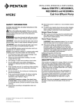
If the objects have to be deburred by hand, it can be done with several different tools,
the most common are shown in figure 4.1(a), but for manual deburring it is also possible
to use machines like the one shown in figure 4.1(b) or like the drill shown in figure 4.1(c)
and figure 4.1(d). For automated deburring it is possible to use NC/CNC machines with
all kinds of specialized deburring tools or brushes, trimming presses, edging machines for
sheet metal, end-finishing machines for tubes and bars, single purpose machines designed
for specialized deburring, gear deburring machines or robotic deburring.
4.1.1
Robot deburring
For robotic deburring, the typical applications use industrial robots to deburr large objects,
a specific part or parts of a close geometric family. Precision deburring is not preformed
9
CHAPTER 4. THEORY
10
(a) The most commonly used hand (b) Small machine for deburring and
tools for deburring
chamfering
(c) Tool mounted on a drill for chamfering/de-(d) A chamfer tool for deburring two edges
burring holes
of a workpiece
Figure 4.1: Different hand tools or machines used for deburring, either manually or automaticaly
CHAPTER 4. THEORY
11
by robots due to the fact that most of them are not capable of performing precision
movements. When robots are used to deburr large objects, the robot moves around the
object, but when deburring smaller objects with a low weight the robot moves the object
around between the tools.
Depending on the assignment, the robot should have at least 5 or 6 joints, high accuracy
and repeatability, continuous-path capability, the capability for easy and quick tool or
spindle changes, rigidity and low inertia. Extra desirable features could be easy off-line
programming, circular interpolation, and the ability to translate movements to similar
features on the same workpiece.
To achieve a good repeatability for a robot in the industry, there is a good guideline in
a combination of the following factors:
• The accuracy and positioning repeatability of the robot mechanism
• Consistency in positioning the edges of the workpiece to a reference surface (clamping
force can significantly deflect some parts)
• Nature of the edge before deburring (burr uniformity, thickness, and location consistency)
• Repeatability of the deburring tool in the robot holder
• Repeatability and accuracy of the cutting tool geometry
When working with a precision robot, the robot is often built as a point-to-point machine. Modern control methods are being used now to control robots, which leads to
continuous-path robots and controlled-path robots.
The point-to-point mode means that the robot moves from one point to another in
space with the end effector and the motion and speed of each joint of the robot cannot be
predicted. Each time a point is defined all the joint positions must be saved into a memory
block. When the robot moves, some of the joints move into position before others and
therefore the path between two points cannot be predicted easily.
Continuous-path mode means the operator is often able to grab and move the robot
from one place to another and thereby teaching the robot how to behave. Often this data
is read into a memory at continuous-time with a sampling rate from 60 to 80 Hz.
When the controlled-path mode is used, the path between each point of movement is
calculated by a computer program doing replay after the points are put into the program,
much the same way as with continuous-path robots. These points are then saved as a
location of the tool center instead of the position of each joint.
Controlled-path robots often come with one or more different interpolation types like
joint, linear, and curvilinear interpolation.
• Joint interpolation means that all the joints reach their position at the same time.
• Linear interpolation results in a linear motion of the tool center point.
CHAPTER 4. THEORY
12
• Curvilinear interpolation moves the tool center along a desired curvature.
During the actual programming of a robot, the operator can be placed next to the robot
and control the movements with a joystick or other interfaces (On-line), or he/she can
do the programming elsewhere like with a NC/CNC1 machine (Off-line). The on-line
programming is often used as a trial and error method when the robot has to work with
simple parts and the on-line programming can be used with an off-line program that needs
one or more corrections.
Using on-line programming raises some issues, like shutdown of production during programming, different equipment may block sight during programming and precision adjustments cannot be done and complex parts may be time consuming to program for precise
results. For off-line programming the operator must be able to tell the program about
weight of tools or forces done by cutting, and therefore compensate for robot arm deflections.
For robot deburring there are three philosophical approaches to accommodate for robot
inaccuracies and workpiece variations to obtain more precise results:
Compliant approach This means that the tools mounted on the robot are mounted in
a setup which adds extra compliance in one or more directions of the robot than the
robot gives. Rigidity in a setup like this is the key to success, but also fast servos
could help the system to compensate for it, but these ideal servos do not exist.
Fine-tuned robot approach This applies that the servos and resolvers have to be fine
tuned, which can increase robot accuracy by a factor of two or three. This slows down
the system a bit and also risks to put the servos in a overload position, when trying
to reach a specific position. Theoretically, this approach is the most accurate, but
due to workpiece variations, the need to minimize chatter and maximize reliability,
this approach is discarded in most scenarios. Every time something happens to the
robot, like maintenance or smaller accidents, all the programs have to be retaught
and reprogrammed.
Force feedback approach This approach is more established due to the use in other
applications, but is not used for most parts because of the difficulties to define and
control the dynamic effects. Moreover, force feedback is seen as one upcoming solution to robotic inaccuracies, workpiece tolerance variations, and incorporation of
on-line databases and off-line programming. There are four constraints preventing
the more frequent use of force feedback:
• The robotic system cannot respond quickly enough for many needs
• The dynamic response of the robot system is difficult to define for all arm
positions
1
Numerical Controled/Computer Numerical Control
CHAPTER 4. THEORY
13
• General algorithms that provide the robot logic are difficult to generalize for
three-dimensional curvilinear geometries having variable burr size and fluctuating part geometries
• Robot compliance affects sensor data
Force sensing is often used for simple tasks together with a fettling device, where the
variations of the burrs are very small and the movement is in straight lines. This
will work well as long as the burrs do not change much in dimensions. If the burrs
change, the robot does not know how the burr has changed and ends up going too
close or too far away from the workpiece leaving a mark.
Wear and tear of the tool can also change the parameters for the force sensing system.
Depending on the tool and setup used for the process, the force sensing can be used to
measure wear of the tool. This can be done by putting the tool into a hole with an
already known size and then pushing against the sides, thereby finding the size of the tool.
Comparing the new size to the one before the robot started, the process will yield the wear
of the tool. The offset is then fed into the program. A simpler method is to feed a constant
offset into the program, but the main idea is to automatically adjust to wear of the tool at
all times.
The geometric shape of the workpiece also plays a role in the deburring quality, cost,
and programming difficulty. It gets easier with more straight lines without any bending
or curves and harder if there are a lot of shallow areas, small bends, and holes in difficult
areas, which need deburring in the same process.
When a specific workpiece is the target for the operation, it must be considered whether
the robot has to handle a tool or handle the workpiece. A robot can handle a maximum
of weight at the tool tip and this confines the size of a tool or a tool together with the
workpiece. If the robot is equipped with the tool, then the workpiece has to come to the
robot on a turning table, a conveyor belt, or similiar. A fixture must lock the workpiece
in a known orientation and a change in the workpiece shape or size needs its own fixture
and more can be needed to have the robot work continuously.
If the workpiece is light, the robot will also have the possibility of lifting the workpiece
and maneuver it around between one or more fixed tools. The robot can either deliver the
workpiece to a tool or pass the workpiece over the tool tip. When the process is done the
workpiece can be passed on to another conveyor belt or the like, and the robot can grab a
new workpiece. A regrip fixture can also be put inside the workspace of the robot, to give
it access to handle all edges of a workpiece.
4.1.2
Tool Considerations
Three approaches commonly used for toolchanging are:
• Design-integral multiple motors on the end effector (at 90◦ to each other) to eliminate
the need for changing tools
CHAPTER 4. THEORY
14
• Change preset spindles
• Change grippers and tools
These approaches are used for changing the tool, when it is on the tool tip of the robot,
not changing tools in fixed tools within the workspace of the robot. When a change of
the tool is done, the motor driving the tool is often changed as well. This is easier than
designing tools for one motor unit only, if the operation of the tool is changed by the tool
change. It is often faster to make the change in the afore mentioned way.
Most tools used for manual deburring can be used for robot deburring, but a common
fact for all tools is that they will get worn out over time and therefore need to be changed
after a certain amount of runs. The deburring process will in some cases leave small burrs
and these can in some cases be minimized with a second run, see table 4.1.2, especially
when using cutters or chamfer tools.
Table 4.1: Combinations of first and second run tools appropriate for robot deburring
Subsequent
finishing approaches
Principal
Approach
Bur balls
Chamfer tools
Grinding wheels
Reverse radius cutters
Abrasive rubber
Abrasive-filled cotton
Brushing
Grinding belts
Reciprocating files
Abrasive
Rubber
Brushing
X
X
X
X
X
X
Some considerations about the optimum use of cutters:
• Correct contact point (errors often lead to vibrations)
• Correct contact angle (correct angle avoids secondary burrs)
CHAPTER 4. THEORY
15
• Correct path direction (incorrect direction of the tool motion relative to the rotation
of the tool often results in vibrations)
• Correct path velocity (depends on type of burrs, desired quality, and other factors)
• Correct resilient mounting (compliance)
Another common tool used for robotic deburring is rotating files made of high speed
steel or carbide, but these wear and also need to be changed periodically. Reciprocating or
oscillating files are also used, but do not work well together with soft metals like aluminum,
which tend to accumulate in the teeth of the file.
The deburring can also be done by abrasive-belt grinding, but here the chamfer size
is hard to control if the grinding belt is not spring or air-loaded. Furthermore, the longer
the belt is, the smaller the change in frequency. A last possibility is brushing, this leaves
a smooth blend and can remove all normal burrs. It is also easy to compensate for wear
without changing the result, because the result does not depend greatly on the applied
force.
4.1.3
Safety Considerations
When handling robots there are seven major safety hazards in robot deburring, as follows:
1. Robot runaway.
2. Inadvertent human contact with the robot.
3. Robot’s sudden release of workpiece or tooling
4. High feed rates
5. High spindle speeds
6. Noise level
7. Flying debris from broken wheels, burrs, flash, broken, wire form brushes, and sparks
from grinding.
Number 1 and 3 together can end up sending a tool or workpiece flying wildly at high
operate speeds. A high noise level may also require a walled installation to bring down
noise levels overall in the production if workers are present.
4.2
Kinematics and Mathematics
All of the mathematical and kinematic equations used in this project were researched and
established by [OI09], and therefore only a superficial explanation will be given in this
section. For further reading, [Cra04] and [OI09] are recommended.
CHAPTER 4. THEORY
16
Kinematics are the basic study of how mechanical systems behave. In this project, the
study of kinematics of robotic manipulators will refer to all geometrical and time-based
properties of the manipulator’s motion.
Kinematics are an excellent tool to obtain the position and orientation of each manipulator joint, and when used for this purpose, it is refered to as forward kinematics. Position
and orientation are determined by assigning a reference frame to each joint. A reference
frame is defined as a coordinate system with an orientation and position vector relating
the coordinate system to another frame. This is useful since it allows to describe joint positions and orientation in different coordinate systems, or a single basis coordinate system,
if desired. Six parameters are needed to describe an object: three position parameters,
and three orientation parameters. Therefore a transformation of reference frames includes
translation and rotation in one frame with respect to the other. This can be achieved
through linear algebra as described in [Eis99]. Let a x be a coordinate in base {ai } and b x
a coordinate in base {bi } then, following is valid:
ax
=a Rbb x + o x
(4.1)
where o x is a matrix defining translation from one coordinate to another, and a Rb is a
matrix that rotates from {bi } coordinates to {ai } coordinates.
In robot kinematics eq. (4.1) is usually expressed as:
·
¸ ·
¸·
¸
ax
ox
a Rb
bx
=
(4.2)
1
000 1
1
And in a simpler form eq. 4.2 can be expressed as:
ax
=a T bb x
(4.3)
Matrix a T b called the homogeneous transform and has the following property:
0T N
=0 T 1 · 1 T 2 . . .N −2 T N −1 ·N −1 T N
(4.4)
This allows the description of the position and orientation of the tool-tip on the robot
arm in the the coordinate system of the base joint. If transformation from base {bi } to
{ai } is desired, it can be done through the inverse homoegenous transform: b M a = a M b −1
4.2.1
Denavit-Hartenberg Notation
One way of expressing the forward kinematics of the robot arm is using the DenavitHartenberg notation. When talking about robot arms, two kinds of joints exist:
Prismatic joint This joint has one degree of freedom and provides sliding motion along
a single axis
Revolute joint This joint has one degree of freedom and provides rotating motion along
a single axis
CHAPTER 4. THEORY
17
Furthermore, there are four parameters defining a link (the connection between two joints):
• Link length, denoted by ai−1 , is the mutually perpendicular line between joint axes
i − 1 and i
• Link twist, denoted by αi−1 , is the angle between joint axes i − 1 and i
• Link offset, denoted by di , is a joint variable for a prismatic joint. In case a prismatic
joint is described, the other three variables will remain fixed, and depend on the
dimensions and construction of the robot
• Joint angle, denoted by θi , is a joint variable for a revolute joint. In case a revolute
joint is described, the other three variables will remain fixed, and depend on the
dimensions and construction of the robot
Ideally, any robot arm can be described by these four variables, and when done, it is
referred to as the Denavit-Hartenberg notation. A coordinate system is assigned to each
of the joints in the robot arm, this can be seen in fig. 4.2.
Figure 4.2: Denavit-Hartenberg frame assignment, taken from [MWS05]
The finer details of the Denavit-Hartenberg notation will not be explained here, for
further information refer to [Cra04] and [MWS05]. As can be seen in fig. 4.2, the Z-axis,
zi is coincident with joint axis i, the X-axis, xi , goes along the mutual perpendicular ai−1 ,
from joint axis i to joint axis i − 1, and finally, the Y-axis, Yi , is chosen according to the
right-hand rule, in order to complete the ith frame.
It is essential in the study of kinematics to be able to define frame {i} in terms of
frame {i − 1}. This transformation is usually a function of one of the joint variables
CHAPTER 4. THEORY
18
and the remaining fixed link parameters. These four variables fit into eq.(4.3), and the
homogenous transform becomes the following:


cos(θi )
− sin(θi )
0
ai−1
sin(θi ) · cos(αi−1 ) cos(θi · cos(αi−1 ) − sin(αi−1 ) − sin(αi−1 ) · di 


(4.5)
i−1 Ti = 
sin(θi ) · sin(αi−1 ) cos(θi · sin(αi−1 ) cos(αi−1 )
cos(αi−1 ) · di 
0
0
0
1
Eq. (4.5), defines the individual link transformation and accordingly, the coordinates of
the end-effector of a robot can be found by inserting eq. (4.5) into eq. (4.4), giving an
equation as a function of all joint variables.
4.2.2
Path generation
This subsection explains how a smooth path is generated between two points in spaced.
It was the method chosen in [OI09], and since this project is a continuation of [OI09], the
same method was used. A more detailed explanation can be found in [OI09]. The method
cubic polynomials is used to find the desired path from an initial position to a destination
in a certain amount of time. Four constraints are established in order to create a single
smooth motion:
p(0) = p0
(4.6a)
p(tf ) = pf
(4.6b)
d
p(0) = 0
(4.6c)
dt
d
p(tf ) = 0
(4.6d)
dt
where p0 is the start position, pf is the goal position and tf is the duration of the motion.
These constraints are satisfied by eq. (4.7a) and its derivatives:
p(t) = a0 + a1 t + a2 t2 + a3 t3
(4.7a)
d
p(t) = a1 + 2a2 t + 3a3 t2
(4.7b)
dt
d2
p(t) = 2a2 + 6a3 t
(4.7c)
dt
Solving eqs. (4.7) with the constraints from eqs. (4.6) yields the following coefficients:
a2 =
a0 = p0
(4.8a)
a1 = 0
(4.8b)
3
tf 2
(pf − p0 )
(4.8c)
CHAPTER 4. THEORY
19
a3 = −
2
(pf − p0 )
(4.8d)
tf 3
In the case a velocity limitation is needed on the motion of the end-effector, tf can be
changed from a constant to:
|pf − p0 |
tf =
(4.9)
vmax
4.3
Python programming
Python is a general-purpose high-level programming language. Its design philosophy emphasizes code readability and easy network programming. The reason Python is used as
programming language is due to the fact that the code most of this project is based upon
is already written in Python. The people behind this code have chosen the Python code
because of the easy implementation of the TCP protocol, which the UR robot uses for
communication over Ethernet. Furthermore, using this language to send commands to
the robot, allows bigger flexibility than using the GUI of the robot arm (which also allows programming to a certain degree), and simplifies the integration of the force sensor
data feedback. Another reason for using Python is the easy access to help via the internet and its similarities to other programming languages. Programming techniques learned
from the courses 02101/02102 and 310122 on JAVA and C programming give a good basic
understanding of how a programming language works, which is easily ported into Python.
4.4
Linear control
Linear control techniques were used to achieve precision in the movements of the robot.
This section explains how a proportional-integrator regulator (PI-regulator) works. The
PI-regulator has the advantage of having a good precission without the stationary error
a proportional regulator (P-regulator) produces. The transfer function (in the laplace
domain) of a PI-regulator can be seen in eq. (4.10)
¶
µ
τi s + 1
1
Gc (s) = Kp
= Kp 1 +
(4.10)
τi s
τi s
where Kp is the proportional amplification the regulation and τi is the time constant. From
the righthand-side of the equation, it is clear that the regulator consists of a proportional
amplification of the error (the Kp factor) and the integration of the error (the 1 /τi s factor).
The integrator adds a −90◦ phase-turn, and therefore an extra zero is added at s = −1
τi
[OJ06]. The control signal created by the PI-controller can also be expressed as in eq.
(4.11), which is easier to implement as an algorithm in a computer.
Z t
[htb]u(t) = Kp e(t) + Ki
e(τ )dτ
(4.11)
0
2
Both these courses are part of a group of obligatory programming introduction courses for almost all
bachelor students at DTU
CHAPTER 4. THEORY
20
Figure 4.3: A block diagram for a PI controller, note that the error is integrated and
amplified twice before it used as feedback. The reference signal is established by the
designer
Further, fig 4.3 shows the block diagram of a PI-controller. This is the structure which
will be used in this project.
The use of a proportional-integrator-differential regulator (PID-regulator), is also very
common, but has an inherent problem in the differentiation term. That is, differentiating
systems with high frequency noise, can render the whole system unstable. Therefore, this
project focuses on the use of PI-regulators.
Chapter 5
Equipment description
5.1
Force sensor
In order to measure forces at the tool tip of the robot, a Mini40 sensor by ATI Industrial
Automation is used. This sensor comes with a DAQ card1 for use in a PC. The sensor
is a transducer which together with the DAQ card, reads out 6-axis force/torque signals.
For the connection between the DAQ card and a PC an ISA port is used. An older PC
is needed to read out the force data because this form of connection is no longer used in
new PC’s. This setup means that the sensor cannot be connected directly to the robot
through the I/O interface on the robot or inside the controller to the robot, but needs to
be connected to a separate PC running Windows 2000.
The output from the sensor are 6 components, consisting of 3 forces and 3 torques (Fx , Fy ,
Fz , Tx , Ty , Tz ), which are given in a Cartesian coordinate system around the sensor, see
Appendix C.
The F/T transducer reacts to applied forces and torques using Newtons third law. The
force applied to the transducer flexes three symmetrically placed beams using Hookes law:
σ =E·ε
(5.1)
where σ, the stress applied to the beam, is proportional to the applied force, E is Young’s
modulus of the beam and ε is the strain applied to the beam.
The force sensor was calibrated before it was mounted on the robot by Ingolfsson and
Gudlaugsson [OI09]. There is no apparent reason to repeat the calibration since there has
been no observable change in readings from the sensor during tests, and the sensor is still
in the same environment2 . The sensors measuring capabilities can be seen in tab. 5.1
Ingolfsson and Gudlaugsson observed that large peak values appeared without any
force applied to the sensor except gravity. The same observation was made during this
project, but the cause of the error has not been found. This error can be disastrous for the
equipment due to high correction movements sent to the robot, depending on this reading.
1
2
Data Acquisition card
Inside a building in normal humidity and temperatures around 23 degrees Celsius.
21
CHAPTER 5. EQUIPMENT DESCRIPTION
22
Table 5.1: Metric ranges and resolution of the ATI Mini40 6-axis F/T sensor
Sensing ranges
± Fx /Fy [N]
± Fz [N]
± Tx /Ty /Tz [N/m]
40
120
2
Resolutions
± Fx /Fy [N]
± Fz [N]
± Tx /Ty /Tz [N/m]
1/400
1/200
1/16000
Therefore changes have been made to the original Python code made by Ingólfsson and
Gudlaugsson, see chapter 7 on page 32.
The graphical user interface (GUI) for the sensor output is written in Visual Basic 6
by [OI09] for the PC connected to the sensor. This program has been used without any
changes, and although only one value, Fz , was used before, attempts to use force sensing
in all three axes were made3 .
5.2
The UR-6-85-5-A robot
The Automation and Control group at DTU has received a 6-joint robot arm, from Universal Robots, in Odense, which has been made available for students to make experiments
and do project work. The model of the robot is UR-6-85-5-A and is a light robot arm,
weighing only 18 kg and capable of lifting up to 5 kg payloads. Details about the robot
can be found in the User Manual [Roba] and on the webpage www.universal-robots.com.
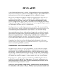
Only a quick introduction will be given here. Fig. 5.1 shows the different parts of the UR
robot:
• A: the base of the robot, where the robot is mounted
• B: the shoulder of the robot
• C: the elbow of the robot
• D,E,F: wrists 1,2, and 3 of the robot, where a tool is attached to the robot
By coordinating movement, the robot can move freely in 6 DOF with the constraints
shown in fig. 5.2, which shows that there is a cylindrical workspace along the robots base
Ẑi axis, where the tool point cannot work. Also, the figure shows that the robots working
area is a sphere of diameter 175 cm around the base.
The robot comes with a GUI called PolyScope which is easily programmable and allows
point to point movement through the definition of wavepoints. This GUI is only used in this
3
See chapter 3.2.1 in [OI09]
CHAPTER 5. EQUIPMENT DESCRIPTION
23
Figure 5.1: The links of the UR-6-85-5-A and its composition. Note that all the joints are
revolute
project to startup the robot and to log errors from the robot arm. All other programming
occurs through network protocols, as explained in sec.4.3. The GUI is a high level program
that works on top of a low level language designed by UR called URScript. This script sends
basic commands to the robot controller, like the command movej(q, a =3, v =0.75, t
=0, r =0) which receives q, a vector with six joint positions, and moves to the given
position with the acceleration a, velocity v, time t, and blend radius r.
The afore mentioned controller is a mini-ITX PC in the controller cabinet, and if
programming at script level is desired, it must occur using a TCP/IP socket connecting
to this controller from another computer. The URScript programs are executed in realtime on the URControl Runtime-Machine (RTMachine), which communicates with the
controller at a frequency of 125 Hz.
The mount flange of the robot can be seen in fig. 5.3.
Many different kinds of tools can be mounted on this flange, but for this project, only
a force sensor is mounted.
CHAPTER 5. EQUIPMENT DESCRIPTION
Figure 5.2: The workarea of UR-6-85-5-A
Figure 5.3: The mounting flange of UR-6-85-5-A
24
Chapter 6
Implementation
6.1
Analysis of Solutions
There are two different ways to approach the problem of converting the UR robot arm into
a deburring tool:
• To place a grinding machine on the end effector. This would allow the robot arm to
deburr big objects which fit into the arms working area.
• To place a gripper tool, like a suction cup, on the end effector, and pass the desired
object through deburring tools. This solution is focused on smaller objects, since the
arm can only lift up to 5 kg with precision.
A comparison of the two methods for a solution has been made in table 6.1
Each of these solutions has strengths and weaknesses, but the most important aspect
aimed at in this project is precision. If a grinding mill was to be used, the force sensor would
not be able to feel a steady push from the tool tip, since the mill would be shaving off pieces
of the object to deburr. This would mean that the amount shaved off the object to deburr
depends on the precision of movement of the robot arm and the time of displacement of
the tooltip. Since neither can be assumed to be reliable, the second method is concluded
to be the best solution, see figure 6.1. In short, the solution consists of a controlled-path
robot behaviour, combining joint and linear interpolation along with the force feedback
approach.
6.2
Method Implementation
Since this project is only a testbench, the “suction cup method” is tested, without an active
suction cup, i.e. a victim element is placed on the end effector, simulating an element which
is attached to the end effector through a suction cup, see fig. 6.2. Furthermore, the element
1
In tbl. 6.1 on the following page it is assumed that the density of steel is 7.8 g/cm3 [HDY04] and thus,
the arm is capable of lifting a square plate with a thickness of 5 mm and sides of 35 cm.
25
CHAPTER 6. IMPLEMENTATION
26
Table 6.1: Method comparisons
Tool mounted on
Workpiece mounted
end of robot
on end of robot
Weight of object
to deburr
N/A
5 Kg
Radius of arm
Depends on the weight
and size of the
object to deburr
Size of object
to deburr
Must be inside the reach
of the robot arm
Depends on the weight
of the object1
Precision of
deburr process
Depends on the odometry
of the robot arm, since
force sensor does not work
effectively with a
grinding mill.Therefore,
low precision is assumed.
Depends on the force
sensorand software code.
The forcesensor permits
adaptability,therefore,
high precisionis assumed
Not necessarily soft
metals like aluminium
All kind of materials
as long as a gripper
can be designed
Highest
Higher than most machine
or hand deburring processes
Reach of robot arm
Strength of
material
Speed
holders will not be built, but it is assummed that all elements are picked up at the exactly
same position with the same rotation.
For the proof of concept, it is assumed that the robot is standing in a production line
where it has to deburr metal plates with the dimensions 10 cm × 15 cm Figure 6.3 shows
a flowchart of how the robot deburrs all four sides of the elements. An element has been
mounted on the existing tool of the robot from the project [OI09]. The idea behind this
setup is to simulate a deburring process of four sides of this element in a model of a setup
around the robot. For this setup a model has been drawn for a deburring platform, see
appendix E on page 62. With help from the AUT department, this model was made in
wood and mounted within the workspace of the robot. The model was mounted on a small
table next to the robot in the lab, with clamps to prevent it from moving when the robot
pushes the victim element against it. The robot was programmed to simulate the process of
picking up the element, deburring its four sides, and then delivering the element for further
work elsewhere. The programming for this task will be discussed in chapter 7 on page 32.
The tool chosen to be simulated is like the one in figure 4.1(b). The size of the tool is
determined depending on the size of the element, which in this case is 10 cm × 15 cm, but
the size of the tool can easily be changed if the size of the workpiece should be changed. It
CHAPTER 6. IMPLEMENTATION
Figure 6.1: A simplified model of the theoretical setup of the deburring process
Figure 6.2: Test bench setup with an element attached to the robot tooltip
Figure 6.3: A flow chart of the deburring process
27
CHAPTER 6. IMPLEMENTATION
28
should be kept in mind that the size and speed of the cylinder doing the deburring depends
on which material it should work on, how much material it should remove and how fine
the result should be.
Appendix D on page 60 also shows a sketch of the victim element mounted on the
robot. The mounting between the element, sensor and the robot is not included, since
it was already made before this project started. The element ends up being mounted
approximately 10 cm from the center of the tool tip2 of the robot.
6.2.1
Deburr Process
The movements, before and after the element is near the deburring machine, are easy to
program as point to point movements. This also includes the rotation of the victim element
to change side for deburring, and the position before the deburr process is started. While
the robot is to collect or deliver an element, the force sensor is used to make sure that
the robot is pushed against the element or the element underneath before a vacuum is
activated or deactivated if a suction cup was implemented.
The elements ready to be picked up by the robot are to be placed in a holder where the
elements are fixed in a precise position. In this way, the robot always picks up an element
in almost the same position. Due to programming, a small deviation of ±1 mm in this
position is allowed. The position of the holder for unloading the plates does not have to be
in a fixed position either. The holder is allowed to deviate in both rotation and position
by ± 1 mm.
In the position for deburring, no matter which side of the element is chosen for deburring, force measurements must be used for impact control and regulation. First, impact
control must be used to make the element move all the way to touch the deburring tool
in two directions. The robot is programmed to move towards the deburring tool in one
direction, the Zs -direction of the force sensor, see fig. 6.4. This corresponds to a continous
movement along the Xr -axis and −Zr -axis of the robot, until the force sensor measures a
given reference value.
To complete the positioning of the element before the actual deburring is done, contact
has to be made with the rest of the sled of the deburring setup. This is completed by
moving the plate a 5 mm away from the machine and approaching the sled in the force
sensor’s −Xs -direction, which correspond to the −Xr -direction and −Zr -direction of the
robot, until a force reference value is reached once more. Then the approach in the force
sensor’s Zs -direction is called once more to make the plate reach the sled as close as possible.
Fixed in the sled, the element is ready to be run by the deburring mill, which means the
element is moved along the robots Yr -axis, while it is pushed against the tool sled in the
force sensor’s Zs - and Xs -direction. The movement is controlled by a PI-regulator trying
to maintain a constant force in the Zs -direction. Position regulation along the Xr and Zr
axes is desired, and two PI-regulators maintain the wanted position along these two axes.
When one side has been deburred, the robot deburrs three more sides before it is done
2
TCP, Tool Center Point, named by UR
CHAPTER 6. IMPLEMENTATION
29
Figure 6.4: Model of approach to deburr tool. The Yr and Ys axis are chosen according to
the right hand rule. A spindle is
and ready to drop off the victim element again. In a production line, the element would
be turned upside down at the drop off point and put trough the process once more to
deburr all eight edges, but this is outside of both our time line and main problem, and will
therefore be saved for future work.
6.2.2
Linear control design and kinematic values
The regulation used for the project was based on the hybrid-control used in [OI09]. Fig.
6.5 shows a general block diagram of how the desired regulation is achieved. The ideal
solution for the deburring process would have force regulation between the victim element
and the deburr platform on the robot’s Xr and Zr axes, see fig6.4.
The resulting system to be regulated would be of the multiple-input/multiple-output
(MIMO) kind. This fact, paired up with torques and forces generated on the force sensor
due to torsion when the victim element is not exactly aligned with the deburring sledge,
results in the need of complicated regulation. The needed regulation is taught at DTU as
part of a masters course, and due to limitations on time, a simpler solution is chosen. The
regulation solution will have the following properties:
• Force feedback and regulation in the robot’s x- and z-axis
• Position feedback and regulation in the robot’s y- and z-axis
• A hybrid force/position regulation scheme
• A slightly underdamped system, which gives a better result
CHAPTER 6. IMPLEMENTATION
30
Figure 6.5: Block model of a hybrid force/position control scheme from [OI09]. Note that
the forward kinematics are used to transform the joint positions θi to Cartesian coordinates,
which are used as feedback for the position controller.
This regulation was achieved in the draw function of the python code, see chapter 7
on page 32 for more information. The tuning of the values Kp and Ki was made by hand,
trying different values, although the initial values were found using the Ziegler-Nichols
criteria, as described in [OI09].
The values for the Denavit-Hartenberg notation used are shown in table 6.2 The values
are then inserted into the homogenous transform as stated in chapter 4.2 on page 15, and
using eq. (4.4) the homegenous transform 0 T 6 , which will be used in the programming for
movement and location of the robot.
CHAPTER 6. IMPLEMENTATION
31
Table 6.2: Denavit-Hartenberg values used for the robot. They are obtained through
measurements made on the robot arm
i(frame) αi − 1 [◦ ] ai − 1 [m] di [m] θi
1
0
0
0.0892
θ1
2
90
0
0.1357
θ2
3
0
-0.42500
-0.1357
θ3
4
0
-0.39243
0.1090
θ4
5
90
0
0.0930
θ5
6
-90
0
0.0820
θ6
Chapter 7
Programming the robot
7.1
Functions and their uses
The code for this project builds upon the program from an earlier project, [OI09]. After an
analysis of this code, functions which were needed to complete the task had to be written
or modified. Afterwards, all the functions which were no longer in use had to be erased.
The purpose of the new functions are described on the flowchart in figure 6.3 on page 27.
These functions created with Python work as a high level programming language working on top the URScript. There are two classes which were made:
• The force class, containing functions designed to retrieve information and remove
bias from the force sensor F.0.3
• The connection class, containing functions designed to speak with the robot, and
thus send all movement scripts to the robot F.0.2
These two classes each have their own file, and a third file, called maindeburr.py F.0.1,
serves as a primitive GUI. These three files can be seen in Appendix F, and can be analyzed
if a detailed understanding of the different classes and functions is desired.
Mainly five kinds of tasks need to be scripted in order to do the deburring work:
Large movements in workspace These movements are made by establishing waypoints
where the robot arm has to stop. These points are called through the movej command1
Approach with sensor feedback These functions were made by having loops moving
the tooltip in a desired direction, with the speedl script, while comparing the data
of the force sensor to a given reference value. In most cases this reference value was
4 N. This kind of function is also used to simulate the pickup and delivering of the
elements to be deburred
1
For specific details on the working of these commands, refer to URscript Manual [Robb]
32
CHAPTER 7. PROGRAMMING THE ROBOT
33
Decoupling movements These movements are made with the speedl script, moving only
short distances away from the deburr setup. The original script was made by Ingólfsson and Gudlaugsson, but this function is now divided into two different scripts,
decoupling on different axes
Rotation of the tool point This is achieved by logging the current position of the joints
and then using the movej script to rotate wrist 3 of the robot. The rotation is made
with a slight bias due to the general position of the robot arm relative to the setup
Translation of the tool point with force regulation activated This is the most important movement of the project, since it is the one that defines the precission of the
deburr work. This movement was achieved by creating a path, as described in chapter
4.2.2, and continously sending the information from the force sensor and the position feedback through the PI-regulators. This was done in the draw function of the
connection class. The position feedback uses the forward kinematics in order to find
the Cartesian coordinates from the data received by the robot.
Since the victim element at the tool point creates a force bias due to gravity, the force
sensors bias needs to be removed after most of the movements are completed. This function
is defined in the force class.
Some of the used functions were already written by Ingolfsson and Gudlaugsson. But
many of them are partially or completely rewritten in order to fit into this project, e.g. the
original approach function only moved in the Zs direction, parallel to the Xr -axis, while
the rewritten one moves in a combination of Xr and Zr axes. The source code has been
commented in order to make clear which functions are based on Ingólfsson et. al. original
functions.
Two python-modules are loaded into the program: numpy and socket. Numpy, or
numerical python, is in charge of the mathematics and creating different matrices. Socket
is in charge of TCP communication with the robot controller, and adding this module allows
to functions like socket.rcv and socket.send to be called. It is mainly due to the capabilities
of this module that python was chosen as the programming language by Ingolfsson and
Gudlaugsson.
7.2
User manual for the program
To start up the program, it should first by assured that the robot, user-pc and sensor-pc
are connected and are on the same network.
The IP-settings for the robot should be: IP:192.38.66.237 Subnet: 255.255.255.0, the
IP-settings for the user-pc should be: IP:192.38.66.x2 Subnet: 255.255.255.0, and the IPsettings for the sensor-pc should be: IP:192.38.66.252 Subnet: 255.255.255.0. Control the
connection between the sensor and the sensor pc is plugged in correctly.
2
x should be a number between 1-255, except 252 and 237
CHAPTER 7. PROGRAMMING THE ROBOT
34
Then the Visual Basic 6 script written for [OI09] on the sensor PC should be started,
press the following buttons: Listen, Initialize sensor, Remove bias, and Fetch data. The
last one is to check that everything is working, and if the data is not close to zero it might
suggest an error.
Turn on the robot, follow the text on the screen to initialize it. Remove anything
withing 20 cm of the robot arm before turning the power on and be careful not to hit
anything while moving the arm, during this stage.
When the robot is initialized, choose “Program Robot” on the main screen and go to
the Log tab. This will help understanding any problem, if one should occur. Make sure
the Ethernet controller does not have packet loss at this stage, otherwise restart the robot
right away. Now it is possible to start the user interface at the user-pc. Make sure that
the user-pc has Python version 2.5 and the source code from this project. Start the file
called maindeburr.py from Appendix F.0.1, on Microsoft Windows 2000 or newer. This
can be done by a double click on the file or by running the file in a command window. In
Unix/Linux systems it can be run in a terminal window.
The program will start moving the robot to the first position and when it is done, the
main screen will show, see figure 7.1. The following choices are possible:
deburr Choosing this will make it possible for the user to choose how many elements to
deburr and then start the process. The maximum number of elements is 10 pieces.
debug Choosing this will make it possible for an advanced user to access the temporary
menu, used to do the programming. This menu is partly a copy of the one use by
[OI09] with a few extra options
exit Choosing this will shut down the program, after closing any open files or sockets
Figure 7.1: Mainscreen for the user interface at the user pc connected to the robot controller
and sensor pc
Before any use of the robot always read the safety instruction in the user manual for the
robot [Roba].
Chapter 8
Calibration and Test
This chapter shows how the solution for the given problem was tested and how the instruments were calibrated in order to get precise and accurate measurements. Further, the
collected graphs and data, are discussed and compared.
8.1
Test of communication speed
Ingólfsson and Gudlaugsson observed that communication over Ethernet between the control PC, sensor PC and the robot not always worked as described in the data sheet of the
robot. The sensor PC did not show problems of communication, due to the fact that it
does not communicate with the robot, but only with the sensor and the control PC. A
model of the network can be seen in figure 8.1.
In the script manual [Robb] of the robot it is stated that the robots real time RuntimeMachine1 can handle communication at a speed of 125 Hz. This frequency has proven
to be difficult to mantain while running communication over Ethernet. The robot crashed
with the error “No Controller” 2 and stopped if calls were sent at this rate. By restricting
the send rate to 41 Hz, the crash error was prevented from occurring everytime. This crash
error still appears sporadically, without any clear reason.
To test the controller crash problem, a small piece of code was designed to call one of
the UR Script commands at a determined rate. This also gave an opportunity to learn
move about the UR Script. The random() command was chosen, because the robot does
not have to move for this command to work and thereby does not have to ensure that it
always stays inside its own workspace. This command is also supposed to return a value
to the control PC, like most of all other commands that move the robot.
This small program consist of a “while” loop, where the speed of the loop can be
controlled to determine the frequency of the call of the socket.send() command. The idea
was then to run the loop at different frequencies and see how long it would run without
1
2
See chapter 5.2 on page 22
In the log: PolyScope disconnected from Controller
35
CHAPTER 8. CALIBRATION AND TEST
36
Figure 8.1: A model of the network around the robot
getting the error on the touchscreen of the robot. To determine if this command actually
reached the robot and the robot answered, a program was included in the loop, which wrote
the answer from the robot with a time stamp to a file. This file did work, but the answer
from the robot was not as expected, since it consisted of the position of the robot and not a
random number from 0-1 as the UR Script manual stated. Also, the time stamp to control
the frequency in the text file was not working as planed and needed reprogramming to be
sure it was accurate.
Due to the failure of completion of this test, the project was continued with restrictions
on the communication speed. This means that when a movement is done which depends
on a read-out from the force sensor, the frequency for every socket.send() command call to
the robot is locked to 41 Hz, as in [OI09].
The only function not having the same frequency restriction is the approach_z_x, which
has even more strict limitations on the speed of the socket.send() calls.
8.2
Force feedback during deburr
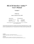
The read-out of the force sensor was logged for analysis purposes and can be seen in fig.
8.2.
From this graph, it is clear that regulation toward a force reference of 4 N is achieved.
The graph shows the force feedback each time a side of an element is passed through
the deburr setup. It is also quite clear here, that the force regulation is very sensitive
CHAPTER 8. CALIBRATION AND TEST
37
16
14
Actual Force
Reference Force
12
10
Z [N]
8
6
4
2
0
−2
0
10
20
30
Time
40
50
60
Figure 8.2: Force feedback during the deburring of the four sides of an element. The first,
third and fourth deburr maintain a stable pressure agains the deburr sledge
to the start position of the robot, and whether the victim element is completely aligned
with the debur sledge or not. The first, third and fourth runs maintain an even force
regulation, while the second loses its grip against the deburr sledge. This happens because
the alignment angle between the sledge and element is too big when the element is rotated
into the second position for deburring. This could be solved by having a tool tip which is
able to bend and adapt a few degrees, so the plate ends up being completely flat against
the deburr sledge.
8.3
Noise on the force sensor
The force sensor used in this project has been described in chapter 5.1 on page 21 and
it has been noted that it had an unpredictable error, which showed as a a peak read-out
of a force larger than what the sensor should be able to measure. In the Appendix A on
page 46 sets of data are listed, containing information read out from the force sensor in
nine different positions in the workspace of the robot:
• Random position
• Deburr positions 1 − 4, just before the robot starts moving towards the deburr setup
• Initialize position
• Stretched out horizontal, with the tool at maximum reach, downward, and upward
CHAPTER 8. CALIBRATION AND TEST
38
First deburr position
0.6
Force on the Z−axis [N]
Actual F.
Reference F.
Maximum & Minimum
0.4
0.2
0
−0.2
Force on the Y−axis [N]
Force on the X−axis [N]
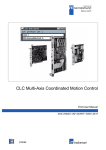
In each data set there are values which are out of the measuring range of the force
sensor. It should be noted that the sensor cannot measure more than ±40 N of force in
the x-axis and y-axis, and ±120 N of force in the z-axis, see table 5.1 on page 22. The
data received reaches numbers up to ±255 N or even ±256 · 108 N, and this error is not
connected to only one axis.
These peak errors have to be removed from the data sent to the system, otherwise the
corrections for the robots movements can be fatal for the equipment and setup. Still, the
setup has completed the deburr process of 10 elements in a row without crashing or having
serious errors.
2
Actual F.
Reference F.
Maximum & Minimum
0
−2
−4
0.3
Actual F.
Reference F.
Maximum & Minimum
0.2
0.1
0
−0.1
0
500
1000
1500
Sample point
Figure 8.3: Graphic representation of noise recieved on the force sensor, when the robot is
in the first deburr position, see also Appendix A
With the high peak errors removed from the data sets, the force sensor still experiences
errors, but smaller than ±2 N. This can be seen in figure 8.3. The figure show force
measurements from all three axis at the moment where the robot is at a waypoint, just
before it starts deburring the first edge of an elelement.
If these numbers are compared to the rest of the measurements in the Appendix A
it is apparent that the force sensing depends on when exactly the force bias is removed
from all three axis. It is concluded that the measured noise comes from the robot. While
standing still in a position in space and turned on, the robot will always vibrate a little
and this movement is measured by the force sensor. The vibrations come from the motors
in the robot, which are trying to hold the robot still in the preprogrammed position while
working against gravity. The hight vibration measurements are due to the weight of the
element at the tool tip, which amplifies the error readings at the sensor.
CHAPTER 8. CALIBRATION AND TEST
39
When the robot moves there is also noise on the sensor, but this phenomenon has not
been analyzed in this project. When the force sensor is used throughout this project, the
noise coming from the vibrations of the robot has been discarded as always being within a
margin of ±4N during a move through the deburr tool. This can be seen in section 8.2 on
page 36. During the project, this noise has been taken into account regarding the linear
control, which led to the use of a PI-regulator instead of a PID-regulator3 .
In [OI09] noise problems were minimal due to the small weight of the tool on the tip of
the sensor. This noise was not taken into account since most of the noise came from the
contact point between the chalk and the surface of the chalkboard or between the peg and
the block of tree with a hole.
3
See chapter 4.4 on page 19
Chapter 9
Errors in the robot
The robot used in this project is a prototype model used for tests inside UR. This means,
it was built as one of the first of its type and some parts of the robot and its controls may
have changed in newer version. This section will explain some of the problems which were
encountered throughout this project.
When the robot is being turned on for the first time after long period of inactivity, it
does not always work and needs to be restarted. The error consists in some kind of failure
in the Ethernet card or driver, which does not start up the Ethernet properly. The log
states “Ethernet 001 Packets loss”, which does not explain much, but implies that the error
lies in the network communication drivers of the robot.
Another error comes after the control box for the robot has been moved. The wires for
the touchscreen might be moved as well and an error occurs with the touchscreen, making
it impossible to control the robot without an external mouse or keyboard. This error has
not been present all the time, but appears due to wear and tear on the wires which go into
the control box. When these wires were installed at UR, nothing was used to prevent the
sharp edges of the control box to cut into the wires, and if a closer look is taken, it is now
possible to see through most of the isolation cap and into the cores or shields of almost all
the wires.
This model was not meant to be transported, moved or placed in an environment which
vibrates in any way. This limitation has not been commented to the AUT group, or any
student working with the robot. The limitation became apparent when the log suddenly
one morning simply stated “48 V Internal power supply is at 0V” at start up. The robot
had the day before shown no problems when turned off. Universal Robots was contacted
and the problem was explained. The solution was that the control box should be taken
apart an examined at DTU, rather than sending it to Odense and back, which could have
taken weeks off the projects time schedule.
When taken apart, it was clear what was wrong: one wire from the 48 V Internal power
supply had been torn out from its socket on the main controller board. This apparently
happened due to the length of the wire and vibrations between the power supply and the
main controller board. While the controller was taken apart it was also noted that two
out of three ceramic resistors had almost broken completely off. This also occurred due to
40
CHAPTER 9. ERRORS IN THE ROBOT
41
vibrations, and because the resistors had not been mounted correctly, but had only been
installed in a socket in one end. The weight of each resistor had then been enough to move
it around every time the controller box was shaken or moved due to gravity. After some
time, the wires connecting the resistances must have become weak and broken off.
Representative of UR stated that the resistors are used to burn off energy when the
robot is deaccelerating and no damage should have been done as long as the robot had not
been used intensively over a long period. Two new resistors were sent from Odense and
installed upon arrival, this time secured by strips to avoid the same error again later on.
UR claims that this construction error has now been corrected.
In section 8.1 on page 35 an error concerning the controller crashing has been explained.
During the project, this error has appeared on different occasions, and was mentioned to
UR. It was discussed if the heat that building up inside the controller box could affect the
controllor. UR insisted that is was not the case, because the temperature should not rise
above the maximum working temperature for all the components inside the controller box.
Chapter 10
Conclusion
Throughout the realization of this project, several branches of engineering and tools have
been used. Programming, linear control, physics and mathematics are among the most
prominent, and they were all used together to achieve a result. This result is the creation
of a test bench which proves that a robot arm UR-6-85-5-A is able to deburr four sides of
a metal plate (victim element) using a force sensor installed on its tool tip. A setup was
created to simulate the deburring process, which is divided into the following steps:
1. The user chooses how many elements are to be deburred
2. The robot arm simulates picking up an element with a suction cup
3. Using force regulation in order to follow a surface, the robot passes the victim elements four sides by a mock-up of a deburring machine
4. The robot arm simulates delivering the deburred plate at a given position
5. The robot repeats the procedure if necessary
Programming was made with the Python language, and proved to be very effective to the
task. It eased the use of the URScript language and communication with the robot arm.
Force regulaton was achieved through the use of a PI-regulator acting in the software. It
regulated along the Z-axis of the sensor, and proved to be moderately adequate for the
task. Other control techniques might have been better for force regulation in two axes, but
knowledge of those techniques was outside the scope of this project.
The solution is not as precise as it was hoped it could be. This stems from the fact that
only force regulation in one axis was achieved. At the same time, a solution was expected
to be found for removing/dampening the vibrations generated by the robot, but they only
became worse due to the heavy weight on the tool tip.
The team is satisfied with the knowledge acquired during this project, and with the results
achieved.
42
Chapter 11
Future Work
Throughout this project, more problems have been revealed during the search for solutions
to the stated questions in the problem statement. Some of these have been outside the
frame of this project, others were too time consuming, and some have had to be discarded
due to the lack of the knowledge needed to solve the problem.
The following points are tasks or problems which could be solved in the future as a
special course, or simply for the challenge:
Change in size of the elements to be deburred The product of this project can be
made to take an input of the dimensions of the victim elements and thereby adjust
all the waypoints in the procedure to take the dimensions into account before moving
from waypoint to waypoint
Improving the use of the deburr tools As described in 4.1 on page 9 the wear and
tear on the deburr tool will make the deburring less precise for every run, and at
some point the tool needs to be sharpened or replaced. When a tool has been chosen,
the amount runs before the tool needs to be changed has to be determined, if the tool
manufacturer has not stated this already. A solution to extend the life of a tool can
be to made through a mechanism that moves the angle of attack on the tool between
or during each run
Deburring all eight sides of an element Another future feature can be to design a
regrip fixture for the setup inorder to make the robot capable of deburring all eight
edges of a victim element
Expansion of the control to force feedback in several axes The SISO system developed in this project can be optimized into a multiple input/multiple out (MIMO)
system that is able to use force feedback from all axes of the sensor or even the torque
outputs. This would make the victim elements follow all the sides of the modelled
deburr tool even smoother
Noise reduction A filtering system can be built inorder to remove even more noise from
the force sensor at the TCP of the robot. This would make the controlled movements
43
CHAPTER 11. FUTURE WORK
44
even smoother
Completion of test setup The setup can be completed adding a suction cup at the tool
tip and a vacuum system mounted near the robot. Also the holders beside the robot
for the arriving and leaving victim elements can be designed and put into the setup.
A real grinding mill could be installed too, although some security measure should
be established
Bibliography
[A.] ATI
I.
A.
Mini40-r.
On-line,
ia.com/products/ft/ft_models.aspx?id=Mini40.
http://www.ati-
[Cra04] John J. Craig. Introduction to Robotics - Mechanics and Control. Prentice Hall,
3rd edition, 2004.
[CW76] Raymond F. Veilleux Charles Wick. Tool and Manufacturing Engineers Handbook: Materials, Finishing, and Coating, volume III, chapter 16. McGraw-Hill
Book Co., 1976.
[Eis99] Jens Eising. Lineaer Algebra. Institut for Matematik, DTU, 1999.
[Gil99] LaRoux K. Gillespie. Deburring and edge finishing handbook. Asme Books, 1999.
[Har] Tom Harris.
How robots work.
How Stuff Works.
http://science.howstuffworks.com/robot2.htm.
On-line,
[HDY04] Roger A. Freedman Hugh D. Young. University Physics with Modern Physics,
chapter 14, page 516. Pearson Addison Wesley, 11 edition, 2004.
[Iso05] James Isom.
A brieg history of robotics.
http://robotics.megagiant.com/history.html, 2002-2005.
On-line,
[MWS05] Mathukumalli Vidyasagar Mark W. Spong, Seth Hutchinson. Robot Modeling
and Control, chapter 3, page 496. Wiley, 2005.
[OI09] Einir Gudlaugsson Örn Ingólfsson. Flexible control of a robot arm using sensor
feedback. Master’s thesis, DTU Electrical Engineering, July 2009.
[OJ06] Paul Haase Soerensen Ole Jannerup. Reguleringsteknik. Polyteknisk Forlag, 4th
edition, 2006.
[Roba] Universal Robots. UR-6-85-5-A Users Manual. Universal Robots, On-line
(PDF), http://www.universal-robots.com/, 1.1 edition.
[Robb] Universal Robots. The URScript Programming Language. Universal Robots,
On-line (PDF),www.universal-robots.com.
45
Appendix A
Force error on the axes
46
APPENDIX A. FORCE ERROR ON THE AXES
2
0
−2
−4
2
1
0
Force on the X−axis [N]
−1
1
0.5
0
−0.5
Force on the Y−axis [N]
−2
Force on the Z−axis [N]
47
0
Sample point
Random position of the robot
500
1000
1500
Actual F.
Reference F.
Maximum & Minimum
Actual F.
Reference F.
Maximum & Minimum
Actual F.
Reference F.
Maximum & Minimum
Figure A.1: Graphic representation of noise received on the force sensor, when the robot
is in a random position
APPENDIX A. FORCE ERROR ON THE AXES
Force on the Z−axis [N]
48
Force on the X−axis [N]
0.6
0.4
0.2
0
−0.2
2
0
−2
−4
0.3
0.2
0.1
0
−0.1
Force on the Y−axis [N]
0
500
First deburr position
Sample point
1000
1500
Actual F.
Reference F.
Maximum & Minimum
Actual F.
Reference F.
Maximum & Minimum
Actual F.
Reference F.
Maximum & Minimum
Figure A.2: Graphic representation of noise received on the force sensor, when the robot
is in the first deburr position
APPENDIX A. FORCE ERROR ON THE AXES
Force on the Z−axis [N]
49
Force on the X−axis [N]
1
0
−1
−2
−3
0.4
0.2
0
−0.2
−0.4
0.1
0.05
0
−0.1
−0.05
Force on the Y−axis [N]
0
Sample point
Second deburr position
500
1000
1500
Actual F.
Reference F.
Maximum & Minimum
Actual F.
Reference F.
Maximum & Minimum
Actual F.
Reference F.
Maximum & Minimum
Figure A.3: Graphic representation of noise received on the force sensor, when the robot
is the second deburr position
APPENDIX A. FORCE ERROR ON THE AXES
Force on the Z−axis [N]
50
Force on the X−axis [N]
0.2
0
−0.2
−0.4
−0.6
2
0
−2
−4
0.2
0.1
0
−0.1
−0.2
Force on the Y−axis [N]
0
500
Third deburr position
Sample point
1000
1500
Actual F.
Reference F.
Maximum & Minimum
Actual F.
Reference F.
Maximum & Minimum
Actual F.
Reference F.
Maximum & Minimum
Figure A.4: Graphic representation of noise received on the force sensor, when the robot
is in the third deburr position
APPENDIX A. FORCE ERROR ON THE AXES
Force on the Z−axis [N]
51
Force on the X−axis [N]
2
0
−2
−4
0.6
0.4
0.2
0
−0.2
0.1
0.05
0
−0.1
−0.05
Force on the Y−axis [N]
0
500
Fourth deburr position
Sample point
1000
1500
Actual F.
Reference F.
Maximum & Minimum
Actual F.
Reference F.
Maximum & Minimum
Actual F.
Reference F.
Maximum & Minimum
Figure A.5: Graphic representation of noise received on the force sensor, when the robot
is in the fourth deburr position
APPENDIX A. FORCE ERROR ON THE AXES
Force on the Z−axis [N]
52
Force on the X−axis [N]
0.2
0
−0.2
−0.4
−0.6
2
0
−2
−4
0.2
0.1
0
−0.1
−0.2
Force on the Y−axis [N]
0
500
Init position
Sample point
1000
1500
Actual F.
Reference F.
Maximum & Minimum
Actual F.
Reference F.
Maximum & Minimum
Actual F.
Reference F.
Maximum & Minimum
Figure A.6: Graphic representation of noise received on the force sensor, when the robot
is in the initialize position
APPENDIX A. FORCE ERROR ON THE AXES
1
0
−1
−2
2
0
Force on the X−axis [N]
−2
0.5
0
−0.5
Force on the Y−axis [N]
−4
Force on the Z−axis [N]
53
0
Sample point
Horizontal stretch of the robot
500
1000
1500
Actual F.
Reference F.
Maximum & Minimum
Actual F.
Reference F.
Maximum & Minimum
Actual F.
Reference F.
Maximum & Minimum
Figure A.7: Graphic representation of noise received on the force sensor, when the robot
is in a horizontal stretched position with the tool pointing outward
APPENDIX A. FORCE ERROR ON THE AXES
3
2
1
0
−1
2
1
0
Force on the X−axis [N]
−1
0.6
0.4
0.2
0
−0.2
Force on the Y−axis [N]
−2
Force on the Z−axis [N]
54
0
Horizontal stretch of the robot, the tool turned downward
500
Sample point
1000
1500
Actual F.
Reference F.
Maximum & Minimum
Actual F.
Reference F.
Maximum & Minimum
Actual F.
Reference F.
Maximum & Minimum
Figure A.8: Graphic representation of noise received on the force sensor, when the robot
is in a horizontal stretched position with the tool pointing downward
APPENDIX A. FORCE ERROR ON THE AXES
2
1
0
−1
2
1
0
Force on the X−axis [N]
−1
0.5
0
−0.5
Force on the Y−axis [N]
−2
Force on the Z−axis [N]
55
0
Horizontal stretch of the robot, the tool turned upward
500
Sample point
1000
1500
Actual F.
Reference F.
Maximum & Minimum
Actual F.
Reference F.
Maximum & Minimum
Actual F.
Reference F.
Maximum & Minimum
Figure A.9: Graphic representation of noise received on the force sensor, when the robot
is in a horizontal stretched position with the tool pointing upward
Appendix B
CD List of Contents
9230-05-1278.pdf Drawning of the Mini40-R force sensor
BondyS051976-WahlgreenS042157.pdf Copy of the report with signatures
connectionregulatortest.py Program for all communication between the user-pc and
the robot controller
Drawing - deburr.igr Drawing of the model of the deburr tool, opens in SmartSketch
Drawing - deburr.pdf Drawing of the model of the deburr tool
Drawing - tool.igr Drawing of the victim element, opens in SmartSketch
Drawing - tool.pdf Drawing of the victim element, opens in SmartSketch
force.py Program for all communication between the user-pc and the sensor-pc
force_test.py Test program, which reads out data from the sensor for analyze
force_test.txt Test data from force sensor, random position
force_test_deburr1.txt Test data from force sensor, 1( st) side position
force_test_deburr2.txt Test data from force sensor, 2( nd) side position
force_test_deburr3.txt Test data from force sensor, 3( rd) side position
force_test_deburr4.txt Test data from force sensor, 4( th) side position
force_test_init.txt Test data from force sensor, init position
force_test_stretch.txt Test data from force sensor, horizontal stretch of robot with
tool at maximum range
force_test_stretch_down.txt Test data from force sensor, horizontal stretch of robot
with tool downward
56
APPENDIX B. CD LIST OF CONTENTS
57
force_test_stretch_up.txt Test data from force sensor, horizontal stretch of robot
with tool upward
maindeburr.py Main program file
scriptmanual_en.pdf URScript Manual from UR
testit_fourthrun.txt Test data from force sensor, while deburring one element
UR-6-85-5-A_Produktblad_web_UK.pdf Datasheet for the UR–6–85–5–A
Appendix C
Drawing of force sensor
58
APPENDIX C. DRAWING OF FORCE SENSOR
Figure C.1: Technical drawing of the force sensor [A.]
59
Appendix D
Drawing of the victim element
60
APPENDIX D. DRAWING OF THE VICTIM ELEMENT
Figure D.1: Technical drawing the victim element, Not in scale, see B
61
Appendix E
Drawing of the deburr tool model
62
APPENDIX E. DRAWING OF THE DEBURR TOOL MODEL
Figure E.1: Technical drawing no. 1 of the deburr tool model, Not in scale, see B
63
APPENDIX E. DRAWING OF THE DEBURR TOOL MODEL
Figure E.2: Technical drawing no. 2 of the deburr tool model, Not in scale, see B
64
Appendix F
Source code
F.0.1
maindeburr.py
# −∗− c o d i n g : cp1252 −∗−
d e f s y s t e m c l e a r ( ) : #This c l e a r s t h e s c r e e n depending on t h e OS used
import os
i f os . name == " p o s i x " :
# Unix / Linux /MacOS/BSD/ e t c
os . system ( ’ c l e a r ’ )
e l i f os . name i n ( " nt " , " dos " , " c e " ) :
# DOS/Windows
os . system ( ’ CLS ’ )
import numpy
from numpy import ∗
import time
import l o c a l e
l o c a l e . s e t l o c a l e ( l o c a l e .LC_NUMERIC, ’ ’ )
from c o n n e c t i o n r e g u l a t o r t e s t import Connection
from f o r c e import Force
c = Connection ( ’ 1 9 2 . 3 8 . 6 6 . 2 3 7 ’ , 30003)
t = 0
w h i l e ( t ==0):
systemclear ()
p r i n t "Moving r o b o t i n t o s t a r t p o s i t i o n , p l e a s e wai t "
c . i n i t i a l i z e ()
systemclear ()
f = Force ( ’ 1 9 2 . 3 8 . 6 6 . 2 5 2 ’ , 12345)
f . bias ()
c . init_variables (4 ,0.02 ,0.0005 ,1)
65
APPENDIX F. SOURCE CODE
66
plates = 1
p r i n t ""
p r i n t "#################################"
p r i n t "###
Welcome t o
###"
p r i n t "###
t h e deburr program
###"
p r i n t "#################################"
p r i n t ""
p r i n t "The commands f o r t h i s program a r e : "
p r i n t " d eb urr =
Start deburring "
p r i n t " debug
=
Enter debug menu"
print " exit
=
E x i t t h e program "
p r i n t ""
p r i n t " I f no o r a wrong i n p u t i s g i v e n "
p r i n t " you w i l l r e t u r n t o t h i s s c r e e n "
p r i n t ""
c h o i c e = raw_input ( "Command : " )
p r i n t ""
i f c h o i c e == " deburr " :
p l a t e s = raw_input ( "How many p l a t e s s h o u l d be deburred ? (MAX 1 0 ) : " )
try :
plates = float ( plates )
e x c e p t Exception , e :
p r i n t " E r r o r ! " , e , " P l e a s e make s u r e you put i n a number between 1−1
e x i t ( " \ nTry s t a r t i n g t h e program a g a i n \n " )
i f plates > 10:
p r i n t ""
p r i n t "#################################"
p r i n t "###
Deburring p l a t e s 10
###"
p r i n t "#################################"
p r i n t ""
p l a t e s = 10
e l i f p l a t e s <= 0 :
p r i n t ""
p r i n t "#################################"
p r i n t "### NOT Deburring any p l a t e s ###"
p r i n t "#################################"
p r i n t ""
time . s l e e p ( 3 )
deburred_plates = 0
systemclear ()
while deburred_plates < p l a t e s :
p r i n t ""
APPENDIX F. SOURCE CODE
67
p r i n t "#################################"
p r i n t "###
P l a t e no %s i s runni ng
###" % s t r ( d e b u r r e d _ p l a t e s +1)
p r i n t "#################################"
p r i n t ""
global turncounter
turncounter = 0
c . c o l l e c t ( turncounter )
c . deburr ( t u r n c o u n t e r )
c . deliver ()
deburred_plates = deburred_plates + 1
c . i n i t i a l i z e ()
systemclear ()
p r i n t ""
p r i n t "##################################"
p r i n t "### F i n i s h e d d e b u r r i n g p l a t e s ###"
p r i n t "##################################"
p r i n t ""
i f c h o i c e == " debug " :
t = 1
i f c h o i c e == " e x i t " :
systemclear ()
try :
myfile
e x c e p t NameError :
m y f i l e = None
try :
myfile2
e x c e p t NameError :
m y f i l e 2 = None
try :
myfile3
e x c e p t NameError :
m y f i l e 3 = None
i f m y f i l e i s None :
myfile = 1
else :
#p r i n t " Test : %s " % m y f i l e . c l o s e d
APPENDIX F. SOURCE CODE
68
myfile . close ()
#p r i n t " M y f i l e i s c l o s e d "
i f m y f i l e 2 i s None :
myfile = 1
else :
#p r i n t " Test : %s " % m y f i l e . c l o s e d
myfile2 . close ()
#p r i n t " M y f i l e 2 i s c l o s e d "
i f m y f i l e 3 i s None :
myfile = 1
else :
#p r i n t " Test : %s " % m y f i l e . c l o s e d
myfile3 . close ()
#p r i n t " M y f i l e 3 i s c l o s e d "
c . connect ( )
c . close ()
e x i t ( " \ nBuy\n " )
c h o i c e = ""
#Debugmode , th e o l d i n t e r f a c e adopted p a r t l y from Orn & E i n i r
while ( 1 ) :
p r i n t " pos
−
display current robot p o s i t i o n "
print " i n i t
−
i n i t i a l i z e the robot "
print " force
−
current force reading "
print " bias
−
remove f o r c e b i a s "
p r i n t " goto
−
goto c a r t e s i a n p o s i t i o n "
p r i n t "move
−
t r a n s l a t e end e f f e c t o r "
print " test
−
R o t a t i o n t e s t movement from python "
p r i n t "random
−
t e s t i n g o f c o n t r o l l e r speed , not working p r o p e r l y "
print " exit
−
e x i t s program "
p r i n t " approachx−
f o r t e s t i n g purpose o n l y "
p r i n t " approachy−
f o r t e s t i n g purpose o n l y "
print " col
−
Collect plate "
print " del
−
Deliver plate "
p r i n t " deburr
−
Deburr program "
s e l e c t i o n = raw_input ( " Enter your s e l e c t i o n : " )
APPENDIX F. SOURCE CODE
69
i f s e l e c t i o n == " i n i t " :
systemclear ()
global cost
p r i n t ""
p r i n t "#########"
print " i n i t i a l i z i n g robot "
p r i n t "#########"
p r i n t ""
import time
c . i n i t i a l i z e ()
f = Force ( ’ 1 9 2 . 3 8 . 6 6 . 2 5 2 ’ , 12345 )
f . bias ()
c . init_variables (2 ,0.03 ,0.0015 ,1)
p r i n t " P l e a s e wait u n t i l t h e r o b o t has stopped moving , b e f o r e c a l l i n g a
p r i n t ""
i f s e l e c t i o n == " b i a s " :
systemclear ()
p r i n t ""
p r i n t "#########"
p r i n t " i n i t i a l i z i n g Force S e n s o r "
p r i n t "#########"
p r i n t ""
f = Force ( ’ 1 9 2 . 3 8 . 6 6 . 2 5 2 ’ , 12345 )
f . bias ()
i f s e l e c t i o n == " goto " :
systemclear ()
c . establish_connection ()
r e s u l t s = c . read_socket_stream ( )
f = c . forward_kin ( r e s u l t s . v a l u e s [ 3 0 ] , r e s u l t s . v a l u e s [ 3 1 ] , r e s u l t s . v a l u e s [
p r i n t ""
p r i n t "#########"
p r i n t " Current r o b o t p o s i t i o n i s : [ %. 6 f , %. 6 f , %. 6 f ] " %( f [ 0 ] , f [ 1 ] , f [ 2 ] )
p r i n t "#########"
p r i n t ""
x = raw_input ( " Enter X c o o r d i n a t e [m] : " )
y = raw_input ( " Enter Y c o o r d i n a t e [m] : " )
z = raw_input ( " Enter Z c o o r d i n a t e [m] : " )
c . send_cartesian_to_socket ( f l o a t ( x ) , f l o a t ( y ) , f l o a t ( z ) )
systemclear ()
APPENDIX F. SOURCE CODE
70
i f s e l e c t i o n == "move " :
systemclear ()
c . establish_connection ()
r e s u l t s = c . read_socket_stream ( )
f = c . forward_kin ( r e s u l t s . v a l u e s [ 3 0 ] , r e s u l t s . v a l u e s [ 3 1 ] , r e s u l t s . v a l u e s [
c . close ()
x = raw_input ( " Enter X d i s p l a c e m e n t [m] : " )
y = raw_input ( " Enter Y d i s p l a c e m e n t [m] : " )
z = raw_input ( " Enter Z d i s p l a c e m e n t [m] : " )
c . init_variables (2 ,0.03 ,0.0015 ,1)
c . translate ( float (x) , float (y) , float (z ) ,0 ,0 ,0)
c . establish_connection ()
r e s u l t s = c . read_socket_stream ( )
f 2 = c . forward_kin ( r e s u l t s . v a l u e s [ 3 0 ] , r e s u l t s . v a l u e s [ 3 1 ] , r e s u l t s . v a l u e s
c . close ()
p r i n t " Total movement was : [ %. 4 f , %. 4 f , % . 4 f ] " %( f 2 [0] − f [ 0 ] , f 2 [1] − f [ 1 ] , f 2
i f s e l e c t i o n == " pos " :
systemclear ()
c . establish_connection ()
r e s u l t s = c . read_socket_stream ( )
f = c . forward_kin ( r e s u l t s . v a l u e s [ 3 0 ] , r e s u l t s . v a l u e s [ 3 1 ] , r e s u l t s . v a l u e s [
c . close ()
m y f i l e = open ( " data . t x t " , "a " )
m y f i l e . w r i t e ("%.17 f ,%.17 f ,%. 17 f , %. 17 f , %. 17 f , %. 1 7 f \n" %( r e s u l t s . v a l u e s [ 3
myfile . close ()
p r i n t ""
p r i n t "#########"
p r i n t " Current r o b o t p o s i t i o n i s : [ %. 6 f , %. 6 f , %. 6 f ] " %( f [ 0 ] , f [ 1 ] , f [ 2 ] )
p r i n t "#########"
p r i n t ""
i f s e l e c t i o n == " f o r c e " :
systemclear ()
f = Force ( ’ 1 9 2 . 3 8 . 6 6 . 2 5 2 ’ , 12345 )
f . establish_connection ()
f . send_to_socket ( )
f o r c e = f . read_socket_stream ( )
c . establish_connection ()
APPENDIX F. SOURCE CODE
71
r e s u l t s = c . read_socket_stream ( )
f2 = c . force_rotation ( r e s u l t s . values [ 3 0 ] , r e s u l t s . values [ 3 1 ] , r e s u l t s . val
p r i n t ""
p r i n t "#########"
p r i n t " Current f o r c e v e c t o r i n f o r c e s e n s o r c o o r d i n a t e system i s : [ % . 4 s
p r i n t "With r e s p e c t t o r o b o t c o o r d i n a t e system : [ %. 4 sN , %. 4 sN , % . 4 sN ] " %
p r i n t "#########"
p r i n t ""
#Not i n use
i f s e l e c t i o n == " t e s t " :
systemclear ()
global cost
p r i n t ""
p r i n t "#########"
p r i n t " i n i t i a l i z i n g robot , a f t e r w a r d s , you ’ r e welcome t o g i v e a new p o
p r i n t "#########"
p r i n t ""
import time
c . i n i t i a l i z e ()
time . s l e e p ( 3 )
f = Force ( ’ 1 9 2 . 3 8 . 6 6 . 2 5 2 ’ , 12345 )
f . establish_connection ()
f . send_to_socket ( )
f o r c e = f . read_socket_stream ( )
i f force [2] > 0.1:
f . send_to_socket_init ( )
c . init_variables (2 ,0.03 ,0.0015 ,1)
newx = raw_input ( " Choose a new x p o s i t i o n : " )
newy = raw_input ( " Choose a new y p o s i t i o n : " )
newz = raw_input ( " Choose a new z p o s i t i o n : " )
c . connect ( )
#c . s o c k e t . send ( " movel ( p[% f , %f , %f , 0 . 0 , 1 . 5 7 , 0 ] , a =0.01 , v =0.01 , t =10)\n
c . s o c k e t . send ( " movel ( p [ 0 . 4 7 5 , −0.119 , 0 . 6 0 4 , %f , %f , %f ] , a =0.01 , v =0.01 ,
c . socket . close ()
i f s e l e c t i o n == "random " :
systemclear ()
p r i n t ""
p r i n t "#################################################################
p r i n t "###### Robot i s been t e s t e d , a n a l y s e randomit . t x t a f t e r each run
######"
APPENDIX F. SOURCE CODE
72
p r i n t "#################################################################
p r i n t ""
#m y f i l e 3 = open ( " randomit . t x t " , "w" )
v a l u e s = c . random ( )
#m y f i l e 3 . w r i t e ( ’%d \n ’ % doubl e ( v a l u e s [ 0 ] ) )
#m y f i l e 3 . c l o s e ( )
i f s e l e c t i o n == " e x i t " :
systemclear ()
try :
myfile
e x c e p t NameError :
m y f i l e = None
try :
myfile2
e x c e p t NameError :
m y f i l e 2 = None
try :
myfile3
e x c e p t NameError :
m y f i l e 3 = None
i f m y f i l e i s None :
myfile = 1
else :
myfile . close ()
i f m y f i l e 2 i s None :
myfile = 1
else :
myfile2 . close ()
i f m y f i l e 3 i s None :
myfile = 1
else :
myfile3 . close ()
c . connect ( )
c . close ()
e x i t ( " \ nBuy\n " )
APPENDIX F. SOURCE CODE
73
i f s e l e c t i o n == " approachx " :
systemclear ()
print " Testing X f o r c e "
c . approach_zx_x ( −1)
i f s e l e c t i o n == " approachy " :
systemclear ()
print " Testing Y f o r c e "
c . approach_y_z ( −1)
i f s e l e c t i o n == " approachz " :
systemclear ()
print " Testing Z f o r c e "
c . connect ( )
r es u l t s = c . test_receive (1)
c . s o c k e t . send ( " movej ([% s , %s , %s , −1.7 , %s , %s ] , a =2.0 , v =2.0)\ n" % ( r e
c . close ()
time . s l e e p ( 5 )
c . approach_z_z ( −1)
#Not i n use
i f s e l e c t i o n == " turn " :
systemclear ()
c . rotate (3)
i f s e l e c t i o n == " c o l " :
systemclear ()
#Move t o c o l l e c t p o s i t i o n
c . collect ()
time . s l e e p ( 0 . 5 )
#Remove b i a s / g r a v i t y on f o r c e s e n s o r
f = Force ( ’ 1 9 2 . 3 8 . 6 6 . 2 5 2 ’ , 12345 )
f . bias ()
#Approach t o t a b l e
c . approach_z_x ( −1)
#A c t i v a t e S u c t i o n s c o p
systemclear ()
p r i n t ""
APPENDIX F. SOURCE CODE
74
p r i n t "######################"
p r i n t "### S e c u r i n g p l a t e ###"
p r i n t "######################"
p r i n t ""
time . s l e e p ( 3 )
i f s e l e c t i o n == " d e l " :
while ( 1 ) :
systemclear ()
#Move t o c o l l e c t p o s i t i o n
c . deliver ()
time . s l e e p ( 0 . 2 )
#Remove b i a s / g r a v i t y on f o r c e s e n s o r
f = Force ( ’ 1 9 2 . 3 8 . 6 6 . 2 5 2 ’ , 12345)
f . bias ()
#Approach t o t a b l e
c . approach_z_x ( −1)
#D e a c t i v a t e S u c t i o n s c o p
systemclear ()
i f s e l e c t i o n == " deburr " :
systemclear ()
p r i n t "Moving r o b o t i n t o s t a r t p o s i t i o n , p l e a s e wai t "
c . i n i t i a l i z e ()
systemclear ()
f = Force ( ’ 1 9 2 . 3 8 . 6 6 . 2 5 2 ’ , 12345 )
f . bias ()
c . init_variables (4 ,0.02 ,0.0005 ,1)
plates = 1
p l a t e s = raw_input ( "How many p l a t e s s h o u l d be deburred ? (MAX 1 0 ) : " )
try :
plates = float ( plates )
e x c e p t Exception , e :
p r i n t " E r r o r ! " , e , " P l e a s e make s u r e you put i n a number between 1−1
e x i t ( " \ nTry s t a r t i n g t h e program a g a i n \n " )
i f plates > 10:
p r i n t ""
p r i n t "#################################"
p r i n t "###
Deburring p l a t e s 10
###"
p r i n t "#################################"
p r i n t ""
APPENDIX F. SOURCE CODE
75
p l a t e s = 10
e l i f p l a t e s <= 0 :
p r i n t ""
p r i n t "#################################"
p r i n t "### NOT Deburring any p l a t e s ###"
p r i n t "#################################"
p r i n t ""
time . s l e e p ( 3 )
deburred_plates = 0
systemclear ()
while deburred_plates < p l a t e s :
p r i n t ""
p r i n t "#################################"
p r i n t "###
P l a t e no %s i s runni ng
###" % s t r ( d e b u r r e d _ p l a t e s +1)
p r i n t "#################################"
p r i n t ""
turncounter = 0
c . c o l l e c t ( turncounter )
c . deburr ( t u r n c o u n t e r )
c . deliver ()
deburred_plates = deburred_plates + 1
c . i n i t i a l i z e ()
systemclear ()
p r i n t ""
p r i n t "##################################"
p r i n t "### F i n i s h e d d e b u r r i n g p l a t e s ###"
p r i n t "##################################"
p r i n t ""
#In use ?
i f s e l e c t i o n == " d e b u r r p o s " :
systemclear ()
c . move_to_deburr_pos ( )
time . s l e e p ( 5 )
#In use ?
i f s e l e c t i o n == " t o o l e n d " :
c . connect ( )
r es u l t s = c . test_receive (1)
print r e s u l t s . values [ 3 5 ]
time . s l e e p ( 5 )
s e l e c t i o n = ""
APPENDIX F. SOURCE CODE
F.0.2
76
connectionregulatortest.py
# TCP c l i e n t
import numpy
from numpy import ∗
import s o c k e t
socket . setdefaulttimeout ( 1.0 )
#from time import c l o c k , time
from time import ∗
#import time
import time
import l o c a l e
l o c a l e . s e t l o c a l e ( l o c a l e .LC_NUMERIC,
import s t r u c t
from f o r c e import Force
import l o c a l e
l o c a l e . s e t l o c a l e ( l o c a l e .LC_NUMERIC,
’ ’)
’ ’)
c l a s s Connection :
d e f __init__ ( s e l f , ip , p o r t ) : #I n i t o f t he Connection program , By Orn & E
s e l f . ip = ip
s e l f . port = port
d e f c o n n e c t ( s e l f ) : #Connector , P a r t l y by Orn & E i n i r
s e l f . s o c k e t = s o c k e t . s o c k e t ( s o c k e t . AF_INET, s o c k e t .SOCK_STREAM)
try :
data2 = s e l f . s o c k e t . c o n n e c t ( ( s e l f . ip , s e l f . p o r t ) )
e x c e p t Exception , e :
p r i n t " E r r o r ! S o c k e t e r r o r was : " , e , " Remember t o e s t a b l i s h c o n n e c t
e x i t ( " \ nBuy\n " )
s e l f . socket . settimeout (1.0)
d e f e s t a b l i s h _ c o n n e c t i o n ( s e l f ) : #E s t a b l i s h t he c o n n e c t i o n , By Orn & E i n i r
s e l f . connect ( )
d e f t e s t _ r e c e i v e ( s e l f , n ) : #Function t h a t r e a d s t he s o c k e t stream and r e t
f o r i i n range ( n ) :
try :
data = s e l f . read_socket_stream ( )
e x c e p t Exception , e :
p r i n t i , " Error ! " , e , " t r y i n g to reconnect "
s e l f . establish_connection ()
r e t u r n data
APPENDIX F. SOURCE CODE
77
d e f t e s t _ r e c e i v e 2 ( s e l f , n , f o r c e ) : #Function t h a t t a k e s f o r c e v e c t o r as i
f o r i i n range ( n ) :
try :
data = s e l f . read_socket_stream ( )
p = s e l f . forward_kin ( data . v a l u e s [ 3 0 ] , data . v a l u e s [ 3 1 ] , data . v a l u e s [ 3 2
f = s e l f . f o r c e _ r o t a t i o n ( data . v a l u e s [ 3 0 ] , data . v a l u e s [ 3 1 ] , data . v a l u e s
e x c e p t Exception , e :
p r i n t i , " Error ! " , e , " t r y i n g to reconnect "
s e l f . establish_connection ()
#f = [ 0 0 0 ]
return array ( [ [ p , f ] ] )
d e f read_socket_stream ( s e l f ) : #Function t h a t c o n v e r t s t he bytestream , from
msg_size , time = s t r u c t . unpack ( ’ > id ’ , s e l f . s o c k e t . r e c v ( 1 2 ) ) #4( i n t ) + 8
msg_size = msg_size − 12
data = s e l f . s o c k e t . r e c v ( msg_size )
v a l u e s = s t r u c t . unpack(’>%dd ’%( msg_size / 8 ) , data )
r e t u r n R e s u l t s ( time , v a l u e s )
d e f i n i t i a l i z e ( s e l f ) : #Moves t h e r o b o t t o s t a r t p o s i t i o n , P a r t l y by Orn &
s e l f . connect ( )
#
pos = [ 0 . 0 0 0 0 0 0 , −1.553417118727561 , −1.5863126739797573 , −0.0369435186
pos = [ 0 . 0 0 0 0 0 0 , −1.553417118727561 , −1.5863126739797573 , −0.0369435186
pos1 = [ 0 . 0 0 , −1.55 , −1.58 , −0.03 , 1 . 5 7 , 0 . 0 1 ]
s e l f . s o c k e t . send ( " movej(%s , a =1.0 , v =0.31975511965976)\ n" % pos )
#
s e l f . s o c k e t . send ( " movej ( [ − 0 . 0 0 1 2 7 9 9 5 9 7 8 1 1 8 5 7 3 2 , −1.553417118727561 , −1
i =0
w h i l e ( i < 5 ) : #While loop , which c o n t r o l s t h a t t he r o b o t have moved i n
r e s u l t s = s e l f . read_socket_stream ( )
i f r e s u l t s . v a l u e s [ i +30] <= pos [ i ] + 0 . 0 0 1 and r e s u l t s . v a l u e s [ i +30] >=
i = i + 1
#p r i n t "%s " % ( i )
s e l f . socket . close ()
d e f i n i t _ v a r i a b l e s ( s e l f , Fref , speed , kp , l a g b u s t ) : #S e t s a l l g l o b a l c o n s t a n t
g l o b a l approach_speed
g l o b a l GFref
g l o b a l Kpf
global cost
g l o b a l cost_counter
global lagbuster
g l o b a l Kpf_matrix
APPENDIX F. SOURCE CODE
78
approach_speed = f l o a t ( speed )
GFref = f l o a t ( F r e f )
Kpf = f l o a t ( kp )
cost = zeros ((1 ,15))
cost_counter = 0
Kpf_matrix = z e r o s ( ( 1 , 1 5 ) )
Kpf_counter = 0
Way = 0
lagbuster = int ( lagbust )
s e l f . connect ( )
s e l f . s o c k e t . send ( " set_payload ( 0 . 5 ) " )
s e l f . socket . close ()
d e f f o r c e _ r o t a t i o n ( s e l f , t1 , t2 , t3 , t4 , t5 , t6 , Fo ) : #Convert f o r c e data from f
a2 = −0.425
a3 = −0.39243
d1 = 0 . 0 8 9 2
d4 = 0 . 1 0 9
d5 = 0 . 0 9 3
d6 = 0 . 0 8 2
T01 = a r r a y ( [ [ c o s ( t 1 ) , 0 , s i n ( t 1 ) , 0 ] , [ s i n ( t 1 ) ,0 , − c o s ( t 1 ) , 0 ] , [ 0 , 1 , 0 , d1 ] , [ 0
T12 = a r r a y ( [ [ c o s ( t 2 ) , − s i n ( t 2 ) , 0 , a2 ∗ c o s ( t 2 ) ] , [ s i n ( t 2 ) , c o s ( t 2 ) , 0 , a2 ∗ s i n (
T23 = a r r a y ( [ [ c o s ( t 3 ) , − s i n ( t 3 ) , 0 , a3 ∗ c o s ( t 3 ) ] , [ s i n ( t 3 ) , c o s ( t 3 ) , 0 , a3 ∗ s i n (
T34 = a r r a y ( [ [ c o s ( t 4 ) , 0 , s i n ( t 4 ) , 0 ] , [ s i n ( t 4 ) ,0 , − c o s ( t 4 ) , 0 ] , [ 0 , 1 , 0 , d4 ] , [ 0
T45 = a r r a y ( [ [ c o s ( t 5 ) ,0 , − s i n ( t 5 ) , 0 ] , [ s i n ( t 5 ) , 0 , c o s ( t 5 ) , 0 ] , [ 0 , − 1 , 0 , d5 ] , [
T56 = a r r a y ( [ [ c o s ( t 6 ) , − s i n ( t 6 ) , 0 , 0 ] , [ s i n ( t 6 ) , c o s ( t 6 ) , 0 , 0 ] , [ 0 , 0 , 1 , d6 ] , [ 0
T06 = dot ( T01 , dot ( T12 , dot ( T23 , dot ( T34 , dot ( T45 , T56 ) ) ) ) )
R = zeros ((3 ,3))
R[ 0 , 0 ] = T06 [ 0 , 0 ]
R[ 0 , 1 ] = T06 [ 0 , 1 ]
R[ 0 , 2 ] = T06 [ 0 , 2 ]
R[ 1 , 0 ] = T06 [ 1 , 0 ]
R[ 1 , 1 ] = T06 [ 1 , 1 ]
R[ 1 , 2 ] = T06 [ 1 , 2 ]
R[ 2 , 0 ] = T06 [ 2 , 0 ]
R[ 2 , 1 ] = T06 [ 2 , 1 ]
R[ 2 , 2 ] = T06 [ 2 , 2 ]
F = zeros ((3 ,1))
F [ 0 , 0 ] = Fo [ 0 ]
F [ 1 , 0 ] = Fo [ 1 ]
F [ 2 , 0 ] = Fo [ 2 ]
APPENDIX F. SOURCE CODE
79
K = dot (R, F)
K[ 2 , 0 ] = K[ 2 , 0 ] ∗ ( − 1 ) # b e c a u s e o f 180 d e g r e e d i f f e r e n c e between Z a x e s
return K
d e f send_speed_to_socket ( s e l f , Xspeed , Yspeed , Zspeed , time ) : #Sends s p e e d l c
s e l f . s o c k e t . send ( " s p e e d l ([% f , %f , %f , 0 . 0 , 0 . 0 , 0 . 0 ] , 1 , % f ) \ n" % ( Xspeed
d e f s e n d _ c a r t e s i a n _ t o _ s o c k e t ( s e l f , Xpos , Ypos , Zpos ) : #Sends c o o d i n a t e s t o t
s e l f . connect ( )
s e l f . s o c k e t . send ( " movel ( p[% f , %f , %f , 0 . 0 , 1 . 5 7 , 0 ] , a =0.01 , v =0.01 , t =10)
s e l f . socket . close ()
d e f p o l y n o m i a l ( s e l f , begin , end , t f ) : #Cubic polynomial , By Orn & E i n i r
if tf < 0.1:
tf = 0.1
r e s = 1 2 5 . / 3 . #R e s o l u t i o n : t h e r a t e t h a t we send commands t o t h e r o b o t
t = arange ( 0 , t f , 1 / ( f l o a t ( r e s ) ) ) #Make a time v e c t o r
a0 = b e g i n
a2 = 3 . / t f ∗∗ 2∗( end−b e g i n )
a3 = −2./ t f ∗∗ 3∗( end−b e g i n )
position = zeros ((1 , len ( t )))
speed = z e r o s ( ( 1 , l e n ( t ) ) )
f o r i i n range ( l e n ( t ) ) :
p o s i t i o n [ ( 0 , i ) ] = a0 + a2 ∗ t [ i ] ∗ ∗ 2 + a3 ∗ t [ i ] ∗ ∗ 3
speed [ ( 0 , i ) ] = 2 ∗ a2 ∗ t [ i ] + 3 ∗ a3 ∗ t [ i ] ∗ ∗ 2
r e t u r n [ p o s i t i o n , speed ]
d e f p o l y n o m i a l 2 ( s e l f , begin , end , t f , r e s o l u t i o n ) : #Cubic polynomial , t a k e s m
if tf < 0.1:
tf = 0.1
r e s = f l o a t ( r e s o l u t i o n ) #R e s o l u t i o n : t h e r a t e t h a t we send commands t o
t = arange ( 0 , t f , 1 / ( f l o a t ( r e s ) ) ) #Make a time v e c t o r
a0 = b e g i n
a2 = 3 . / t f ∗∗ 2∗( end−b e g i n )
a3 = −2./ t f ∗∗ 3∗( end−b e g i n )
position = zeros ((1 , len ( t )))
speed = z e r o s ( ( 1 , l e n ( t ) ) )
f o r i i n range ( l e n ( t ) ) :
p o s i t i o n [ ( 0 , i ) ] = a0 + a2 ∗ t [ i ] ∗ ∗ 2 + a3 ∗ t [ i ] ∗ ∗ 3
speed [ ( 0 , i ) ] = 2 ∗ a2 ∗ t [ i ] + 3 ∗ a3 ∗ t [ i ] ∗ ∗ 2
r e t u r n [ p o s i t i o n , speed ]
APPENDIX F. SOURCE CODE
80
d e f c a l c u l a t e _ t i m e ( s e l f , beginX , beginY , beginZ , endX , endY , endZ ) : #Function t
t f = ( s q r t ( ( beginX−endX)∗∗2+( beginY−endY)∗∗2+( beginZ−endZ ) ∗ ∗ 2 ) ) / 0 . 0 5
return t f
d e f t r a n s l a t e ( s e l f , Xend , Yend , Zend , Fref , t u r n c o u n t e r , Freg , r e s ) : #Function t
s e l f . connect ( )
r es u l t s = s e l f . test_receive (1)
f = s e l f . forward_kin ( r e s u l t s . v a l u e s [ 3 0 ] , r e s u l t s . v a l u e s [ 3 1 ] , r e s u l t s . v a l u
regulatorbreytaX = f [ 0 ]
regulatorbreytaY = f [ 1 ]
regulatorbreytaZ = f [ 2 ]
s e l f . close ()
T = s e l f . c a l c u l a t e _ t i m e ( 0 , 0 , 0 , Xend , Yend , Zend )
k1 = s e l f . p o l y n o m i a l 2 ( 0 , Xend , T, r e s )
k2 = s e l f . p o l y n o m i a l 2 ( 0 , Yend , T, r e s )
k3 = s e l f . p o l y n o m i a l 2 ( 0 , Zend , T, r e s )
K = [ k1 [ 0 ] + r e g u l a t o r b r e y t a X , k2 [ 0 ] + r e g u l a t o r b r e y t a Y , k3 [ 0 ] + r e g u l a t o r b r e y t
s e l f . draw (K, Fref , t u r n c o u n t e r , Freg )
d e f draw ( s e l f , k , Fref , t u r n c o u n t e r , Freg ) : #Important f u n c t i o n : Works as p o
#The f u n c t i o n a l s o w r i t e s p o s i t i o n and f o r c e data t o a f i l e f o r f u r t h e r
Xp=k [ 0 ] #X p o s i t i o n
Yp=k [ 1 ] #Y p o s i t i o n
Zp=k [ 2 ] #Z p o s i t i o n
Xd=k [ 3 ] #X speed
Yd=k [ 4 ] #Y speed
Zd=k [ 5 ] #Z speed
#m y f i l e = open ( " draw . t x t " , "a " )
#I n i t i a l i z e v a r i a b l e s
correctionX = 0
correctionY = 0
correctionZ = 0
integratorX = 0
integratorY = 0
integratorZ = 0
correction = 0
i n t e g r a t o r F x = 0 #added f o r r e g u l a t i o n on p l a t e s
i n t e g r a t o r F y = 0 #added f o r r e g u l a t i o n on p l a t e s
i n t e g r a t o r F z = 0 #Orns o r i g i n a l r e g u l a t i o n
APPENDIX F. SOURCE CODE
81
g l o b a l GFref
F r e f = GFref
g l o b a l l a g b u s t e r #I f l a g b u s t e r i s on , then t h e program w i l l c l e a r t h e s
#####################################################
########### R e g u l a t i o n i n s e n s o r Z−a x i s #############
#####################################################
#
counter = 1
i =0
s e l f . connect ( )
m y f i l e = open ( " t e s t i t . t x t " , "a " )
f o = Force ( ’ 1 9 2 . 3 8 . 6 6 . 2 5 2 ’ , 12345 )
fo . establish_connection ()
g l o b a l Kpf
f o r j i n range (Xd . shape [ 1 ] ∗ 3 ) :
r e su l t s = s e l f . test_receive (1)
i f c o u n t e r == 3 : #Sending commands a t 4 1 . 6 Hz , 125Hz/3
time1 = c l o c k ( )
p r i n t "####moving####"
s e l f . send_speed_to_socket (Xd [ ( 0 , i )]+ c o r r e c t i o n X , Yd [ ( 0 , i )]+ c o r r e c t i o n
f o . send_to_socket ( )
f o r c e = f o . read_socket_stream ( )
m y f i l e 4 = open ( " draw . t x t " , "a " )
m y f i l e 4 . w r i t e ( ’% f %f %f %f %f %f %f \n ’ % (Xd [ ( 0 , i ) ] , c o r r e c t i o n X , Yd [
myfile4 . close ()
f = s e l f . forward_kin ( r e s u l t s . v a l u e s [ 3 0 ] , r e s u l t s . v a l u e s [ 3 1 ] , r e s u l t s .
###E r r o r and I n t e g r a t i o n###
e r r o r X = Xp [ ( 0 , i )] − f [ 0 ]
e r r o r Y = Yp [ ( 0 , i )] − f [ 1 ]
e r r o r Z = Zp [ ( 0 , i )] − f [ 2 ]
integratorX = integratorX + errorX
integratorY = integratorY + errorY
integratorZ = integratorZ + errorZ
errorFz = Fref − force [ 2 ]
#########C o r r e c t i o n s###########
###Force PI R e g u l a t o r###
integratorFz = integratorFz + errorFz
Kif = 0.0005/20
APPENDIX F. SOURCE CODE
82
c o r r e c t i o n X = Kpf∗ e r r o r F z + K i f ∗ i n t e g r a t o r F z
###P o s i t i o n PI R e g u l a t o r###
Kp = 5
Ki = 0 . 0 5
c o r r e c t i o n Y = Kp∗ e r r o r Y + Ki∗ i n t e g r a t o r Y
c o r r e c t i o n Z = Kp∗ e r r o r Z + Ki∗ i n t e g r a t o r Z
i f Freg == 0 :
correctionX = 0
correctionY = 0
correctionZ = 0
#Write p o s i t i o n , speed , c o n t r o l s i g n a l and f o r c e data t o a f i l e
m y f i l e . w r i t e ( ’% f %f %f %f %f %f %f %f %f %f \n ’ % (Xd [ ( 0 , i ) ] , Yd [ ( 0 , i
counter = 0;
i=i +1;
time2 = c l o c k ( )
#This r o u t i n e c l e a r s t h e s o c k e t b u f f e r i f l a g i s d e t e c t e d
i f l a g b u s t e r == 1 :
i f time2−time1 > 0 . 1 :
p r i n t "########Lag d e t e c t e d######## C l e a r i n g %i s o c k e t p a c k e t s "
f o r count i n range ( 1 , 5+ i n t ( f l o o r ( 1 2 5 ∗ ( time2−time1 ) ) ) ) :
s e l f . test_receive (1)
counter = counter + 1;
s e l f . close ()
d e f forward_kin ( s e l f , t1 , t2 , t3 , t4 , t5 , t 6 ) : #C a l c u l a t e f o r w a r d k i n e m a t i c s by
a2 = −0.425
a3 = −0.39243
d1 = 0 . 0 8 9 2
d4 = 0 . 1 0 9
d5 = 0 . 0 9 3
d6 = 0 . 0 8 2
T01 = a r r a y ( [ [ c o s ( t 1 ) , 0 , s i n ( t 1 ) , 0 ] , [ s i n ( t 1 ) ,0 , − c o s ( t 1 ) , 0 ] , [ 0 , 1 , 0 , d1 ] , [ 0
T12 = a r r a y ( [ [ c o s ( t 2 ) , − s i n ( t 2 ) , 0 , a2 ∗ c o s ( t 2 ) ] , [ s i n ( t 2 ) , c o s ( t 2 ) , 0 , a2 ∗ s i n (
T23 = a r r a y ( [ [ c o s ( t 3 ) , − s i n ( t 3 ) , 0 , a3 ∗ c o s ( t 3 ) ] , [ s i n ( t 3 ) , c o s ( t 3 ) , 0 , a3 ∗ s i n (
T34 = a r r a y ( [ [ c o s ( t 4 ) , 0 , s i n ( t 4 ) , 0 ] , [ s i n ( t 4 ) ,0 , − c o s ( t 4 ) , 0 ] , [ 0 , 1 , 0 , d4 ] , [ 0
T45 = a r r a y ( [ [ c o s ( t 5 ) ,0 , − s i n ( t 5 ) , 0 ] , [ s i n ( t 5 ) , 0 , c o s ( t 5 ) , 0 ] , [ 0 , − 1 , 0 , d5 ] , [
T56 = a r r a y ( [ [ c o s ( t 6 ) , − s i n ( t 6 ) , 0 , 0 ] , [ s i n ( t 6 ) , c o s ( t 6 ) , 0 , 0 ] , [ 0 , 0 , 1 , d6 ] , [ 0
T06 = dot ( T01 , dot ( T12 , dot ( T23 , dot ( T34 , dot ( T45 , T56 ) ) ) ) )
x = T06 [ 0 , 3 ] + 0 . 0 6 0 6
APPENDIX F. SOURCE CODE
83
y = T06 [ 1 , 3 ]
z = T06 [ 2 , 3 ]
return [ x , y , z ]
d e f approach ( s e l f ) : #Moves t he r o b o t n ea r t h e blackboard , By Orn & E i n i r
s e l f . connect ( )
f o = Force ( ’ 1 9 2 . 3 8 . 6 6 . 2 5 2 ’ , 12345 )
fo . establish_connection ()
counter = 0
while ( 1 ) :
counter = counter + 1
r e su l t s = s e l f . test_receive (1)
i f c o u n t e r == 3 : #Sending commands a t 41Hz , 125Hz/3
f o . send_to_socket ( )
f o r c e = f o . read_socket_stream ( )
i f force [2] < 0.4:
s e l f . send_speed_to_socket ( approach_speed , 0 . 0 , 0 . 0 , 0 . 0 4 )
else :
s e l f . send_speed_to_socket ( 0 . 0 , 0 . 0 , 0 . 0 , 0 . 0 4 )
s e l f . close ()
break
counter = 0
d e f w r i t e _ t o _ f i l e ( s e l f , matrix ) : #Writes out data i n t o a f i l e , By Orn & E
m y f i l e = open ( " output . t x t " , "w" )
f o r i i n range ( matrix . shape [ 1 ] ) :
m y f i l e . w r i t e ( ’% f \n ’ % ( matrix [ ( 0 , i ) ] ) )
d e f p o s i t i o n ( s e l f ) : #Reads out t h e p o s i t i o n o f t h e robot , By Orn & E i n i r
s e l f . establish_connection ()
r e s u l t s = s e l f . read_socket_stream ( )
pos = s e l f . forward_kin ( r e s u l t s . v a l u e s [ 3 0 ] , r e s u l t s . v a l u e s [ 3 1 ] , r e s u l t s . v a
s e l f . close ()
r e t u r n pos
d e f __del__( s e l f ) : #Fundamental f u n c t i o n i n Python , C a l l e d when t h e i n s t a
s e l f . close ()
d e f c l o s e ( s e l f ) : #C l o s e down e v e r y s o c k e t c o n n e c t i o n
i f s e l f . socket :
s e l f . socket . close ()
d e f random ( s e l f ) : #Function t o t e s t send and r e c e i v e speed from r o b o t
APPENDIX F. SOURCE CODE
84
t = 0
m y f i l e 3 = open ( " randomit . t x t " , "a " )
w h i l e t <5:
s e l f . connect ( )
s2 = s e l f . s o c k e t . send ( " random ( ) " )
s = s e l f . read_random ( )
m y f i l e 3 . w r i t e ( ’ S2 : %s S : %s t : %f \n ’ % ( s2 , s , t ) )
t = t + 1
s e l f . socket . close ()
myfile3 . close ()
return s
d e f read_random ( s e l f ) : #Function t o r ea d out t h e r e t u r n e d msg from r o b o t
msg_size , time = s t r u c t . unpack ( ’ > id ’ , s e l f . s o c k e t . r e c v ( 1 2 ) ) #4( i n t ) + 8
msg_size = msg_size − 12
data = s e l f . s o c k e t . r e c v ( msg_size )
v a l u e s = s t r u c t . unpack(’>%dd ’ % ( msg_size / 8 ) , data )
values2 = array ( [ [ s t r ( values [ 5 5 ] ) ] , [ s t r ( values [ 5 6 ] ) ] ] )
m y f i l e = open ( " data . t x t " , "a " )
t = 0
while t < 11:
m y f i l e . w r i t e ( ’ v a l u e 40 i n d e h o l d e r %s \n ’ % ( v a l u e s [ 4 0 ] ) )
m y f i l e . w r i t e ( ’ v a l u e 55 i n d e h o l d e r %s \n ’ % ( v a l u e s [ 5 5 ] ) )
m y f i l e . w r i t e ( ’ v a l u e 56 i n d e h o l d e r %s \n ’ % ( v a l u e s [ 5 6 ] ) )
m y f i l e . w r i t e ( ’ v a l u e 60 i n d e h o l d e r %s \n ’ % ( v a l u e s [ 6 0 ] ) )
t = t+1
myfile . close ()
return [ values2 [ 0 ] , values2 [ 1 ] ]
d e f approach_z_x ( s e l f , d i r e c t i o n ) : #When t h e x d i r e c t i o n o f t h e s e n s o r a r e
s e l f . connect ( )
f o = Force ( ’ 1 9 2 . 3 8 . 6 6 . 2 5 2 ’ , 12345 )
fo . establish_connection ()
counter = 0
i = 0
while ( 1 ) :
i = i +1
counter = counter + 1
r e su l t s = s e l f . test_receive (1)
i f c o u n t e r == 1 0 : #Sending commands a t 41Hz , 125Hz/3
f o . send_to_socket ( )
f o r c e = f o . read_socket_stream ( )
i f f o r c e [ 2 ] > −3.0 and f o r c e [ 2 ] < 3 . 0 :
APPENDIX F. SOURCE CODE
85
i f d i r e c t i o n == −1:
s e l f . send_speed_to_socket ( 0 . 0 , 0 . 0 , − approach_speed , 0 . 0 4 ) #Moves
e l i f d i r e c t i o n == 1 :
s e l f . send_speed_to_socket ( 0 . 0 , 0 . 0 , approach_speed , 0 . 0 4 ) #Moves
e l i f force [2] > 3.0:
s e l f . send_speed_to_socket ( 0 . 0 , 0 . 0 , 0 . 0 , 0 . 0 4 )
s e l f . close ()
break
e l i f f o r c e [ 2 ] < −3.0:
s e l f . send_speed_to_socket ( 0 . 0 , 0 . 0 , 0 . 0 , 0 . 0 4 )
s e l f . close ()
break
else :
s e l f . send_speed_to_socket ( 0 . 0 , 0 . 0 , 0 . 0 , 0 . 0 4 )
s e l f . close ()
break
counter = 0
d e f approach_zx_x ( s e l f , z d i r e c t i o n , x d i r e c t i o n , f , r e f ) : #When t h e x d i r e c t i
s e l f . connect ( )
f o = Force ( ’ 1 9 2 . 3 8 . 6 6 . 2 5 2 ’ , 12345 )
fo . establish_connection ()
counter = 0
i = 0
while ( 1 ) :
i = i +1
counter = counter + 1
r e su l t s = s e l f . test_receive (1)
i f c o u n t e r == 1 0 : #Sending commands a t 41Hz , 125Hz/3
f o . send_to_socket ( )
f o r c e = f o . read_socket_stream ( )
i f f o r c e [ f ] > −r e f and f o r c e [ f ] < r e f :
i f z d i r e c t i o n == −1:
i f x d i r e c t i o n == −1:
s e l f . send_speed_to_socket(−approach_speed /4 ,0.0 , − approach_spe
e l i f x d i r e c t i o n == 1 :
s e l f . send_speed_to_socket ( approach_speed /4 ,0.0 , − approach_spee
e l i f z d i r e c t i o n == 1 :
i f x d i r e c t i o n == −1:
s e l f . send_speed_to_socket(−approach_speed / 4 , 0 . 0 , approach_spee
e l i f x d i r e c t i o n == 1 :
s e l f . send_speed_to_socket ( approach_speed / 4 , 0 . 0 , approach_speed
e l i f force [ f ] > ref :
APPENDIX F. SOURCE CODE
86
s e l f . send_speed_to_socket ( 0 . 0 , 0 . 0 , 0 . 0 , 0 . 0 4 )
s e l f . close ()
break
e l i f f o r c e [ f ] < −r e f :
s e l f . send_speed_to_socket ( 0 . 0 , 0 . 0 , 0 . 0 , 0 . 0 4 )
s e l f . close ()
break
else :
s e l f . send_speed_to_socket ( 0 . 0 , 0 . 0 , 0 . 0 , 0 . 0 4 )
s e l f . close ()
break
counter = 0
d e f d e c o u p l e ( s e l f , plane , d i s t a n c e , t u r n c o u n t e r ) : #Function which moves t h
i f p l a n e == "x" o r p l a n e == "X" :
s e l f . t r a n s l a t e ( distance , 0 . 0 , 0 . 0 , 0 , turncounter , 0 , 1 2 5 . / 3 . )
e l i f p l a n e == "y" o r p l a n e == "Y" :
s e l f . t r a n s l a t e ( 0 . 0 , distance , 0 . 0 , 0 , turncounter , 0 , 1 2 5 . / 3 . )
e l i f p l a n e == " z " o r p l a n e == "Z " :
s e l f . t r a n s l a t e ( 0 . 0 , 0 . 0 , distance , 0 , turncounter , 0 , 1 2 5 . / 3 . )
else :
p r i n t " E r r o r ! The one o r both i n p u t s i n d e c o u p l e a r e wrong "
d e f r o t a t e ( s e l f , c o u n t e r ) : #Function which r o t a t e s t h e TCP o f t h e r o b o t w
i f c o u n t e r == 0 : # Rotate t o s t a r t p o s i t i o n (~−0 d e g r e s s )
s e l f . connect ( )
r es u l t s = s e l f . test_receive (1)
pos = [ 0 . 1 7 5 5 1 6 4 5 1 9 0 3 2 0 4 4 5 ]
s e l f . s o c k e t . send ( " movej ([% s , %s , %s , %s , %s , %s ] , a =2.0 , v =2.0)\ n" % (
i = 0
w h i l e ( i <= 0 ) :
r e s u l t s = s e l f . read_socket_stream ( )
i f r e s u l t s . v a l u e s [ 3 5 ] <= pos [ 0 ] + 0 . 0 0 5 and r e s u l t s . v a l u e s [ 3 5 ] >= pos [
f = Force ( ’ 1 9 2 . 3 8 . 6 6 . 2 5 2 ’ , 12 345)
f . bias ()
break
s e l f . socket . close ()
e l i f c o u n t e r == 1 : # Rotate t o second p o s i t i o n (~−90 d e g r e s s )
s e l f . connect ( )
r es u l t s = s e l f . test_receive (1)
pos = [ − 1. 5 7 0 7 9 6 3 2 7 + 0 . 1 7 5 5 1 6 4 5 1 9 0 3 2 0 4 4 5 ]
s e l f . s o c k e t . send ( " movej ([% s , %s , %s , %s , %s , %s ] , a =2.0 , v =2.0)\ n" % (
APPENDIX F. SOURCE CODE
87
i = 0
w h i l e ( i == 0 ) :
r e s u l t s = s e l f . read_socket_stream ( )
i f r e s u l t s . v a l u e s [ 3 5 ] <= pos [ 0 ] + 0 . 0 0 5 and r e s u l t s . v a l u e s [ 3 5 ] >= pos [
f = Force ( ’ 1 9 2 . 3 8 . 6 6 . 2 5 2 ’ , 12 345)
f . bias ()
break
s e l f . socket . close ()
m y f i l e = open ( " data . t x t " , "a " )
m y f i l e . w r i t e ( ’% s , %s , %s , %s , %s , %s \n ’ % ( r e s u l t s . v a l u e s [ 3 0 ] , r e s u l t s .
myfile . close ()
e l i f c o u n t e r == 2 : # Rotate t o t h i r d p o s i t i o n (~−135 d e g r e s s )
s e l f . connect ( )
r es u l t s = s e l f . test_receive (1)
pos = [ − 3. 1 4 1 5 9 2 6 5 4 + 0 . 1 7 5 5 1 6 4 5 1 9 0 3 2 0 4 4 5 ]
s e l f . s o c k e t . send ( " movej ([% s , %s , %s , %s , %s , %s ] , a =2.0 , v =2.0)\ n" % (
i = 0
w h i l e ( i == 0 ) :
r e s u l t s = s e l f . read_socket_stream ( )
i f r e s u l t s . v a l u e s [ 3 5 ] <= pos [ 0 ] + 0 . 0 0 5 and r e s u l t s . v a l u e s [ 3 5 ] >= pos [
f = Force ( ’ 1 9 2 . 3 8 . 6 6 . 2 5 2 ’ , 12 345)
f . bias ()
break
s e l f . socket . close ()
m y f i l e = open ( " data . t x t " , "a " )
m y f i l e . w r i t e ( ’% s , %s , %s , %s , %s , %s \n ’ % ( r e s u l t s . v a l u e s [ 3 0 ] , r e s u l t s .
myfile . close ()
e l i f c o u n t e r == 3 : # Rotate t o f o u r t h p o s i t i o n (~−180 d e g r e s s )
s e l f . connect ( )
r es u l t s = s e l f . test_receive (1)
pos = [ − 4. 7 1 2 3 8 8 9 8 1 + 0 . 1 7 5 5 1 6 4 5 1 9 0 3 2 0 4 4 5 ]
s e l f . s o c k e t . send ( " movej ([% s , %s , %s , %s , %s , %s ] , a =2.0 , v =2.0)\ n" % (
i = 0
w h i l e ( i == 0 ) :
r e s u l t s = s e l f . read_socket_stream ( )
i f r e s u l t s . v a l u e s [ 3 5 ] <= pos [ 0 ] + 0 . 0 0 5 and r e s u l t s . v a l u e s [ 3 5 ] >= pos [
f = Force ( ’ 1 9 2 . 3 8 . 6 6 . 2 5 2 ’ , 12 345)
f . bias ()
break
s e l f . socket . close ()
m y f i l e = open ( " data . t x t " , "a " )
APPENDIX F. SOURCE CODE
88
m y f i l e . w r i t e ( ’% s , %s , %s , %s , %s , %s \n ’ % ( r e s u l t s . v a l u e s [ 3 0 ] , r e s u l t s .
myfile . close ()
else :
p r i n t "An e r r o r o c c u r e d i n th e r o t a t e f u n c t i o n "
d e f c o l l e c t ( s e l f , t u r n c o u n t e r ) : #Make th e r o b o t p i c k up a p l a t e from a h o l
s e l f . connect ( )
#Move t o p o s i t i o n f o r c o l l e c t i n g p l a t e
pos = [ − 1 . 2 6 5 2 5 4 3 9 6 6 5 2 4 3 5 0 0 , − 1 . 4 4 5 6 0 2 7 0 2 8 7 7 3 0 3 7 0 , − 1 . 6 8 0 3 5 0 0 1 3 3 0 5 5 7 0 7 0 ,
s e l f . s o c k e t . send ( " movej(%s , a =1.0 , v =0.5)\ n" % pos )
i =0
w h i l e ( i < 5 ) : #While loop , which c o n t r o l s t h a t t he r o b o t have moved i n
r e s u l t s = s e l f . read_socket_stream ( )
i f r e s u l t s . v a l u e s [ i +30] <= pos [ i ] + 0 . 0 0 1 and r e s u l t s . v a l u e s [ i +30] >= p
i = i + 1
s e l f . socket . close ()
time . s l e e p ( 0 . 5 )
#Remove b i a s / g r a v i t y on f o r c e s e n s o r
f = Force ( ’ 1 9 2 . 3 8 . 6 6 . 2 5 2 ’ , 12345 )
f . bias ()
#Approach t o t a b l e
s e l f . approach_z_x ( −1)
#A c t i v a t e S u c t i o n s c o p
p r i n t ""
p r i n t "#################################"
p r i n t "###
Securing plate
###"
p r i n t "#################################"
p r i n t ""
time . s l e e p ( 3 )
s e l f . decouple (" z " , 0 . 1 0 , turncounter )
d e f d e l i v e r ( s e l f ) : #Drops o f f th e p l a t e i n a h o l d e r
s e l f . connect ( )
#Move t o p o s i t i o n f o r d e l i v e r i n g p l a t e
pos = [ − 0 . 5 8 9 3 3 4 4 9 9 0 4 4 2 4 0 6 2 , − 2 . 3 5 4 4 3 4 1 2 6 0 0 4 7 2 2 1 0 , − 0 . 8 0 6 2 3 8 4 0 4 5 3 6 7 2 3 3 5 ,
s e l f . s o c k e t . send ( " movej(%s , a =1.0 , v =0.5)\ n" % pos )
i =0
w h i l e ( i < 5 ) : #While loop , which c o n t r o l s t h a t t he r o b o t have moved i n
r e s u l t s = s e l f . read_socket_stream ( )
i f r e s u l t s . v a l u e s [ i +30] <= pos [ i ] + 0 . 0 0 1 and r e s u l t s . v a l u e s [ i +30] >= po
APPENDIX F. SOURCE CODE
89
i = i + 1
s e l f . socket . close ()
time . s l e e p ( 0 . 5 )
#Remove b i a s / g r a v i t y on f o r c e s e n s o r
f = Force ( ’ 1 9 2 . 3 8 . 6 6 . 2 5 2 ’ , 12345 )
f . bias ()
#Approach th e t a b l e
s e l f . approach_z_x ( −1)
#D e a c t i v a t e S u c t i o n s c o p
p r i n t ""
p r i n t "#################################"
p r i n t "###
Releasing plate
###"
p r i n t "#################################"
p r i n t ""
time . s l e e p ( 3 )
d e f move_to_deburr_pos ( s e l f ) : #Moves th e r o b o t t o t h e d e b u r r i n g t o o l with
s e l f . connect ( )
r es u l t s = s e l f . test_receive (1)
postool = r e s u l t s . values [ 3 5 ]
#Move t o p o s i t i o n f o r d e b u r r i n g th e p l a t e
#
pos = [ 0 . 3 3 1 4 6 5 2 9 1 4 6 2 1 3 6 3 2 , − 2 . 7 0 8 8 3 4 0 6 0 1 0 0 3 2 9 5 7 , − 0 . 8 8 3 3 0 8 0 8 5 6 4 7 2 7 0 3 7 ,
pos = [ 0 . 3 3 1 4 6 5 2 9 1 4 6 2 1 3 6 3 2 , − 2 . 7 0 8 8 3 4 0 6 0 1 0 0 3 2 9 5 7 , − 0 . 8 8 3 3 0 8 0 8 5 6 4 7 2 7 0 3 7 , −
#
pos = [ 0 . 8 4 4 7 , 0 . 1 5 8 3 , 0 . 0 9 0 0 8 , 0 . 0 , 2 . 3 5 , 0 . 0 ]
m y f i l e = open ( " data . t x t " , "a " )
m y f i l e . w r i t e ("%.17 f ,%.17 f ,%. 17 f , %. 17 f , %. 17 f , %. 1 7 f \n" %(pos [ 0 ] , pos [ 1 ] , po
myfile . close ()
s e l f . s o c k e t . send ( " movej(%s , a =1.0 , v =0.5)\ n" % pos )
#
s e l f . s o c k e t . send ( " movel ( p[% f ,% f ,% f ,% f ,% f ,% f ] , a =1.0 , v =0.5)\ n" % ( pos [ 0
i =0
while ( i < 5 ) :
r e s u l t s = s e l f . read_socket_stream ( )
i f r e s u l t s . v a l u e s [ i +30] <= pos [ i ] + 0 . 0 0 1 and r e s u l t s . v a l u e s [ i +30] >= p
i = i + 1
s e l f . socket . close ()
d e f debu rr ( s e l f , t u r n c o u n t e r ) : #Runs t h e f o u r s i d e s o f a p l a t e o v e r t h e d e
s e l f . i n i t i a l i z e ()
p r i n t ""
p r i n t "#################################"
p r i n t "###
Deburring p l a t e
###"
p r i n t "#################################"
p r i n t ""
APPENDIX F. SOURCE CODE
90
#The d e b u r r i n g o f t he f i r s t edge s t a r t
s e l f . move_to_deburr_pos ( )
#Approaching th e deburr machine
while turncounter < 4:
s e l f . r o t a t e ( 0 ) #R o t a t e s t h e p l a t e t o t h e f i r s t p o s i t i o n
time . s l e e p ( 0 . 5 ) #The r o b o t has t o be c o m p l e t l y stopped b e f o r e removin
#Removes b i a s / g r a v i t y from f o r c e s e n s o r
f = Force ( ’ 1 9 2 . 3 8 . 6 6 . 2 5 2 ’ , 12345)
f . bias ()
s e l f . approach_zx_x ( − 1 , 1 , 2 , 4 ) #Moves t h e p l a t e a g a i n s t th e d e b u r r i n g t
s e l f . t r a n s l a t e ( − 0 . 0 0 5 , 0 , 0 . 0 0 5 , 0 , 0 , 0 , 1 2 5 . / 3 . ) #Moves a l i t t l e away from
time . s l e e p ( 0 . 5 ) #The r o b o t has t o be s t i l l b e f o r e removing b i a s
f . bias ()
s e l f . approach_zx_x ( −1 , −1 ,0 ,5) #Moves t he p l a t e a g a i n s t t he d e b u r r i n g
time . s l e e p ( 0 . 5 )
s e l f . approach_zx_x ( − 1 , 1 , 2 , 4 ) #Moves t h e p l a t e back a g a i n s t t h e d e b u r r
s e l f . t r a n s l a t e ( 0 . 0 , − 0 . 2 , 0 . 0 , 5 . 0 , t u r n c o u n t e r , 1 , 1 2 5 . 0 ) #Moves t h e r o b o t
s e l f . d e c o u p l e ( "Z " , 0 . 1 0 , 0 ) #L i f t t h e r o b o t away from t he t o o l
turncounter = turncounter + 1
i f t u r n c o u n t e r < 4 : #R o t a t e s th e TCP t o t h e next edge t o d eb ur r
s e l f . rotate ( turncounter )
else :
s e l f . rotate (0)
#
Comments from edge 1 has t o be c o p i e d h e r e
#The d e b u r r i n g o f t he second edge s t a r t
s e l f . move_to_deburr_pos ( )
time . s l e e p ( 0 . 5 )
f . bias ()
s e l f . approach_zx_x ( − 1 , 1 , 2 , 4 )
f . send_to_socket ( )
f o r c e = f . read_socket_stream ( )
m y f i l e 1 = open ( " f o r c e . t x t " , "a " )
m y f i l e 1 . w r i t e ("% f ,% f ,% f \n" %( f o r c e [ 0 ] , f o r c e [ 1 ] , f o r c e [ 2 ] ) )
myfile1 . close ()
s e l f . translate ( −0.005 ,0 ,0.005 ,0 ,0 ,0 ,125./3.)
time . s l e e p ( 0 . 5 )
f . bias ()
s e l f . approach_zx_x ( −1 , −1 ,1 ,5)
f . send_to_socket ( )
APPENDIX F. SOURCE CODE
f o r c e = f . read_socket_stream ( )
m y f i l e 1 = open ( " f o r c e . t x t " , "a " )
m y f i l e 1 . w r i t e ("% f ,% f ,% f \n" %( f o r c e [ 0 ] , f o r c e [ 1 ] , f o r c e [ 2 ] ) )
myfile1 . close ()
time . s l e e p ( 0 . 5 )
s e l f . approach_zx_x ( − 1 , 1 , 2 , 4 )
s e l f . t r a n s l a t e (0.0 , −0.2 ,0.0 ,2.0 , turncounter , 1 , 1 2 5 . 0 )
s e l f . d e c o u p l e ( "Z " , 0 . 1 0 , 0 )
turncounter = turncounter + 1
i f turncounter < 4:
s e l f . rotate ( turncounter )
else :
s e l f . rotate (0)
#
Comments from edge 1 has t o be c o p i e d h e r e
s e l f . move_to_deburr_pos ( )
time . s l e e p ( 0 . 5 )
f . bias ()
s e l f . approach_zx_x ( − 1 , 1 , 2 , 4 )
f . send_to_socket ( )
f o r c e = f . read_socket_stream ( )
m y f i l e 1 = open ( " f o r c e . t x t " , "a " )
m y f i l e 1 . w r i t e ("% f ,% f ,% f \n" %( f o r c e [ 0 ] , f o r c e [ 1 ] , f o r c e [ 2 ] ) )
myfile1 . close ()
s e l f . translate ( −0.005 ,0 ,0.005 ,0 ,0 ,0 ,125./3.)
time . s l e e p ( 0 . 5 )
f . bias ()
s e l f . approach_zx_x ( −1 , −1 ,0 ,5)
f . send_to_socket ( )
f o r c e = f . read_socket_stream ( )
m y f i l e 1 = open ( " f o r c e . t x t " , "a " )
m y f i l e 1 . w r i t e ("% f ,% f ,% f \n" %( f o r c e [ 0 ] , f o r c e [ 1 ] , f o r c e [ 2 ] ) )
myfile1 . close ()
time . s l e e p ( 0 . 5 )
s e l f . approach_zx_x ( − 1 , 1 , 2 , 4 )
s e l f . t r a n s l a t e (0.0 , −0.2 ,0.0 ,2.0 , turncounter , 1 , 1 2 5 . 0 )
s e l f . d e c o u p l e ( "Z " , 0 . 1 0 , 0 )
turncounter = turncounter + 1
i f turncounter < 4:
s e l f . rotate ( turncounter )
else :
s e l f . rotate (0)
91
APPENDIX F. SOURCE CODE
#
92
Comments from edge 1 has t o be c o p i e d h e r e
s e l f . move_to_deburr_pos ( )
time . s l e e p ( 0 . 5 )
f . bias ()
s e l f . approach_zx_x ( − 1 , 1 , 2 , 4 )
f . send_to_socket ( )
f o r c e = f . read_socket_stream ( )
m y f i l e 1 = open ( " f o r c e . t x t " , "a " )
m y f i l e 1 . w r i t e ("% f ,% f ,% f \n" %( f o r c e [ 0 ] , f o r c e [ 1 ] , f o r c e [ 2 ] ) )
myfile1 . close ()
s e l f . translate ( −0.005 ,0 ,0.005 ,0 ,0 ,0 ,125./3.)
time . s l e e p ( 0 . 5 )
f . bias ()
s e l f . approach_zx_x ( −1 , −1 ,1 ,5)
f . send_to_socket ( )
f o r c e = f . read_socket_stream ( )
m y f i l e 1 = open ( " f o r c e . t x t " , "a " )
m y f i l e 1 . w r i t e ("% f ,% f ,% f \n" %( f o r c e [ 0 ] , f o r c e [ 1 ] , f o r c e [ 2 ] ) )
myfile1 . close ()
time . s l e e p ( 2 )
s e l f . approach_zx_x ( − 1 , 1 , 2 , 4 )
s e l f . t r a n s l a t e (0.0 , −0.2 ,0.0 ,2.0 , turncounter , 1 , 1 2 5 . 0 )
s e l f . d e c o u p l e ( "Z " , 0 . 1 0 , 0 )
turncounter = turncounter + 1
i f turncounter < 4:
s e l f . rotate ( turncounter )
else :
s e l f . rotate (0)
c l a s s R e s u l t s : #Program t h a t c o n v e r t s th e r e c i e v e d data ( b i n a r y ) i n t o data
d e f __init__ ( s e l f , time , v a l u e s ) :
s e l f . time = time
s e l f . values = values
d e f __repr__( s e l f ) :
r e t u r n ’< R e s u l t s time="%s " v a l u e s="%d" />’ % ( s e l f . time , l e n ( s e l f . v a l u e
F.0.3
force.py
# TCP c l i e n t
import numpy
from numpy import ∗
APPENDIX F. SOURCE CODE
93
import s o c k e t
socket . setdefaulttimeout ( 5.0 )
import time
import s t r u c t
c l a s s Force :
d e f __init__ ( s e l f , ip , p o r t ) : #I n i t o f t he Force program , By Orn & E i n i r
s e l f . ip = ip
s e l f . port = port
s e l f . addr = ( ip , p o r t )
d e f c o n n e c t ( s e l f ) : #Connector , P a r t l y by Orn & E i n i r
s e l f . s o c k e t = s o c k e t . s o c k e t ( s o c k e t . AF_INET, s o c k e t .SOCK_STREAM)
try :
s e l f . s o c k e t . c o n n e c t ( ( s e l f . ip , s e l f . p o r t ) )
except socket . e r r o r :
p r i n t " S o c k e t E r r o r i n f o r c e . py"
p r i n t ""
p r i n t "Remember t o tu rn on t h e VB. s c r i p t on t he PC r unning t h e f o r c e
p r i n t ""
d e f e s t a b l i s h _ c o n n e c t i o n ( s e l f ) : #Connector , By Orn & E i n i r
s e l f . connect ( )
d e f t e s t _ r e c e i v e ( s e l f , n ) : #Test o f c o n n e c t i o n , P a r t l y by Orn & E i n i r
f o r i i n range ( n ) :
try :
data = s e l f . read_socket_stream ( )
e x c e p t Exception , e :
p r i n t i , " Error : " , e , " t r y i n g to reconnect "
s e l f . connect ( )
r e t u r n data
d e f read_socket_stream ( s e l f ) : #Reads out data , P a r t l y by Orn & E i n i r
try :
data , addr = s e l f . s o c k e t . r e c v f r o m ( 4 5 )
e x c e p t s o c k e t . timeout :
p r i n t ""
p r i n t " S o c k e t timeou t i n f o r c e . py , l i n e 50"
APPENDIX F. SOURCE CODE
94
p r i n t ""
return [ 0 . 0 , 0 . 0 , 0 . 0 , 0 . 0 ]
f i r s t = data [ 0 : 1 2 ]
second = data [ 1 3 : 2 5 ]
t h i r d = data [ 2 6 : 3 8 ]
stamp = data [ 3 9 : l e n ( data ) ]
data2 = [ s e l f . commaToDot ( f i r s t ) , s e l f . commaToDot ( second ) , s e l f . commaToDot
i = 0
while i < 3:
i f data2 [ i ] > 1 5 0 . 0 o r data2 [ i ] < −150.0:
data2 [ i ] = ’ 0 . 0 ’
p r i n t " Force r e a d i n g on " , i , " i s out o f bounce "
i = i + 1
r e t u r n data2
d e f send_to_socket ( s e l f ) : #Send 1 ( f l a g ) t o s e r v e r , By Orn & E i n i r
data = "1"
try :
s e l f . s o c k e t . send ( data )
e x c e p t s o c k e t . timeout :
p r i n t ""
p r i n t " S o c k e t timeou t i n f o r c e . py , l i n e 68"
p r i n t ""
d e f send_to_socket_init ( s e l f ) : #Send i n i t t o s e r v e r , By Orn & E i n i r
data = " c l e a r "
s e l f . s o c k e t . send ( data )
d e f commaToDot ( s e l f , s ) : #Converts from comma t o dot n o t a t i o n , By Orn & E
comma = s . f i n d ( ’ , ’ )
dot = s . f i n d ( ’ . ’ )
i f (comma > −1):
i f ( dot < 0 ) :
# no d o t s . comma s e p a r a t e s d e c i m a l s
s = s . replace ( ’ , ’ , ’. ’)
return f l o a t ( s )
d e f b i a s ( s e l f ) : #Removes b i a s i f s e n s o r measures more than −+0.1 Newton
s e l f . establish_connection ()
s e l f . send_to_socket ( )
f o r c e = s e l f . read_socket_stream ( )
APPENDIX F. SOURCE CODE
i =0
while ( i < 2 ) :
i f f o r c e [ i ] < −0.1:
s e l f . sen d_to_socket_ init ( )
i f force [ i ] > 0.1:
s e l f . sen d_to_socket_ init ( )
i = i +1
F.0.4
force_test.py
# TCP c l i e n t
import numpy
from numpy import ∗
import s o c k e t
socket . setdefaulttimeout ( 1.0 )
from time import ∗
import time
from f o r c e import Force
i = 0
f = Force ( ’ 1 9 2 . 3 8 . 6 6 . 2 5 2 ’ , 12345)
f . establish_connection ()
f . bias ()
m y f i l e = open ( " f o r c e _ t e s t . t x t " , "a " )
m y f i l e . w r i t e ( "\ n### New run ###\n " )
while ( i < 1500):
f . send_to_socket ( )
data = f . read_socket_stream ( )
m y f i l e . w r i t e ("% s \n" % ( data ) )
i = i + 1
p r i n t "%f " % i
myfile . close ()
f . socket . close ()
e x i t ( " \ n Bye , data can be a n a l y z e d i n f o r c e _ t e s t . t x t \n " )
95
www.elektro.dtu.dk
Department of Electrical Engineering
Automation and Control
Technical University of Denmark
Ørsteds Plads
Building 348
DK-2800 Kgs. Lyngby
Denmark
Tel: (+45) 45 25 38 00
Fax: (+45) 45 93 16 34
Email: info@elektro.dtu.dk