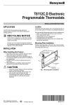
1
Control Systems Laboratory Collection Editors: Nick Lin Eduardo Gildin Robert Bishop Control Systems Laboratory Collection Editors: Nick Lin Eduardo Gildin Robert Bishop Authors: Robert Bishop Eduardo Gildin Nick Lin Erik Luther Online: < http://cnx.org/content/col10302/1.5/ > CONNEXIONS Rice University, Houston, Texas This selection and arrangement of content as a collection is copyrighted by Robert Bishop. It is licensed under the Creative Commons Attribution 2.0 license (http://creativecommons.org/licenses/by/2.0/). Collection structure revised: October 20, 2005 PDF generated: October 25, 2012 For copyright and attribution information for the modules contained in this collection, see p. 75. Table of Contents 1 Control Systems Lab Introduction, Hardware, Software, and Safety . . . . . . . . . . . . . . . . . . . . . . . . 1 2 Control Lab Setup: Choosing Control System Hardware and Software . . . . . . . . . . . . . . . . . . . . . 9 3 Control Lab Setup: Using LabVIEW to Control ECP Plants . . . . . . . . . . . . . . . . . . . . . . . . . . . . . . . 17 4 Introduction to Lab Hardware and LabVIEW Implementation . . . . . . . . . . . . . . . . . . . . . . . . . . . . . 25 5 System Identication for the Rectilinear Plant . . . . . . . . . . . . . . . . . . . . . . . . . . . . . . . . . . . . . . . . . . . . . . . 33 6 Rigid Body PD and PID Control . . . . . . . . . . . . . . . . . . . . . . . . . . . . . . . . . . . . . . . . . . . . . . . . . . . . . . . . . . . . . . . 39 7 Collocated / Noncollocated Control of 2DOF Rectilinear System . . . . . . . . . . . . . . . . . . . . . . . . . . 45 8 System Identication for the Torsional Plant . . . . . . . . . . . . . . . . . . . . . . . . . . . . . . . . . . . . . . . . . . . . . . . . . 51 9 Phase-Lead Compensation of a Rotational Rigid-Body System . . . . . . . . . . . . . . . . . . . . . . . . . . . . . 55 10 State Feedback Compensation of a 2DOF Rectilinear System . . . . . . . . . . . . . . . . . . . . . . . . . . . . . 59 11 Inverted Pendulum on a Translating Base . . . . . . . . . . . . . . . . . . . . . . . . . . . . . . . . . . . . . . . . . . . . . . . . . . . 63 12 Self-Erecting Inverted Pendulum on a Rotating Base . . . . . . . . . . . . . . . . . . . . . . . . . . . . . . . . . . . . . . . 69 Index . . . . . . . . . . . . . . . . . . . . . . . . . . . . . . . . . . . . . . . . . . . . . . . . . . . . . . . . . . . . . . . . . . . . . . . . . . . . . . . . . . . . . . . . . . . . . . . . 74 Attributions . . . . . . . . . . . . . . . . . . . . . . . . . . . . . . . . . . . . . . . . . . . . . . . . . . . . . . . . . . . . . . . . . . . . . . . . . . . . . . . . . . . . . . . . . 75 iv Available for free at Connexions <http://cnx.org/content/col10302/1.5> Chapter 1 Control Systems Lab Introduction, Hardware, Software, and Safety 1 1.1 Introduction 1.1.1 About this manual The purpose of this manual is to provide you, the student, with the laboratory procedures necessary for conducting the control system experiments in the ASE 170P course. You should by no means treat this manual as the sole source of information for the design and implementation process. You should rely on lecture notes, reference text, as well as their own knowledge of control theory, to develop and implement your control algorithms. This manual is only intended to provide an organized method for performing the experiments. 1.1.2 Course Objectives • To learn how to investigate the properties of physical systems both through simulation and experimentation. • • To learn how to perform hardware identication experiments on a physical plant. To learn how to design and analyze control systems through simulation using both classical and modern control techniques. • • • To learn how to simulate control systems using both state space and transfer function representations. To learn how to implement custom control algorithms in LabVIEW. To further develop skills for working with others in an experimental environment. 1.1.3 Course Policies Doing Your Own Work While you are encouraged to discuss theory and methods with other classmates, when it comes time to analyze, design, and implement your system, it must be done on your own. As an engineer you must always fully understand the problem you are trying to solve. Simply copying the work of others shows your lack of understanding of the problem. Remember, when you become an engineer working in industry, it is no longer just your grade that is at risk; your company's reputation, and more importantly other people's lives, are on the line. Any students caught in violation of these guidelines will be dealt with according to the university's policies on scholastic dishonesty. 1 This content is available online at <http://cnx.org/content/m13025/1.3/>. Available for free at Connexions <http://cnx.org/content/col10302/1.5> 1 CHAPTER 1. 2 CONTROL SYSTEMS LAB INTRODUCTION, HARDWARE, SOFTWARE, AND SAFETY Late Work Any work submitted late without a valid reason will not receive credit. If a student has a valid reason why an assignment must be submitted late, he/she should contact the instructor as soon as possible. Grading When working in an experimental environment, results are always important, but so is your ability to communicate the information with others. Any work you submit should be neat, well organized, and easy to understand. Remember, your work is a demonstration of your ability to understand the material you are studying as well as a reection of your organizational skills and attention to detail. The following guidelines will help ensure that you receive as much credit as possible for your work: 1. Your derivation of the system's dynamic equations should be neat, easy to follow, and mathematically correct. In addition, remember to always draw a free-body diagram and label any system parameters and variables that will appear in your derivation. 2. The process you use to design your controller should be well outlined. In other words, don't just hand in your nal design; show the steps you took to arrive at that design. 3. Any LabVIEW VI that you write should be well organized and easy to follow (e.g. avoid crossing wires whenever possible). Remember, the diagram code should follow well from left to right. Furthermore, a neat and well organized VI will make the debugging process easier for you should problems arise. 4. When performing experiments in the lab, always record any important data that is acquired from the system; they may be necessary for calculations that you will need to perform later. 5. Your answers to the post-lab questions should demonstrate that you fully understand all aspects of the experiment(s) you just performed. Also, remember that with experimentation there is often no "right" answer. You should answer the question based on your observations and the results obtained from your particular system, which may be very dierent than somebody else's. Program Debugging Some students tend to think of the instructor as a program debugging aid. to nd your own errors before seeking assistance. You should try diligently Part of the objective of the computer assignments is to help you develop the ability to use the computer INDEPENDENTLY. You are not using the computer independently if someone else debugs your programs. You should only seek debugging assistance from the instructor if you have made a diligent eort to nd your mistakes. Available for free at Connexions <http://cnx.org/content/col10302/1.5> 3 1.2 Lab Hardware The experiments for this course will be performed on plants from ECP (Educational Control Products), which will be controlled by a National Instruments PXI chassis equipped with an embedded real-time controller and a recongurable multifunction I/O module. 1.2.1 Model 210 Rectilinear Plant 2 holds three mass carriages which can be loaded with brass weights The ECP Model 210 Rectilinear Plant and connected in a variety of congurations using springs of varying stiness. The adjustable dashpot can be used to provide damping for the system. A single drive motor provides actuation to the system via the rst mass carriage, and position measurements are taken by quadrature encoders. ECP Model 210 External Image Please see: http://www.ecpsystems.com/subPageImages/lin.gif Figure 1.1: ECP Model 210 Rectilinear Plant3 1.2.2 Model 205 Torsional Plant 4 holds three disks each of which can be loaded with brass weights at The ECP Model 205 Torsional Plant varying positions. The disks are connected through their centers by thin rods giving the system rotational stiness. A single driver motor actuates the system via the bottom disk, and quadrature encoders provide angular position measurements. ECP Model 205 External Image Please see: http://www.ecpsystems.com/subPageImages/tors.gif Figure 1.2: ECP Model 205 Torsional Plant5 2 http://www.ecpsystems.com/controls_torplant.htm 3 http://www.ecpsystems.com/controls_torplant.htm 4 http://www.ecpsystems.com/controls_recplant.htm 5 http://www.ecpsystems.com/controls_recplant.htm Available for free at Connexions <http://cnx.org/content/col10302/1.5> CHAPTER 1. 4 CONTROL SYSTEMS LAB INTRODUCTION, HARDWARE, SOFTWARE, AND SAFETY 1.2.3 A-51 Inverted Pendulum Accessory The ECP A-51 Inverted Pendulum Accessory 6 consists of a cylindrical weight attached to a slender rod. The position of the weight can be varied therefore changing the center of gravity of the assembly. The rod attaches to a low friction pivot joint whose angular position is measured by a quadrature encoder. The base plate allows for the accessory to be mounted on both the Model 210 and Model 205 plants. ECP A-51 External Image Please see: http://www.ecpsystems.com/subPageImages/penasscMain.gif Figure 1.3: ECP A-51 Inverted Pendulum Accessory7 1.2.4 PXI-1042 Chassis The National Instruments PXI-1031 chassis 8 provides a foundation to which a variety of PXI expansion modules can be added. This makes it a highly customizable measurement and testing platform. 6 http://www.ecpsystems.com/controls_pendassc.htm 7 http://www.ecpsystems.com/controls_pendassc.htm 8 http://sine.ni.com/nips/cds/view/p/lang/en/nid/13906 Available for free at Connexions <http://cnx.org/content/col10302/1.5> 5 NI PXI-1031 Figure 1.4: National Instruments PXI-1031 Chassis9 1.2.5 PXI-8186 Real-Time Embedded Controller 10 is a Pentium4-based, real-time embedded controller. In addition to The National Instruments PXI-8186 having the ability to act as a Windows PC, the PXI-8186 can also run an NI developed, real-time operating system which allows it to work as a deployment platform for LabVIEW Real-Time applications. 9 http://sine.ni.com/nips/cds/view/p/lang/en/nid/13906 10 http://sine.ni.com/nips/cds/view/p/lang/en/nid/13447 Available for free at Connexions <http://cnx.org/content/col10302/1.5> CHAPTER 1. 6 CONTROL SYSTEMS LAB INTRODUCTION, HARDWARE, SOFTWARE, AND SAFETY NI PXI-8186 Figure 1.5: National Instruments PXI-8186 Embedded Controller11 1.2.6 PXI-7831R Recongurable Multifunction I/O The National Instruments PXI-7831R Recongurable Multifunction I/O 12 is a module that can input and output both analog and digital signals. It is equipped with an FPGA (eld processor gate array) which is congurable with the LabVIEW FPGA Module. 11 http://sine.ni.com/nips/cds/view/p/lang/en/nid/13447 12 http://sine.ni.com/nips/cds/view/p/lang/en/nid/14757 Available for free at Connexions <http://cnx.org/content/col10302/1.5> 7 NI PXI-7831R Figure 1.6: National Instruments PXI-7831R Recongurable Multifunction I/O13 1.3 Safety Procedures The following procedures are to help prevent damage to the lab equipment and also to ensure your safety. Be sure to read and understand all of the information in this section before performing any experiments. Should you ever have any questions regarding the operation of the lab hardware, do not hesitate to ask the instructor. 1.3.1 General Safety Precautions • Always check to make sure that all of the system components (brass weights, disks, spring, etc) are securely fastened before powering on the ECP amplier box and implementing your VI. • Whenever you are reconguring the plant setup, always be sure to check that your VI is not running and that the amplier box is turned o. • When implementing an untested control algorithm, check for stability by using a long slender object (such as a ruler or unsharpened pencil) to apply gentle force to the mass/disk nearest to the drive 13 http://sine.ni.com/nips/cds/view/p/lang/en/nid/14757 Available for free at Connexions <http://cnx.org/content/col10302/1.5> CHAPTER 1. 8 CONTROL SYSTEMS LAB INTRODUCTION, HARDWARE, SOFTWARE, AND SAFETY motor. • • Do not disturb the system while it is executing a commanded trajectory. In the event of an emergency, shut o power to the system by pressing the red button on the amplier box. 1.3.2 Hardware Limits on the Model 210 Located near each mass carriage are two stop bumpers that prevent the carriage from exceeding their maximum allowable displacement. when it is engaged. On each stop bumper is an electrical switch which sends out a signal When the LabVIEW FPGA code receives this signal, it immediately outputs zero command voltage to the drive motor. This voltage remains zero until the error is cleared via the control loop VI's front panel. In addition to the limit switches, the FPGA code has been written to prevent overspeed / overvoltage of the drive motor. When the code detects overspeeding / overvolting of the motor, it will again output zero command voltage and remain there until the error has been cleared. 1.3.3 Hardware Limits on the Model 205 The FPGA code for the model 205 plant has been written to detect when the relative position between the rst and second disks exceeds 3000 counts. torque is applied to the base disk. This is to prevent damage to the torsional rod if a large When this limit is exceeded, zero command voltage is output to the drive motor until the error is cleared. Just as with the model 210 plant, the model 205 also has drive motor over-speed/overvoltage protection incorporated into the FPGA code. Available for free at Connexions <http://cnx.org/content/col10302/1.5> Chapter 2 Control Lab Setup: Choosing Control System Hardware and Software 1 1 This content is available online at <http://cnx.org/content/m13071/1.9/>. Available for free at Connexions <http://cnx.org/content/col10302/1.5> 9 CHAPTER 2. 10 CONTROL LAB SETUP: CHOOSING CONTROL SYSTEM HARDWARE AND SOFTWARE 2.1 Choosing Lab Equipment 2.1.1 Software 2.1.1.1 National Instruments Applications and Toolkits • • • • • LabVIEW 7.1, 8.0, or 8.2 Full Development System LabVIEW Real Time ETS or RTX (more detail under Choosing Lab Hardware) LabVIEW Control Design Toolkit LabVIEW Simulation Module LabVIEW FPGA 2.1.1.2 National Instruments Drivers: • • LabVIEW Device Driver CDs NI-RIO Driver CD 2.1.1.3 Venturecom Applications • Real Time eXtention for Windows (RTX) (Optional) Available for free at Connexions <http://cnx.org/content/col10302/1.5> 11 2.1.2 Choosing Lab Hardware The lab currently uses the hardware laid out as option one (1) below, LabVIEW Real-Time Module for ETS with PXI hardware. However, there are several hardware combinations that can be used for implementation of a Real-Time system to control ETS plants using LabVIEW. These options each have their own benets. The options have been broken down by Real Time OS software support. Available for free at Connexions <http://cnx.org/content/col10302/1.5> CHAPTER 2. 12 CONTROL LAB SETUP: CHOOSING CONTROL SYSTEM HARDWARE AND SOFTWARE 2.1.2.1 LabVIEW Real-Time Module for ETS The LabVIEW Real-Time Module for ETS targets is for real-time devices that use a single dedicated kernel running embedded code. This option can be purchased from National Instruments for real-time PXI targets. It is also used for desktop PCs running as a dedicated real-time target. Figure 2.1: LabVIEW Real Time for ETS Options 1. This option consists of a Windows PC communicating with a PXI real-time controller running LabVIEW Real-Time OS. The PXI-7831R intelligent data acquisition board is connected to the controller through the PXI bus. Control loops can be executed on both the Real-Time controller and on the intelligent data acquisition board. The ECP-RIO Adapter cable 2 connects the 68pin VHDCI connector from the MIO connector on the PXI-7831R to the round encoder cable connected directly to the ECP plant. The banana plugs connect to the motor drive inputs on the front of the ECP Power supply. The ECP Amplier is then connected to one of ECP's mechanical plants. PXI provides a portable computing and acquisition solution that is rugged and rated for enviormnets where normal PC's can't go, making it ideal for both laboratory and research applications in many types of environments where determinism and reliability are crucial. PXI Control System (ETS) :: PXI Advisor for conguring a PXI system from National Instruments 3 2. This option consists of a Windows PC communicating with a second PC running LabVIEW Real-Time OS (Real-Time OS PC Requirements) the PC through the PCI bus. 4 . The PCI-7831R intelligent data acquisition board is connected to Control loops can be executed on both the Real-Time OS running on the PCI and in the RIO intelligent data acquisition board. The ECP-RIO Adapter cable 5 connects the 68pin VHDCI connector from the MIO connector on the PXI-7831R to the round encoder cable connected directly to the ECP plant. The banana plugs connect to the motor drive inputs on the front of the ECP Power supply. The ECP Amplier is then connected to one of ECP's mechanical plants. 2 http://cnx.org/content/m13071/latest/ECP-RIO_Adapter.pdf 3 http://ohm.ni.com/advisors/pxi 4 http://digital.ni.com/public.nsf/websearch/CB3434DA94466DD286256E9E006BB775 5 http://cnx.org/content/m13071/latest/ECP-RIO_Adapter.pdf Available for free at Connexions <http://cnx.org/content/col10302/1.5> 13 The Real-Time PC solution provides a lower cost real-time computing and acquisition platform that is ideal for laboratory and research applications, while still maintaining determinism and reliability. 6 Real-Time PC (ETS) :: Real-Time Control System Bundle for Academia from National Instrumets 6 http://digital.ni.com/express.nsf/bycode/exxu63 Available for free at Connexions <http://cnx.org/content/col10302/1.5> CHAPTER 2. 14 CONTROL LAB SETUP: CHOOSING CONTROL SYSTEM HARDWARE AND SOFTWARE 2.1.2.2 The LabVIEW Real-Time Module for RTX The LabVIEW Real-Time Module for RTX targets is used with desktop PCs running RTX, a real-time extension for Windows. This real-time operating system runs in parallel with Windows on the same processor, providing a single box solution for both user interface and deterministic operations. The OS can be purchased from National Instruments or from Venturecom directly. LabVIEW for RTX is a single PC solution for Real Time processing. Figure 2.2: 3. LabVIEW Real Time for RTX Options This option consists of a Windows PC running Microsoft Windows, and Aredence's Realtime Ex- tensions (RTX) (Will my PC work with RTX? 7 ) Windows and RTX run on the same computer, sharing the same CPU, but applications run in RTX maintain real-time execution. The PCI-7831R intelligent data acquisition board communicates with the PC through the standard PCI bus. Control loops can be executed on both in RTX and on the intelligent data acquisition board. The ECP-RIO Adapter cable 8 connects the 68pin VHDCI connector from the MIO connector on the PXI-7831R to the round encoder cable connected directly to the ECP plant. The banana plugs connect to the motor drive inputs on the front of the ECP Power supply. The ECP Amplier is then connected to one of ECP's mechanical plants. The Real-Time RTX solution provides a single PC, low cost real-time computing and acquisition platform that is acceptable for laboratory applications. Single PC (RTX) :: Real-Time Control System Software and Hardware Bundle for Academia from National Instruments 9 7 http://digital.ni.com/public.nsf/allkb/03BC0810E60CE93286256E7D007B61F5 8 http://cnx.org/content/m13071/latest/ECP-RIO_Adapter.pdf 9 http://digital.ni.com/express.nsf/bycode/exxu63 Available for free at Connexions <http://cnx.org/content/col10302/1.5> 15 2.1.2.3 Intellegent Data Acquision I/O Board :: PCI/PXI-7831R Recongurable Multifunction I/O Using the LabVIEW FPGA Module Each solution uses the National Instruments PCI-7831R Recongurable FPGA. The FPGA is most useful because it oers 8 analog inputs, 8 analog outputs, and 96 digital I/O lines making it scalable for both teaching applications and research. The on board FPGA can be given a xed personality for student use, or can be reprogrammed with the LabVIEW FPGA Module specically for your needs. PID control loop rates up to 200,000 Hz. The 7831R also allows custom safety features to be implemented in the FPGA to protect students and equipment. Because these safety features are implemented in hardware, they are not dependent on the stability of the code running on the PC or real-time OS. User's Manual for the PCI-7831R and PXI-7831R 10 The following instructions and pin outs detail the wiring between the NI 7831R FPGA board to the ECP amplier box. This cable is built and sold by National Instruments. You can download the cable detail and 11 pin outs here: ECP Plant to NI RIO FPGA board (Download) 2.1.2.4 ECP Hardware Please see ECP's website for more information on ECP hardware options. ECP Systems Website 12 10 http://www.ni.com/pdf/manuals/370489b.pdf 11 http://cnx.org/content/m13071/latest/ECP-RIO_Adapter.pdf 12 http://www.ecpsystems.com/controls_family.htm Available for free at Connexions <http://cnx.org/content/col10302/1.5> 16 CHAPTER 2. CONTROL LAB SETUP: CHOOSING CONTROL SYSTEM HARDWARE AND SOFTWARE 2.2 Lab Setup 2.2.1 Software Installation 13 Step-by-step control system software installation instructions (Download) 13 http://cnx.org/content/m13071/latest/Software_Installation_Notes.doc Available for free at Connexions <http://cnx.org/content/col10302/1.5> Chapter 3 Control Lab Setup: Using LabVIEW to Control ECP Plants 1 1 This content is available online at <http://cnx.org/content/m13080/1.4/>. Available for free at Connexions <http://cnx.org/content/col10302/1.5> 17 CHAPTER 3. 18 CONTROL LAB SETUP: USING LABVIEW TO CONTROL ECP PLANTS 3.1 Using LabVIEW to Control ECP Plants This document provides a brief overview of how to use the National Instruments LabVIEW Virtual Instrument (VI) developed by The University of Texas at Austin Aerospace Engineering Controls Laboratory to perform control system experiments with the Educational Control Products (ECP) Model 210 Rectilinear and Model 205 Torsional plants. 3.1.1 FPGA Personality VIs: 3.1.1.1 FPGA VI Specics for each Plant The provided FPGA VIs contain the code for the recongurable I/O board which sends and receives signals, such as motor drive voltage and quadrature encoder channels, from the plants. Furthermore, the FPGA code incorporates safety features, such as motor overvoltage protection, to help prevent damage to the plants. The FPGA VIs for the two plants are similar but dier in the following ways: 1. For the Model 205 Torsional Plant, the A and B channels for encoder 3 have been switched due to the fact that the physical orientation of encoder 3 is opposite that of encoders 1 and 2. 2. The Model 205 Torsional Plant does not have limit switches, but to prevent damage to the torsion rods, the VI will write zero voltage to the drive motor in the event that the displacement between disks 1 and 2 or disks 2 and 3 exceeds 3000 counts (67.5 degrees). The voltage will remain at zero until the error is cleared. • File Name of LabVIEW 8.0 Project: ECP 205 Project.lvproj (within LabVIEW 8.0 Starting Point.zip below) • File Name of LabVIEW 7.1 Project: ECP 205.lep (within LabVIEW 7.1 Starting Point.zip below) 3. The Model 210 Rectilinear Plant has limit switches to prevent damage due to excessive travel of the mass carriages. If a limit switch is engaged, the VI returns a value of true to an error indicator and writes zero voltage to the drive motor until the error is cleared. • File Name of LabVIEW 8.0 Project: ECP 210 Project.lvproj (within LabVIEW 8.0 Starting Point.zip below) • File Name of LabVIEW 7.1 Project: ECP 210.lep (within LabVIEW 7.1 Starting Point.zip below) note: The FPGA personality can be dowloaded with example programs below under Starting- Point VI's for Each Plant (Section 3.1.2.1: Starting-Point VI's for Each Plant). The FPGA VI for both plants incorporates drive motor overvoltage protection. If an overvoltage condition is detected, zero voltage will be written to the motor until the error is cleared. The portion of the code which interprets encoder signals has been written such that for the 210 plant, a displacement to the right results in a positive measurement. For the 205 plant, a positive measurement results from a counterclockwise disk displacement. When using the ECP pendulum accessory, a counterclockwise rotation will result in a positive encoder measurement (encoder 4). The portion of the code which sends signals to the drive motor has been written such that a positive control eort results in a counterclockwise (when viewed from the shaft) rotation of the drive motor. Therefore, for the 210 plant, this will result in an input force to the right. For the 205 plant, this will result in a clockwise input torque at the base disk. If you decide to write new FPGA code using the LabVIEW Embedded Project Manager, use the following tables as a reference for assigning FPGA channels: • Note that if you use the ECP pendulum accessory and are required to connect the pendulum encoder cable manually to the terminal block inside the amplier box, then you should connect the +5V and ground wire to pins 2 and 4, respectively, on the terminal block. This is due to the fact that the National Instruments ECP to RIO cable maps the +5V and ground channels for all the encoders to Available for free at Connexions <http://cnx.org/content/col10302/1.5> 19 only pins 2 and 4 on the terminal block. ECP may instruct you to connect the +5V and ground wires for encoder 4 to pins 1 and 3 on the terminal block; however, doing so will result in the encoder not receiving power. • Encoder Counts Per Revolution · · · · Encoder 1: 16000 counts = 360 degrees Encoder 2: 16000 counts = 360 degrees Encoder 3: 16000 counts = 360 degrees Encoder 4: 16384 counts = 360 degrees (pendulum encoder) ** note: See special hook-up instructions (p. 18) for the pendulum encoder on note above. This only applies to the ECP pendulum attachment that requires bare wires to be hooked up inside the ECP Amplier box. 3.1.1.2 Autorunning FPGA VIs to Zero Analog Outputs: note: This must only be done once for the life of the FPGA Board. To ensure that the system has the correct power on states when the real-time target is booted but before the control loop VI is run, you should congure the target to autorun the FPGA VI at power on. To enable this feature, the Autorun VI option should be selected when building the FPGA project code. Then, in the LabVIEW Embedded Project Manager, select Tools Download VI or Attributes to Flash Memory. In this window, you can download the FPGA VI from the host machine to the ash memory on the target and congure autoload options. See Chapter 4 of the LabVIEW FPGA Module User's Manual for more information. 3.1.2 Using the Real-Time VI for Control System Experiments 3.1.2.1 Starting-Point VI's for Each Plant • LabVIEW Real Time for ETS Example VIs · ECP 205 and 210 LabVIEW 8.0 Project: ECP_LabVIEW_8.0_Starting_Point.zip (download) - FPGA personality included · ECP 205 and 210 LabVIEW 7.1 Project: ECP_LabVIEW_7.1_Starting_Point.zip (download) 2 3 - FPGA personality included • LabVIEW Real Time for RTX Example VIs · · ECP 210 Rectilinear Plant: not yet posted ECP 205 Torsional Plant: not yet posted 3.1.2.2 Usage Instructions Extract all folders and VIs to a directory on your host PC. Be sure to keep the le and folder paths intact to avoid having to relocate VIs. The les in the FPGA VIs and Sub VIs folders do not need to be changed. Target your real-time device from the LabVIEW start-up screen and then open the example ECP 210 1DOF PID.vi. You will see the front panel shown below: 2 http://cnx.org/content/m13080/latest/ECP_LabVIEW_8.0_Starting_Point.zip 3 http://cnx.org/content/m13080/latest/ECP_LabVIEW_7.1_Starting_Point.zip Available for free at Connexions <http://cnx.org/content/col10302/1.5> CHAPTER 3. 20 CONTROL LAB SETUP: USING LABVIEW TO CONTROL ECP PLANTS LabVIEW front panel of example ECP 210 1DOF PID.vi (Section 3.1.2.1: Starting-Point VI's for Each Plant) Figure 3.1: Take a few moments to familiarize yourself with the various controls and indicators that are available on the front panel. When you are ready, power on the ECP amplier box and run the VI. Once the VI completes downloading to the PXI, the closed-loop system is active (or open-loop in the case of no controller). In this example, a PID controller is being used to control the position of a 1DOF rigid-body system. The rst mass cart on the ECP Model 210 plant is loaded with four 0.5kg weights and no springs or dashpots are attached. Available for free at Connexions <http://cnx.org/content/col10302/1.5> 21 Figure 3.2: Partial shot of the ECP Model 210 Plant You may apply a light external force to the mass cart and feel the controller respond by attempting to attenuate the disturbance. Also, notice that encoder position measurements are displayed on the front panel. Pressing the Reset Encoders control will set all the encoders back to 0. If any of the error conditions are detected (limit switches, drive motor overvoltage, etc), the VI will perform a safety shutdown and you will need to re-run it. If you wish to command a test signal to the system, press the Command Trajectory control. The Sub VI front panel shown below will pop open: Available for free at Connexions <http://cnx.org/content/col10302/1.5> CHAPTER 3. 22 CONTROL LAB SETUP: USING LABVIEW TO CONTROL ECP PLANTS Figure 3.3: note: The Command tragjectory interface Test Signals feature is only available when using LabVIEW Real-Time for ETS, because of the additional overhead required for the interactive user interface. Take a moment to tab through the various types of test signals that are available as well as what parameters you may prescribe for each signal. Selecting the bidirectional inputs option causes the commanded signal to alternate directions when more than one repetition is specied. Trajectory control to see a preview of the signal. You may always press the Preview When you are satised with your selection, press the Execute Trajectory control. The Sub VIs front panel will close and the signal will be sent to the system as the reference trajectory that is to be tracked. When the trajectory is complete, plot data will be calculated. This may take a few seconds depending on the duration of your specied trajectory. When the data calculation completes you may toggle on and o any trajectories that you wish to view on the graph indicator such as position, velocity, and acceleration. Note that the velocity and acceleration amplitudes have been scaled by 0.1 and 0.01, respectively, on the graph. Try using the graph indicator's zoom options if you wish to zoom in on a portion of the graph. Toggling the cursor on brings up the cursor on the graph. You may lock the cursor to any of the 14 plot histories and click and drag on it to obtain point-by-point numeric data. The rst number shown in the cursor legend is the time and the second is the amplitude for the plot to which you are currently locked. If you wish to save the data, enter a le name in the path control on the front panel and press the Save Raw Data control. This will save the time, reference signal, control eort, and four encoder position histories for the commanded trajectory; velocity and acceleration data are not saved. The le is saved as spreadsheet data on the PXI's hard drive. You may use an FTP client of your choice to access the PXI and copy the le Available for free at Connexions <http://cnx.org/content/col10302/1.5> 23 to your host machine. When you are nished with your experiment, press the Abort Control control on the front panel and the VI will shut down the control loop. Programming a Control Algorithm in the VI's Block Diagram: The Real-Time control loop VI has been written such that a variety of control algorithms can be imple- mented with little change to the VI's block diagram code. The only change that needs to be made is the code that exists between the reference signal (desired position) and the control eort (analog output). Open the block diagram for the VI (shown below) to see how the PID controller for this example was implemented: Partial block diagram view of Example VI ECP 210 1DOF PID.vi (Section 3.1.2.1: StartingPoint VI's for Each Plant) Figure 3.4: The encoder measurement is subtracted from the reference signal to generate the error signal, which is sent through the PID algorithm. Finally, the control eort signal calculated by the PID is sent to the analog output channel that drives the plant motor. It can be seen that programming other controllers such as phase lead, LQR, etc could be easily accomplished by deleting the current algorithm and coding a new one in its place. To perform experiments for the open-loop case (useful when studying the system's natural dynamics or when performing system identication), you may simply delete the feedback control algorithm and connect the reference trajectory point directly to the analog output. Recall that the analog output channels on the recongurable I/O board have a range of +10V to -10V and a 16-bit DAC resolution. Available for free at Connexions <http://cnx.org/content/col10302/1.5> Therefore, in the CHAPTER 3. 24 CONTROL LAB SETUP: USING LABVIEW TO CONTROL ECP PLANTS open-loop case, a command signal amplitude of -32768 to +32767 corresponds to -10V to +10V sent to the drive motor. Please refer to the following resources for more detailed plant dynamics and hardware descriptions: ECP Plant Manuals and National Instruments Resources: • • • • Manual for Model 210/210a Rectilinear Control System (Instructor's Edition) Manual for Model 205/205a Torsional Control System (Instructor's Edition) National Instruments PCI/PXI 7831R Hardware: http://www.ni.com/pdf/manuals/370489b.pdf 4 Additional NI hardware and LabVIEW programming resources can be found on http://www.ni.com/ 4 http://www.ni.com/pdf/manuals/370489b.pdf 5 http://www.ni.com/ Available for free at Connexions <http://cnx.org/content/col10302/1.5> 5 Chapter 4 Introduction to Lab Hardware and LabVIEW Implementation 1 1 This content is available online at <http://cnx.org/content/m13026/1.3/>. Available for free at Connexions <http://cnx.org/content/col10302/1.5> 25 CHAPTER 4. 26 INTRODUCTION TO LAB HARDWARE AND LABVIEW IMPLEMENTATION 4.1 Introduction to Lab Hardware and LabVIEW Implementation 4.1.1 Objectives • • • Become familiar with how the lab hardware works Understand how the LabVIEW control loop block diagram executes Gain experience in interacting with the VI front panel Available for free at Connexions <http://cnx.org/content/col10302/1.5> 27 4.1.2 Pre-Lab 1. In your own words, describe how the implementation VI's block diagram executes. More specically, explain the execution when the system is idle and when a reference trajectory is commanded. Available for free at Connexions <http://cnx.org/content/col10302/1.5> CHAPTER 4. 28 INTRODUCTION TO LAB HARDWARE AND LABVIEW IMPLEMENTATION 4.1.3 Lab Procedure 4.1.3.1 Using the Model 210 Rectilinear Plant 1. Connect the drive motor and encoder feedback cables to the Model 210 plant. 2. Unclamp the rst mass carriage and remove any springs that may be connected to it. Be sure to position the stop bumpers to allow maximum range of motion for the carriage. Load four 0:5kg brass weights onto the carriage. In this conguration the carriage acts as a rigid-body system. 3. Clamp the other two mass carriages by moving the stop bumpers inward so they constrain the motion of the carriage. You will need to use a 1/4 inch spacer nut between the mass carriage and stop bumpers so as to not engage the limit switches. 4. Power on the PXI by pressing the rectangular button located at the bottom left corner of its front face. Wait approximately 30 seconds for the system to boot up. 5. Run LabVIEW on your host PC. 6. Target the PXI real-time embedded controller by selecting RT Target: 146.6.105.x note: (the IP address of your PXI system) from the Execution Target drop-down menu on the LabVIEW startup screen. Wait for LabVIEW to establish a connection. 7. Now click the Open button on the LabVIEW startup screen and locate the le named Lab 1 - Intro to Lab Hardware.vi. The VI front panel should look like the one in Fig. 1. Available for free at Connexions <http://cnx.org/content/col10302/1.5> 29 LabVIEW Figure 4.1: VI Front Panel 1. Enter a loop time of 0.005 seconds then run the VI by clicking on the arrow button at the top-left corner of the front panel (because of the way that the VI's block diagram is written, you must enter the loop time before running the VI. If you wish to change the loop time, you must stop the VI, enter the new loop time, and then run the VI again). At this time, the VI code will be downloaded from the host PC to the PXI. When downloading is complete, the VI will automatically begin executing on the RT system. At this time, the control loop is being run solely on the PXI's real-time embedded controller, not your host PC. However, a communications loop is running between the two systems to allow the user to interact with front panel activities. note: The communications loop is part of the LabVIEW Real-Time Development system. You do not see its code anywhere in the VI 2. Manually displace the rst mass carriage and observe the position measure- ment being shown by the Encoder 1 indicator on the front panel. Notice that even when the amplier box is powered o, the encoders still make measurements. The Encoder 2 and Encoder 3 indicators correspond to the second and third mass carriages, respectively. The Encoder 4 indicator is for the pendulum accessory and will be used later in the course. Available for free at Connexions <http://cnx.org/content/col10302/1.5> CHAPTER 4. 30 INTRODUCTION TO LAB HARDWARE AND LABVIEW IMPLEMENTATION 3. Whenever you wish to set the encoder readings to zero, simply press the Reset Encoders control located on the front panel. Try this now. 4. Now manually displace the rst mass carriage until you engage one of the limit switches. Notice how the System Error indicator lights up. At this point, if any voltage were being output to the drive motor, it would be set to zero and remain there until you press the Clear Error control on the front panel. Press this control now and observe how the System Error indicator light turns o. 5. You are now going to send a commanded trajectory to the plant. First, power on the amplier box by pressing the black button. Also, center the rst mass carriage between the two stop bumpers and then reset the encoders. 6. Now press the Command Trajectory control on the front panel. The front panel for the Test Signals.vi subVI will pop open. Click through the dierent types of test signals you can command the system with, and notice the dierent parameters that you can change for each signal. Choose one of the signals and enter values for its parameters. Then click on the Preview Trajectory control and observe the signal on the graph indicator. Notice the eect of selecting the Bidirectional Inputs control on signals for which you specify more than one repetition. 7. Choose a sinusoidal signal with an amplitude of 1640 counts. This amplitude corresponds to an input of 0.5 Volts to the drive motor and 2.6 Newtons to the mass carriage, nominally. You will learn how to calculate these exact values in the next lab. Set the frequency to 2Hz, and repeat the signal 8 times. Preview the trajectory to check that it is what you expected (it is always good practice to preview the test signal before you execute it to make sure you know exactly what will be commanded). 8. Once you have conrmed that the commanded trajectory is correct, press the Execute Trajectory control. The Test Signals.vi front panel will close and the Executing Trajectory indicator on the main VI's front panel will light up. During this time you will see the plant responding to the command. When the trajectory is complete, the plot data will be computed, as shown by the Computing Plot Data indicator. Once complete, you may choose which trajectories you wish to view by selecting the corresponding check box. If necessary, use the zoom features for the graph indicator to get a better view of the data. Also, select the cursor tool and drag the cursor over the response plot. 9. Notice that time and amplitude data is shown in the cursor legend. This feature will become useful for performing calculations in later labs. Take a look at the response of the rst mass carriage which you just commanded. Since no control algorithm was implemented, you are looking at the open-loop response of the system. 10. If you wish to save the data to a spreadsheet le, enter a lename in the le path box and press the Save Raw Data control. Note that this only saves the time, reference trajectory, control eort, and encoder data, not the velocity or acceleration. The le will be saved to the hard drive on the PXI. You can use an FTP client to download the le to your host PC. The le can be imported by any application that can handle spreadsheets such as Excel or Matlab. 11. Also, you can save the response plot for later viewing or inserting into a report. The easiest way to do this is to simply right click on the plot and choose the Copy Data option (this option will be under the Data Operations menu if the VI is not running). Then just paste the gure into an image editing program (such as Paint) or a word processing application that can handle embedded images. Unchecking the Autoscale Y Axis option will help ensure that the pasted image will look the same as it does on the VI front panel. Save the plot of the reference trajectory and response of the rst mass carriage that you just commanded and hand it in with the rest of your work. 12. You are now nished with the introduction to using LabVIEW with the Model 210 plant. Press the Abort Control button on the front panel and turn o the amplier. At this time take a few minutes to connect the springs and dashpot to the mass carriages so you will be familiar with this process in future labs. The springs are available in three stinesses that you will determine in the next lab. The damping provided by the dashpot can be varied by turning the knob located at the end. Turning it counterclockwise decreases the damping while turning it clockwise increases the damping. For a given dashpot setting, you can determine the damping coecient experimentally, as you will see in the next lab. Available for free at Connexions <http://cnx.org/content/col10302/1.5> 31 13. When you are nished turn o the amplier box. 4.3.2 Using the Model 205 Torsional Plant 14. Connect the drive motor and encoder feedback cables to the Model 205 plant. 15. Mount disks to all three locations. When mounting a disk at the uppermost location, always be sure that you mount the disk on the underside of the center mounting hub. The bottom and middle disks should be mounted on top of the mounting hub. You should mount the disks so that the side with the concentric circles is facing up. 16. Load two 0:5kg brass weights onto the second disk so they both lie on the diameter line of the disk (i.e. 180o apart). Place the center of each weight 9:0cm from the center of the disk. You can determine this by looking at the concentric circles that have been cut into the disks. The inner most circle is 2:0cm from the center, and each successive circle occurs at 1:0cm intervals. note: Whenever mounting weights onto the disks, the threaded locking nut needs to be positioned so that it falls into the groove on the underside of the disk. This helps prevent the weights from jittering around on the disk. The same should be done when clamping the disks as well. 17. Now clamp the upper disk so that it cannot rotate. 18. Take a look at the VI's block diagram. At the far left you will notice that the FPGA code we are referencing is that of the Model 210 (the reference is being established by the pink icon that says ECP 210 on it). However, the FPGA codes of the Model 210 and Model 205 are slightly dierent, so we wish to change this reference to that of the Model 205. Right click on the icon and choose Select Target VI. Then locate and select the ECP Timed (FPGA) sync 205.vi le. Once LabVIEW has established the reference, you will see the text on the icon change from ECP 210 to ECP 205. As a nal step, right click the icon again and choose Refresh. 19. Now save the VI by using the File drop-down menu (or alternately by pressing Ctrl + S on your keyboard). Then run the VI. 20. Manually displace the rst and second disks and observe the encoder measurements on the front panel. Notice that the encoders make positive measurements in the counterclockwise direction (with respect to a top view reference position). You will need to remember this for the future when you derive the torsional plant's equations of motion. When you are nished, reset the encoders. 21. Now turn on the amplier box. 22. Suppose we wish to acquire and view the natural response of the system for a particular set of initial conditions. You can accomplish this by executing a step with zero amplitude (hence zero control eort is being input to the plant). Select a dwell time of 4000ms. This will cause the system to acquire 8 seconds of data. To see why this is true, preview a step input with a nonzero amplitude and observe how the dwell time is dened for this type of input. 23. Now execute the zero amplitude step and manually displace the rst disk by approximately 45o, then release it. Wait for the VI to nish acquiring the data, and then plot the measurements from encoder 1 and 2. Try a dierent set of initial conditions (e.g. displace the two disks in opposing directions) and observe the response. 24. Reset the encoders and execute a sine sweep with a 500 count amplitude (again, you will learn how to compute the drive motor voltage and torque corresponding to this amplitude in the next lab). Enter 0:1Hz and 10Hz as your start and end frequencies, respectively. Input a sweep time of 30 seconds and set the sweep method to logarithmic. When the sweep is complete, select to view the frequency response from the control on the front panel. This is a 2DOF spring, mass, damper system. Does the response look familiar? Save the plot of the disk 1 and 2 frequency responses and hand it in with the rest of your work. 25. You are now nished with you introduction to the Model 205 plant. Stop the VI by hitting the Abort Control button and turn o the amplier box. 26. Close all VI windows and exit LabVIEW. Then turn o the PXI. 27. Return all plant materials to the instructor. Available for free at Connexions <http://cnx.org/content/col10302/1.5> CHAPTER 4. 32 INTRODUCTION TO LAB HARDWARE AND LABVIEW IMPLEMENTATION 4.1.4 Post-Lab 1. Consider a controller Gc(s) in series with a plant G(s) with unity negative feedback. Denote the reference input, tracking error, control eort, and output by R(s), E(s), U(s), and Y (s), respectively. Draw the block diagram for this system making sure to label all the signals. 2. Now consider the hardware we have in the lab. Instead of having just Gc(s), G(s), etc, draw a diagram that shows each piece of lab hardware and which signal(s) it sends and/or receives. should include at least the following: • • • • • • mass carriages or torsion disks (choose either one) amplier box PXI Recongurable I/O module Encoders drive motor PXI embedded controller 3. Be sure to label all forces/torques, displacements, and signals that occur in the system. Available for free at Connexions <http://cnx.org/content/col10302/1.5> Your diagram Chapter 5 System Identication for the Rectilinear Plant 1 5.1 System Identication for the Rectilinear Plant 5.1.1 Objectives • • • Review of the behavior of second-order systems Understand the importance of system identication Understand the concept of hardware gain and why it will play a crucial role in controller design 1 This content is available online at <http://cnx.org/content/m13066/1.1/>. Available for free at Connexions <http://cnx.org/content/col10302/1.5> 33 34 CHAPTER 5. SYSTEM IDENTIFICATION FOR THE RECTILINEAR PLANT 5.1.2 Pre-Lab 1. Derive the equations of motion for the 1DOF spring-mass system with friction damping shown below and nd the transfer function. Simulate the unforced, natural response in LabVIEW to an initial 3.0cm (look for the Initial Response function in the Control Design Toolkit). Determine frequency from the plot. Use the following parameters: M = 3.0kg k = 350N/m c = displacement of the natural 4.0Nsec/m Figure 5.1: 1DOF Spring-Mass System with Friction Damping Available for free at Connexions <http://cnx.org/content/col10302/1.5> 35 5.1.3 Lab Procedure 1. Power on the PXI, and while it's booting up congure the plant as explained in the next step. 2. Clamp the second and third mass carriages, and attach the medium stiness spring between the rst and second carriage as shown in Fig. 2. Secure four 0.5kg brass weights to the rst and second carriages. Figure 5.2: Rectilinear Plant System ID Congurations 3. Start LabVIEW on your host PC and target the RT system. 4. Open the Lab 2 - Rectilinear System Identication.vi le, enter a loop time of 0.005 seconds, and then run the VI. Also, turn on the amplier now. 5. Reset the encoders if necessary and enter the parameters to execute a zero amplitude step with a dwell time of 4000ms. Prepare to manually displace the rst mass carriage. When you are ready, execute the step command, and manually displace the rst carriage approximately 3cm, then release it. Observe the natural response of the carriage, and wait for the system to nish executing the trajectory and acquiring the data. 6. Recall that for underdamped systems, the damped natural frequency is related to the undamped natural frequency through the following relationship: ωd = ωn p 1 − ζ2 and it follows that ωn = p ωd 1 − ζ2 Available for free at Connexions <http://cnx.org/content/col10302/1.5> (5.1) (5.2) 36 CHAPTER 5. SYSTEM IDENTIFICATION FOR THE RECTILINEAR PLANT Therefore, for light damping (small values of ζ) ωn ≈ ωd (5.3) For the purposes of plant identication, you may assume that the damping due to friction in the system is suciently small to satisfy the above condition. calculate the natural frequency of this system in both subscript m11 denotes mass #1 trial #1). Hz Plot the encoder 1 position data and and rad/sec . Call this value ωnm11 (the Use only oscillations with amplitude greater than 1000 counts in your calculation. This is because smaller amplitudes start to become dominated by nonlinear friction eects. ωnm12 7. Remove the four brass weights and repeat steps 5 and 6 to obtain for the unloaded carriage. Decrease the execution time if necessary. 8. Measure the initial cycle amplitude X0 and the last cycle amplitude Xn for the n cycles measured in Step 6. Using relationships associated with the logarithmic decrement nd the damping ratio (call it ζm12 ) as ζ p 1− ζ2 = X0 X0 1 1 ln ln −ζ ≈ 2pin Xn 2pin Xn (5.4) 9. Congure the plant as shown in Fig. 2b where the rst mass carriage is now clamped and the second is free. Repeat steps 5 through 8 for the second mass carriage to obtain ωnm21 , ωnm22 and ζm22 . How does this damping ratio compare with that for the rst mass? Be sure to save this plotted data as it will be used in the next experiment. 10. Connect the mass carriage extension bracket and dashpot to the second mass as shown in Fig. 2c, and load four brass weights onto the second mass carriage. Open the damping (air ow) adjustment knob 2.0 turns from the fully closed position. Perform the necessary steps to obtain subscript denotes the dashpot. For this calculation use amplitudes 11. Each brass weight has a mass of 0.5 ± 0.01kg . s ζd where the "d" 500 counts. (You may weigh the pieces if a more precise value is desired). Call the mass of the four weights combined system in terms of the Laplace variable ≥ mw . Recall that the dynamics for a second-order is given by s2 + 2ζωn s + ωn2 Compare the above with the equations of motion you derived in terms of mass, damping coecient, m, c, and k ). Use your knowledge of second-order systems along with your ωnm11 and ωnm12 to solve for the unloaded carriage mass mc1 , and spring constant and spring constant ( recorded values of k. Repeat these calculations for the trials involving the second mass carriage and spring, mc2 and k. Since the same spring was used in the experiments, the values for culations should be very close. experiments. Call this value k that result from the above cal- You may use the average of the two for all future calculations and kmed Now with your recorded values for to denote the medium stiness spring. ζ calculate c1 , the damping coecient for the rst mass carriage. Repeat this calculation to nd the damping coecient for the second mass carriage, Finally, calculate the damping coecient of the dashpot, cd . Available for free at Connexions <http://cnx.org/content/col10302/1.5> c2 . 37 12. Remove the carriage extension bracket and dashpot from the second mass carriage, replace the medium stiness spring with the high stiness spring, and perform the necessary steps to obtain the resulting natural frequency ωm24 .Now ωm23 . Repeat this frequency measurement using the least sti spring to obtain you can compute khigh and klow . All dynamic parameters have been identied! Values for mc1 and mc2 for any conguration of masses may be found by adding the calculated mass contribution of the weights to that of the unloaded carriages. Be sure that you have lled in all of the system parameters in the table provided before proceeding. note: The following is necessary to establish the hardware gain for control modeling purposes. 13. Remove the spring connecting the rst and second carriages and secure four the rst carriage. 0.5kg brass weights onto Using the stop blocks, secure the second mass carriage clear from the rst, and remove any stop blocks that are constraining the rst carriage. Verify that the masses are secure and that the carriage slides freely. Position the rst mass approximately 3cm to the left (negative x1 position) of its center of travel. 14. Perform a 2.0V bidirectional step with a dwell time of corresponds to a voltage of 75ms (recall that on the PXI, ±215 counts ±10V ). 15. Plot the velocity data and observe the four segments of the prole with nominal shapes of: linear increase (constant acceleration), nearly constant velocity (zero acceleration), linear decrease (constant deceleration), and constant. Obtain the acceleration from the linear, positive-sloped segment of the velocity prole. .. x1edec , and Repeat this for the negative-sloped segment. You may call these two values .. x1eacc respectively. Be sure that you account for the scaling of velocity data that is shown on the front panel graph indicator, and remember to include units in your calculation.Calculate the average of the magnitudes of the positive and negative accelerations (call this value .. x1e ) to be used in obtaining khw below. 16. Recall that the hardware gain for this system is given by khw = kc ka kt kmp kep ke where kc , the DAC gain, = 10V /32, 768 ka , the servo amp gain, = to be determined kt , the servo motor torque constant, = to be determined DAC counts Amps/V 26.25m−1 kmp , the motor pinion pitch radius inverse, = kep , the encoder pinion pitch radius inverse, = ke , the encoder gain, = 16, 000 pulses/2 N m/Amp 89m−1 π radians Using what you have learned about hardware gain, calculate a value for the product value to compute the hardware gain ka kt . Use this khw . 17. Save any les or plots of interest. Stop and exit the VI, power o the amplier and PXI, and return all plant materials to the instructor. Available for free at Connexions <http://cnx.org/content/col10302/1.5> 38 CHAPTER 5. SYSTEM IDENTIFICATION FOR THE RECTILINEAR PLANT 5.1.4 Post-Lab 1. Complete the table below making sure to include units. Figure 5.3: Post Lab Table 2. How do your values of mc1 and c1 compare with mc2 and c2 . Can you explain why they may be dierent? 3. What were your values for ζm12 and ζm22 Are these values suciently small for the approximations made in steps 6 and 8 to be valid? 4. Explain the importance of accurately identifying the plant parameters and hardware gain in terms of how they will aect controller design. Available for free at Connexions <http://cnx.org/content/col10302/1.5> Chapter 6 Rigid Body PD and PID Control 1 6.1 Rigid Body PD and PID Control 6.1.1 Objectives 1. Understand the individual eects of proportional, derivative, and integral action. 2. Design PD and PID controllers for the 1DOF rigid-body system. 3. Implement your rst controller in LabVIEW! 1 This content is available online at <http://cnx.org/content/m13069/1.1/>. Available for free at Connexions <http://cnx.org/content/col10302/1.5> 39 40 CHAPTER 6. RIGID BODY PD AND PID CONTROL 6.1.2 Pre-Lab 1. Derive the equations of motion for the 1DOF (mass carriage loaded with four 0.5kg brass weights) rigid-body system that you will control in this lab. The plant conguration is shown below. Figure 6.1: Rigid Body Plant Conguration 2. Starting with the EOM from the previous question, rewrite it so that the control eort into the system is u (t) (in units of DAC counts) and the position, velocity, and acceleration are . .. xe , xe , xe where the subscript "e" denotes the encoder. 3. Find the plant's transfer function G (s). 4. Consider a PID controller Gc (s) = kp + ki + kd s s Find the closed-loop transfer function of the system below where G (s) is the transfer function you found previously. Figure 6.2: Transfer Function ki = 0= 0 nd √ kp and kd such that the closed-loop system is critically damped and has a natural ωn = 2Hz . with ki = 0 nd kp and kd such that the closed-loop system has a natural frequency of ωn = 4Hz 5. With frequency of 6. Now and the following damping ratios: ζ = 0.2 ζ = 0.5 ζ = 1.0 ζ = 2.0 Available for free at Connexions <http://cnx.org/content/col10302/1.5> 41 7. Compute ki such that khw ki = 7500N/ (m − sec) 8. Using the Control Design Toolkit, write a LabVIEW VI that simulates the step response of the closedloop system. The controller gains kp , ki , and kd should be controls on the front panel so you can change each one individually and see how it aects the system's response. Available for free at Connexions <http://cnx.org/content/col10302/1.5> 42 CHAPTER 6. RIGID BODY PD AND PID CONTROL 6.1.3 Lab Procedure 1. Congure the plant as shown above in Fig. clamped. Load four 0.5kg 1 with the rst mass carriage free and the other two brass weights onto the carriage. No springs should be attached to the carriage. 2. Inset a PID controller structure into the control loop VI. You should implement the control algorithm in two ways: one with the dierentiator in the forward loop and the other with the dierentiator in an inner feedback loop. A good way to do this is with a case structure. Place the controller gains and case selector as controls on the front panel. 3. Set ki = kd = 0 and enter the value of kp you found in step 5. After carefully checking for stability, acquire and plot the natural response of the system. Find the frequency of the oscillation. Is it what you expected? 4. Now set kp = ki = 0 and enter the value of kd you found in step 5. Manually displace the mass carriage; what do you feel? Do not excessively coerce the carriage as this may cause the motor drive protection to open the control loop. Now enter a value of kd ve times as large, and manually displace the carriage again. What do you notice now? 5. Now implement the values of kp and kd you found for the four cases in step 6. Perform a 3000 count step for each case; choose a dwell time long enough for the system to reach steady-state. Does the system's response agree with your simulations? Save these plots and turn them in when you complete the lab. 6. With your critically damped value of ki kp and kd parameters from above, add integral action by entering the you found in step 7. Perform a 3000 count step and save the response plot. 7. Change the control algorithm to the second case (with the dierentiator in an inner feedback loop), and plot and save the step response. What dierences do you notice between this response and the case with the dierentiator in the forward loop? 8. Stop and exit the VI, power o the amplier and PXI, and return all plant materials to the instructor. Available for free at Connexions <http://cnx.org/content/col10302/1.5> 43 6.1.4 Post-Lab 1. What was the eect of kp in step 3 above? If you doubled your value of kp in this step what would you expect the natural frequency of the system to be? (You should show this mathematically) 2. What was the eect of kd in step 4 above? 3. What dierences did you notice between the PD controller and the PID controller? 4. What dierences did you notice when the dierentiator was in an inner feedback loop as opposed to the forward loop? Available for free at Connexions <http://cnx.org/content/col10302/1.5> 44 CHAPTER 6. RIGID BODY PD AND PID CONTROL Available for free at Connexions <http://cnx.org/content/col10302/1.5> Chapter 7 Collocated / Noncollocated Control of 2DOF Rectilinear System 1 7.1 Collocated / Noncollocated Control of 2DOF Rectilinear System 7.1.1 Objectives • • • Implement a PD controller for a 2DOF system with a oscillatory mode. Understand the limitations of PD/PID control for higher order systems. Design, simulate, and implement a noncollocated controller with multiple feedback loops to acquire an acceptable response for the system. 1 This content is available online at <http://cnx.org/content/m13063/1.1/>. Available for free at Connexions <http://cnx.org/content/col10302/1.5> 45 CHAPTER 7. 46 COLLOCATED / NONCOLLOCATED CONTROL OF 2DOF RECTILINEAR SYSTEM 7.1.2 Pre-Lab 1. Consider the system shown below. Both mass carriages are loaded with four 0.5kg brass weights and the medium stiness spring is connecting them. Figure 7.1: 2DOF Plant Conguration u (t) (DAC .. . .. . x1e , x1e , x1e , x2e , x2e , x2e Derive the equations of motion for this system and rewrite them so that the control eort is counts) and the respective positions, velocities, and accelerations are: 2. From your EOM derive the appropriate transfer function numerator and denominator polynomials N1 (s) , N2 (s) Figure 7.2: , and D (s) in the block diagram below: PD + Notch Filter Control 3. Using root locus techniques, nd the rate feedback gain complex roots of the inner loop 4. With kv kv that provides satisfactory damping of the x1 (s) /R∗ (s). determined, you can now design for the system given by G∗ (s) in the block diagram. Design Gn (s) = Nn√ (s) /Dn (s) with two poles at 5.0Hz and two additional higher frequency poles at 8.0Hz , using ζ = 2/2 for both poles. Place the zeros of Gn (s) such that they cancel the ∗ oscillatory poles of G (s) . Finally, normalize the notch lter transfer function to have unity DC gain. a notch lter, 5. Write a LabVIEW VI that simulates this plant conguration with two dierentcontrollers. Write your VI so it displays the response of both mass carriages. a. Collocated: Simulate your critically damped PD controller from Lab #3 where you are feeding back the position of the rst carriage. Use the PD controller with the dierentiator in the inner feedback loop. With these gains, what do you notice about the behavior of the second mass carriage? Remember to record these gains so you can implement them in the lab. Now iteratively Available for free at Connexions <http://cnx.org/content/col10302/1.5> 47 reduce the controller gains until you are able to achieve minimal overshoot for both carriages (try for less than b. 10% Noncollocated: ) with as fast a response as possible. Again, don't forget to record the gains. Simulate the controller you designed in steps 3 and 4 above. Find meet rise time and overshoot less than 0.5sec and 10% , respectively. Available for free at Connexions <http://cnx.org/content/col10302/1.5> kp and kd to CHAPTER 7. 48 COLLOCATED / NONCOLLOCATED CONTROL OF 2DOF RECTILINEAR SYSTEM 7.1.3 Lab Procedure 1. Congure the Model 210 plant for this experiment. Be sure to check that you are using the medium stiness spring between the rst and second carriages. 2. Code the two controller structures (collocated PD and noncollocated PD + notch lter) into the LabVIEW control loop. Again, you can use a case selector to easily switch between the two algorithms. 3. Implement the high-gain controller from step 5.1 of the pre-lab and perform a 3000 count step and save the plot. Notice the behavior of the second mass carriage. Gently displace the carriages and note the relative stiness of the servo system at the rst mass. 4. Now implement the low-gain controller from step 5.1 and perform a 3000 count step and save the plot. Manually displace the rst and second masses and note their relative stiness. Are they generally more or less sti than for the controller from the step above? How does the speed compare to the high-gain controller? How about the steady-state error? 5. Now implement your noncollocated PD + notch lter controller from step 5b of the pre-lab and perform a 3000 count step; save the plot. From the response plot, determine the rise time and overshoot of the second mass carriage. Available for free at Connexions <http://cnx.org/content/col10302/1.5> 49 7.1.4 7.4 Post-Lab 1. What was the predominant behavior of the second mass carriage with the highgain collocated PD controller? Can you give an explanation for the dierence in the responses of the two masses in terms of their closed-loop transfer functions? 2. What dierences did you observe in the responses between the low-gain and high-gain collocated PD controllers? 3. What was the rise time and overshoot for your noncollocated PD + notch lter controller. Was this better or worse than you were able to achieve with the collocated controllers? How did the steady-state error of the system for this controller compare to that of the low-gain collocated PD controller? Available for free at Connexions <http://cnx.org/content/col10302/1.5> 50 CHAPTER 7. COLLOCATED / NONCOLLOCATED CONTROL OF 2DOF RECTILINEAR SYSTEM Available for free at Connexions <http://cnx.org/content/col10302/1.5> Chapter 8 System Identication for the Torsional Plant 1 8.1 System Identication for the Torsional Plant 8.1.1 Objectives • • Understand the dynamic equivalence between rotational and translational systems. Perform system identication using two dierent methods and compare the results. 1 This content is available online at <http://cnx.org/content/m13065/1.1/>. Available for free at Connexions <http://cnx.org/content/col10302/1.5> 51 52 CHAPTER 8. SYSTEM IDENTIFICATION FOR THE TORSIONAL PLANT 8.1.2 Pre-Lab 1. Assume that the least squares estimate has already been found for the unloaded and loaded sine sweep tests, so Θ Θ Θ ΨΘ ΨΘ ΨΘ xd1 , xd2 , xd3 , x d1 , x d2 , x d3 are known values. Formulate the linear least squares equation to estimate the 9 individual plant parameters. In other words, nd the y vector and H matrix that would go into the equation y = Hx + where the vector of parameters to be estimated, x, x= is dened as Jd1 Jd2 Jd3 c1 c2 c3 k1 k2 khw 2. Outline the experimental steps you will take to identify the torsional plant using the second-order model method similar to Lab #2. Your procedure should allow you to nd Jd1 , Jd3 , c1 , c3 , k1 , k2 , and khw . You may exclude the procedure for identifying the inertia and damping for disk 2. When formulating your procedures, remember that disks 2 and 3 can be clamped, disk 1 cannot. Available for free at Connexions <http://cnx.org/content/col10302/1.5> 53 8.1.3 Lab Procedure 8.1.3.1 System Identication Using Least Squares 1. Congure the plant with all three disks rotating freely and no brass weights attached. 2. Perform a 1638 count (0.5V) linear sine sweep from the execution is complete, enter a le name such as 0 to 8Hz with a sweep time of 20 seconds. When 3DiskSweepUnloaded and save the raw data from the front panel. 3. Now load two 0.5kg brass weights onto each of the three disks so their centers are 9.0cm from the axis of rotation. 4. Perform the sine sweep again. Enter a le name such as 3DiskSweepLoaded and save the raw data. 5. You are now ready to identify the system parameters using least squares estimation. 8.1.3.2 System Identication Using Second-Order Model 1. Follow the steps you outlined in the pre-lab to identify the system parameters using the second-order model method. Available for free at Connexions <http://cnx.org/content/col10302/1.5> 54 CHAPTER 8. SYSTEM IDENTIFICATION FOR THE TORSIONAL PLANT 8.1.4 Post-Lab 1. Complete the table below; remember to include units. Figure 8.1: Post Lab Table 2. How close are your least-squares values compared to your second-order model values. Can you explain any discrepancies between them. Which method do you think is more accurate? Available for free at Connexions <http://cnx.org/content/col10302/1.5> Chapter 9 Phase-Lead Compensation of a Rotational Rigid-Body System 1 9.1 Phase-Lead Compensation of a Rotational Rigid-Body System 9.1.1 Objectives 1. Use frequency domain techniques to design a phase-lead compensator for a rigid, rotational disk. 1 This content is available online at <http://cnx.org/content/m13070/1.1/>. Available for free at Connexions <http://cnx.org/content/col10302/1.5> 55 CHAPTER 9. 56 PHASE-LEAD COMPENSATION OF A ROTATIONAL RIGID-BODY SYSTEM 9.1.2 Pre-Lab 1. Derive the equations of motion for the 1DOF rotational system that you will control in this lab. The plant conguration is shown below. The disk will be loaded with four distance 9.0cm Figure 9.1: 0.5kg brass weights placed at a from the center of rotation. Rotational Rigid Body Plant Conguration 1. Design and simulate a phase-lead compensator that satises the following performance specications: a. Zero steady-state error to a step input. b. Gain margin ≥ 15 db ≥ 45o c. Phase Margin Available for free at Connexions <http://cnx.org/content/col10302/1.5> 57 9.1.3 Lab Procedure 1. Congure the plant for this experiment. 2. Code your phase-lead compensator into the control loop VI. 3. Perform a 3000 count step input, and save the plot. 4. Perform a ramp input with a velocity of 1000 counts/second and a dwell time of 3 seconds. Save the plot. Available for free at Connexions <http://cnx.org/content/col10302/1.5> CHAPTER 9. 58 PHASE-LEAD COMPENSATION OF A ROTATIONAL RIGID-BODY SYSTEM 9.1.4 Post-Lab 1. What was the system's steady-state error to the ramp input? What would you expect it to be for a parabolic input? 2. Explain how gain margin and phase margin relate to a system's stability. Available for free at Connexions <http://cnx.org/content/col10302/1.5> Chapter 10 State Feedback Compensation of a 2DOF Rectilinear System 1 10.1 State Feedback Compensation of a2DOF Rectilinear System 10.1.1 Objectives 1. Design, simulate, and implement a state feedback compensator for a 2DOF mass-spring system. 1 This content is available online at <http://cnx.org/content/m13067/1.1/>. Available for free at Connexions <http://cnx.org/content/col10302/1.5> 59 CHAPTER 10. 60 STATE FEEDBACK COMPENSATION OF A 2DOF RECTILINEAR SYSTEM 10.1.2 Pre-Lab 1. Derive the equations of motion for the 2DOF rectilinear mass-spring. The plant conguration is shown below. The rst and second mass carriages are free and the third is clamped. The medium stiness spring is connecting the rst and second carriages, and the low stiness spring is connecting the second and third. Figure 10.1: 2DOF Spring-Mass System 2. Find a state-space realization of the system. 3. Design and simulate a full state feedback compensator to control the position of the second mass carriage. Design your compensator to meet the following performance specications: ≤ 10% ≤ 1sec a. Percent overshoot b. Settling time c. Zero steady-state error to a step input. Available for free at Connexions <http://cnx.org/content/col10302/1.5> 61 10.1.3 Lab Procedure 1. Congure the plant as shown in Fig. 1 above. 2. Code your state feedback compensator into the control loop VI. 3. Perform a 3000 count step input and determine if you have met the performance specications. 4. Once you have achieved the desired performance, save your plot and turn it in with the rest of your work. Available for free at Connexions <http://cnx.org/content/col10302/1.5> CHAPTER 10. 62 STATE FEEDBACK COMPENSATION OF A 2DOF RECTILINEAR SYSTEM 10.1.4 Post-Lab 1. Explain how the state feedback gains aect the system's response in terms of its characteristic equation. 2. What eect does the compensator have on the zero(s) of the system? If a system has an undesirable zero, how can its eect be reduced using only a state feedback compensator? 3. Why is full state feedback compensation often unfeasible especially with higher-order systems? Available for free at Connexions <http://cnx.org/content/col10302/1.5> Chapter 11 Inverted Pendulum on a Translating Base 1 11.1 Inverted Pendulum on a Translating Base 11.1.1 Objectives • • Understand the dynamics of an inverted pendulum with a translating base. Use state feedback to control an unstable system. 1 This content is available online at <http://cnx.org/content/m13064/1.1/>. Available for free at Connexions <http://cnx.org/content/col10302/1.5> 63 64 CHAPTER 11. INVERTED PENDULUM ON A TRANSLATING BASE 11.1.2 Pre-Lab 1. Derive the equations of motion for an inverted pendulum with a translating base shown in the gure below Figure 11.1: Inverted Pendulum with a Translating Base Available for free at Connexions <http://cnx.org/content/col10302/1.5> 65 Figure 11.2: Pendulum Parameters 2. Find a state-space realization of the system. 3. Design and simulate a full state-feedback compensator that stabilizes the system and satises the following performance specications: ≤ 10% ≤ 2sec a. Percent overshoot b. Setting time Available for free at Connexions <http://cnx.org/content/col10302/1.5> 66 CHAPTER 11. INVERTED PENDULUM ON A TRANSLATING BASE 11.1.3 Lab Procedure 1. Congure the plant as shown above in Fig. 1. 2. Code your state-feedback compensator into the control loop VI. 3. Perform a 2500 count step input and save the plot. 4. Implement dither into your system and perform the step input again. Save the plot when you are nished. Available for free at Connexions <http://cnx.org/content/col10302/1.5> 67 11.1.4 Post-Lab 1. How did the response of the system with no dither compare to your simulation? Can you explain the discrepancy? 2. What eect did dither have on the response of the system? Was this response trajectory closer to what you had simulated? Available for free at Connexions <http://cnx.org/content/col10302/1.5> 68 CHAPTER 11. INVERTED PENDULUM ON A TRANSLATING BASE Available for free at Connexions <http://cnx.org/content/col10302/1.5> Chapter 12 Self-Erecting Inverted Pendulum on a Rotating Base 1 12.1 Self-Erecting Inverted Pendulum on a Rotating Base 12.1.1 Objectives 1. Understand the dynamics of an inverted pendulum with a rotating base. 2. Use state feedback to control on unstable system. 3. Code a self-erecting control algorithm into LabVIEW which automatically switches to inverted pendulum control. 1 This content is available online at <http://cnx.org/content/m13068/1.1/>. Available for free at Connexions <http://cnx.org/content/col10302/1.5> 69 CHAPTER 12. 70 SELF-ERECTING INVERTED PENDULUM ON A ROTATING BASE 12.1.2 Pre-Lab 1. Derive the equations of motion for both a non-inverted and inverted pendulum with a rotating base as shown in the gure below: Figure 12.1: Inverted Pendulum with a Rotating Base Figure 12.2: Inverted Pendulum with a Rotating Base Parameters 2. Find the transfer function of the non-inverted system. 3. Design and simulate a PD controller that adds energy to the system to provide the self-erecting action. Available for free at Connexions <http://cnx.org/content/col10302/1.5> 71 4. Find a state-space realization of the inverted system. 5. Design and simulate a state feedback compensator that stabilizes the system and satises the following performance specications for a step input: ≤ 5% ≤ 1.0sec a. Percent overshoot b. Settling time Available for free at Connexions <http://cnx.org/content/col10302/1.5> CHAPTER 12. 72 SELF-ERECTING INVERTED PENDULUM ON A ROTATING BASE 12.1.3 Lab Procedure 1. Congure the plant for this experiment. 2. Code your self-erecting controller into the control loop VI. 3. Before proceeding to the inverted system controller, test your self-erecting algorithm to make sure that it executes correctly. 4. Once you have achieved the self-erecting action, code your controller for the inverted system into the VI. Your VI should be written such that the controller for the inverted system automatically takes over once the pendulum is near the inverted position. 5. Run the VI and after carefully checking for stability, execute a 1000 count step input and save the plot. Available for free at Connexions <http://cnx.org/content/col10302/1.5> 73 12.1.4 Post-Lab 1. Look at your step response plot. What do you notice about the initial direction of the base disk's displacement? Can you explain why this happens in terms of the closed-loop system's zero(s). Available for free at Connexions <http://cnx.org/content/col10302/1.5> 74 INDEX Index of Keywords and Terms Keywords are listed by the section with that keyword (page numbers are in parentheses). Keywords do not necessarily appear in the text of the page. They are merely associated with that section. Ex. apples, 1.1 (1) 2 A Terms are referenced by the page they appear on. L 210, 4(25) laboratory, 1(1), 4(25), 5(33), 6(39), 7(45), 8(51), 9(55), 10(59), 11(63), 9(55), 10(59), 11(63), 12(69) 12(69) automatic, 5(33), 6(39), 7(45), 8(51), labview, 1(1), 2(9), 4(25), 5(33), 9(55), 10(59), 11(63), 12(69) 6(39), 7(45), 8(51), 9(55), 10(59), Automatic Control, 2(9) 7(45), 8(51), 9(55), 10(59), 11(63), 12(69) Control Lab, 2(9) Control System, 2(9) E 11(63), 12(69) P R S plant, 4(25) rectilinear, 4(25) simulation, 1(1), 4(25), 5(33), 6(39), 7(45), 8(51), 9(55), 10(59), 11(63), ecp, 1(1), 2(9), 4(25), 5(33), 6(39), 12(69) 7(45), 8(51), 9(55), 10(59), 11(63), system, 5(33), 6(39), 7(45), 8(51), 12(69) 9(55), 10(59), 11(63), 12(69) Educational Control Products, 2(9) experiment, 1(1), 4(25), 5(33), 6(39), T 12(69) Feedback, 2(9) texas, 5(33), 6(39), 7(45), 8(51), 9(55), 10(59), 11(63), 12(69) 7(45), 8(51), 9(55), 10(59), 11(63), F lab, 1(1), 4(25), 5(33), 6(39), 7(45), Lab Control, 2(9) austin, 5(33), 6(39), 7(45), 8(51), control, 1(1), 2(9), 4(25), 5(33), 6(39), apples, 1 8(51), 9(55), 10(59), 11(63), 12(69) aerospace, 5(33), 6(39), 7(45), 8(51), 9(55), 10(59), 11(63), 12(69) C Ex. U ut, 5(33), 6(39), 7(45), 8(51), 9(55), 10(59), 11(63), 12(69) Available for free at Connexions <http://cnx.org/content/col10302/1.5> 75 ATTRIBUTIONS Attributions Collection: Control Systems Laboratory Edited by: Nick Lin, Eduardo Gildin, Robert Bishop URL: http://cnx.org/content/col10302/1.5/ License: http://creativecommons.org/licenses/by/2.0/ Module: "Control Systems Lab Introduction, Hardware, Software, and Safety" By: Nick Lin, Eduardo Gildin, Robert Bishop URL: http://cnx.org/content/m13025/1.3/ Pages: 1-8 Copyright: Robert Bishop License: http://creativecommons.org/licenses/by/2.0/ Module: "Control Lab Setup: Choosing Control System Hardware and Software" By: Erik Luther URL: http://cnx.org/content/m13071/1.9/ Pages: 9-16 Copyright: Erik Luther License: http://creativecommons.org/licenses/by/2.0/ Module: "Control Lab Setup: Using LabVIEW to Control ECP Plants" By: Robert Bishop, Nick Lin URL: http://cnx.org/content/m13080/1.4/ Pages: 17-24 Copyright: Robert Bishop License: http://creativecommons.org/licenses/by/2.0/ Module: "Introduction to Lab Hardware and LabVIEW Implementation" By: Nick Lin, Eduardo Gildin, Robert Bishop URL: http://cnx.org/content/m13026/1.3/ Pages: 25-32 Copyright: Erik Luther, Robert Bishop License: http://creativecommons.org/licenses/by/2.0/ Module: "System Identication for the Rectilinear Plant" By: Robert Bishop URL: http://cnx.org/content/m13066/1.1/ Pages: 33-38 Copyright: Robert Bishop License: http://creativecommons.org/licenses/by/2.0/ Module: "Rigid Body PD and PID Control" By: Robert Bishop URL: http://cnx.org/content/m13069/1.1/ Pages: 39-43 Copyright: Robert Bishop License: http://creativecommons.org/licenses/by/2.0/ Available for free at Connexions <http://cnx.org/content/col10302/1.5> 76 ATTRIBUTIONS Module: "Collocated / Noncollocated Control of 2DOF Rectilinear System" By: Robert Bishop URL: http://cnx.org/content/m13063/1.1/ Pages: 45-49 Copyright: Robert Bishop License: http://creativecommons.org/licenses/by/2.0/ Module: "System Identication for the Torsional Plant" By: Robert Bishop URL: http://cnx.org/content/m13065/1.1/ Pages: 51-54 Copyright: Robert Bishop License: http://creativecommons.org/licenses/by/2.0/ Module: "Phase-Lead Compensation of a Rotational Rigid-Body System" By: Robert Bishop URL: http://cnx.org/content/m13070/1.1/ Pages: 55-58 Copyright: Robert Bishop License: http://creativecommons.org/licenses/by/2.0/ Module: "State Feedback Compensation of a 2DOF Rectilinear System" By: Robert Bishop URL: http://cnx.org/content/m13067/1.1/ Pages: 59-62 Copyright: Robert Bishop License: http://creativecommons.org/licenses/by/2.0/ Module: "Inverted Pendulum on a Translating Base" By: Robert Bishop URL: http://cnx.org/content/m13064/1.1/ Pages: 63-67 Copyright: Robert Bishop License: http://creativecommons.org/licenses/by/2.0/ Module: "Self-Erecting Inverted Pendulum on a Rotating Base" By: Robert Bishop URL: http://cnx.org/content/m13068/1.1/ Pages: 69-73 Copyright: Robert Bishop License: http://creativecommons.org/licenses/by/2.0/ Available for free at Connexions <http://cnx.org/content/col10302/1.5> Control Systems Laboratory This course introduces students to fundamental control systems theory with emphasis on design and implementation. These labs focus on technical implementation issues of classical control theory in the frequency domain and modern control theory in the state-space. Design and implementation for this course is done using National Instruments LabVIEW software and hardware for control and Educational Control Products (ECP) hardware for the plants. About Connexions Since 1999, Connexions has been pioneering a global system where anyone can create course materials and make them fully accessible and easily reusable free of charge. We are a Web-based authoring, teaching and learning environment open to anyone interested in education, including students, teachers, professors and lifelong learners. We connect ideas and facilitate educational communities. Connexions's modular, interactive courses are in use worldwide by universities, community colleges, K-12 schools, distance learners, and lifelong learners. Connexions materials are in many languages, including English, Spanish, Chinese, Japanese, Italian, Vietnamese, French, Portuguese, and Thai. Connexions is part of an exciting new information distribution system that allows for Print on Demand Books. Connexions has partnered with innovative on-demand publisher QOOP to accelerate the delivery of printed course materials and textbooks into classrooms worldwide at lower prices than traditional academic publishers.