1
Climate Diagnostics Suite
User Manual
University of Toronto
Atmospheric Physics Group
Max Kaznady
Professor Paul Kushner's group
CDS user manual
page 1
Introduction
1.1 What is Climate Diagnostics Suite?
Climate Diagnostics Suite (CDS) is a series of Matlab scripts that work together to produce comparison
plots of netCDF climate model files that are in Geophysical Fluid Dynamics Laboratory (GFDL)
format. The idea is to quickly compare two datasets variable by variable across the five seasons: djf,
mam, jja, son and ann. CDS runs in batch mode and outputs a series of PostScript g-zipped images.
Each image contains three contour plots. The first contour plot is the first dataset variable for a
particular season gridded onto the second dataset grid. The second plot is the second dataset variable on
it's native grid. The third plot shows the difference between the first two plots on the grid of the second
dataset. Appropriate statistics such as mean, standard deviation, min, max and correlation are also
computed with appropriate weight functions, which are described later in more detail.
Demo images can be found in CDS/demo_images to give you an idea of what CDS plots should look
like.
1.2 Who developed CDS and why?
CDS was developed at University of Toronto Atmospheric Physics Group by a summer student Max
Kaznady of Professor Paul Kushner. Professor Kushner wanted something that would quickly and
silently compare two model runs or a model run to reanalysis data. Since Matlab is already installed on
most computer systems that deal with atmospheric models a choice was made to run Matlab in batch
mode on a Unix-based computer system.
1.3 How to use CDS?
CDS contains two C-SHell scripts and relies on CDS_PARENT_DIR environment variable, which tells
CDS scripts where CDS folder is located on the computer (more on this later). Create_figs.csh is used
to do just that – create the figures. Create_vars.csh adds variable-setting files to CDS. CDS has to know
which variables to process and how each variable is to be processed. Here is the basic functionality of
each script in more detail:
1.3.1 create_figs.csh
This script requires two model files, two labels for each model file, an output directory and an
optional year tag. The model files can be specified in either old GFDL format, where each file
contains 12 months and all the variables, or in newer GFDL format, where all the variables are
broken up into monthly files. In case of the newer format, a directory containing all 12 model
files is specified, followed by a year tag. The year tag specifies part of the filename that contains
a year. This output filename naming convention is wired into the GFDL model output format, so
each model file should preserve this filename structure. CDS then uses NCO's ncrcat utility (if
available) to concatenate together all 12 monthly files into a single temporary file.
CDS user manual
page 2
CDS only works with GFDL data format right now so it is up to the user to pre-process their
data that is not of this format. Also, if the user has some files that are broken down into
variables, then the user should use ncrcat to combine those files into one big file containing 12
months and all the variables.
The labels are used to identify what datasets you are plotting in the images being generated.
And the output directory is where CDS outputs these images. You can refer to the usage of
create_figs.csh by simply running 'create_figs.csh' and the help information is displayed with
'create_figs.csh -h'.
1.3.2 create_vars.csh
Developed as an enhancement to CDS, create_vars.csh is not needed for CDS to run. During the
testing stage of CDS, Max deemed that some users would not be interested in spending time
figuring out how to make CDS work with their variable-setting files. The role of create_figs.csh
is to create a template that is guaranteed to work with CDS. In other words, create_vars.csh
knows what CDS can and can't do, and after asking the user a series of questions at the
command
prompt
it
generates
a
generic
variable-setting
file
in
$CDS_PARENT_DIR/CDS/plots/vars/. This file is then used to explain to CDS what variable is
to be extracted from the model file, and how it is to be analyzed and then plotted. If you would
like more advanced plots, such as for example a Z850* plot, where the zonal mean is subtracted
from the data for each latitude band, then you are required to add the subtraction operation
manually, after running create_vars.csh script.
CDS already comes with some variable-setting files that work with GFDL-format models, so
the user can use those files as an example in CDS/plots/vars/.
To run CDS you also need to set the CDS_PARENT_DIR to the absolute path of the folder where CDS
is located. For example, if CDS folder is in /home/max/, then in bash you can execute:
“export CDS_PARENT_DIR=/home/max”
and in csh:
“setenv CDS_PARENT_DIR /home/max”
You can verify that the environment variable is set with “echo $CDS_PARENT_DIR” or with the
“env” command. If you would like CDS_PARENT_DIR to be set every time you start a new shell, then
you can modify ~/.bashrc or ~/.csh or /etc/exports, depending on your computer system/OS.
1.4 System and software requirements for CDS.
CDS requires the following applications to be installed on you computer:
1) Matlab R14 SP1 or Matlab R14 SP2
2) 'ncrcat' utility from netCDF operators package (NCO) if you are using newer GFDL format (see
1.3.1)
3) 'ls' and 'df' Unix commands, with df command supporting the -P option.
CDS user manual
page 3
4) any 32-bit single or SMP CPU Linux or Mac OS system.
In the mean time the limit on the hardware is not clear, however if Matlab runs on your system
described above, then so should CDS. Computing power of your system only determines how long
CDS will run and Unix-based systems can always dump overflowing RAM onto the swap partition. To
give you an idea of running time, a 32-bit Pentium 4 E 3.2GHz with Hyper Threading with 1024 MB of
RAM and an S-ATA hard drive processes 175 CDS images in about 45 minutes at 99.9% CPU load
when running Debian Sarge stable OS and working with n45 resolution data (144x90x17x12 data
arrays).
1.5 Release Information
This is the first release of CDS and there are a couple of bugs that are still present in the code that are
currently being worked around. Although these bugs do not limit the functionality of CDS, they
certainly might speed up the runtime of CDS and make some images look more pleasing. Being the
first release, CDS also might not meet your functionality expectations. Suggestions are welcome at
max@atmosp.physics.utoronto.ca
While developing CDS, a series of bugs and functionality disorders were found within Matlab R14 SP1
which were reported to MathWorks. CDS has certain routines for working around these bugs, which do
slow down its runtime, such as for example overlayed contour plots or older versions of contourf
function (see 2.3).
1.6 Tested systems
CDS has so far been tested on the following systems just before its release
('uname -ra' reporting):
1) Linux pjk-p4k 2.6.8-2-686 #1 Thu May 19 17:53:30 JST 2005 i686 GNU/Linux
2) Darwin shuff.atmosp.physics.utoronto.ca 8.2.0 Darwin Kernel Version 8.2.0: Fri Jun 24 17:46:54
PDT 2005; root:xnu-792.2.4.obj~3/RELEASE_PPC Power Macintosh powerpc
3) Linux boreas.atmosp.physics.utoronto.ca 2.6.11.7 #2 SMP Tue Apr 19 16:46:25 EDT 2005 i686
i686 i386 GNU/Linux
4) Darwin pjk-pb.atmosp.physics.utoronto.ca 7.9.0 Darwin Kernel Version 7.9.0: Wed Mar 30
20:11:17 PST 2005; root:xnu/xnu-517.12.7.obj~1/RELEASE_PPC Power Macintosh powerpc
I addition, during the development stage CDS was also running on Fedora Core 2 and Fedora Core 3
Pentium 4 E Linux boxes and on Ubuntu Linux and Debian Linux Pentium 4-M laptops.
No errors were found during the testing stage that related to the hardware or software that was installed
on the systems mentioned.
CDS user manual
page 4
Basic Functionality of CDS
This sections explains how CDS functions. Details such as mathematical functions being applied and
hardware/software dependencies are covered in the next section.
2.1 Structure of CDS
In short, CDS is made up of folders that contain Matlab-readable files, mostly .m files.
The directory structure is as follows:
2.1.1 'plots' directory
Files that are related to the plots are located here. These files drive CDS and call other
files to perform the necessary operations.
2.1.2 'plots/vars' directory
Variable-setting files are located in this directory that tell CDS how each variable is to be
processed. This will be covered later in more detail.
2.1.3 'utilities' directory
Various utilities that are being used by the 'plots' directory are stored here. These utilities are
used by CDS for mostly computational and some labeling operations.
2.1.4 'reanalysis_data', 'reanalysis_file' and 'pre-processing' directories
'reanalysis_data' contains files acquired from NCAR's website to create a
Reanalysis.nc file located in 'reanalysis_file' using manual_reanalysis.nc file in 'pre-processing'
folder.
2.1.5 'dependencies' directory
mexCDF binaries for Mac OS and Linux as well as netCDF functions and m_map
package are stored here, as CDS relies on them to function.
2.1.6 'tests' directory
This folder contains two testing files that are covered later in more detail (see 2.5). They are not
required for CDS to run.
All other directories are self-explanatory. Create_figs.csh calls 'plots/main_driver.m' and CDS starts
running. You can view the Matlab code and trace the sequence in which the files are being called.
2.2 What can CDS plot?
CDS performs the following types of plots:
1) A contour plot of latitude on the y-axis and longitude on the x-axis with a coastal outline. This type
uses a file plots/coast.mat for the coastal outline. You can plot just about any region of the world
CDS user manual
page 5
with this plot, as well as extract data for a particular pressure level or average all present pressure
levels.
2) Another type of plot is the same as (1), but using an M_Map package for Matlab. This plot can
create a North or South polar stereographic projection and the user can also specify the number of
latitude degrees that are to be plotted. This uses a modified version of m_contourf M_Map function.
3) Pressure on the y-axis versus latitude on the x-axis can also be plotted. I this case, zonal mean is
performed across a range of longitude bands.
4) Last but not least, pressure on the y-axis versus longitude on the x-axis can also be plotted. The user
can specify a certain latitude band or perform averaging over a range of latitude bands with an
appropriate cosine weight.
All of these plots are labeled with the appropriate ticks, user-specified labels and statistics, such as
mean, standard deviation, max, min and correlation for the difference plot. Masks can also be applied to
mask out either land/ocean or hi/low pressure zones, etc. This will be covered later in more detail.
2.3 CDS patches and fixes for Matlab-related bugs and functionality issues
During the development process, a number of fixes were incorporated into CDS to make the images
look more pleasing and correct, as well as to display the data as clearly as possible. Most of these fixes
resulted because Matlab either had certain bugs, or because Matlab lacked functionality for certain
operations.
2.3.1 contourf 'v6' tag
It was discovered that after masking a certain area with NaNs, the contour plot would fill this
area with a certain color if the area was not connected to the border surrounding the plot. So a
choice was made to revert back to the Matlab version 6 function contourf, which does not
contain this bug. This choice was also confirmed with MathWorks technical support, after they
verified that indeed there was a bug present. However, this brought up more complications (see
2.3.2).
2.3.2 overlaying v6.contourf and contour plots
R14 version of contourf.m incorporated text properties that could be modified easily, but since
this version was scrapped in 2.3.1 a workaround had to be performed. The idea was to create a
patch plot with v6.contourf by setting the color to 'auto', then overlay on top a contour plot,
whose text labels and properties could be modified later with clabel and the text properties. This
sounds very simple in reading, but figuring this out and coming up with a simple and efficient
code to fix this was quite an ordeal. The reader can look at the code in plot types 1, 3 and 4
mentioned in section 2.2.
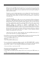
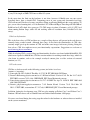
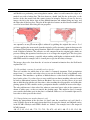
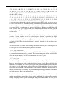
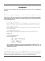
2.3.3 removing triangulation from v6.contourf and contour functions
Another issue with these plots was that the original data had too low of resolution for the plots
CDS user manual
page 6
and Matlab was performing some triangulation routine, where it would connect the edges of a
masked area with a broken line. The data, however, should look like the pcolor plot; so the
borders of the data would look like squares instead of triangles. Below you can see the two
images: the left as the before shot of using Matlab functions and without fixing any bugs, and
the other after all the bug fixes. The plot on the right also features an added border around it and
as well as better labels after fixing the text properties.
The squareness of the plot on the right is achieved by gridding the original data on to a 2n+1
grid after applying the ocean mask, from the original n grid by inserting a point in-between each
re-computed data point using interp2 function, which also results in smoother contour lines as a
result of higher resolution. The statistics are still computed from the original grids which are
preserved during this operation, but what you see is no longer the original grid. This does place
a lot of strain in the memory, especially when working with higher resolution models like the
n90 GFDL model for example, but it's a small price to pay for the clarity of images.
The images above also show how the v6 version of contourf.m function fixes the NaN mask
explained in 2.3.1.
2.3.4 Logarithmic contours for variables such as 'precip'
There are variables for which data at low values is extremely important. Total precipitation
ranges from 0 – n mm/day and values close to zero can be looked at using a logarithmic scale
for contours. This introduces a problem, as Matlab chooses a color from an available colormap
based on the values. So, values closer to zero would have an almost matching color and would
be hard to differentiate between. Professor Kushner's idea was to plot the powers of two and
then re-label the plot with the real data values. After tweaking the text properties and adding this
plotting option to CDS variables such as precipitation became available in better color ranges.
The only problem now is that values 0 to whatever your most lowest value in the contours are
shown as white space, as they are outside the plotting range. This might be fixed, if enough
users consider that white space in the plots is redundant. However, it is reasonable right now to
leave this as white space for the release.
2.3.5 Interpolations onto another dataset's grid
During the interpolation of the first data set (data1) onto the second data set's grid (data2) a
series of NaNs appear in the newly-interpolated data, because the latitude and longitude arrays
in the NCAR's reanalysis and GFDL's model are “shifted”. For example, here is the output of
NCAR's latitude:
-90, -87.5, -85, -82.5, -80, -77.5, -75, -72.5, -70, -67.5, -65, -62.5, -60, -57.5, -55, -52.5, -50,
CDS user manual
page 7
-47.5, -45, -42.5, -40, -37.5, -35, -32.5, -30, -27.5, -25, -22.5, -20, -17.5, -15, -12.5, -10, -7.5, -5,
-2.5, 0, 2.5, 5, 7.5, 10, 12.5, 15, 17.5, 20, 22.5, 25, 27.5, 30, 32.5, 35, 37.5, 40, 42.5, 45, 47.5,
50, 52.5, 55, 57.5, 60, 62.5, 65, 67.5, 70, 72.5, 75, 77.5, 80, 82.5, 85, 87.5, 90 ;
and this is GFDL's latitude:
-89, -87, -85, -83, -81, -79, -77, -75, -73, -71, -69, -67, -65, -63, -61, -59, -57, -55, -53, -51, -49,
-47, -45, -43, -41, -39, -37, -35, -33, -31, -29, -27, -25, -23, -21, -19, -17, -15, -13, -11, -9, -7, -5,
-3, -1, 1, 3, 5, 7, 9, 11, 13, 15, 17, 19, 21, 23, 25, 27, 29, 31, 33, 35, 37, 39, 41, 43, 45, 47, 49,
51, 53, 55, 57, 59, 61, 63, 65, 67, 69, 71, 73, 75, 77, 79, 81, 83, 85, 87, 89.
As you can see, not only are the values in Reanalysis go over GFDL's grid, but also the rest of
the values do not match. So, when interpolating using Matlab's griddata function, after meshing
the linear to 2D arrays with meshgrid, the values that fall outside the latitude/longitude range
get assigned NaNs. A workaround was proposed by Professor Kushner to pad the data with
itself. Basically, data1 gets wrapped around itself in longitude and latitude directions, and the
arrays also get wrapped around and increased in size before the interpolations step to fill in the
missing values.
This currently lacks full functionality. First of all, while this technique works in the latitude
direction, it is not clear how to do this in the longitude direction to get rid of the NaNs.
Secondly, if the grids change to something else, then the code might be rendered obsolete. For
now, this does not pose a huge threat to CDS for the first release as the statistics functions filter
out bands of NaNs. The statistics should not be affected, although this has not been tested
formally yet.
This whole section only matters when working with data on different grids. Comparing data on
the same grids was tested formally and no problems were found.
2.3.6 M_Map modifications
After fixing the issues described in sections 2.3.1-2.3.2 Max decided to modify M_Map's
m_contourf function into my_v6_m_contourf. This function incorporates all the fixes described
above but only for M_Map. This was tested informally on a series of plots.
2.3.7 'pcolor' plots
During the development of CDS there was a time when the 4 types of plots described above
were also available in pcolor, before the issues with the rest of the plots were resolved.
However, those plots never made it to the final release because, firstly, they would add to the
confusion, as already there are a lot of types of plots being generated by other plotting software,
and secondly, the size of the squares generated by pcolor would confuse the user, as they do not
represent the true resolution of the data, because of the colormap limitations. Basically when we
limit the colors used by the colormap, the pcolor function performs approximations to make the
plot look smoother, which is not in our interests.
The files from the development are in 'not_included_in_release' folder, and Max is currently
working on publishing some of these files as utilities on Matlab File Exchange. For example,
multiple colopmaps can be applied to one figure using video output, which was also part of
CDS user manual
page 8
CDS's functionality for pcolor that also didn't make it to the final release.
2.3.8 netCDF and mexCDF interface
It was decided to include mexCDF and netCDF as part of Matlab. This, however, is not so
simple.
While
the
netCDF
folder
can
be
acquired
from
http://woodshole.er.usgs.gov/staffpages/cdenham/public_html/MexCDF/nc4ml5.html and then
simply included into Matlab path, like M_Map during CDS execution, mexCDF has to be
compiled for the platform that you are running CDS on. After extensive testing, Max decided to
compile a Linux mexCDF binary and a Mac OS mexCDF binary and include them as part of
CDS. Since Matlab knows which OS it's running on, it can then determine which binary to use.
This was not tested formally, due to a lack of knowledge about the Matlab kernel. However,
pre-compiled binaries with netCDF 3.5.1 libraries worked so far on all tested platforms, so there
is no reason to believe why they should not work on any other Linux or Macintosh machine.
Other pre-compiled binaries on netCDF 3.5.0 libraries are available from the site mentioned
above, in case your version of CDS starts complaining that it can't open a certain netCDF file.
The binaries are located in CDS/dependencies/mexcdf. Simply replace the binaries that come
with CDS with your binaries if you need to.
2.3.9 Other modifications
During the development, 'usercolormap' function was borrowed from the Matlab File Exchange
and other functions that control the ticks of the labels and some averages and masks were
borrowed from Professor Paul Kushner. 'usercolormap' uses a custom gamma that generates a
red to blue colormap with a dirty-light-gray color at the transition, thus reserving pure white
color for NaNs only.
There were a lot of other worked-around issues during the development of CDS, but the author decided
not to include them into this manual due to their insignificance.
2.4 How to add your variables to CDS
As mentioned in the introduction, CDS reads the files under plots/vars folder. Each folder has the same
name as the file inside it, which describes the variable and the plotting function being performed. The
user is encouraged to look at create_vars.csh script for guidance on how each file is created or to at
least run the script a couple of times to generate their own variable templates (see 1.3.2). Basically,
each file presets certain data, which is then handed over to CDS for plots and analysis. Each file returns
the data being plotted, a contour array from each plot, the type of plot as a string, a boolean for
logarithmic scale, figure name, and x-y range. Variables such as logscale, xlim and ylim are being used
differently by handle_vars.m script, depending on the plot type being generated.
'logscale' variable toggles the logarithmic scale on the pressure axis for longitude-pressure/latitudepressure plots and it also toggles the logarithmic color scale for longitude-latitude plots, but it does
nothing for M_Map polar plots for now. Xlim and ylim variables establish plotting regions for all plots,
but differently. Ylim controls the number of latitude degrees away from the poles for M_Map plots, the
CDS user manual
page 9
averaging region for longitude-pressure plots and runs -90:90, while xlim does nothing for these plots.
For longitude-latitude plots, xlim and ylim work together to establish the plotting region, and are in the
range 0 xlim 360 and -90 ylim 90. For latitude-pressure plots both variables do nothing thus
far.
Each variable setting file also protects the variable by looking for it first in the list of variables supplied
by each netCDF file. If the variable is not found in this list, then CDS simply omits the variable-setting
file, prints a message to the screen and continues running.
The user is free to add any other operations on the extracted data in the if/end statement that checks for
existence of a variable. The user can also add their own function for extracting the data from the
netCDF file and averaging it. The extraction files thus far are: ssnm.m, ssnm_at_level.m,
ssm_zm_xlongitude_ypressure.m and ssm_zm_xlatitude_ypressure.m. You can refer to the
documentation of these files to find out what they do and which other files they call.
2.5 Testing CDS functions
While most of the functions were tested visually by playing around with different plots, the
interpolation and statistics functions could not be tested this way. So, in the testing directory one can
find 'interpolations.m' and 'statistics.m' files that test those functions at the Matlab command prompt.
The issues with different grids with the interpolations are well-aware of (see 2.3.5). The statistics
functions also have a flaw if a variance of a variable is a perfect zero, in which case division by zero
occurs twice in the correlation, which results in a NaN. However, the probability of getting a prefect
zero variance is negligible.
CDS was also tested by comparing CDS-generated images to images generated with GrADS and Ferret
software.
CDS user manual
page 10
CDS in more detail
This section deals with hardware and software functionality of CDS, as well as any mathematical
operations.
3.1 Statistics
CDS is able to compute three different types of statistics, for the different plot types. Each of these has
a hardcoded threshold of 0.5 for NaN tolerance, which means that a vector with more then half of it's
values as NaNs is not processed. NaN values are also not being processed. Functions in CDS/utilities
folder starting with “stats”in the filename are responsible for this. Please refer to the comments in these
files for computational details.
3.1.1 Longitude and Latitude plots
Here the weighting is done only by the cos of latitude, because closer to the poles the latitude
bands cover less surface area than at the equator. M_Map and coastal plots use these statistics.
3.1.2 Latitude and Pressure plots
Here the weighting is done by cos of latitude and change (delta) in pressure and this is used by
pressure vs latitude plots.
3.1.3 Longitude and Pressure plots
Here the weighting is done only by change (delta) in pressure and is used by pressure vs
longitude plots.
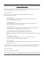
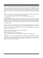
3.1.4 The computational formulas
The main formulas use are:
,
where A is the Nlev x Nlat matrix, p is the pressure vector and Phi is the latitude vector. In the
case of longitude, the second formula becomes the mean between two data points and the
longitude vector is not used.
3.2 Hardware Support: OpenGL
Although usually related to working with dynamic 2D and 3D graphics, such as for example video
games, Direct Rendering is an important part of CDS. This section has only been tested for Linux
platforms, because firstly Macintosh computers have 100% hardware support from the kernel and thus
usually have this working and secondly there was no clear way of testing this for Mac OS.
CDS user manual
page 11
If you are using a Linux system and would like to know if your video card is working properly, then
you can execute “glxinfo | grep -i direct”. If the line says something like 'direct rendering: Yes', then
you are fine. What this means is that your kernel and your X session can use the hardware acceleration
provided by the video card. So, when Matlab needs to generate a CDS image, instead of emulating a
video card, it can use the video card on your computer, thus reducing CPU load and reducing running
time.
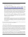
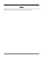
There are commonly 2 types of hardware accelerations: 2D and 3D. So, for example, if I want to rotate
a point (1, -1) in 2D to (1, 1), then I would multiply the rotation matrix
with Theta
by (1, -1). This can be done by your video card,
and this is actually the primary function of AGP (Accelerated Graphics Port) in your computer's
motherboard for 2D and 3D data points. Matlab can switch to your video card while rendering images
using OpenGL hardware API. Usually, if you have Direct Rendering, Matlab should have no problem
using any of the OpenGL extensions that you have to render the images. CDS sets the Matlab renderer
to OpenGL by default.
One way to test this is to run 'glxgears' in Linux and see how much strain you have on the CPU and
how much FPS you are getting . If glxgears reports no problems then Matlab should be able to use your
hardware video acceleration. As a benchmark test, you can run 'bench' in Matlab to see how your
system compares to other systems.
Sometimes you might get the following message during Matlab start:
Warning: Could not query OpenGL.
Warning: OpenGL appears to be installed incorrectly.
In this case, CDS might still run, but the author takes no responsibility in case CDS crashes.
WARNING: if you do not have OpenGL hardware acceleration, then CDS might crash with a
segmentation fault. If you have a powerful system then this might not happen, but for a system with
slower CPU and smaller RAM the probability of obtaining a segmentation fault is high. Usually this
happens during the image rendering process.
CDS user manual
page 12
Afterword
Thank you for using the first release of CDS. If you have any questions, concerns or suggestions
regarding this package, please feel free to e-mail max@atmosp.physics.utoronto.ca