1
xprafts
URBAN & RURAL RUNOFF
ROUTING SOFTWARE
xpsoftware
Head Office
8-10 Purdue Street
Belconnen ACT 2617
Postal Address:
PO Box 3064
Belconnen ACT 2616
Reference Manual
Phone : (02) 6253 1844
Fax (02) 6253 1847
Table of Contents
xprafts................................................................................................................................................................................ 1
1 - An Overview ................................................................................................................................................................. 3
AN XP OVERVIEW
3
THE MODEL STRUCTURE 3
PHILOSOPHY
3
STRATEGY
4
Graphical User Interface
4
The Graphical User Interface ...................................................................................................................................... 4
The Window................................................................................................................................................................ 4
The Menus ................................................................................................................................................................. 5
The Pointing Device.................................................................................................................................................... 6
Icons........................................................................................................................................................................... 6
2 - Building the Network................................................................................................................................................... 10
BUILDING THE NETWORK 10
GRAPHICAL ELEMENTS
10
CREATING A NETWORK 10
NAMING AN ELEMENT
11
CREATING A BACKGROUND
12
SELECTING AN OBJECT 12
MOVING OBJECTS
13
RECONNECTING OBJECTS
DELETING OBJECTS
13
13
THE COORDINATE SYSTEM
13
TRAVERSING THE NETWORK
13
PANNING AROUND THE NETWORK 13
RE-SCALING THE NETWORK WINDOW
13
The Scale Menu Command 14
The Scaling Tools
14
Window Scaling 14
Fit Window
14
RE-SIZING THE BACKGROUND
14
RE-SIZING NETWORK OBJECTS
15
Background Images
17
Importing Background Pictures ................................................................................................................................. 17
File Type................................................................................................................................................................... 18
Destination Rectangle............................................................................................................................................... 18
Edit Background ....................................................................................................................................................... 18
Hints on Background Picture Creation ...................................................................................................................... 19
Input File................................................................................................................................................................... 20
HPGL File Format..................................................................................................................................................... 20
XP Metafile ............................................................................................................................................................... 21
i
Table of Contents
XP Metafile Output File ............................................................................................................................................. 21
3 - Database Concepts .................................................................................................................................................... 22
DATABASE CONCEPTS
22
Database Concepts
22
THE DIALOG BOX ................................................................................................................................................... 22
THE PERMANENT DATABASE ............................................................................................................................... 22
THE WORKING DATABASE .................................................................................................................................... 22
DATABASE INTEGRITY........................................................................................................................................... 23
4 - The Copy Paste Buffer ............................................................................................................................................... 26
USING THE COPY BUFFER
26
Using the Copy Paste Buffer
26
COPY DATA FROM A SINGLE OBJECT ................................................................................................................. 26
COPY A SINGLE ITEM............................................................................................................................................. 26
Copy a Dialog List (DLIST) Item................................................................................................................................ 27
COPYING GLOBAL DATA........................................................................................................................................ 27
5 - Customizing xprafts .................................................................................................................................................... 31
CUSTOMIZING xprafts
The .ini File
31
31
XP-RAFTS.INI FILE.................................................................................................................................................. 31
OPT_DB_KEY .......................................................................................................................................................... 32
OPT_RAF_NODE_ADV_BTN................................................................................................................................... 32
OPT_RAF_SIMPLE_OSD_ADV_BTN ...................................................................................................................... 32
OPT_DB_MEM......................................................................................................................................................... 33
OPT_REDRAW ........................................................................................................................................................ 33
OPT_IDX_ACCESS.................................................................................................................................................. 33
OPT_DIRTYOBJ....................................................................................................................................................... 33
IO_BUF_SIZE........................................................................................................................................................... 34
OPT_PART_REC ..................................................................................................................................................... 34
MAX_NODES ........................................................................................................................................................... 34
MAX_TEXTS ............................................................................................................................................................ 34
MAX_PICTS ............................................................................................................................................................. 34
MAX_LINKS ............................................................................................................................................................. 35
MAX_DBCARDS ...................................................................................................................................................... 35
DATE_FORMAT....................................................................................................................................................... 35
CACHE_SIZE ........................................................................................................................................................... 35
APP_FLAGS............................................................................................................................................................. 35
PROJECTS .............................................................................................................................................................. 36
EDITOR.................................................................................................................................................................... 36
TEMPDIR ................................................................................................................................................................. 36
ENGINE.................................................................................................................................................................... 36
DIRECTORY ............................................................................................................................................................ 36
File Extenstions 37
FILE EXTENSIONS .................................................................................................................................................. 37
ii
Table of Contents
6 - Toolstrip Icons ............................................................................................................................................................ 38
THE TOOLSTRIP ICONS
POINTER
38
Moving Objects
38
Reconnecting Links
38
38
NODE 39
LINK
39
Polylink39
SCALING TOOLS
39
7 - Menus ........................................................................................................................................................................ 42
THE MENU BAR 42
All Nodes
42
All Links
42
Settings
43
Export To DXF
43
Calibrate Model 43
Encrypt for Viewer
Review Results
43
Spatial Report
44
Location
45
Text Size
46
Creation
46
43
Redraw46
Save Report
46
Load Report
46
Data Variables (Link)
46
Delete 47
Insert/Append
47
Format 48
Text Formatting 48
Text Attributes
49
Frame Display (Links)
49
Frame 50
Colour....................................................................................................................................................................... 50
Line Type.................................................................................................................................................................. 50
Width - ...................................................................................................................................................................... 50
Automatic ................................................................................................................................................................. 50
Box Width ................................................................................................................................................................. 50
Hide.......................................................................................................................................................................... 50
Type - ....................................................................................................................................................................... 50
Box ........................................................................................................................................................................... 50
Opaque..................................................................................................................................................................... 50
Bracket ..................................................................................................................................................................... 50
iii
Table of Contents
Attachment Line 50
Data Variables (Node)
51
Delete 51
Insert/Append
51
Format 52
Text Formatting 52
Text Attributes
53
Frame Display (Nodes)
53
Format 53
Attachment Line 54
Display Report
Hide
54
55
Show 55
Object Filter
55
Object Selection 55
Encode55
Restore
Load
55
Save
55
55
Cancel 55
Preferences
55
Hide Arrows .............................................................................................................................................................. 55
Fill Nodes ................................................................................................................................................................. 55
Hide Link Labels ....................................................................................................................................................... 56
Legend 56
Arrange Items
56
Window Legend 56
Network Legend 56
Variable
57
Visual Entity
57
Node Colour
58
Suggest - .................................................................................................................................................................. 58
Node Size
58
By Equation
59
By Linear Relationship
Size
60
60
Suggest
61
Graph 61
Node Label Size 61
By Equation
61
By Linear Relationship
Size
63
Suggest
iv
63
62
Table of Contents
Graph 63
Link Colour
63
Suggest - .................................................................................................................................................................. 64
Graph 64
Link Width
64
By Equation
64
By Linear Relationship
Size
65
66
Suggest
66
Graph 66
Link Label Size
66
By Equation
67
By Linear Relationship
Size
68
68
Suggest
68
Graph 68
THE WINDOWS MENU
68
THE HELP MENU
68
File
71
THE FILE MENU ...................................................................................................................................................... 71
New .......................................................................................................................................................................... 72
Open ........................................................................................................................................................................ 73
Close ........................................................................................................................................................................ 74
Save ......................................................................................................................................................................... 74
Save As Template .................................................................................................................................................... 74
Save As .................................................................................................................................................................... 75
Revert....................................................................................................................................................................... 75
Import Data............................................................................................................................................................... 75
Spreadsheet Import .................................................................................................................................................. 75
Import External Databases........................................................................................................................................ 76
Export Data............................................................................................................................................................... 81
Object Selection 82
Variable Selection..................................................................................................................................................... 82
Print.......................................................................................................................................................................... 83
Print Preview ............................................................................................................................................................ 83
Print Setup................................................................................................................................................................ 83
Exit ........................................................................................................................................................................... 83
Import ....................................................................................................................................................................... 83
Recent Files.............................................................................................................................................................. 83
XPX .......................................................................................................................................................................... 84
Edit
87
THE EDIT MENU...................................................................................................................................................... 87
Cut Data ................................................................................................................................................................... 88
v
Table of Contents
Copy Data ................................................................................................................................................................ 88
Paste Data................................................................................................................................................................ 88
Clear Data ................................................................................................................................................................ 88
Delete Objects .......................................................................................................................................................... 89
Edit Data................................................................................................................................................................... 89
Attributes .................................................................................................................................................................. 89
Font .......................................................................................................................................................................... 91
Node Name .............................................................................................................................................................. 91
Notes........................................................................................................................................................................ 91
Edit Vertices ............................................................................................................................................................. 92
Project 92
THE PROJECT MENU ............................................................................................................................................. 92
New .......................................................................................................................................................................... 93
Edit ........................................................................................................................................................................... 94
Close ........................................................................................................................................................................ 94
Save ......................................................................................................................................................................... 94
Save As .................................................................................................................................................................... 94
Multi-Run .................................................................................................................................................................. 95
Multi-Run .................................................................................................................................................................. 96
Details ...................................................................................................................................................................... 96
View
97
THE VIEW MENU..................................................................................................................................................... 97
Previous ................................................................................................................................................................... 98
Fit Window................................................................................................................................................................ 98
Redraw98
Set Scale .................................................................................................................................................................. 98
Grid .......................................................................................................................................................................... 98
Lock Nodes............................................................................................................................................................... 98
Find Objects ............................................................................................................................................................. 99
Select Objects .......................................................................................................................................................... 99
Toolbar ..................................................................................................................................................................... 99
Status Bar................................................................................................................................................................. 99
Network Overview..................................................................................................................................................... 99
Background Image.................................................................................................................................................... 99
Results 103
THE RESULTS MENU............................................................................................................................................ 103
Browse File............................................................................................................................................................. 103
XP Tables............................................................................................................................................................... 104
Graphical Encoding ................................................................................................................................................ 104
Configuration
105
THE CONFIGURATION MENU .............................................................................................................................. 105
Job Control ............................................................................................................................................................. 106
Global Data............................................................................................................................................................. 106
vi
Table of Contents
Units ....................................................................................................................................................................... 107
Tools
108
THE TOOLS MENU................................................................................................................................................ 108
Analyze
108
THE ANALYZE MENU............................................................................................................................................ 108
Solve ...................................................................................................................................................................... 109
Show Errors............................................................................................................................................................ 110
Pop-Ups
110
THE POP-UP MENUS ............................................................................................................................................ 110
8 - Node Data ................................................................................................................................................................ 111
NODE DATA
111
Direct Input
113
File Input
114
Output Control
114
Hydrograph Export
Use Baseflow
115
116
Tailwater Initial Rating
117
Rafts Storm Name
118
Hydsys Prophet Storm Name
Basin General Data
118
Gauged Hydrograph
120
118
Gauged Hydrograph ............................................................................................................................................... 120
Gauged Rafts Hydro ............................................................................................................................................... 121
Gauged Hyd Prophet Hydro.................................................................................................................................... 122
Gauged Stage Discharge........................................................................................................................................ 122
Retarding Basin 123
Retarding Basin ...................................................................................................................................................... 123
Basin General Data
124
Basin Storage ......................................................................................................................................................... 125
Upper Outlet ........................................................................................................................................................... 126
Floor Infiltration....................................................................................................................................................... 127
Outlet Optimization ................................................................................................................................................. 128
Normal Spillway...................................................................................................................................................... 129
Fuseplug Spillway................................................................................................................................................... 130
Basin Tailwater ....................................................................................................................................................... 130
Spillway Rating Curve............................................................................................................................................. 132
Conduit Discharge .................................................................................................................................................. 132
Basin Stage discharge............................................................................................................................................ 134
Sub-Catchment Data
134
SUB-CATCHMENT DATA ...................................................................................................................................... 134
Rainfall Losses ....................................................................................................................................................... 137
Ten unequal sub areas ........................................................................................................................................... 138
Direct Storage Coefficient ....................................................................................................................................... 139
vii
Table of Contents
Catchment Properties ............................................................................................................................................. 139
First sub-catchment ................................................................................................................................................ 140
Non std storage exponent ....................................................................................................................................... 141
Rainfall Loss Method .............................................................................................................................................. 141
Second sub-catchment ........................................................................................................................................... 142
Local Storm Name .................................................................................................................................................. 143
Use Baseflow
143
Simple On-site Detention/Retention ........................................................................................................................ 144
WSUD Onsite Detention/Retention ......................................................................................................................... 151
9 - Link Data .................................................................................................................................................................. 160
LINK DATA
160
LAGGING LINK DATA
160
ROUTING LINK DATA
160
Rafts Cross Section
162
Hec2 Cross Section
162
DIVERSION LINK DATA
163
Low Flow Pipe
165
DIVERSION LINK DATA
166
10 - Job Control ............................................................................................................................................................. 169
JOB CONTROL INSTRUCTIONS
Job Definition
169
171
Global Storm........................................................................................................................................................... 171
Catchment Dependent Storm.................................................................................................................................. 172
Automatic Storm Generator .................................................................................................................................... 173
Evaporation ............................................................................................................................................................ 174
Interconnected Basins ............................................................................................................................................ 175
Storm Type............................................................................................................................................................. 175
Global Hydsys Filename ......................................................................................................................................... 175
Results ................................................................................................................................................................... 175
Generate Data Echo ............................................................................................................................................... 175
Storage Coefficient Multiplication Factor ................................................................................................................. 175
Hydrograph Export
176
Local Hydrograph Export File.................................................................................................................................. 176
Total Hydrograph Export File .................................................................................................................................. 176
xpswmm/xpstorm Format Hydrograph Export File................................................................................................... 176
Summary Export File .............................................................................................................................................. 177
Simulation Details
177
Start Date ............................................................................................................................................................... 177
Start Time............................................................................................................................................................... 177
Use Hotstart File..................................................................................................................................................... 177
Create Hotstart File................................................................................................................................................. 178
11 - Global Data............................................................................................................................................................. 179
GLOBAL DATA
viii
179
Table of Contents
Global Database Records
181
RAFTS Storms ....................................................................................................................................................... 181
Hydsys/Prophet Storms .......................................................................................................................................... 182
Temporal Patterns .................................................................................................................................................. 183
Hydsys Hydrographs .............................................................................................................................................. 183
ARBM Losses......................................................................................................................................................... 184
Initial/Continuing Losses ......................................................................................................................................... 187
IFD Coefficients ...................................................................................................................................................... 188
Prophet Stage Data ................................................................................................................................................ 192
Stage/Discharge Data............................................................................................................................................. 193
XP Tables............................................................................................................................................................... 193
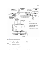
12 - PMP ....................................................................................................................................................................... 201
PMP
201
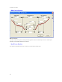
PMP Method Diagram
201
PMP Method Table
202
PMP Method Zones
203
GSDM 203
GSAM 203
GTSMR
204
13 - XP System.............................................................................................................................................................. 205
XP SYSTEM CAPABILITIES
205
NETWORK MANIPULATION
205
DATA TYPE
205
DATA RANGE CHECKING 205
RELATIONAL CONSISTENCY CHECKING
206
14 - RAFTS Theory........................................................................................................................................................ 209
Overview
209
Hydrology
209
Hydrograph Generation .......................................................................................................................................... 209
Rainfall ................................................................................................................................................................... 210
Loss Models ........................................................................................................................................................... 211
Storms .................................................................................................................................................................... 212
Gauged data........................................................................................................................................................... 213
Hydraulics
213
Transporting Hydrographs ...................................................................................................................................... 213
Hydrodynamic Modelling......................................................................................................................................... 214
Storage Basins ....................................................................................................................................................... 214
Importing Data
216
Importing Data ........................................................................................................................................................ 216
Output 216
Output..................................................................................................................................................................... 216
Graphical Output..................................................................................................................................................... 216
Tabular Reports...................................................................................................................................................... 216
ix
Table of Contents
Detailed Description of xprafts
217
General Model Structure......................................................................................................................................... 217
Program Organisation............................................................................................................................................. 217
General Data Requirements ................................................................................................................................... 219
Library Module (LIBM) ............................................................................................................................................ 219
Time Step Computations ........................................................................................................................................ 219
Definition of Link ..................................................................................................................................................... 219
Convergent and Divergent Links............................................................................................................................. 220
Development of Catchment, Channel & Network Data ............................................................................................ 220
Catchment Area Representation............................................................................................................................. 221
Treatment of Subareas ........................................................................................................................................... 221
Graphical & Tabular Output .................................................................................................................................... 222
Hydrograph Generation Module .............................................................................................................................. 222
Catchment Rainfall ................................................................................................................................................. 223
Design Rainfall Bursts............................................................................................................................................. 223
Historical Events ..................................................................................................................................................... 223
Continuous Rainfall Data ........................................................................................................................................ 223
Sub-catchment Rainfall Routing Processes ............................................................................................................ 223
Routing Method ...................................................................................................................................................... 225
Storage-Discharge Relationship.............................................................................................................................. 225
Coefficients B and n................................................................................................................................................ 226
B Modification Factors ............................................................................................................................................ 226
Rainfall Loss Module .............................................................................................................................................. 227
Initial and Continuing Loss Model ........................................................................................................................... 227
Retarding Basin Module.......................................................................................................................................... 228
Routing Details ....................................................................................................................................................... 229
Basin Stage/Storage Relationships......................................................................................................................... 230
Basin Stage/Discharge Relationships ..................................................................................................................... 230
Basin Outlets .......................................................................................................................................................... 231
Link/Conduit Module ............................................................................................................................................... 231
Phillip's Infiltration Module....................................................................................................................................... 232
Impervious and Pervious Areas Loss Parameters................................................................................................... 238
15 - References ............................................................................................................................................................. 241
REFERENCES
241
Index ............................................................................................................................................................................. 245
x
xprafts
No Data
1
1 - An Overview
AN XP OVERVIEW
The practical implementation of any project involving storm and wastewater management is not a trivial task.
Depending on the degree of complexity it may require an expert hydrologist knowledgeable in modelling techniques,
and a hydraulic expert knowledgeable in the modelling of free surface and pressure flow networks. It may also require
the expertise of an environmental engineer to assess pollutant buildup, wash-off and diffusion and a computer
specialist to prepare the data files and coordinate the execution of various modules of the computer program.
It requires the coordinated efforts of all these "experts" to select the appropriate modelling options, to select
appropriate values for input parameters, and to evaluate and interpret model output and to diagnose possible
malfunctions of the drainage system and suggest remedies.
In actual projects, depending on the complexity of the problem, the calibration work can take several weeks or more.
The XP environment is designed to minimise (but not eliminate) the need for human "experts" and to guide the
Engineer or Scientist through the intricacies of a particular numerical model. Its aim is to improve productivity by
increasing the efficiency of data entry; eliminating data errors through expert checking and the using decision support
graphics and interpretation tools. The entire suite of tools creates a decision support system for the numerical model.
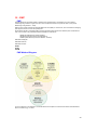
The main components of the XP model are THE GENERIC GRAPHICAL USER INTERFACE, THE MODEL
STRUCTURE, PHILOSOPHY, and the STRATEGY
THE MODEL STRUCTURE
The XP environment maintains a loose coupling to the analytical model and graphical and textual post-processors, via
text and binary data files. These data files are generated from the XP database when the "Solve" menu command is
issued and from the analytical engine when the network is analysed.
When the "Solve" command is given, XP first performs the high-level database integrity checks as described in the
documentation. If these checks are passed successfully and the model data files are generated, XP then performs the
task of running the analytical engine to process the data files and generate output for the graphical post-processors to
use.
When the analytical engine has completed its run any errors or warnings encountered in running the model are
reported and the user is placed back in the editing environment. The model results for a selection of objects can then
be viewed by using several graphical tools and reviewing text output files. Several utilities also exist for the export of
model results and data to GIS, spreadsheets or other databases.
PHILOSOPHY
An expert system is "a knowledge-based reasoning system that captures and replicates the problem-solving ability of
human experts" (Boose 1986) and typically has three basic components:
a knowledge base,
an inference engine, and
a working memory.
The knowledge base is "the repository for information that is static and domain-wide" (Baffaut et al 1987). The
knowledge base may contain not only static data that will not change from one problem to the next, but may also
contain empirical and theoretical rules, and provide advice on models that may be employed as part of the solution.
The inference engine is "the reasoning mechanism containing all the procedures for manipulating, searching, and
exercising the knowledge base" (Baffaut et al 1987).
The working memory is used to solve a specific problem using the expert system. It consists of the user interface to
the expert system and the storage of specific problem information. The working memory also serves as the
explanation device for the expert system indicating legal and illegal data and suggesting parameters.
A computer-based expert system has advantages over a human expert that include:
An expert may retire and knowledge is lost.
There may be better uses of an expert's time than answering user questions.
Expertise may be expensive to deliver.
An expert may not be available when needed.
An expert is not always consistent.
3
Printed Documentation
In any particular application these reasons or others may be important in deciding to use an expert system.
Expert systems development has created the need for a specialist called a knowledge engineer. Knowledge
engineering is "the extraction, articulation and computerisation of expert knowledge. Knowledge consists of
descriptions, relationships, and procedures in the domain of interest" (Boose 1986). The knowledge engineer provides
the interface between the human expert and the computer.
It is generally agreed that one of the largest, if not the largest, problem in expert systems development is knowledge
acquisition and knowledge engineering.
XP diverges from the traditional expert system by allowing the continuous accumulation of localised expertise to be
used within its shell with little assistance necessary from the software developer. The coupling of the Storm Water
Management Model to the XP interface with all of its graphical tolls has created a Decision Support System (DSS) for
storm and wastewater management.
STRATEGY
The graphical XP environment is, in essence, a shell that acts as an interpreter between the user and a model. The
XP graphical interface provides the user with a very high-level interface to various numerical simulation programs
oriented towards solving problems that may be represented as some form of link-node structure.
The main theme of this interface is Decision Support Graphics. At the front end of the interface the process of creating
data for the model is made as visual as possible, with the aim of emulating real world problems as closely as possible.
For example, most dialogs contain graphics that visually link the data being entered to the physical system being
modelled.
The user is given continual guidance and assistance during data entry. For parameters that are difficult to estimate,
the user may be advised of literature to aid in selecting a value, or an explanation of a parameter and some proposed
values may be shown on the screen. If there are other ways to pick the value, typically, if the parameter is a function
of other variables, the equation is shown to the user.
The user interface is intelligent and offers expert system capabilities based on the knowledge of the software
developers and experienced users. For example, as various graphical elements are connected to form a network, XP
filters the user's actions so that a network that is beyond the scope of the model is not created. The general
philosophy is to trap any data problems at the highest possible level - at the point the users create the data.
At the back end of the user interface the results of model analysis and design are presented graphically to maximize
comprehension, assist in the interpretation of results and support decision-making.
Graphical User Interface
The Graphical User Interface
The generic graphical user interface utilizes the current Windows, Icons, Menus and Pointing device technology as the
state-of-the-art intuitive user environment.
The user interface can also be described as object-oriented. A user first selects an object or range of objects using
the pointing device, and then performs an operation on the selection by giving a menu command. For example, to
delete a group of objects they are first selected with the mouse and the "Delete Objects" command is selected from
the Edit Menu.
The XP interface may be used to create a new infrastructure network as well as to edit an existing one. The XP user
interface is object-oriented, which means the user selects the object, then selects the operation to perform on it.
The XP environment consists of:
A window with a series of menus along the top of the screen used for controlling operation of the program.
Several tool strips of icons for file operation, object creation/manipulation and short cuts to menu commands.
The elements of the interface and the method of manipulation of objects are described in the text below.
The Window
The Icons (The Toolbar)
The Menus
The Pointing Device
The Window
The Window provides the frame of reference for user interaction. The large display area provides a current view of the
created network of links and nodes. A Network Overview dialog provides a means of changing the position of the
4
1 - An Overview
current view of the network. The title of the current database (model) is displayed in the window title bar and status
messages describing current program activity such as a description of the function and mouse position are displayed
across the bottom of the window.
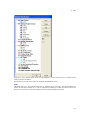
The Menus
The pull-down menu titles appear on a menu bar displayed underneath the window title. Each menu title represents a
group of related commands. If certain commands do not make sense in the current context of what the user is doing,
they are disabled and indicated by less prominent and shaded light gray.
The most frequently used commands also have keyboard equivalents, indicated by a keyboard combination such as
Ctrl+N (New) listed in the menu. Commands that require more information, typically entered via a Dialog Box, are
indicated with three trailing dots after the menu item name.
POP-UP MENUS
THE FILE MENU
THE EDIT MENU
THE PROJECT MENU
THE VIEW MENU
5
Printed Documentation
THE CONFIGURATION MENU
THE TOOLS MENU
THE ANALYZE MENU
THE RESULTS MENU
THE WINDOWS MENU
THE HELP MENU
The Pointing Device
The pointing device may be a digitizer, graphics tablet or a mouse. For the sake of consistency we use the term
mouse to indicate a generic-pointing device.
Throughout this manual various terms are used to describe functions performed using the mouse. Listed below is a
description of the basic mouse techniques used within this program.
Click
Position the pointer on something, and then briefly press and release the mouse
button.
Choose
Pick a command by positioning the pointer on the menu name, moving the
highlighted area down the menu to the command you want, and then clicking the
mouse button.
Drag
Position the pointer on or near something, press and hold down the mouse button as
you move the mouse to the desired position, and then release the button. You often
do this to move something to a new location or to select something.
Double click
Position the pointer on something, and then rapidly press and release the left mouse
button twice
Point
Position the left pointing arrow on or just next to something you want to choose.
Select
Move the cursor to an object, then click or drag across the object.
The mouse pointer changes shape to indicate the type of action that is taking place. The typical pointer icons are
described below:
Arrow Icon
You may select objects, move, re-connect or re-scale the network.
Node Icon
Nodes are being added to the network.
Link Icon
Links are being added to the network.
Diversion Icon
Overland flow diversion paths are being added to the network.
Text Icon
Nodes are being added to the network.
Polygon Icon
Lengths or areas are being measured from the network.
Window Icons
A background is being selected or the window is being panned or zoomed in or out.
Hourglass
Icon
XP is busy performing a task. The specific task is generally displayed in the status
messages area of the window.
Zoom-In Icon
You are currently zooming in to an area of the network.
Zoom-out Icon
You are currently zooming out on an area of the network.
The Mouse allows the user to select objects to operate on by pointing and clicking and similarly to initiate system
commands through Pull-down menus.
Icons
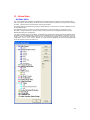
Icons
A palette of object symbols (Icons) is provided for the creation and manipulation of objects comprising the network.
These toolbars may be turned on and off by selecting Toolbar from the View Menu .
6
1 - An Overview
These tools compriseProject Icons
File and Print Icons
Tool Icons
Solve & Review Icons
Browse, and Help Icons
Background Picture Icons
Scaling Icons
Data Icons
Dialog Icons
Project Icons
This Toolbar is only enabled if Projects is enabled in the RAFTSXP.INI file.
New Project
This icon is used to create a new project database.
Open Project
This icon is used to open an existing project database.
See Also Project Menu .
File and Print Icons
This Icons in this Toolbar have slightly different functions depending on whether Projects is enabled in the
RAFTSXP.INI file.
New File
This icon is used to create a new database.
Open File
This icon is used to open an existing database.
Save File
This icon is used to save an existing database .
Print Network
Prints the current view of the network to the default Windows printer.
See Also File Menu .and Project Menu
Tool Icons
Pointer Tool
This tool is used to select objects, move objects, reconnect links, re-scale the window, change
object attributes and to enter data.
Text Tool
This tool is used to annotate the network by placing text objects on the network.
Node Tool
This tool is used to create nodes on the network. These may physically represent a manhole or
pit, an inlet for a catchment. The node shape changes to represent different physical
structures. Triangular nodes have storage properties in addition to the system defaults.
Basin Tool
This tool is used to create nodes on the network. These may physically represent a manhole or
pit, an inlet for a catchment plus a pond or retarding basin or a Best Management Practice
(BMP The node shape changes to represent different physical structures. Triangular nodes
have storage properties in addition to the system defaults.
Link tool
This tool is used to create a lagging link that joins two nodes in a network. This represents a
travel time down a reach but not the physical characteristics of the pipe or channel.
Channel tool
This tool is used to create a link that joins two nodes in a network. This link represents a
7
Printed Documentation
closed conduit such as a pipe or an open conduit such as a river or man-made channel.
Diversion tool
This tool is used to create a link that defines an overland flow path between two nodes in a
network.
Polygon tool
Used to measure the length of a polyline or the circumference and area of a polygon.
Select all
nodes
Selects all nodes in the model. Click on the white space to deselect.
Select all links
Selects all links in the model. Click on the white space to deselect.
See Also BUILDING THE NETWORK
Solve & Review Icons
These Icons provide shortcuts to the more commonly used menu commands.
Solve
Shortcut to the Solve command under the Tools Menu.
Review Results
Shortcut to the Review Results command under the Tools Menu.
Browse and Help Icons
Browse File
This icon provides a shortcut to the Browse File command under the Results Menu
Print Network
Prints the current view of the network to the default Windows printer.
Help
Load the xprafts.chm on-line help (this file!)
Background Picture Icons
The Icons in this Toolbar are used to manipulate any background pictures that may be present.
Get Picture
A shortcut to the Background Images command in the View Menu.
Picture
Properties
Edit the currently selected background picture.
Scaling Icons
The Icons in this Toolbar are used to change the scale or location of the current view of the network.
Redraw
Regenerates the network without changing the current location or scale.
Fit Window
Re-scales the network to fit the current window (Ft Window )
Pan
Move your view of the network by a user defined offset which is set by selecting this icon and
dragging the network from the old location to the new location.
Zoom In
Window
Magnify your view of the network by a user defined factor which is set by selecting this icon
and dragging a box around the area you wish to see.
Zoom Out
Window
Shrink your view of the network by a user defined factor which is set by selecting this icon and
dragging a box inside which the current view of the network will fit.
See Also Network Overview and Scaling Tools
Dialog Icons
These Icons are present on the right hand side of each dialog. They are used to get information on and to copy
individual fields including check boxes, radio buttons and editable text in a dialog.
8
1 - An Overview
Copy Data
Used to copy one field within a dialog so that it may be pasted into multiple nodes or links. See
also COPY A SINGLE ITEM. Select the item by dragging a box around a text item, radio button
or checkbox then select the Copy Icon
Help
Click this button to get help on the current dialog.
Field
Information
Used to get information on one field within a dialog so that it may be used in the creation of an
XPX file. Select the item by dragging a box around a text item, radio button or checkbox then
select the Field Information Icon
Data Icons
These icons provide shortcuts to the global and job control data and also to the data and results presentation options.
Global Data
Shortcut to the Global Data command under the Configuration menu
XP Tables
Shortcut to the XP Tables command under the Results menu
Graphical
Encoding
Shortcut to the Graphical Encoding command under the Results menu
Spatial Reports
Shortcut to the Spatial Reports command under the Results menu
Job Control
Shortcut to the Job Control command under the Configuration menu
9
2 - Building the Network
BUILDING THE NETWORK
This section of the manual describes the general philosophy behind the graphical XP environment and outlines the
basic design features of this package. It is a good starting point for any new users of any of the XP series of programs.
GRAPHICAL ELEMENTS
CREATING A NETWORK
NAMING AN ELEMENT
CREATING A BACKGROUND
SELECTING AN OBJECT
MOVING OBJECTS
RECONNECTING OBJECTS
DELETING OBJECTS
THE COORDINATE SYSTEM
TRAVERSING THE NETWORK
PANNING AROUND THE NETWORK
RE-SCALING THE NETWORK WINDOW
RE-SIZING THE BACKGROUND
RE-SIZING NETWORK OBJECTS
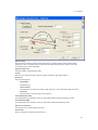
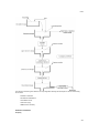
GRAPHICAL ELEMENTS
The major graphical objects consist of a series of links and nodes. The network of nodes is connected together by
links with some additional elements provided for annotation and background reference. The XP environment supports
the following types of objects.
Symbol
Name
Description
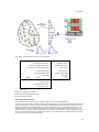
Node
Used to represent physical objects such as manholes, inlets, ponds, outfalls or junctions
of various links such as natural channels or closed conduits.
Link
Connections between nodes, they may be physical elements, or only indicative of a
connection eg. pipes, channels, overland flow paths, pumps, etc.
Text
Lines of text used for labelling purposes.
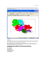
Picture
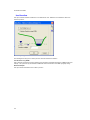
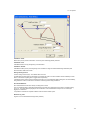
Bounded by a dashed rectangle a network backdrop is a pre-defined drawing, created
via a CAD package such as AutoCAD®, each background graphic is a single object.
Current background graphic types supported include HPGL, DXF and DWG
.
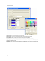
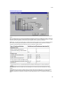
Each element of the network has certain editable spatial and display attributes and a unique name. Display attributes
include the colour and line thickness of the object. Five standard colours are supported; Black, Red, Green, Blue, and
Yellow. Three line thicknesses are provided: Thin, Medium and Thick. Spatial attributes include the position and
dimensions of the object. Digit images and text notes can also be attached to nodes through the attribute dialog.
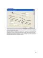
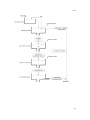
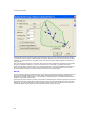
CREATING A NETWORK
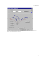
The network is created on the screen using the palette of tools (icons) contained in the tool strip in the window. To
create a network, select a node tool from the toolstrip by clicking it. The cursor shape now changes to a node object
symbol indicating a node is being created. Clicking in the window now defines the position of the node and creates it
and gives it a unique name. The display attributes of the new node (colour and thickness) are the same as those in the
toolstrip.
Next, create the links between nodes, selecting the link tool and then clicking on the nodes you wish to connect. The
cursor shape again changes to link object symbol indicating a link is being created. A link is directed from the first to
the second nodes clicked upon indicating the direction of flow from upstream to downstream. An arrow is placed on
10
2 - Building the Network
the downstream end of the link indicating the direction of positive flow. The position of the second end of the link (the
end towards which flows are directed) is indicated by a dotted outline which tracks the mouse movement. A default
unique name is automatically created for any object requiring a name.
You may create a polylink (bent link) by holding down the <Ctrl> key as you click with the mouse. This will create a
vertex at each point at which you click.
You may change an existing link to a polylink by holding the <Ctrl> key down and clicking at the locations where you
want a vertex.
You may remove a vertex by holding down the <Shift> and <Ctrl> keys and clicking on the vertex you wish to delete.
XP performs a series of validity checks to verify a legal network is being created and, if the connection satisfies all of
the rules, the link is created.
An additional feature of the link tool is the provision of a default end node. If the link tool is selected and you attempt to
create a link in free space, ie. you do not click on an existing node, a default node will be created. In this manner it is
not necessary to first create nodes and then join them with links, but rather perform both operations simultaneously.
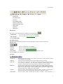
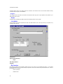
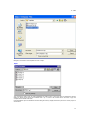
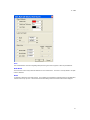
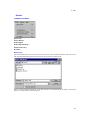
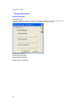
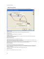
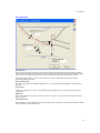
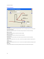
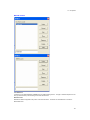
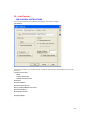
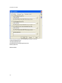
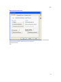
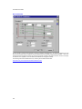
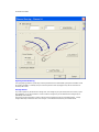
NAMING AN ELEMENT
Every object in the network must have a unique name. No node may have a name already used by another node or
link in the database. The names are limited to 10 characters. Three methods are available to name a network object,
the last two of which invoke the Attributes dialog box.
(i)
Highlight the node or link then click just below the name and modify the name directly on the screen. Follow the
editing with an enter keystroke to terminate editing.
(ii)
Highlight the node with the right mouse button and click. This will bring up a pop-up menu. Select Attributes to
enter the object name in the dialog.
(iii)
Highlight the node or link then select Attributes from the Edit menu.
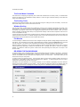
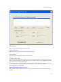
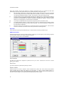
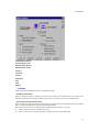
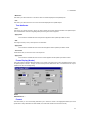
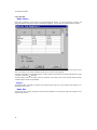
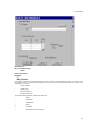
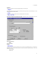
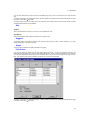
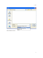
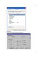
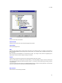
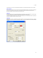
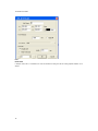
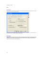
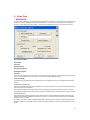
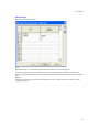
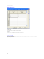
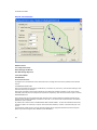
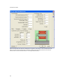
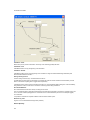
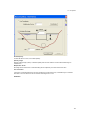
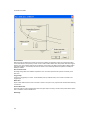
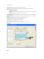
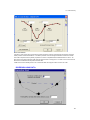
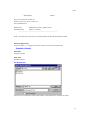
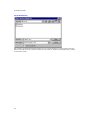
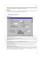
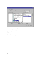
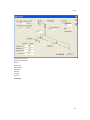
If method (ii) or (iii) above is chosen, a dialog box similar to that shown below is then displayed. If the object selected
is a link the coordinate boxes are not shown.
11
Printed Documentation
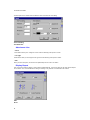
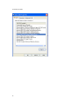
Picture File
A bitmap image can be attached to a node by entering the name of a graphics file in the Picture File field. The formats
currently supported are BMP, DXF, EPS, FAX, IMG, JPG, PCD, PCX, PNG, TGA, TIF, WMF, WPG, XBMP, XDCX,
XEPS, XJPG, XPCX and XTIF.
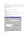
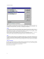
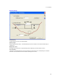
CREATING A BACKGROUND
Background pictures are special objects that can be created to act as passive backdrop on which the rest of the
network may be overlaid.
Pictures are stored in an internal graphics format, as files on disk. These “Picture” files must be present for the
background to be drawn. There is neither a limit to the number of background pictures that may be loaded into the
network nor to the size of an individual picture.
In general, these objects can be manipulated in the same way as any other network object, with the exception that the
<Ctrl> key must be used in conjunction with any other action. Thus, pictures can be selected, deleted, moved, hidden,
etc. A picture may be re-scaled isotropically by holding down the <Shift> and <Ctrl> keys.
Three background picture formats are supported: .DWG, .DXF and HPGL/1. DWG and DXF files are supported in
their native format. HPGL/1 files must be translated to a .PIC format using the supplied converter CVTHPGL.EXE.
See Also Importing Background Pictures
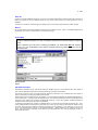
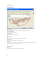
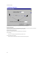
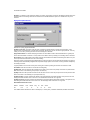
SELECTING AN OBJECT
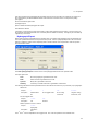
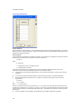
Many menu commands operate on the set of currently selected objects. An individual object is selected by choosing
the pointer tool from the tool strip, pointing at the object and clicking the mouse button. A selected object is indicated
by it being displayed with inverse highlighting.
Groups of objects can be selected by clicking in open space and with the mouse button held down dragging a dotted
rectangle around the group. If more than half the object is included in a rectangle the object is selected.
The selections can be extended to include or exclude objects by using the Shift key in conjunction with the mouse
button. It has the effect of toggling the state of the object between selected and unselected.
12
2 - Building the Network
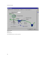
All the objects in the path between two end objects can be highlighted by clicking on the first node (or link), then, with
the Ctrl and Shift keys held down clicking on the second node (or link).
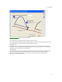
MOVING OBJECTS
A selected (highlighted) group of objects can be moved by dragging any object from the highlighted set - the rest will
follow. A dotted outline of all affected objects tracks the mouse movements until the button is released, indicating the
final position of the moved objects in real time.
RECONNECTING OBJECTS
A link can be reconnected to another node by first selecting it, then positioning the pointer near one end of the link and
dragging the end of the link to the new node. A dotted outline tracks the movement of the link in real time. Note: The
cursor retains the arrow shape.
Creation of the new link is subject to the same connectivity rules applied during network creation, ie. An illegal network
cannot be created through re-connection.
DELETING OBJECTS
A selected (highlighted) individual object or group of objects can be removed from the model by invoking the “Delete
Objects” menu command, from the Edit menu. Note: A link cannot exist without both end-nodes; thus when one endnode is removed, the link is also deleted. To delete a vertex from a polylink, hold down the <Shift> and <Ctrl> keys
and click on the vertex to be deleted.
A background picture is deleted by first selecting the file with the Select Background tool from the toolstrip. A selected
background is connoted with a hatched pattern. Invoking the delete background tool at this point will immediately
delete the background.
THE COORDINATE SYSTEM
The screen network is essentially open-ended and unbounded in any direction. The coordinate system has its origin
(0,0) at the lower left corner of the opening window and increases to the right and up. In the present implementation,
the coordinates are stored in double precision format with up to 20 significant figures to enable the retention of real
world coordinates. The coordinates are used in specifying the location of a node, text item, or the bounding rectangle
of a background picture.
TRAVERSING THE NETWORK
The network can be traversed by using the <Tab> key starting from any selected link or node. The <Shift-Tab> key or
key moves to the previous upstream object.
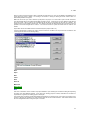
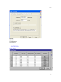
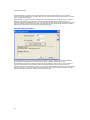
Alternatively the user may select “Go To ...” from the View Menu and enter the name of the required node or link. The
user may specify whether the search is for a node, link or text, or whether the object name is case sensitive or a partial
word search.
While employing the multi-selection option successive searches will add to the selection set.
When the user clicks Find the requested object name is searched for. If found it is highlighted and displayed in the
centre of the screen at the currently selected scale.
PANNING AROUND THE NETWORK
The user can pan by using the Pan tool from the toolstrip. First select the tool and positioning the mouse on a position
in the network to pan from. Then drag the mouse while holding down left mouse button to the new location for that
point. This moves the entire screen image the distance between the two points in the dragged direction.
While the user is performing this panning function a dotted "rubber" line is displayed showing the distance the image
will be moved and the direction.
RE-SCALING THE NETWORK WINDOW
When a network window is re-scaled the size of nodes and labels remains fixed, the nodes being symbols that
represent the centre of the object, or the junction of links. When the scale of a picture changes so that the text
becomes unreadable it is displayed as a black box showing the location of the text but not the actual characters. The
size of the viewed window can be changed in four ways:
The Scale Menu Command
The Scaling Tools
Window Scaling
Fit Window
13
Printed Documentation
The Scale Menu Command
The scale factor is a mapping or engineering form of scale with real-world units in metres (or feet). The default scale
at which the network of a new database is initially created is 1:1000. This type of absolute zooming is done about the
centre of the display window.
The Scaling Tools
Zooming can be performed relative to the current scale factor using the "scaling tools" from the toolstrip. The tools are
tied to fixed scaling of 2X for zoom in and 0.5X for zoom out.
Window Scaling
The size and location of a new window can be defined by zooming-in to a rectangle proportioned to the shape of the
display window. A rectangle similar to a selection rectangle is created by first selecting the Window Area In Tool from
the toolstrip and using the mouse button and dragging a rectangle around the area of interest. When the mouse
button is released, the window maps exactly to the proportioned rectangle. Both the size and position of the zoom box
can be manipulated in this way.
A zoom-out action may be performed in a similar manner by selecting the Window Area Out tool from the toolstrip and
following the above instructions. The dotted rectangle shown on the screen will indicate by how much the current full
window will be reduced and where the current window will be shown.
Fit Window
A “world rectangle” is defined as the minimum size rectangle enclosing all objects including background pictures and
text objects. The view window can be made to automatically fit the display by giving the Fit Window menu command
from the View Menu. This function is also embedded in the toolstrip by selecting the Fit to Window tool button.
When the window is zoomed in or out, the size of Nodes and Text may remain fixed relative to the screen or may be
scaled proportionally depending on whether the "Real-World size" or "Display size" option is chosen as the display
attribute. By default the nodes are symbols of fixed screen size representing the centre point of an object or the
junction of links.
RE-SIZING THE BACKGROUND
To select a picture, click on the Select Picture Tool from the toolstrip and click anywhere on the picture. The picture
will then be highlighted with a hatched pattern to indicate it has been selected. To move a picture first select it, then
continue to hold down the left mouse button and drag the picture to its new location. The location where you first
clicked is the “hot-spot” of the picture.
To resize a picture, first select the picture. With the mouse drag any of the picture “handles” located in the corner of
the picture or in the middle of each of the four rectangular line segments. A dotted rectangle tracks the mouse’s
movements and indicates the final size of the picture.
Alternatively the picture attributes, ie. its bounding rectangle, can be modified by highlighting the picture and then
selecting the Picture Properties from the toolstrip. This will cause the dialog box below to be displayed and new
coordinates may be entered. This dialog also contains a flag to show or alternatively hide the background drawing.
14
2 - Building the Network
Note that Backgrounds created from DXF or DWG files cannot be moved or re-sized.
RE-SIZING NETWORK OBJECTS
When a large network is displayed on the screen it can appear extremely cluttered. To allow the total network to be
viewed (and comprehended) the size of the text and objects may be tied to the scale of the displayed window.
When a group of objects is selected the following dialog boxes are displayed and the attributes such as colour, node
and text size etc., may be changed for the selected group of objects.
When OK is selected a dialog similar to the following is displayed (the dialog box shown is for a node selected above)
If Real World Size is selected, the text and object sizes are in real world units. When a scale too small to display is
selected the text will be drawn as a box and will only appear after zooming in. If display size is selected, text and
object sizes are set in decimal inches or millimetres independent of the scale selected.
The display font may be modified by selecting the corresponding font from a list. A preview of the font is displayed in
the Select Font dialog.
15
3 - Database Concepts
Background Images
Importing Background Pictures
Background pictures are special objects that can be created to act as passive backdrop on which the rest of the
network may be overlaid.
Pictures are stored as files on disk and only a reference to the file and the path is stored in the .XP file. These "Picture"
files must be present for the background to be drawn. There is neither a limit to the number of background pictures
that may be loaded into the network nor to the size of an individual picture. Pictures can be selected, deleted, moved,
hidden, etc
Five background picture types are supported: These include AutoCAD .DWG, and .DXF files, ESRI ArcView Shape
files, MapInfo MID/MIF files, digital photos such as .BMP, .JPG, .TIFF. and HPGL (HPGL/1) files which must be
translated to a .PIC (a native XP Software format) using the supplied converter CVTHPGL.EXE
To import a background select Background Image from the View Menu or click on the New Background Image tool.
DXF or DWG format:
To load a DWG or DXF file select XP Metafile as the file type and then hit the Select button for Input File. The
coordinates of the DWG/DXF file will be automatically used.
To create a picture file, a format conversion utility supplied with XP is invoked. This utility converts graphics from
HPGL into the internal format used by XP.
Note that Backgrounds created from DXF or DWG files cannot be moved or re-sized.
HPGL/1 format:
The background may also be imported from an HPGL/1 plot file that may be created via most CAD packages, or via
numerous design packages that provide output to Hewlett Packard plotters.
To create a background, an HPGL/1 plot file must be generated (from a CAD package, for example). This HPGL/1 file
is then converted to the picture format via the “CVTHPGL” utility supplied with XP. CVTHPGL is invoked from the Get
Background Menu.
The procedure involved in creating a picture from a CAD package is as follows (i)
Create the drawing in the CAD package;
(ii)
Ensure your CAD package is configured with a Hewlett Packard plotter for output. This must be in HPGL/1
format such as used for HP7580, HP7586, Draftsmaster etc. Newer Inkjet plotters like the HP650C, 700 series
17
Printed Documentation
etc can be configured to accept input in HPGL/2 format (the default) or HPGL/1 format. This converter cannot
use the HPGL/2 format.
(iii)
Plot the desired rectangle of interest, noting the co-ordinates of the boundaries. If you wish to retain the scale of
your drawing package then the XP destination coordinates must correspond to the top-left and bottom-right
corner (extreme points) of the drawing in your drawing package. It is also recommended to import your
background picture before creating a database.
(iv)
Select Get Background from the Special Menu and choose the HPGL format. When you select OK the
“CVTHPGL” program will convert the HPGL/1 file into the internal XP picture format (PIC).
File Type
HPGL
XP Metafile
Input File
Background
XP Metafile
Destination Rectangle
Notes:
(1)
An error log is created which lists any HPGL commands the program has been unable to translate.
(2)
The plotter defaults file "PL_DEF" defines the mapping of pen numbers to colours in a table at the
head of the file. The first line of the file contains the number of pens, the following lines contain the
mapping of pen number to colour name. Pen number zero, the null pen, must also be mapped to a
colour.
This pen colour transformation allows customization for particular CAD packages. See the default
file “PL_DEF” included with this program, for details.
(v)
Once the HPGL file has been converted to a picture file, it is incorporated into the network as an XP Metafile.
The user is prompted for the picture file name and destination bounding rectangle via the Get Background
dialog box.
By default, the bounding rectangle fills the display window at the currently selected scale. To maintain the original
proportion of the drawing, the user must recall the co-ordinates of the frame originally plotted and use these for the
destination-bounding rectangle.
File Type
The two file formats that can be imported are:
(a) XP Metafile - Internal XP picture file format. This is the file format used by XP to store its background pictures.
(b) HPGL - Hewlett-Packard File format. This file is usually created by configuring your CAD program (or other
drawing programs) to send the HPGL output to a file instead of the COM port.
The CVTHPGL utility will create a new XP Metafile. The filename of this new file will need to be specified.
Destination Rectangle
The outer corners (Top, Left, Bottom and Right) where the PICT file will be imported. If importing a HPGL format file
then the rectangle corresponds to the edges of your drawing in the drawing package. These coordinates determine the
aspect ratio and scale of the imported background.
XP uses double precision coordinates with up to 20 significant figures. This enables map coordinates to be retained.
Once a picture has been imported it is treated in the same manner as any other element of the network.
Edit Background
The Background Image Properties dialog is invoked by selecting Background Image
or clicking on the Background Image Properties tool.
18
Properties from the View menu
3 - Database Concepts
Show Picture
This check box will enable/disable the background picture.
Previous Picture
This button will show the attributes of the previous background picture.
Next Picture
This button will show the attributes of the next background picture.
Boundary Rectangle
The outer corners (Top, Left, Bottom and Right) where the PICT file will be imported. If importing a HPGL format file
then the rectangle corresponds to the edges of your drawing in the drawing package. These coordinates determine the
aspect ratio and scale of the imported background.
XP uses double precision coordinates with up to 20 significant figures. This enables map coordinates to be retained.
Once a picture has been imported it is treated in the same manner as any other element of the network.
See Also CREATING A BACKGROUND
Hints on Background Picture Creation
The coordinates of a DXF or DWG file will be reset to those of the original file any time the edit background dialog is
entered.
19
Printed Documentation
When using a HPGL/1 file the prime objective in creating a background picture is to maximise the detail while
minimising the size of the HPGL plotter file and hence re-draw performance. Some practical tips:
(i)
When generating a plot file from a CAD package, apply any plotting scale factors that minimize the plotted
size of the drawing. Remember that HPGL plotters have a resolution of 0.025mm, so that very small plots
can still provide reasonable resolution, however, the resolution is coarser with smaller size plots.
(ii)
Transform splines to lines if possible. Splines generate lots of plotted points. Transforming spline vertices to
Line Polygon vertices dramatically decreases the number of generated vectors while retaining acceptable
resolution. This transformation can usually be achieved by exporting the drawing in some text format,
editing it, then importing again, eg. DXF format from AutoCAD®.
(iii)
Any number of individual files may be imported as background pictures and overlaid or tiled.
(iv)
The mapping between plotter pen numbers and picture colours can be altered from the default by editing
the plotter default file (by default, PL_DEF) used by CVTHPGL. This will avoid making any modifications to
the CAD package configuration.
(v)
Minimize the amount of unnecessary text or other drawn objects in the background file. Since text takes
more time to draw than most lines this will increase performance and drawing file size.
Input File
A PICT filename if importing an XP Metafile file type or a HPGL filename if importing a HPGL file type.
HPGL File Format
Hewlett-Packard File format. This file is usually created by configuring your CAD program (or other drawing programs)
to send the HPGL output to a file instead of directly to the plotter.
The CVTHPGL utility will create a new XP Metafile .
Pen Number
HP Plotter pen number that is mapped to a particular color of your choice. Double-click on the color to choose
different color mapping.
Pen Color
Color that is mapped to a particular HP plotter pen number.
Plotter Limits
Plotter pen limits in the X and Y directions. These coordinates are in plotter units. The P1 and P2 units should be
equal or greater than the plotter units settings of your HP Plotter. To obtain a higher resolution picture it is
recommended that the plot be sent to fit the page and the page size be large. If the P1 and P2 limits specified are less
than the P1 and P2 settings on your plotter than the background picture will be clipped.
20
3 - Database Concepts
Load Plotter Defaults
This will load the plotter settings (pen mappings and limits) from a file that was earlier saved by the corresponding
Save button.
Save Plotter Defaults
This will save the existing settings (pen mappings and limits) to a file.
XP Metafile
Internal XP file format. This is the file format used by XP to store its background pictures.
XP Metafile Output File
Name of the XP Metafile to create in a PICT file format. This is the file that is generated by the CVTHPGL utility.
21
3 - Database Concepts
DATABASE CONCEPTS
XP maintains an internal database that integrates the spatial data associated with an object with the attribute data
required by the model engine.
The graphical network creation and manipulation can be considered as a specialised function dealing with the purely
graphical attributes of objects, such as; display symbols, spatial coordinates, and connectivity.
The method of creating the model-specific attribute data is through the Dialog Box.
THE DIALOG BOX
THE PERMANENT DATABASE
THE WORKING DATABASE
DATABASE INTEGRITY
Database Concepts
THE DIALOG BOX
The Dialog Box is to attribute data what the Window is to the network spatial data. It is a graphical view of the attribute
database. The Dialog Box contains different types of items representing different types of data, and is described
below:
Static Text
Caption for Editable Text.
Editable Text
Text strings or numbers. The insertion point for the text is contained in a rectangular field.
Check box
A square check box is a flag for a particular option. You may select none, any or all options.
A check box with underlying data is located on an action button. Check boxes are always optional.
Choice Button
The circular choice buttons (Radio Buttons) indicate a choice of one item from a group of
options. Only one option may be selected. A choice button located on an action button indicates underlying data. The
selection of one of the choice buttons is mandatory.
Action Button
A rectangular action button controls dialog traversal (and therefore data structure). The OK
and Cancel Action buttons are usually mapped to the "Enter" and “Esc” keys. A button item in a Job Control Dialog
contains mandatory data.
Picture
A picture data item is an icon or a symbol used to promote rapid comprehension. It is not a
dynamic item and is only representative of typical modeling scenarios.
Picture items are used extensively to symbolise physical attributes associated with the data.
Items are selected by using the mouse to position the pointer at an item then clicking or double clicking with the mouse
button. You may also optionally move through the editable text box items by using the <Tab> and <Shift-Tab> keys.
Pressing the Enter key is the same as clicking the OK button.
Pressing the <Esc> key is the same as clicking the Cancel button.
Holding down the <Shift> key while clicking an action button that would normally cascade to an other dialog will only
activate the Check Box or Choice Button and not cascade to underlying dialogs.
THE PERMANENT DATABASE
The data managed by XP is permanently stored on disk in a "database" file, an ordinary operating system file. This file
should normally have a “.XP” extension.
The database stores both the graphical and non-graphical attributes of all objects in the network, and also the nonspecific or general control data associated with a network, such as job title and time steps for the solution procedure,
mode of analysis, links to external interface files etc.
THE WORKING DATABASE
To increase the size of networks able to be created and manipulated by XP, the program utilises a combination of
memory and disk space to manage data.
In editing sessions, the Permanent Database is not interacted with directly. All changes made are done to an internal
working copy of the Permanent Database, known as the Working Database.
22
4 - The Copy Paste Buffer
The Working Database is established when the Permanent Database is opened. The Permanent Database is updated
only when the Working Database is "saved". Copies of the Working Database can be saved under different names at
any time, the default name being the name of the Permanent Database when originally "opened".
The Working Database is the active database to which all data editing changes are made. There can only be one
active database at any time.
Using the working database provides an error recovery procedure. Since almost all changes to the database are
immediately recorded on disk in the working database, catastrophic failures can be recovered from with a minimum of
agony. Additionally, if you would like to revert to the permanent database and disregard changes made since the last
save, choose Revert from the File pull-down menu.
The working database is named DBxxx where xxx is the next number in a sequence of database files, (typically DB1)
and is stored in the directory defined by the TMP or XPTMP system variable or, if none is defined, in the current
working directory.
To recover this database, rename it (ie. copy DB1 to FILENAME.XP), then open it as normal.
Note: You are in big trouble if you need to reboot and the temporary directory is a RAM disk.
DATABASE INTEGRITY
As far as possible, data committed to the Working Database via the Dialog Box interface is checked and filtered to
maintain the integrity and consistency of the database.
In general, text strings entered by users are the most dangerous type of dialog item because they are a humanreadable encoding of some fundamental data type such as a number. This encoding and decoding to and from text
strings done by users and computers is a rich source of errors. XP checks all strings at three levels to ensure they can
be interpreted correctly.
(i)
Absolute Validity. A numerical string, for example, cannot contain invalid characters.
(ii)
Absolute Range Checking. Once a numerical string can be interpreted properly, its value is checked for validity
in the context of the model, eg. a negative pipe length would not be accepted.
(iii)
“Reasonable Range” Checking. If a data item is within the absolute range it is also compared to a reasonable
range defined by the Expert Engineer. If the data is between the absolute and reasonable range, the user is
asked to confirm that the data entered is correct and is not a typographical error.
These checks are applied to individual data items and are classed as low-level consistency checks. High-level
consistency checks are also made, which generally involve placing constraints on relationships between data items.
Because these checks rely on the existence of independent data items, often there is insufficient data for XP to
perform these high-level checks interactively. These integrity checks are therefore performed off-line at the point of
generating the data file for the model to solve.
23
5 - Customizing xprafts
25
4 - The Copy Paste Buffer
USING THE COPY BUFFER
The XP system uses an internal buffer to move or copy information between dialogs. Data may be “copied”, in which
case the original data remains unchanged, or it may be “cut” in which case the data is copied into the copy buffer and
then data in the copied object is cleared and reset to its default value.
At present “copying” or “cutting” is restricted to either one item of a dialog or to the entire data structure of a node or
link. Data can only be pasted into similar objects ie. node data cannot be pasted into any object except for the same
type of node. This is transparent to the user so you may select a multitude of different types of objects before
“pasting” and the data will only be pasted into objects of the same type and mode as the parent.
Data within the buffer remains active until the program is ended or another copy command is executed, whereupon the
buffer data is overwritten. Data may be copied between databases by closing the current database, opening the new
one and then Pasting from the Copy buffer.
COPY DATA FROM A SINGLE OBJECT
COPY MULTIPLE OBJECTS
COPY A SINGLE ITEM
COPYING GLOBAL DATA
Using the Copy Paste Buffer
COPY DATA FROM A SINGLE OBJECT
To copy all of the data associated with a node or link to one or more other similar items in one operation, first select
the node or link to be copied and then select “Copy” or "Cut" from the Edit menu. If the copy operation is successful
XP then reports how many records have been copied into the buffer. For example:
6 Database Records Copied
To paste the copied data select one or more objects (by holding down the <Shift> key and clicking on multiple objects
or by dragging a dotted rectangle around the selected objects) and select “Paste” from the Edit. XP will now report to
the screen the number of objects data has been pasted into and the number of records pasted. For example:
3 Nodes (or Links) pasted into
18 Database Records Modified
No Data
COPY A SINGLE ITEM
To copy an individual item, open up the Dialog Box, select the item by dragging a rectangle with the mouse around the
field or button. A rectangle surrounding the item indicates it has been selected. Then select the copy icon (Green
multi-page) in the upper right hand corner of the dialog to copy the data to the copy buffer. All text items, radio buttons
or checkboxes can be copied in this manner
To paste the copied data select one or more objects (by holding down the <Shift> key and clicking on multiple objects
26
6 - Toolstrip Icons
or by dragging a dotted rectangle around the selected objects) and select “Paste” from the Edit Menu.
When copying a Text item, the text is checked as if it were to be saved to the database before copying. For Radio
Button items, only the active item in the group of buttons can be copied. For both Radio Buttons and Checkboxes with
underlying data, only the flag itself and not the whole underlying data structure will be copied. Only single data items
can be copied, structures including all underlying data cannot be copied as single items. However, when copying all of
the data for an object the underlying data is copied to the copy buffer.
Copy a Dialog List (DLIST) Item
Copy a Dialog List (DLIST) Item
To copy a single cell in a dialog list (DLIST) first move the text insertion point to the cell you wish to copy. Select the
text or numerical string by double-clicking or depressing the mouse and dragging over the entire string. Right mouse
click to get a Window’s pop-up dialog and select copy from the list. Alternatively using <Ctrl> <C> will copy the
selected string. Next move to the text insertion point to the cell where you wish to insert the data and paste the data
from the buffer using the right mouse click pop-up dialog or <Ctrl> <V> and repeat as many times as necessary. Only
single cells in DLISTS can be copied, there is no facility to copy an individual column or row.
COPYING GLOBAL DATA
Single records of a global database can be copied using the Copy button. After opening up a new target database the
record is pasted by selecting Paste from the Edit menu. When pasting database records, new records are always
created in the current database. If record names clash with existing names, unique names based on the original name
and a numerical extension will be generated.
27
7 - Menus
29
5 - Customizing xprafts
CUSTOMIZING xprafts
The xprafts configuration file (XP-RAFTS.INI) provides control over the default behavior of the program, covering
aspects such as the memory requirements and optimization strategies. This file is located in your program folder and
may be edited with any text editor.
The .ini File
XP-RAFTS.INI FILE
The file format consists of a number of lines of the form:
[Block_name]
VARIABLE=VALUE
BLOCK_NAME is a header for the VARIABLE & VALUE that follows it must be one of: [Main], [Config], [Par],
[Settings], [Display], [Status], [Temp] or [Comments].
VARIABLE is not case-sensitive. VALUE is a string of characters relevant to the variable and is also not casesensitive (see descriptions below). Comments may be included in the file by inserting a pound (#) character anywhere
on a line. Any characters on a line following the pound are ignored.
Example:
[MAIN]
VERSION=6.0 Sentinel
EDITOR=notepad.exe
TEMPDIR=C:\XPS\XP-Rafts2000\temp
DIRECTORY=C:\XPS\XP-Rafts2000
ENGINE=C:\XPS\XP-Rafts2000\RAFTSENGW.EXE
CNF=C:\XPS\XP-Rafts2000\XP-RAFTS2000.CNF
CVTHPGL=C:\XPS\XP-Rafts2000\CVTHPGL.BAT
HELP=C:\XPS\XP-Rafts2000\XP-RAFTS2000.HLP
WORKDIRECTORY=C:\XPS\XP-Rafts2000\WORK
DBDEF=C:\XPS\XP-Rafts2000\XPDBDEFN.MDB
MSGBOX=C:\XPS\XP-Rafts2000\MSGBOX
APP=RAFXP
[PAR]
MAXNODES=1000
MAXCATCH=750
MAXUSERPIPE=20
MAXRETPER=7
MAXINLETPOINTS=30
MAXOVERFLOWS=5
[CONFIG]
OPT_DB_KEY
= ON
OPT_DB_MEM = ON
OPT_IDX_ACCESS = ON
OPT_DIRTYOBJ =ON
OPT_PART_REC =ON
IO_BUF_SIZE = 4096
31
Printed Documentation
MAX_NODES = 500
MAX_LINKS = 500
MAX_TEXTS = 50
MAX_PICTS = 10
MAX_DBCARDS = 20000
CACHE_SIZE = 16
PROJECTS = ON
DATE_FORMAT = dd/mm/yy
COLOUR=SYSTEM
OPT_RAF_NODE_ADV_BTN=OFF
OPT_RAF_SIMPLE_OSD_ADV_BTN=OFF
OPT_RAF_OSD_ADVANCED=OFF
[STATUS]
FILE1=C:\dev\xp\xp-rafts\Caljan01.xp
FILE2=C:\dev\xp\xp-rafts\data.xp
[TEMP]
[ENGINE]
[WEB]
MAIN=http://www.xpsoftware.com
PRODUCT=http://www.xpsoftware.com/products
OPT_DB_KEY
Use:
Used for optimizing database searches.
Value:
ON (default), OFF - ON enables access optimizations.
Description:
This optimization creates a binary tree index of database keys, which
significantly decreases the time in searching for database records. The
index requires extra memory to operate. If insufficient memory is
available, a message will appear whenever a database is created or
opened, and the index will not be created.
Memory:
About 4k per 1000 database records, or 50k per 1000 nodes.
Comments:
Use this option, as memory requirement is small.
OPT_RAF_NODE_ADV_BTN
Use:
Value:
ON (default), OFF - ON enables faster access.
Description:
This options uses a binary index to access objects internally, speeding
access times significantly. No significant additional memory is required.
Memory:
None.
Comments:
OPT_RAF_SIMPLE_OSD_ADV_BTN
Use:
Value:
ON (default), OFF - ON enables faster access.
Description:
Memory:
32
None.
8 - Node Data
Comments:
No Data
OPT_DB_MEM
Use:
Used for optimizing database I/O.
Value:
ON (default), OFF - ON enables a memory load.
Description:
The entire database is maintained in memory, generally in expanded or
extended memory where available. This option will improve any
database access substantially, but requires a large amount of memory.
However, the option removes the need for a ram drive to store the
database work file, as it is now directly in memory. If insufficient
memory is available, a message will appear whenever a database is
created or opened, and a work file will be used instead.
Memory:
About 130k per 1000 database records, or about 1.5Mb per 1000
nodes.
Comments:
Use this option if extended/expanded memory is available.
OPT_REDRAW
Use:
Optimizing network redraw by restoring screen image.
Value:
ON (default), OFF - ON enables image restores.
Description:
Network display can now occur in two ways: regeneration or restore.
Regeneration is the mode used up to now, which causes every network
object’s display to be regenerated when the network window is redrawn.
Restore mode restores a saved bit-mapped image of the network
window, which takes a constant amount of time and is much quicker
than a regenerate, but requires more memory. Restore is used as much
as possible when the network window needs to be updated. The
Redraw menu command now forces a regeneration to occur. If
insufficient memory is available, a message will appear the first time a
database is opened or created, and the option will be disabled.
Memory:
1 byte per screen pixel; for VGA(640x480), 300k.
Comments:
Use this option if extended/expanded memory is available.
OPT_IDX_ACCESS
Use:
Optimize internal access to network objects.
Value:
ON (default), OFF - ON enables faster access.
Description:
This options uses a binary index to access objects internally, speeding
access times significantly. No significant additional memory is required.
Memory:
None.
Comments:
Always use this option.
OPT_DIRTYOBJ
Use:
Optimize saving of network objects.
Value:
ON (default), OFF - ON enables saving of dirty objects only.
Description:
Only saves the nodes & links that have been altered - this optimizes
saving the network. An internal flag is maintained for each object which
indicates if the object’s graphical attributes have altered from the time
the database was opened.
Memory:
None.
Comments:
Always use this option.
33
Printed Documentation
IO_BUF_SIZE
Use:
Optimize database temporary buffer transfer times.
Value:
0 - 32767 (4096 by default).
Description:
The size of the temporary database file buffer (in bytes). This option
allows the user to speed up database loads and saves by setting the
size of the temporary file buffer. There is an optimum size which
depends on the local file system. If insufficient memory is available, a
smaller buffer size will be used.
Memory:
The buffer size, but allocated dynamically during the Load or Save
operation.
Comments:
Always use this option, as the memory requirements are transient. The
default buffer size should provide reasonable performance for most file
systems.
OPT_PART_REC
Use:
Optimize database record I/O by accessing partial records.
Value:
ON (default), OFF - ON enables accessing partial records.
Description:
Internally, accessing a database field always required accessing the
whole record first. This optimization allows accessing any field within
the database record directly, saving the amount of data transfer
required.
Memory:
None.
Comments:
Always use this option.
MAX_NODES
Use:
Set the maximum number of nodes for the network.
Value:
0 - 32767 (10 by default).
Description:
Sets the maximum number of nodes that the XP network can contain.
Memory:
Approx. 250k per 1000 nodes.
Comments:
This value if set beyond the licensed value will be reset automatically.
MAX_TEXTS
Use:
Set the maximum number of text strings for the network.
Value:
0 - 32767 (20 by default).
Description:
Sets the maximum number of text annotation objects that the XP
network can contain.
Memory:
250k per 1000 texts for the extended version.
150k per 1000 texts for the standard version.
Comments:
None
MAX_PICTS
Use:
Set the maximum number of background pictures for the network.
Value:
0 - 32767 (20 by default).
Description:
Sets the maximum number of background picture objects that the XP
network can contain.
Memory:
130k per 1000 pictures for the extended version.
110k per 1000 pictures for the standard version.
Comments:
34
None
8 - Node Data
MAX_LINKS
Use:
Set the maximum number of links for the network.
Value:
0 - 32767 (10 by default).
Description:
Sets the maximum number of links that the XP network can contain.
Memory:
Approx. 250k per 1000 links for the extended version.
Comments:
This value if set beyond the licensed value will be reset automatically.
MAX_DBCARDS
Use:
Set the maximum number of database records.
Value:
0 - 200000 (10 times MAX_LINKS by default).
Description:
Sets the maximum number of database records that XP may contain at
any time.
Memory:
6k per 1000 database records, or about 10k per 1000 nodes. There is
an additional work file requirement of 130k per 1000 database records,
or about 1.8Mb per 1000 nodes, which is a disk file requirement
normally, but may be a direct memory requirement if OPT_DB_MEM is
ON.
Comments:
None
DATE_FORMAT
Use:
Used for defining a country-specific format for date.
Value:
MM-DD-YY
month-day-year format
DD-MM-YY
day-month-year format
YY-MM-DD
year-month-day format
Two digit numbers must be supplied for days and months. Years may
be two or four digit. If years are two digits, the 20th century is assumed.
The separator between digits may be any non-digit character, so that
the first format could be entered as mm/dd/yy which requires a forward
slash character to be used as the separator in the actual date.
Description:
The definition is used to configure the program for various countries.
Any date entered in a dialog must conform to the format defined by this
variable.
Memory:
None.
Comments:
Year 2000 compliance requires 4-digit year entry. This variable is not
usually modified.
CACHE_SIZE
Use:
Set the size of a special database cache.
Value:
0 - 32767 (16 by default).
Description:
Sets the maximum number of database records in a special cache that
XP may use. The special cache optimizes database record access by
reducing the number of file transfers required to the database work file.
Memory:
130 bytes per cache record.
Comments:
None
APP_FLAGS
Use:
Change the configuration of XP-SWMM.
Value:
“” (default), “E” - EXTRAN Mode only, “M” - Malaysian Mode (Int’l only),
“U” – UDD Only.
35
Printed Documentation
Description:
Restrict XP-SWMM32 to EXTRAN, UDD or enable the Malaysian
Hydrology.
Memory:
None.
Comments:
None.
PROJECTS
Use:
Allow grouping of XP files into projects of up to 100 files.
Value:
ON (default), OFF
Description:
See THE PROJECT MENU .
Memory:
None.
Comments:
None.
EDITOR
Use:
Default Editor used by Browse and for reporting errors and warnings.
Value:
NOTEPAD.EXE (default), or any text editor.
Description:
The editor used when the Browse menu command is used for viewing
text files and for reporting errors and warnings. EDITPAD.EXE and
NOTEPAD.EXE
(Notepad+),
“postcard-ware”
programs
are
automatically installed but must be selected by the user, you can also
used Wordpad, Word, Word Perfect, etc..
Memory:
Program dependent.
Comments:
None.
TEMPDIR
Use:
Location of temporary files.
Value:
The name of any directory.
Description:
Used to locate the temporary files such as the DB, XP, ZZ etc. files.
Memory:
None.
Comments:
None.
ENGINE
Use:
Change the engine used by XP-Rafts2000.
Value:
RATENGINE.EXE (default). Including the full path to this file.
Description:
By default XP- Rafts2000 uses RAFTSENGINE.EXE as its engine
(invoked when solve is selected).
Memory:
None.
Comments:
DIRECTORY
Use:
Location of home directory or installation directory.
Value:
The name of any directory.
Description:
Used for files such as the XP, BAK, SYF, SYT, SYR OUT etc. files used
by the model.
Memory:
None.
Comments:
None.
36
8 - Node Data
File Extenstions
FILE EXTENSIONS
xprafts uses the following file naming conventions:
DB??
The working copy of the xprafts database. This file is located in the directory pointed to by the TMP
or XPTMP environment variable. This file is normally deleted when you Quit from xprafts.
XP??
A snapshot of the current state of the working database (DB file). It is created when xprafts runs
another program, eg. to Solve, Review Results or Plot. This file is normally deleted when XP- xprafts
is re-opened.
LOCK
A file used. This file is deleted upon termination of the child process.
MSGBOX
The message box used to transfer executions between modules.
termination of the child process.
*.XP
The main database. This file is updated whenever Save is selected.
*.XPP
The projects database. This file is updated whenever Save is selected.
*.XPX
A text file in the XP eXchange format for import and export.
*.OUT
The text output file generated when a database is solved.
*.RPT
An optional condensed output file generated when a database is solved.
*.RES
An intermediate results file used by xprafts.
*.PLT
An intermediate results file used for plotting.
*.SYF
An intermediate results file used for plotting and for reviewing results (Hydraulics).
*.SYB
An intermediate results file used for reviewing results (Hydraulics).
*.EPD
An plot definitions file.
*.PIC
Background pictures or a file generated by Export Graphics.
*.DXF
An AutoCAD® drawing file.
*.SCR
An AutoCAD® Script file generated by the Export Graphics menu command.
*.MOD
Mode setup file.
*.SRP
Spatial Report Setup file.
*.GEN
Graphical Encoding Setup file.
*.RDF
Report Setup file.
*.DEF
Profile Plotting Setup file.
This file is deleted upon
37
6 - Toolstrip Icons
THE TOOLSTRIP ICONS
A palette of drawing tools (icons) is provided for the creation and manipulation of objects of various types.
When the mouse is clicked inside one of the tools a number of things happen •
any selected objects are de-selected,
•
the tool beneath the mouse becomes current and is highlighted,
•
the mouse cursor changes to reflect the current tool.
This section of the manual describes the function and use of each of the available tools.
POINTER
TEXT
NODE
LINK
SCALING TOOLS
See Also Icons
POINTER
At the network level the Pointer tool is used specifically to manipulate the current selection, move the current selection
around, reconnect links and for re-scaling. At the dialog level it is used to select a data item or to position the cursor
for editing text.
The "current selection" is the set of objects which many menu commands operate upon. Objects that are members of
a selection are indicated in inverse video (bright magenta). To make a single object the current selection, just point to
it and click.
To select a group of objects in a single operation the mouse button is held down and the dotted outline of a box is
dragged around the desired group. To deselect everything, the mouse is clicked in open space. All the objects in a
path between two nodes can be selected by first clicking on one node, then, with the <Ctrl> key held down, clicking on
the other end node.
To extend a selection, the <Shift> key is held down in conjunction with the selection operation. The <Shift> key
causes new selections to be toggled. The only exception is Background Picture Objects which must be modified while
holding down the <Ctrl> key.
Moving Objects
Reconnecting Links
Moving Objects
To move a group of objects, they are first selected using one of the methods described above. The pointer is then
positioned on one of the items and the mouse is dragged to a new position with the mouse button held down. This
displays a dotted outline of all affected objects while tracking the mouse's movements. When the mouse button is
released, all affected objects assume their new positions.
Note that if a link is moved both its end nodes are affected.
Reconnecting Links
To reconnect one end of a link to another node, first select the link, then pick a point on the link near the end to be
moved and drag it to the new node.
38
9 - Link Data
No Data
NODE
The node tool represents an object located at a point and is the point of connectivity between links in the network.
Selecting the node tool changes the cursor to the cross-hair shape shown above and places you in a mode for
creating node objects. Clicking anywhere inside the window will create a new node at that point with display attributes
identical to those of the node tool shown in the toolstrip.
XP uses a node tool to represent a junction of links and also as the point of input for the local catchment within the
drainage network.
LINK
A link is defined as a connection between two nodes. Links cannot exist without nodes at the end points, and have a
sense of direction indicated by an arrow.
When a link tool is selected, the cursor changes to a cross-hair, and the user is in a mode for creating links between
nodes. The first click in the window defines the node from which the link emanates. The next and subsequent mouse
clicks identify the node to which the link joins. A straight line is then drawn between these two nodes with an arrow
indicating direction.
If the mouse is not clicked on an existing node, then a default node is created at that point for the new link. Following
each mouse click in the drawing area, a dotted line tracks the mouse's movements, indicating how the new link will
appear. This is the most effective way of creating a new network.
The successful creation of a link depends on certain network validity checks made by the XP shell, described in
Section 12: EXPERT SYSTEM CAPABILITIES .
XP-RAFTS uses three types of links
Conduit Link
Diversion Link
The conduit link represents a drainage path between nodes such as a circular pipe, rectangular pipes, or open
channels of any cross section.
The multiple conduit/diversion link represents either an alternative flow path between nodes, such as a weir, an orifice
or a pump, or allows you to have a number of conduits between the same two nodes without the need for dummy
nodes.
Polylink
Polylink
A polylink is a special type of link that has vertices between the two end-nodes. It may be used to define the path of a
river, or to indicate a curved pipe, or in any situation where the end-nodes are not connected in a straight path. To
create a polylink, select the link tool as normal and hold the <Ctrl> key down while clicking at the location at which you
want a vertex.
An existing link may be converted to a polylink by holding down the <Ctrl> key and clicking on an existing highlighted
link. To re-shape a link drag the vertex of the highlighted link to the new location and release the mouse button. To
delete a vertex hold down the <Ctrl> and <Shift> keys and click on the vertex you wish to delete.
Note that the network may be re-scaled or panned without the need of re-selecting the pointer tool. See PANNING
AROUND THE NETWORK and RE-SCALING THE NETWORK WINDOW for more details.
SCALING TOOLS
The scaling tools are used in addition to the View menu commands to zoom in or out. They are commands in
disguise, rather than real drawing tools. Scaling may be accomplished by clicking on the tool with the mouse button to
"pop–up" the menu shown below, and then directly selecting the desired scale factor.
Unlike the View menu these scale factors are all relative to the current screen scale.
Larger scale factors will zoom-in to the network; smaller scale factors zoom-out. Zooming is done about the centre of
the display window.
To zoom in to a small rectangular region, hold down the <Shift> key and the right mouse button and drag a dotted
rectangle around the area to be enlarged or alternatively use the .Scaling Icons .
39
Printed Documentation
The shape of the box is proportional to that of the current window so that the region zoomed in to will map exactly up to
the size of the display window when the mouse is released. Both the size and position of the zoom box can be
manipulated in this way.
The reverse procedure, ie. scaling down (or zooming out),can only be performed by using the .Scaling Icons . The
dotted rectangle shown on the screen indicates the size the current window will be shrunk to when the mouse is
released.
See Also Scaling Icons and Network Overview
40
10 - Job Control
41
7 - Menus
THE MENU BAR
The menu bar displays the titles of eight menus. Four of the menus, File, Edit, Project, View, Special, Window and
Help are common to all systems utilising XP. The Tools menu is specific to the application, in this case XP-Rafts.
Whenever you work with XP you enter commands by pointing to a menu, then dragging down to highlight the
command you want. Any commands in the menu that are disabled are displayed as greyed-out. A disabled menu
item indicates that the command is not available in the current context, and that some other action is required before it
can be invoked.
As a short cut, keyboard equivalents are available for the most frequently used commands. The keyboard equivalent
is indicated by an underlining “_” of the letter appropriate to this command. To invoke commands from a menu use the
<Alt> key in conjunction with the character, for example <Alt-F> to invoke the File menu. Once the menu is displayed
press the underlined character of the menu to select the command, for example X to Exit. Some commonly used
commands use the <Ctrl> key in conjunction with the appropriate menu command as an additional shortcut, for
example <Clrl-O> to open a new file.
Menu commands that are followed by a dialog box are indicated by an ellipsis "..." after the menu item name.
POP-UP MENUS
THE FILE MENU
THE EDIT MENU
THE PROJECT MENU
THE VIEW MENU
THE CONFIGURATION MENU
THE TOOLS MENU
THE ANALYZE MENU
THE RESULTS MENU
THE WINDOWS MENU
THE HELP MENU
All Nodes
All Links
42
11 - Global Data
Settings
Export To DXF
Calibrate Model
Encrypt for Viewer
Review Results
This function provides graphical post-processing of the XP-Rafts2000 analysis. A display of data and hydraulic results
on a reach and node is provided. To use this feature select all of the links and/or nodes you wish to examine, if
necessary using the <Shift> key to extend the selection then select Review Results from the menu.
43
Printed Documentation
Spatial Report
This command allows you to specify the display format of the Spatial Reports by selecting the physical attributes of the
reports and the data to display in each report. This dialog specifies data for all the reports.
44
11 - Global Data
Frame Display (Nodes)
Frame Display (Links)
Data Variables (Nodes)
Data Variables (Links)
Location
Text Sizes
Creation
Redrawing
Save
Load
Display
Location
These two radio buttons define the location of the spatial report data.
Real World Coordinates
When you select this option, the location for each report box is fixed in the coordinate space of the network. This
means that a change of scale affects the position of each report on the screen, but not on the coordinate plane.
Display Offset from Attachment Point
When you select this option, the location for each report box is a given offset from the attachment point to the relevant
object. The offset is independent of the scale of the displayed network.
Note: These items can be used to modify the relative offsets of the Spatial Reports. To do this:
(i)
Set the location to real-world coordinates then hit OK.
(ii)
Zoom in or zoom out your network view until the attachment lines are an acceptable length.
45
Printed Documentation
(iii)
Open the Spatial Reports dialog and set the location to display offset.
(iv)
Return to the network window and the Spatial Reports should be correctly displayed. If not then repeat this
procedure.
Text Size
Display Size
With this option selected the text size is shown in a constant size (mm or inches) regardless of the scale selected.
Real World Coordinates
When this option is selected the text will be shown relative to the scale of the drawing. As you zoom in the text will get
larger.
Creation
When new nodes or links are created the location of the Spatial Reports is controlled using the options described
below.
Locate Interactively
When this option is on, the user defines the location of the Report Boxes interactively when the Nodes or Links are
created.
Use Default Offset
When this option is invoked, the reports are created in a default location, as opposed to you explicitly placing them.
Hide on Creation
When you select this option, the Reports are hidden when a Link or Node object is created. Otherwise, the Reports
are displayed as they are created.
Redraw
Redraws the current screen. This command is useful for cleaning up a messy display following some object
movements such as Pasting objects and when calculating areas and lengths using the polygon tool.
Save Report
This button saves the report settings to a user - specified file. All the global attributes excluding the flags on this dialog
are saved.
Load Report
This button loads the report settings from a user-specified file. All the global attributes excluding the flags on this
dialog are loaded.
Data Variables (Link)
This button loads the Data Variables dialog which allows you to select the data fields you wish to display in the Spatial
Report for Links. The list displayed in the following dialog contains the names of all data items that will be included in
your spatial report for links.
46
11 - Global Data
Insert/Append
Delete
Format
Delete
The delete button removes a report data variable from the list.
Insert/Append
These buttons allow you to insert a report data variable before the highlighted field in the list or at the end of the list
respectively.
When you select either of these buttons the following dialog showing all available data is displayed. When OK is
selected the highlighted field is added to the list shown in the preceding (parent) dialog.
If the variable selected has multiple instances (ie. Conduits, Pumps, etc.) then a combination of Variable and Instance
must be selected. To show all instances of a selected variable all combinations of Variable: Instance must be
selected.
47
Printed Documentation
Format
This button takes you to a format dialog which allows you to select the format of the highlighted variable (the format
specification is always attached to the data variable, even when that variable is removed from the list).
The description of the variable to be formatted is shown in the title bar of the dialog.
Text Formatting
Text Attributes
Text Formatting
Precision
This value specifies the number of places after the decimal point to display on the Spatial Report.
Accuracy
This value specifies the tolerance of the displayed data.
48
11 - Global Data
Mnemonic
This allows you to add a mnemonic to the start of each line of data displayed in the Spatial Reports.
Unit
This allows you to add a unit to the end of each line of data displayed in the Spatial Reports.
Text Attributes
Font
This allows you to specify the font in which you wish to display the currently selected variable of the Spatial Report.
The normal Windows conventions regarding bitmap and true type fonts are supported.
Apply to All
If this checkbox is enabled then this font style will be applied to all the spatial report data for nodes.
Size
The height of the text (in mm) in the report line is entered here.
Apply to All
If this checkbox is enabled then this font size will be applied to all the spatial report data for nodes.
Text Colour
These buttons allow you to set the colour of the report text.
Apply to All
If this checkbox is enabled then this font colour will be applied to all the spatial report data for nodes.
Frame Display (Links)
This button loads the attributes dialog and allows you to specify such things as box colour and attachment line colour
for Spatial Reports for Links. The type of frame used by the link data and the form of the attachment line may be
modified from within the following dialog.
Frame
Attachment Line
49
Printed Documentation
Frame
Colour
These buttons allow you to change the colour of the box surrounding the reports attached to nodes.
Line Type
These buttons allow you to change the line type of the box surrounding the reports attached to nodes.
Width These options control the size of the box surrounding the Spatial Reports.
Automatic
When you select this option, the size of the surrounding box is calculated automatically by maintaining a border
around the text. The size of the box is calculated assuming DXF MONOTXT font will be used for hard copy
output.
Box Width
If you turn Automatic off, then a value entered here will specify the minimum width (in mm) of the box. A
boundary is still maintained around the box but the height depends on the number and size of variables
displayed.
Hide
When you select this option, the frame surrounding the spatial report is not displayed.
Type The form of the grouping of the spatial reports data is controlled by these options.
Box
A rectangular box will be drawn around the data with an attachment line drawn to the centre of the box.
Opaque
If this checkbox is not enabled the spatial reports will be transparent with the background and network able to
be seen through the reports.
Bracket
A square bracket [ or ] will be drawn at the beginning or end of the group of spatial report data depending on
the location of the data relative to the link. The attachment line will be drawn to the centre of the front or end
of the bracket.
Attachment Line
Colour
These buttons allow you to change the colour of the line attaching node reports to nodes.
Line Type
These buttons allow you to change the line type of the line attaching node reports to nodes.
Hide
When you select this option, the line from the Spatial Report to the node is not drawn.
50
11 - Global Data
Data Variables (Node)
This button loads the Data Variables dialog which allows you to select the data fields you wish to display in the Spatial
Report for nodes. The list displayed in the following dialog contains the full names of all data items that will be
included in your spatial report for nodes.
Insert/Append
Delete
Format
Delete
The delete button removes a report data variable from the list.
Insert/Append
These buttons allow you to insert a report data variable before the highlighted field in the list or at the end of the list
respectively.
When you select either of these buttons the following dialog showing all available data is displayed. When OK is
selected the highlighted field is added to the list shown in the preceding (parent) dialog.
If the variable selected has multiple instances (ie. Conduits, Pumps, etc.) then a combination of Variable and Instance
must be selected. To show all instances of a selected variable all combinations of Variable: Instance must be
selected.
51
Printed Documentation
Format
This button takes you to a format dialog which allows you to select the format of the highlighted variable (the format
specification is always attached to the data variable, even when that variable is removed from the list).
The description of the variable to be formatted is shown in the title bar of the dialog.
Text Formatting
Text Attributes
Text Formatting
Precision
This value specifies the number of places after the decimal point to display on the Spatial Report.
Accuracy
This value specifies the tolerance of the displayed data.
52
11 - Global Data
Mnemonic
This allows you to add a mnemonic to the start of each line of data displayed in the Spatial Reports.
Unit
This allows you to add a unit to the end of each line of data displayed in the Spatial Reports.
Text Attributes
Font
This allows you to specify the font in which you wish to display the currently selected variable of the Spatial Report.
The normal Windows conventions regarding bitmap and true type fonts are supported.
Apply to All
If this checkbox is enabled then this font style will be applied to all the spatial report data for nodes.
Size
The height of the text (in mm) in the report line is entered here.
Apply to All
If this checkbox is enabled then this font size will be applied to all the spatial report data for nodes.
Text Colour
These buttons allow you to set the colour of the report text.
Apply to All
If this checkbox is enabled then this font colour will be applied to all the spatial report data for nodes.
Frame Display (Nodes)
This button loads the attributes dialog and allows you to specify such things as box colour and attachment line colour
for Spatial Reports for Nodes. The type of frame used by the link data and the form of the attachment line may be
modified from within the following dialog.
Frame
Attachment Line -
Format
This button takes you to a format dialog that allows you to select the format of the highlighted variable (the format
specification is always attached to the data variable, even when that variable is removed from the list).
53
Printed Documentation
The description of the variable to be formatted is shown in the title bar of the dialog.
Text Formatting
Text Attributes
Attachment Line
Colour
These buttons allow you to change the colour of the line attaching node reports to nodes.
Line Type
These buttons allow you to change the line type of the line attaching node reports to nodes.
Hide
When you select this option, the line from the Spatial Report to the node is not drawn.
Display Report
This command controls the hidden or shown status of Spatial Reports, in much the same way as other network objects
are controlled. The command allows the Hiding or Showing of any selection of nodes/links in the network.
Hide
Show
54
11 - Global Data
Object Filter Object Selection -
Hide
This button causes all selected Reports to be hidden.
Show
This button causes all selected Reports to be shown (made visible).
Object Filter
Nodes, Links or both may be included in the spatial reports. At least one of these object types must be enabled for
spatial reports to be displayed.
Nodes
This flags causes node objects to be included in the selection for Spatial Report.
Links
This flags causes link objects to be included in the selection for Spatial Report.
Object Selection
All Objects All objects (links and nodes) in the network will be exported.
Selection Only Only the objects (links and nodes) in the currently highlighted selection will be exported.
Encode
Encode causes the network to be redrawn with the currently selected "Graphical Encoding" Attributes. A "G" will be
displayed in the status bar area of the network window (to the left of the bottom scroll bar) indicating the current view
in which the network is drawn includes graphically encoded attributes.
Restore
This button will remove the graphical encoding attributes from the network window.
Load
This button allows you to load a pre-defined (saved) set of graphical encoding attributes.
Save
This button allows you to save the current attributes for re-use in this or other projects.
Cancel
This button cancels any changes to this dialog and restores the previous network view.
Preferences
Hide Arrows
This check box causes the network to be redrawn with arrowheads suppressed.
Fill Nodes
This check box causes the network to be shown with nodes filled with a solid fill pattern of the selected Node Color.
55
Printed Documentation
Hide Link Labels
This check box causes the link labels not to be shown.
Legend
Legend
This check box allows a legend showing the graphical attributes to be shown on the network.
Arrange Items
Window Legend
Network Legend
Arrange Items
The visual entities making up the graphical encoding may be arranged horizontally (in a single row), Vertically (in a
single column) or Automatically (in a table depending on width and height requirements of each entity), depending on
which radio button is selected.
Window Legend
The window legend is shown in a fixed location on the screen independent of panning or zooming.
Show When enabled a non-printable legend is shown on the screen.
Display Size The text in the window legend will be shown at the size (in mm or inches) entered in this field.
Network Legend
The network legend is shown in a fixed location on the network, regardless of the current window view. This legend is
printed and plotted in the same manner as the network.
Font -
56
11 - Global Data
This allows you to specify the font in which you wish to display the window legend. The normal Windows conventions
regarding bitmap and true type fonts are supported.
Size Display - When selected the size of the text is in inches (mm) regardless of scale.
Real World - When selected the text size is displayed relative to the network scale.
Show Frame When selected a rectangular frame is drawn around the legend.
Show Heading If this option is selected the legend title is shown.
Opaque Legend If this option is selected a legend title will be shown.
Variable
The variable list displayed when one of these buttons is selected shows the data and results that are available for
graphical encoding. If the variable selected has multiple instances (ie. Residential, Commercial, etc.) then a
combination of Variable and Instances must be selected. To show all instances of a selected variable all combinations
of Variable: Instance must be selected.
Visual Entity
Three graphical entities, colour, size and text height, are available for each of the two object types.
Node Color
Node Size
Node Label Size
Link Color
Link Width
57
Printed Documentation
Link Label Size
Node Colour
Node colour is defined in ranges using an open-ended dialog list (DLIST). A colour is selected by clicking in the
appropriate field and selecting a colour from the dialog that appears. The list follows the standard rules for a DLIST.
You can insert and delete rows using the Insert and Delete keys and you can scroll through the list using the arrow
keys. Any number of rows can be included in the list but only 16 colours are supported.
The data is presented in discrete stepped ranges. Data is plotted in a selected colour provided it falls within the range:
High Value.
Low Value < Data Value
The Data Range shown in this dialog shows the maximum and minimum value of the selected variable currently
contained within all objects in the database.
Suggest The Suggest button will break the minimum and maximum data range into 5 equal partitions and allocate a predetermined colour to each.
Node Size
The node size can be used to represent the value of the data variable in one of two ways, either by an equation or by a
stepwise linear function.
58
11 - Global Data
By Equation By Linear Relationship Graph Size Interpretation Suggest -
By Equation
If this option is selected the text size is defined in terms of X, where X is the variable being shown. In its simplest form
the equation is size = X, however arbitrary expressions can also be built with the syntax described here. Terms in the
expression can consist of:
•
numeric constants
•
variable names
•
arithmetic operators
•
pre-defined functions
The following binary arithmetic operators are supported:
+
:
addition
-
:
subtraction
*
:
multiplication
/
:
division
%
:
remainder
^
:
exponentiation (raise to power)
59
Printed Documentation
Variables and numeric values can be used and parentheses () can also be used to any level of nesting. Expressions
can be sequenced and separated by semicolons, with intermediate variables used. Variable names are alphanumeric
strings and are not case-sensitive. White space (blank, tab, new line, etc) has no significance.
The following pre-defined functions are supported. These words are reserved and cannot be used as variable names:
abs(n)
-
absolute value of n
acos(x)
-
arc cosine of x, in radians
asin(x)
-
arc sine of x, in radian
atan(x)
-
arc tangent of x, in radians
ceil(x)
-
smallest integer >= x
cos(x)
-
cosine of x (x in radians)
cosh(x)
-
hyperbolic cosine of x (x in radians)
E10(x)
-
10 raised to the power x
exp(x)
-
exponential function of x
floor(x)
-
largest integer <= x
log10(x)
-
base-10 logarithm of x
log(x)
-
natural logarithm of x
sin(x)
-
sine of x (x in radians)
sinh(x)
-
hyperbolic sine of x
sqrt(x)
-
square root of x
tan(h)
-
tangent of x (x in radians)
tanh(h)
-
hyperbolic tangent of x (x in radians)
j0(x)
-
bessel function of first kind, order 0
j1(x)
-
bessel function of first kind, order 1
y0(x)
-
bessel function of second kind, order 0
y1(x)
-
bessel function of second kind, order 1
max(x1,x2)
-
larger of x1 and x2
min(x1,x2)
-
smaller of x1 and x2
Function arguments must be enclosed in parentheses.
e.g. sin(y), not siny or sin y.
The function names are not case-sensitive. There are no user-defined functions as yet.
Examples:
2.5*a^2/b + 1.2*c^2/sin(d)
By Linear Relationship
The text size will be displayed in a stepwise linear function using the Data Value/Node Size relationship entered in the
following DLIST.
You can insert and delete rows using the Insert and Delete keys and you can scroll through the list using the arrow
keys.
The data is presented in discrete stepped ranges. Data is plotted in a selected colour provided it falls within the range:
Low Value < Data Value High Value.
The Data Range shown in this dialog shows the maximum and minimum value of the selected variable currently
contained within all objects in the database.
Size
Display If this option is selected the size of the text will be in mm regardless of scale.
60
11 - Global Data
Real World If this option is selected the text size will be displayed relative to the network scale.
Suggest
The Suggest button will break the minimum and maximum data range into either a linear relationship or a linear
equation depending on the option selected.
Graph
The graph button will display the data entered in the value/size DLIST as an XY graph.
Node Label Size
The size of the text used for the node name can be used to represent the value of the data variable in one of two
ways, either by an equation or by a stepwise linear function.
By Equation By Linear Relationship Graph Size Interpretation Suggest -
By Equation
If this option is selected the text size is defined in terms of X, where X is the variable being shown. In its simplest form
the equation is size = X, however arbitrary expressions can also be built with the syntax described here. Terms in the
expression can consist of:
•
numeric constants
•
variable names
61
Printed Documentation
•
arithmetic operators
•
pre-defined functions
The following binary arithmetic operators are supported:
+
:
addition
-
:
subtraction
*
:
multiplication
/
:
division
%
:
remainder
^
:
exponentiation (raise to power)
Variables and numeric values can be used and parentheses () can also be used to any level of nesting. Expressions
can be sequenced and separated by semicolons, with intermediate variables used. Variable names are alphanumeric
strings and are not case-sensitive. White space (blank, tab, new line, etc) has no significance.
The following pre-defined functions are supported. These words are reserved and cannot be used as variable names:
abs(n)
-
absolute value of n
acos(x)
-
arc cosine of x, in radians
asin(x)
-
arc sine of x, in radian
atan(x)
-
arc tangent of x, in radians
ceil(x)
-
smallest integer >= x
cos(x)
-
cosine of x (x in radians)
cosh(x)
-
hyperbolic cosine of x (x in radians)
E10(x)
-
10 raised to the power x
exp(x)
-
exponential function of x
floor(x)
-
largest integer <= x
log10(x)
-
base-10 logarithm of x
log(x)
-
natural logarithm of x
sin(x)
-
sine of x (x in radians)
sinh(x)
-
hyperbolic sine of x
sqrt(x)
-
square root of x
tan(h)
-
tangent of x (x in radians)
tanh(h)
-
hyperbolic tangent of x (x in radians)
j0(x)
-
bessel function of first kind, order 0
j1(x)
-
bessel function of first kind, order 1
y0(x)
-
bessel function of second kind, order 0
y1(x)
-
bessel function of second kind, order 1
max(x1,x2)
-
larger of x1 and x2
min(x1,x2)
-
smaller of x1 and x2
Function arguments must be enclosed in parentheses.
e.g. sin(y), not siny or sin y.
The function names are not case-sensitive. There are no user-defined functions as yet.
Examples:
2.5*a^2/b + 1.2*c^2/sin(d)
By Linear Relationship
The text size will be displayed in a stepwise linear function using the Data Value/Node Size relationship entered in the
following DLIST.
62
11 - Global Data
You can insert and delete rows using the Insert and Delete keys and you can scroll through the list using the arrow
keys.
The data is presented in discrete stepped ranges. Data is plotted in a selected colour provided it falls within the range:
Low Value < Data Value High Value.
The Data Range shown in this dialog shows the maximum and minimum value of the selected variable currently
contained within all objects in the database.
Size
Display When selected the size of the text is in inches (or mm) regardless of scale.
Real World When selected the text size is displayed relative to the network scale.
Suggest
The Suggest button will break the minimum and maximum data range into either a linear relationship or a linear
equation depending on the option selected.
Graph
The graph button will display the data entered as an XY graph.
Link Colour
Link colour is defined in ranges using an open-ended dialog list (DLIST). A colour is selected by clicking in the
appropriate field and selecting a colour from the dialog that appears. The list follows the standard rules for a DLIST.
You can insert and delete rows using the Insert and Delete keys and you can scroll through the list using the arrow
keys. Any number of rows can be included in the list but only 16 colours are supported.
The data is presented in discrete stepped ranges. Data is plotted in a selected colour provided it falls within the range:
Low Value < Data Value High Value.
63
Printed Documentation
The Data Range shown in this dialog shows the maximum and minimum value of the selected variable currently
contained within all objects in the database.
Suggest The Suggest button will break the minimum and maximum data range into 5 equal partitions and allocate a predetermined colour to each.
Graph
The graph button will display the data entered in the value/size DLIST as an XY graph.
Link Width
The Link width can be used to represent the value of the data variable in one of two ways, either by an equation or by
a stepwise linear function.
By Equation By Linear Relationship Graph
Size Interpretation Suggest -
By Equation
If this option is selected the link width is defined in terms of X, where X is the variable being shown. In its simplest
form the equation is size = X, however arbitrary expressions can also be built with the syntax described here. Terms in
the expression can consist of:
•
numeric constants
•
variable names
64
11 - Global Data
•
•
arithmetic operators
pre-defined functions
The following binary arithmetic operators are supported:
+
: addition
-
: subtraction
*
: multiplication
/
: division
%
: remainder
^
: exponentiation (raise to power)
Variables and numeric values can be used and parentheses () can also be used to any level of nesting. Expressions
can be sequenced and separated by semicolons, with intermediate variables used. Variable names are alphanumeric
strings and are not case-sensitive. White space (blank, tab, new line, etc) has no significance.
The following pre-defined functions are supported. These words are reserved and cannot be used as variable names:
abs(n)
-
absolute value of n
acos(x)
-
arc cosine of x, in radians
asin(x)
-
arc sine of x, in radian
atan(x)
-
arc tangent of x, in radians
ceil(x)
-
smallest integer >= x
cos(x)
-
cosine of x (x in radians)
cosh(x)
-
hyperbolic cosine of x (x in radians)
E10(x)
-
10 raised to the power x
exp(x)
-
exponential function of x
floor(x)
-
largest integer <= x
log10(x)
-
base-10 logarithm of x
log(x)
-
natural logarithm of x
sin(x)
-
sine of x (x in radians)
sinh(x)
-
hyperbolic sine of x
sqrt(x)
-
square root of x
tan(h)
-
tangent of x (x in radians)
tanh(h)
-
hyperbolic tangent of x (x in radians)
j0(x)
-
bessel function of first kind, order 0
j1(x)
-
bessel function of first kind, order 1
y0(x)
-
bessel function of second kind, order 0
y1(x)
-
bessel function of second kind, order 1
max(x1,x2)
-
larger of x1 and x2
min(x1,x2)
-
smaller of x1 and x2
Function arguments must be enclosed in parentheses.
e.g. sin(y), not siny or sin y.
The function names are not case-sensitive. There are no user-defined functions as yet.
Examples:
2.5*a^2/b + 1.2*c^2/sin(d)
By Linear Relationship
The link width will be displayed in a stepwise linear function using the Data Value/Node Size relationship entered in the
following DLIST.
65
Printed Documentation
You can insert and delete rows using the Insert and Delete keys and you can scroll through the list using the arrow
keys.
The data is presented in discrete stepped ranges. Data is plotted in a selected colour provided it falls within the range:
Low Value < Data Value High Value.
The Data Range shown in this dialog shows the maximum and minimum value of the selected variable currently
contained within all objects in the database.
Size
Display When selected the width of the link is in inches (or mm) regardless of scale.
Real World If this option is selected the link width will be displayed relative to the network scale.
Suggest
The Suggest button will break the minimum and maximum data range into either a linear relationship or a linear
equation depending on the option selected.
Graph
The graph button will display the data entered in the value/size DLIST as a XY graph.
Link Label Size
The size of the text used for the link name can be used to represent the value of the data variable in one of two ways,
either by an equation or by a stepwise linear function.
By Equation By Linear Relationship -
66
11 - Global Data
Graph Size Suggest -
By Equation
If this option is selected the text size is defined in terms of X, where X is the variable being shown. In its simplest form
the equation is size = X, however arbitrary expressions can also be built with the syntax described here. Terms in the
expression can consist of:
•
numeric constants
•
variable names
•
arithmetic operators
•
pre-defined functions
The following binary arithmetic operators are supported:
+
:
addition
-
:
subtraction
*
:
multiplication
/
:
division
%
:
remainder
^
:
exponentiation (raise to power)
Variables and numeric values can be used and parentheses () can also be used to any level of nesting. Expressions
can be sequenced and separated by semicolons, with intermediate variables used. Variable names are alphanumeric
strings and are not case-sensitive. White space (blank, tab, new line, etc) has no significance.
The following pre-defined functions are supported. These words are reserved and cannot be used as variable names:
abs(n)
-
absolute value of n
acos(x)
-
arc cosine of x, in radians
asin(x)
-
arc sine of x, in radian
atan(x)
-
arc tangent of x, in radians
ceil(x)
-
smallest integer >= x
cos(x)
-
cosine of x (x in radians)
cosh(x)
-
hyperbolic cosine of x (x in radians)
E10(x)
-
10 raised to the power x
exp(x)
-
exponential function of x
floor(x)
-
largest integer <= x
log10(x)
-
base-10 logarithm of x
log(x)
-
natural logarithm of x
sin(x)
-
sine of x (x in radians)
sinh(x)
-
hyperbolic sine of x
sqrt(x)
-
square root of x
tan(h)
-
tangent of x (x in radians)
tanh(h)
-
hyperbolic tangent of x (x in radians)
j0(x)
-
bessel function of first kind, order 0
j1(x)
-
bessel function of first kind, order 1
y0(x)
-
bessel function of second kind, order 0
y1(x)
-
bessel function of second kind, order 1
max(x1,x2)
-
larger of x1 and x2
67
Printed Documentation
min(x1,x2)
-
smaller of x1 and x2
Function arguments must be enclosed in parentheses.
e.g. sin(y), not siny or sin y.
The function names are not case-sensitive. There are no user-defined functions as yet.
Examples:
2.5*a^2/b + 1.2*c^2/sin(d)
By Linear Relationship
The node size will be displayed in a stepwise linear function using the Data Value/Node Size relationship entered in
the following DLIST.
You can insert and delete rows using the Insert and Delete keys and you can scroll through the list using the arrow
keys.
The data is presented in discrete stepped ranges. Data is plotted in a selected colour provided it falls within the range:
Low Value < Data Value High Value.
The Data Range shown in this dialog shows the maximum and minimum value of the selected variable currently
contained within all objects in the database.
Size
Display If this option is selected the size of the text will be in mm regardless of scale.
Real World If this option is selected the text size will be displayed relative to the network scale.
Suggest
The Suggest button will break the minimum and maximum data range into either a linear relationship or a linear
equation depending on the option selected.
Graph
The graph button will display the data entered as an XY graph.
THE WINDOWS MENU
Cascade
Tile
THE HELP MENU
Contents
Search
68
11 - Global Data
License
About
69
12 - PMP
File
THE FILE MENU
The "File" menu lists commands that relate to your entire database. You can create, open, merge and close a
database. While working on a database, you can save your editing changes, return to the last saved version or exit
the application.
A brief description of the available file menu commands is given below.
New
Open
Close
Save
Save As
Revert
Import Data
Import External Databases
Export Data
Print
Print Preview
Print Setup
Recent Files
Exit
71
Printed Documentation
New
This menu command is used to create a new database. There are two options: Blank Job or Create From Template.
Upon selecting Blank Job, a dialog box requesting the name of the new database appears. If the name of an existing
file is entered, confirmation to overwrite it is requested and, if granted, the existing file is destroyed.
The program then displays the name of the new empty database in the window title and proceeds to enable and
disable appropriate menu commands. Only one database can be active at any one time. Although not mandatory it is
good practice to give the new file a .XP extension. This makes retrieval of the file more straightforward when using the
"Open" command.
Every xprafts file is based on a template. A template determines the basic structure for a file and may contain settings
such as, fonts, XP Table Settings, Spatial Report and Graphical Encoding settings, Job Control parameters, rainfall
data and almost any other parameter used by xprafts.
Select the Create From Template option and after the New File is created, the flowing dialog appears.
72
12 - PMP
Navigate to the location of the template and click on Open.
Open
This command is used to open an existing database and make it active. When this option is selected the Get File
dialog box below will be shown with a default mask "*.xp” To select a file, double-click on the name or type the
complete name instead of the mask.
If the PROJECTS option is enabled the Get File dialog box will only display files that are part of the current project as
shown below.
73
Printed Documentation
When a database is successfully opened, a backup file with the extension ".BAK" is created and appropriate menu
commands are enabled and disabled. The backup is not updated until the database is closed and reopened. Only
one database can be opened at any one time and its name is displayed in the window title.
Close
Choose this option if you are finished with this database and want to open another existing file or create a new one. If
no changes have been made to the current file, it will be closed immediately, otherwise a "Save Changes?" prompt will
appear, allowing you the option of closing without saving changes, or cancelling the "Close" operation. Unless
merging files the active database must be closed before opening another one.
When the database is closed the temporary work file is copied to the original database. Until close is selected you
may revert to your original unchanged database by selecting the "Revert" command from this menu.
A file may also be closed by clicking on the small rectangular "close box" in the left hand corner of the title bar.
Save
XP maintains an internal working copy of the database for editing sessions. Changes made while editing are not
committed to the permanent database unless explicitly instructed by using the Save command. The Save command
commits all changes made to the working database to the permanent database whose file name is the window title.
The current view is also saved, so that when re-opened, the display will be in the same state as when the database
was saved.
Save As Template
The easiest way to create a new job is from a Template. Select this command to save the current XP file as a Template.
The new Template contain all of the parameter used by XP including settings such as, fonts, XP Table Settings, Spatial
Report and Graphical Encoding settings, Job Control parameters, rainfall data.
When selected, this command will prompt for an XPT file name.
See Also New File From Template.
74
12 - PMP
Save As
Copies of the working database (see Save command) can be saved under different names by issuing this command. A
dialog box prompts for the new database name; the copy is then made and the new name becomes the current
database.
The "Save As" and "Save" commands give you flexible control over the timing and permanence of data changes.
Revert
By choosing "Revert" the working database will revert to the last "Saved" version. There is an additional dialog asking
confirmation of this action to ensure there is no unintentional change.
Import Data
Although every attempt has been made to implement the undocumented features implemented in a
variety of customized programs, we offer no guarantee that data will be imported exactly as originally
coded.
Import is offered as a tool to assist in creating your database. All imported data MUST be verified to
ensure it is a true representation of the original information before any attempt is made to use the
generated results.
XPX Format File
Import
Spreadsheet Import
Spreadsheet information may be imported by adding the $TABLE keyword to the spreadsheet file, then creating a
CSV (comma separated variable) file and importing this file using the XPX import feature.
The format comprizes a set of commands (keywords) followed by parameters. The commands allow the creation of
objects (nodes,links), and assigning of data to these objects.
External data may be imported into all XP applications (e.g. XP-Rat2000, XP-AQUALM, XP-SWMM, XP-EXTRAN etc.)
via the “Import Data...” command under the “Special” menu. The command prompts the user for a text filename with a
suggested “.XPX” extension (to indicate an XP-Exchange format file). Once a file is selected, the data specifications
in that file are imported into the XP network and database.
To obtain the “Field Name” and “Instance” for database fields, you need to use the “Get Field Info” facility in XP. To do
this, the database field is first selected by holding down the <CTRL> key and clicking in the dialog item linked to it with
the mouse (this is the same preamble as COPYing a data item prior to PASTEing). Then, press the <ALT> key and
the <I> key simultaneously to “Get Info” on the selected data item. A dialog window pops up, displaying the info you
need. You can get help on this dialog in the usual way by holding down the <ALT> key and clicking on the item of
interest with the mouse.
75
Printed Documentation
Import External Databases
Database Connection:
Select File:
76
12 - PMP
Advanced Database Connection:
77
Printed Documentation
78
12 - PMP
79
Printed Documentation
80
12 - PMP
Export Data
Data may be written to a text file in an XPX format using this option.
Object Selection
81
Printed Documentation
Variable Selection
Object Selection
All Objects All objects (links and nodes) in the network will be exported.
Selection Only Only the objects (links and nodes) in the currently highlighted selection will be exported.
Variable Selection
Data variables may be exported for links and/or nodes. All variables may be exported or a subset may be chosen
using the select button. Variables are added to the list using the same selection procedure as for Spatial Reports.
If the Select radio button is pressed you will be asked to enter the variable names you wish to export, otherwise All
variables will be exported.
82
12 - PMP
Print
Print the current view of the network.
Print Preview
Preview how the current view of the network will appear when printed.
Print Setup
Set the printer page size etc.
Exit
The "Exit" menu option ends the current session and returns to the operating system. XP will give you the option to
save any opened database whose changes have not been saved, or to cancel the "Exit" command and remain in the
XP environment.
Note that changes to the database are not restricted to just data. Any change in scale, location or highlighting of an
object will also cause the "Save Changes?" dialog to be invoked.
Import
Use this button to perform the import when the desired parameters have been entered.
When you select Import you will be given an Import Warning. This warning dialog is simply to remind you that import
can overwrite existing data and should be used with caution. If you want to continue with the import simply hit return
or the OK button.
If you wish to save the current version of the database before import or change the import parameters, hit the Escape
key or the Cancel button to be returned to the import parameters dialog.
Recent Files
Select from the 4 most recently opened files.
83
Printed Documentation
XPX
XPX Format File
Select this option to import a file in XPX format. XPX format is designed to facilitate import of external databases into
XP databases. The file format is described in detail in a separate documentation file. Basically, a simple commandline syntax is implemented to allow the creation of network elements and associated data.
The name of XPX format file may be entered manually or selected using the Select button.
See Also XPX Command Reference and Spreadsheet Import
XPX Command Reference
The format is described in pseudo-EBNF notation. Note that the file format is pure token stream; tokens are separated
by white_space. Keywords (shown uppercase) are not case sensitive.
xpx_file = {command}
The XPX file consists of a series of commands with various parameters assigned to them to operate on. There are five
types of XPX commands. They are :
1.
The node command
2.
The link command
3.
The data command
4.
The table command
5.
The global database command
CONTEXT-SENSITIVE RULES:
Any references to objects must already be defined. ie. NODE commands must appear before LINK commands which
reference them, and similarly DATA commands must appear after the object references are defined. An un-named
global object is defined by an empty string (“”).
Notes:
1.
Object names are not case-sensitive.
2.
Strings with embedded white space can be enclosed in double-quotes (“).
3.
Data can be commented out using 'C' style comments i.e.
/* This is a comment */
XPX Node Command
COMMAND:
NODE
DESCRIPTION:
The node command defining a particular node must appear in the XPX file before any reference
can be made to data or links associated with it. There is no rigid structure to the order that these
command appear in provided the above rule is complied with. The node_command consists of the
word NODE followed by a node_type, a node_name and an X and Y value which represent it
coordinates
SYNTAX:
NODE
node_type
Node_name
X
y
VARIABLES:
Node_type
(Integer)
The node_type is an integer value which specifies the shape the node will appear in its screen
representation when the XPX file is imported. The various values and shapes for node_type are
listed below.
Node Type
Node_name
(String)
84
Shape
0
Circle
130
Arrow
132
Square
133
Triangle
134
Circle
The node_name must be enclosed in double quotation marks. It is an alphanumeric string
representing the name of this node and will appear adjacent to the screen representation of the
12 - PMP
node
X (Real)
The X value is the horizontal plane coordinate (right is positive) used to locate the node object on
the screen. This value may be a real world coordinate value or simply an arbitrary value to locate
the node schematically. This is a real number of up to 20 significant figures. This number must be
specified.
Y(Real)
The Y value is the vertical plane coordinate (up is positive) used to locate the node object on the
screen. This value may be a real world coordinate value or simply an arbitrary value to locate the
node schematically. This is a real number of up to 20 significant figures. This number must be
specified
EXAMPLE:
command
node_type
node_name
X
Y
NODE
134
“mh a1”
45634.945
120341.012
XPX Link Command
COMMAND:
LINK
DESCRIPTION:
The link command consists of the word LINK followed by the link_type which specifies its screen
appearance, the link_name, the node_from and the node_to.
SYNTAX:
LINK
link_type
node_from
node_to
y
VARIABLES:
Link_type
(Integer)
The link_type is an integer value which specifies the type of line which will be used to represent
the link on-screen. The link_type will determine whether this link (link_name) represents a sinkgle
conduit (solid line) or multiple conduits or diversions (dashed line). The table below specifies the
valid values for link_type and there meanings.
Link_type
Line type
Conduit type
0
Line
Single Conduit
136
Line
Single Conduit
137
Boldline
Single Conduit
138
Dashline
Diversion/Multi Conduit
Link_name
(String)
The link_name must be enclosed in double quotation marks. It is an alphanumeric string
representing the name of this link and will appear on the screen representation of the link.
Node_from
(String)
The node_from parameter must be enclosed in double quotation marks. It is an alphanumeric
string representing the name of the upstream connecting node for the link specified in link_name.
Node_to
(String)
The node_to parameter must be enclosed in double quotation marks. It is an alphanumeric string
representing the name of the downstream connecting node for the link specified in link_name.
The node_from and node_to nodes must have been specified earlier in the XPX file using the
NODE comand above. A link must be specified before any dat may be defined which is associated
with the link
.
command
node_type
link_name
node_from
node_to
EXAMPLE:
LINK
136
“Link 1”
“mh a1”
“mh b1”
XPX Data Command
COMMAND:
DATA
DESCRIPTION:
The data_command is used to assign data attributes to objects (links and nodes) which
have been defined earlier in the XPX file. It must begin with the word DATA and be
followed by a field_name, and object_name to attach the data to, an instance , a count
and data_string, the actual data being defined.
SYNTAX:
DATA
field_name
object_name
instance
count
{data_string}
VARIABLES:
Field_name (String)
The data field_name is any name selected from the list in Section ? which is pertinent to
this type of object, either link or node. The name is in quotation marks and is not casesensitive.
85
Printed Documentation
The appropriate field name may be found in this reference or by using the “Get Field Info”
facility in XP (using the Dialog Icon )
Object_name (String)
The object_name is any quoted string which has been previously defined as a link or node
using the LINK or NODE command. The data_string will be assigned to this object_name
and placed in the database field called field_name. If the field_name is a global value and
not associated with an object then the object_name is defined as a pair of double quotes
(i.e. “”)
Instance (Integer)
The instance is an integer value which allows for multiple instances of the same data type
for the one object. For example, multiple conduits in one link. The first instance of a data
type is assigned a value of 0 (zero). the second instance is 1 (one) and so on. For a data
type which has only one instance the value will be 0 (zero).
Count (Integer)
This value specifies how many data items to expect in the following data_string. Normally
this is 1 (one) except for list data. For example, user inflow hydrographs have more than 1
(one) data point. If there were 25 points in the hydrograph you would specify a count of 25
and then follow with a data string containing 25 values.
Data_string (String)
This is a string of value(s) which will be placed in the database field specified by the
field_name string attached to the object specified by the object_name string. There must
be as many data items in the data string as is specified by the value of the count variable
and they must be separated by at least 1 (one) space.
EXAMPLE:
DATA
UIL
“Link1”
0
1
59.9
DATA
LIL
“Link1”
0
1
21.8
COMMAND:
$TABLE ..... $TABLE_END
DESCRIPTION:
The data_command is used to assign data attributes to objects (links and nodes) which
have been defined earlier in the XPX file. It must begin with the word DATA and be
followed by a field_name, and object_name to attach the data to, an instance , a count
and data_string, the actual data being defined.
XPX Table Command
XPX format has been enhanced to allow the import of CSV files. The format of the file is as below:
The first line signifies the beginning of the table format. The second line contains all the XP variable names. The
remaining lines (except the last) contains the object name, instance of data (usually 0), index (usually 1), and then the
data for each variable.
SYNTAX:
$TABLE
{field_name_string}
object_name, instance, count, {data_string}
$TABLE_END
VARIABLES:
Field_name_string
The field_name_string is any name pertinent to this type of object, either link or node. The
name is not case-sensitive. Any number of variables can be included in the string.
The appropriate field_name_string may be found by using the “Get Field Info” facility in
XP-SWMM (using the Dialog Icon )
Object_name (String)
The object_name is any quoted string which has been previously defined as a link or node
using the LINK or NODE command.
Instance (Integer)
The instance is an integer value which allows for multiple instances of the same data type
for the one object. For example, multiple conduits in one link. The first instance of a data
type is assigned a value of 0 (zero). the second instance is 1 (one) and so on.
Count (Integer)
This value specifies how many data items to expect in the following data_string. Lists
cannot be entered in a table so the Count is always 1 (one).
Data_string (String)
This is a string of values which will be placed in the database field names specified by the
field_name_string. There must be as many data items in the data_string as are specified
by the field_name_string. They must be separated by at least 1 (one) space or comma.
EXAMPLE:
86
$TABLE
12 - PMP
/* , , , DS Elev, US Elev, Length, Depth, Rougnness, Width, Side 1,
,
, ,
Side 2 */
LIL,
UIL,
PLENG,
PDIA,
RMANN,
WIDE,
TTHETA,
TPHI
"LA5", 0, 1,
102.0,
102.5,
300,
9,
0.015,
0.0,
3.0,
3.0
"LA6", 0, 1,
101.5,
103.0,
300,
9,
0.015,
0.0,
3.0,
3.0
$TABLE_END
XPX Global Database Command
SYNTAX:
GLDB
“gldb_type_name_string”
instance,
“gldb_name_string”
VARIABLES:
gldb_type_name_string
The gldb_type_name_string is the type of global database to be imported. The string
must be enclosed in double quotes (“).
Instance (Integer)
The instance is an integer value which allows for multiple instances of the same data type
for the one object. For example, multiple database records. The first instance of a data
type is assigned a value of 0 (zero). the second instance is 1 (one) and so on.
gldb_name_string
The gldb_name_string is the record name of global database to be imported. The string
must be enclosed in double quotes (“).
EXAMPLE:
GLDB
“Inlet Ratings”
0
“IRC #1”
GLDB
“Inlet Ratings”
1
“IRC #2”
DATA
RATEX
0
2
DATA
RATEX
1
DATA
RATEY
0
DATA
RATEY
1
10.000
30.000
70.000
3
4.000
5.000
12.000
3
3.000
15.000
18.000
3
2.000
2.200
3.000
/* Flow */
/* Captured Flow */
Edit
THE EDIT MENU
The "Edit" menu lists commands for undoing, re-doing, and standard editing, plus some additional commands for
copying and pasting selected node and link data.
This menu deals with management of both the graphical attributes and data associated with the network. This data
comprises the attributes of network objects required by the specific model. For example, pipe diameters, catchment
areas, plus text fonts, sizes, colours, etc.
87
Printed Documentation
Cut Data
Copy Data
Paste Data
Clear Data
Delete Objects
Edit Data
Attributes
Background Color
Notes
Edit Vertices
Cut Data
Performs a "Copy" and then a "Clear" operation on the currently selected link or node data. Data may be copied from
one or multiple selected object(s). If multiple objects are selected, restrictions are placed on the "paste" command.
See Section 4 for a more detailed description of this facility.
Copy Data
Copies the current selection into an internal buffer. This data is then available for "pasting" into a further selection of
network objects. This "Copy-Paste" mechanism is an extremely effective way of generating data or making
modifications to a large number of objects.
Paste Data
Copies the data from the internal buffer to the currently selected objects. For data to be successfully transferred
between objects, both source and destination must be of the same class and type. Thus, circular node data can only
be pasted into circular node data.
After the "Paste" operation, the number of objects and database records affected are reported. "Paste" cannot be
undone in this version.
The copy buffer may be pasted into multiple objects by holding down the <Shift> key to make a multiple selection and
then selecting "Paste" from the Edit Menu.
Data can also be pasted between databases. See Section 4 for a more detailed description of this facility.
Clear Data
Deletes all the attribute data from the current selection. The objects are left in an empty state, as if just created. The
graphical attributes, such as name, colour, and line type are unaffected.
88
12 - PMP
This operation can be undone. When attribute data is deleted it is not permanently erased and recovery is possible.
Delete Objects
Removes the current selection from the network and all associated database information. Note that from the definition
of a link it cannot exist without end nodes; thus, removing either of a link's end nodes will remove the link also.
Note that this operation cannot be undone in the current version of XP.
Edit Data
Allows direct editing of the link or node attribute data for the selected object. This is an alternative to "double-clicking"
on an object with the mouse. Note that only a single object at a time can be edited this way.
The dialog that appears will depend on the current mode and whether a link or node has been selected. See Sections
8 and 9 for a complete description of Node and Link data.
Attributes
Allows editing of the name, coordinates and, display properties of the currently selected single object. All objects
created must be given unique names. Depending on whether a node or link is selected, one of the following dialogs
will appear.
89
Printed Documentation
Font
Node Name
If multiple nodes, links or combinations of both are selected the dialog box will also allow graphical attributes to be
altered.
90
12 - PMP
Font
The normal Windows conventions regarding bitmap and true type fonts are supported. Select any available font.
Node Name
The node name must be unique and also different from the conduit names. The name is currently limited to 10 alphanumeric characters.
Notes
A "notepad" is attached to each node and link. This notepad can be activated by selecting Notes from the Edit Menu,
or Notes from the Pop-up menu. When Notes are selected a dialog similar to that shown below will be displayed.
91
Printed Documentation
A note is edited or added to the current list using the Edit field beneath the list of notes.
Add
Appends a note to the end of the list.
Insert
Inserts a note before the currently highlighted note.
Delete
Removes the currently highlighted note.
Change
Changes the currently highlighted note.
Edit Vertices
Project
THE PROJECT MENU
The Project Menu will only be active if the parameter PROJECTS=ON is present in the XP-RAFTS.INI file.
Projects are composed of files that are grouped together. The files are not interdependent in any way. An XP file can
be included in different project groups.
92
12 - PMP
When in Project mode the opening of files is restricted to project files only. Files can be added to and deleted from a
project when the project is edited. On creating a new XP file or saving an existing file under another name it is
automatically added to the project.
Multi-runs can be set up to solve a selection (or all) files in the project. If a current file is open it will be closed first.
The selected files will then be loaded and the data checked for errors. If there are errors in the data then that data set
will not be solved. After a multi-run has completed the last XP file to be processed by the multi-run is loaded. The
results from the run are loaded for this file only. The results for the other XP files that were part of the multi-run are not
updated to the XP file straight after a multi-run. The next time the file is opened the results from the multi-run are
loaded.
Project files can also be loaded from the command line (when project mode is on).
If project management is enabled, the Open command under the File Menu will only list the files contained in the
current project as shown in the following dialog.
New
Open
Edit
Close
Save
Save As
Multi-Run
Multi Review
New
This menu command is used to create a new project database. Upon selecting this command a dialog box requesting
the name of the new database appears. If the name of an existing project is entered, confirmation to overwrite it is
requested and, if granted, the existing project is destroyed.
The program then proceeds to enable and disable appropriate menu commands. Only one project can be active at any
one time. Although not mandatory it is good practice to give the new file a .XPP extension. This makes retrieval of the
file more straightforward when using the "Open" command.
93
Printed Documentation
Edit
Use this item to add, delete or modify the files associated with the project. There are no limitations on the make-up of
the project files. They can have any network configuration and can be located in any directory.
File Description
Enter a one-line description relating to the highlighted file.
Add
Select this button to show a list of XP files that may be added to the project. You can navigate your way through
directories using the normal file selection process.
Delete
Select this button to delete the currently highlighted file.
Details
Close
Choose this option if you are finished with this project database and want to open another existing project or create a
new one. If no changes have been made to the current project, it will be closed immediately, otherwise a "Save
Project?" prompt will appear, allowing you the option of closing without saving changes, or cancelling the "Close"
operation.
Save
XP maintains an internal working copy of the database for editing sessions. Changes made while editing are not
committed to the permanent database unless explicitly instructed by using the Save command. The Save command
commits all changes made to the working database to the permanent database whose file name is the window title.
The current view is also saved, so that when re-opened, the display will be in the same state as when the database
was saved.
Save As
Copies of the working database (see Save command) can be saved under different names by issuing this command. A
dialog box prompts for the new database name; the copy is then made and the new name becomes the current
database.
94
12 - PMP
The "Save As" and "Save" commands give you flexible control over the timing and permanence of data changes.
Multi-Run
Multi-run allows you to solve any (or all) of the files in the project in a single batch run. A highlighted file may be
tagged or untagged by clicking on the file name
When Run is selected each tagged (highlighted) file is opened and solved (ie., the data file generated) in the sequence
shown in the Project files list. If an error is encountered in generating the .DAT file the Multi-run is terminated and an
error log describing the problem is created. If no errors are found the SWMM engine begins execution and each of the
files is solved.
95
Printed Documentation
Multi-Run
Multi-run allows you to solve any (or all) of the files in the project in a single batch run. A highlighted file may be
tagged or untagged by clicking on the file name
When Run is selected each tagged (highlighted) file is opened and solved (ie., the data file generated) in the sequence
shown in the Project files list. If an error is encountered in generating the .DAT file the Multi-run is terminated and an
error log describing the problem is created. If no errors are found the SWMM engine begins execution and each of the
files is solved.
Details
The Description, Client, Officer and Modeler are alphanumeric strings used to describe the project.
"Date Created" and "Last Modified" are set by the program and cannot be modified by the user.
96
12 - PMP
View
THE VIEW MENU
The "View" menu enables rescaling and zooming of the displayed graph. Panning is handled by means of the scroll
bars located at the bottom and right hand side of the screen or by other methods described in PANNING AROUND
THE NETWORK Zooming is handled via the zooming tools, the "Scale" menu command or one of the methods
described in RE-SCALING THE NETWORK WINDOW .
These menu commands, in conjunction with other mechanisms described in BUILDING THE NETWORK control your
view of the network through the window shown on the screen. They help you "change your view" of the network.
Previous
Fit Window
Redraw
Set Scale
Grid
Lock Nodes
Find Objects
Background Images
New
Properties
ESRI Shape File Attributes
Tool Bar
Status Bar
Network Overview
97
Printed Documentation
Previous
This command returns the display to the previous scale and location. It performs an "Undo" operation for viewing. This
is a convenience method of toggling between a large-scale and small-scale view of the network.
Fit Window
Select "Fit" to automatically rescale the network display to fit within the current window. The extremities of the network
elements (the network's "world") are defined by a dotted outline which will be seen in full when a "Fit Window" is
performed.
Redraw
Redraws the current screen. This command is useful for cleaning up a messy display following some object
movements such as Pasting objects and when calculating areas and lengths using the polygon tool.
Set Scale
Allows the user to input a new scale via a dialog box. The scale value is an Engineering scale and can be considered
an absolute value. Rescaling is done about the centre of the window.
Grid
The "Grid" command allows the user to specify a horizontal and vertical grid interval, the origin of the grid, whether
objects should "snap" to the grid and whether the grid is visible.
The grid is shown as dashed lines and may be plotted using the "Export Graphics" menu command.
Lock Nodes
Toggles the ability to move nodes either with the graphical user interface or with Attributes dialog.
98
12 - PMP
Find Objects
This command enables the user to go directly to any named object in the network. The user types in the name to
search for and specifies whether it is link, node, text or whether it is case sensitive or only part of a name.
When OK is clicked the named object is searched for and, if found, it is highlighted and displayed in the centre of the
screen at the currently selected scale.
Select Objects
Toolbar
The toolbar can be turned on or off by selecting this menu option. The toolbar can also be “torn off” the window and
allowed to float or attached to one of the other window borders.
Status Bar
The status bar at the bottom of the window can be turned on or off by selecting this menu option.
Network Overview
Selecting the network overview brings up a thumbnail view of the entire network. Superimposed on this is a red
rectangle, which indicates the view currently selected in the main window. You can move around the network by
dragging the red box around the overview window with the left mouse button held down.
You can change the scale of the main window by holding the right button down and moving the mouse to the left to
make the box smaller and increase detail in the main window, or to the right to show the network at a larger scale.
Background Image
Add Background Images
Pictures are stored as files on disk and only a reference to the file and the path is stored in the .XP file. These "Picture"
files must be present for the background to be drawn. There is neither a limit to the number of background pictures
that may be loaded into the network nor to the size of an individual picture. Pictures can be selected, deleted, moved,
hidden, etc
Background picture types that are supported include: AutoCAD .DWG, and .DXF files, ESRI ArcView Shape files,
MapInfo MID/MIF files, digital photos such as .BMP, .JPG, .TIFF, and HPGL (HPGL/1) files which must be translated
to a .PIC (a native XP Software format) using the supplied converter CVTHPGL.EXE.
To launch the Add Background Image dialog, either select Background Image
the New Background Image tool.
New from the View menu or click on
99
Printed Documentation
Click on the ellipses (…) to open a Windows Explore dialog and navigate to the background image file.
Real World Extents The outer corners (Top, Left, Bottom and Right) where the background image file resides. For
non-CAD or Shape files these coordinates determine the aspect ratio and scale of the imported background.
XP uses double precision coordinates with up to 20 significant figures. This enables map coordinates to be retained.
Once a picture has been imported it is treated in the same manner as any other element of the network.
If an ESRI Shape file is selected then this button will open the ESRI Shape File Attributes dialog to allow attribute
encoding.
In general, background pictures can be manipulated in the same way as any other network object, with the exception
that the <Ctrl> key must be used in conjunction with any other action. Thus, pictures can be selected, deleted, moved,
hidden, etc. A picture may be re-scaled isotropically by holding down the <Shift> and <Ctrl> keys. See Sections 2.4
and 2.13 for further information.
Background Image Properties
To edit existing background images select Background Images->Properties from the View menu or choose the Image
Properties icon from the toolstrip.
100
12 - PMP
New This button will open the Add Background Image dialog.
Delete This button will delete the highlighted background picture from the XP database.
Up This button will move the selected background picture up one level in the list.
Down This button will move the selected background picture up one level in the list.
Properties If an ESRI Shape file is selected then this button will open the ESRI Shape File Attributes dialog to allow
attribute encoding.
Show This button will toggle the display or hiding of the selected background picture.
Real World Extents The outer corners (Top, Left, Bottom and Right) where the background image file resides. For nonCAD or Shape files these coordinates determine the aspect ratio and scale of the imported background.
xprafts uses double precision coordinates with up to 20 significant figures. This enables map coordinates to be retained.
Once a picture has been imported it is treated in the same manner as any other element of the network.
ESRI Shape File Attributes
Use this dialog to define the color coding of attributes of an ESRI Shape File.
101
Printed Documentation
Shape Filename The name of the Shape file that is being Encoded.
Dbase Filename This is the name of the database file that contains the attributes being encoded.
Encode Attributes This is a checkbox to turn on/off the encoding of the selected attribute.
Encoding Field This combo box allows the user to select the attribute in the database file for encoding.
Color This is a column of colors assigned to the field value of the same row. Selecting the on the cell brings up the
Windows Color palette shown below.
Field Values This is a column of the selected attributes from the database file. To the right is the color assigned to that
shape file element.
102
12 - PMP
Results
THE RESULTS MENU
Browse File
Review Results
Spatial Report
Spatial Report Settings
Graphical Encoding
XP Tables
Browse File
This command allows the user to browse any text file on the system. This command is intended to allow users to view
their output files without leaving the XP environment but can be used for any ASCII text file.
When you select a filename Notepad.exe, or the editor referred to in XP-RAFTS.INI will be loaded. See the Help
menu of your selected editor for more information.
103
Printed Documentation
XP Tables
Graphical Encoding
Graphical Encoding, often also called thematic viewing or plotting, allows variables (or themes) to be displayed using
graphical entities of objects. Currently three entities are supported for both links and nodes. These are; Colour, Size
or Width, and Text Label Size. The variables (or themes) include all input data plus selected results of the RAFTS
analysis.
104
12 - PMP
Visual Entity.
Three graphical entities, color, size and text height, are available for each of the two object types.
Node Color
Node Size
Node Label Size
Link Color
Link Width
Link Label Size
Variable
Preferences
Encode
Restore
Load
Save
Cancel
Configuration
THE CONFIGURATION MENU
Job Control
Global Data
105
Printed Documentation
Units
Job Control
The "Job Control" command allows the management of Control Data associated with the specific application. The data
is global and not specific to any individual object.
A full description of the parameters used by xprafts is provided in Section 10 - Job Control . A complete description of
the solution technique is provided in Section 13 - Rafts Theory .
Global Data
Global databases are records of data, which provide an environment for the whole network. They allow the editing of
databases which are global to the network and which can be referenced from any objects within the network. This
feature allows common data to be shared amongst many objects and thus reduces redundancy of data dramatically.
This dialog is used to manage the Global Databases.
106
12 - PMP
Toggle the +/- box to expand/collapse the list of global databases. Use the vertical slider bar or resize the dialog
window to view the complete list.
Use the buttons in the right column create, edit and delete Global Database records.
Units
This Dialog allows you to select between Metric and U.S. Standard units for the model. When a NEW database is
created, the units will be prompted for. If units are changed after a database is created, then data conversions are
NOT done. It is important to set the units expected to be used at the time a database is created.
107
Printed Documentation
Tools
THE TOOLS MENU
The "Tools" menu lists commands that are not part of the generic XP interface but are specific to individual
applications, in this case XP-Rafts2000.
Settings
Export To DXF
Calibrate Model
Encrypt for Viewer
Analyze
THE ANALYZE MENU
Solve
Show Errors
108
12 - PMP
Solve
This menu command is used to commence analysis of the network. The data is first checked for consistency and, if it
is found to be sound, the network can be analysed and the analysis engine is invoked. Otherwise a window showing
all the data inconsistency errors is displayed. The errors and warnings shown may be re-displayed by selecting the
"Show Errors " menu command.
The mandatory consistency checks performed at this stage generally concern relationships between data items and
are outlined in more detail in Section 13.
If no errors or warnings are detected no error log is generated. The user is next prompted for the name of a textbased output file. The default name will be the database file name with a .out extension.
When Solve is clicked the analysis engine is loaded and when the analysis is complete any errors or warnings
encountered are reported.
109
Printed Documentation
Show Errors
Show Errors will re-display the "error.log" file that is created when a network is solved. This enables the user to
systematically correct any errors encountered without the need to print the error log or to re-solve the network.
Pop-Ups
THE POP-UP MENUS
Pop-up menus provide shortcuts to some of the more commonly used menu commands.
To use the pop-up menu commands click the right mouse button on the object (node, link or diversion) to be altered.
The content of the pop-up menu will depend on the type of object selected. The appropriate menu item is then
selected in the normal way. To cancel the pop-up menu, click outside the region of the menu.
Node Pop-up Menu
Link Pop-up Menu
Diversion Pop-up Menu
When a display attribute for a single object is modified, the change is local to that object. When the display attributes
for a tool are modified any subsequently created objects of that type inherit the tool's characteristics, but previously
created objects do not.
Notes can be added or altered from the pop-up menu and a bitmap image attached to the node as a Picture File can
be displayed using the View Image command.
A link type may be changed from a Single Conduit to a Multiple Conduit or vice versa by selecting the appropriate item
from the pop-up menu.
Note:
110
If a link is already selected and the <Ctrl> key is held down and the link clicked on with the mouse, the link will
change to a Polylink and a vertex will be inserted at the location where the mouse was clicked. Ensure the link
is not highlighted before attempting to pop-up a menu.
8 - Node Data
NODE DATA
To input or edit the attribute or model specific data associated with a node either "double-click" on the node, select the
node and choose the "Edit Data" command from the Edit Menu. The hierarchy of the dialog boxes is navigated by
clicking on various button items within dialogs. The layout below indicates the layout for any node of the network.
Sub-Catchment Data
Direct Input
File Input
Retarding Basin
Gauged Hydrograph
Hydrograph Export
Node Data
A node in xprafts represents a junction of two or more links and the drainage point of a sub-catchment in the drainage
system. Links and diversions are connected to these objects to create a drainage network.
Computed (LRRM)
Hydrographs can calculate either surface stormwater flows or sewage flows from both dry weather and wet weather
sources.
STORMWATER MODELLING
When rural stormwater flows are being considered only it is usual to only have one (1) sub-catchment entering a node.
Catchment area is input in hectares.
When urban stormwater runoff is being analysed two sub-catchments should be included to a node. These should
individually reflect the pervious and impervious contributions respectively. Both catchment areas are input in hectares.
SEWER MODELLING
When sewage flows are being analysed the split catchment option should be utilised to separately estimate the dry
weather and wet weather (infiltration) contributions to the node. In this instance the Catchment area for wet weather
infiltration is input in hectares.
Dry weather flow catchment area is HOWEVER NOT INPUT IN HECTARES. To reflect an instantaneous diurnal dry
weather flow pattern it is necessary to input as catchment area EP divided by 10,000 ie. Catchment area input = EP /
10,000
111
Printed Documentation
Appropriate flow values per EP for the sub catchment together with an appropriate dimensionless diurnal temporal
pattern is provided in the global storm database under Global Menu.
It is usual to use the first sub-catchment to determine dry weather flow and the second sub-catchment to estimate both
direct and infiltration wet weather flow.
Direct Input
Hydrographs may be input directly by the user in one of two ways:
1.
By directly specifying the hydrograph coordinates in the table displayed when the "Direct Input" button is
selected, or
2.
By specifying a disk file from which the hydrograph coordinates are read. This option is chosen by selecting
the "File Input" button.
The following indicates the format specifications of the ASCII text file for both local and total upstream hydrographs.
This file is also generated when the RAFTS Local Hydrograph or RAFTS Total Hydrograph options are chosen under
“Hydrograph Export” at a node.
Start of File
JOB,
NLKS, NVAL,
DT
(3i5, g12.5)
Repeat
Repeat next two lines for NLKS links
for each
Linkno.
Linklab
(g10.2, a10)
stacked
Q(k),
I = 1, nval
(5g12.5)
storm
End of File
JOB
Storm event number
NLKS
No of tagged links in file
NVAL
No of routing increments in minutes
DT
Length of routing increment in minutes
Linkno Link number of tagged hydrographs
Linklab Hydrograph ordinates in m3/s
Note:
All hydrographs refer to input to the top of the link before basin routing.
Runoff Hydrograph
Runoff Hydrograph Options
Retarding Basin
All the information describing the retarding basin or on-site storage at this node is entered by selecting this button.
Gauged Hydrograph
A gauged hydrograph may optionally be entered for comparative display against a computed hydrograph when
undertaking calibration or verification.
Full Output
The Full Output option provides extensive results in the text output file created during the execution of RAFTS. This
option provides more detail than is generally required, however if a particularly complex simulation is being performed
this option may be useful to monitor the intermediate results.
Not recommended for general use as level of detail is more than required.
Partial Output
The Partial Output option provides a useful level of detail without an excessively large output file.
This option is recommended for nodes which are defined as retarding basins or storages.
Summary Output
The Summary Output option provides a reasonable level of detail for most situations which do not have storages
defined.
112
13 - XP System
This option is recommended for nodes without basins.
Hydrograph Plot
This option provides a text hydrograph plot for this node in the output file. This option has been superseded by the
Review Results feature of the xprafts environment and is not required for plotting hydrographs.
Not recommended for general use.
Hydrograph Plot + Partial
This option provides a text hydrograph plot and partial output for the current node in the output file. This option has
been superseded by the Review Results feature of the xprafts environment and is not required for plotting
hydrographs.
Not recommended for general use.
Hydrograph Export
Option to define estimated hydrographs file output.
Save Results for Review
If this flag is on output from this node will be saved to a file to allow graphical post-processing. Post-processing can
be performed via the Review Results menu command (after the network has solved). This flag may be over-ridden by
a global flag in Job Control.
Output Control
Output Control is used to set the level of detail for printing in the text output file. In most cases Full Output is not
necessary but may be useful in difficult situations. Partial output is useful for nodes which have storages defined but in
general summary output is of sufficient detail. This is particularly the case when Review Results is utilised.
Direct Input
Direct Input
Time
Time in minutes corresponding to instantaneous inflow discharge value. The first time MUST be zero.
Inflow
113
Printed Documentation
Inflow discharge in m^3/s running off total sub-catchment. Inflows must be non-negative.
File Input
Direct Input
Hydrographs may be input directly by the user in one of two ways:
1) By directly specifying the hydrograph coordinates in the table displayed when the "Direct Input" button is selected,
OR
2) By specifying a disk file from which the hydrograph coordinates are read. This option is chosen by selecting the
"File Input" button.
The following indicates the format specifications of the ASCII text file for both local and total upstream hydrographs.
This file is also generated when the RAFTS Local Hydrograph or RAFTS Total Hydrograph options are chosen under
“Hydrograph Export” at a node.
Start of File
JOB,
NLKS, NVAL,
DT
(3i5, g12.5)
Repeat
Repeat next two lines for NLKS links
for each
Linkno.
stacked
Linklab
(g10.2, a10)
storm
Q(k),
I = 1, nval
(5g12.5)
End of File
JOB
Storm event number
NLKS
No of tagged links in file
NVAL
No of routing increments in minutes
DT
Length of routing increment in minutes
Linkno Link number of tagged hydrographs
Linklab Hydrograph ordinates in m3/s
Note:
All hydrographs refer to input to the top of the link before basin routing.
Output Control
Full Output
The Full Output option provides extensive results in the text output file created during the execution of RAFTS. This
option provides more detail than is generally required, however if a particularly complex simulation is being performed
this option may be useful to monitor the intermediate results.
Not recommended for general use as level of detail is more than required.
Partial Output
The Partial Output option provides a useful level of detail without an excessively large output file.
This option is recommended for nodes which are defined as retarding basins or storages.
Summary Output
The Summary Output option provides a reasonable level of detail for most situations which do not have storages
defined. This option is recommended for nodes without basins.
Hydrograph Plot
This option provides a text hydrograph plot for this node in the output file. This option has been superseded by the
Review Results feature of the RAFTS-XP environment and is not required for plotting hydrographs.
Not recommended for general use.
Hydrograph Plot + Partial
114
13 - XP System
This option provides a text hydrograph plot and partial output for the current node in the output file. This option has
been superseded by the Review Results feature of the RAFTS-XP environment and is not required for plotting
hydrographs.
Not recommended for general use.
Hydrograph Export
Option to define estimated hydrographs file output.
Save Results for Review
If this flag is on output from this node will be saved to a file to allow graphical post-processing. Post-processing can
be performed via the Review Results menu command (after the network has solved). This flag may be over-ridden by
a global flag in Job Control.
Hydrograph Export
Define options exporting hydrographs for the selected node. Local and/or Total hydrographs may be exported at any
node in an xprafts ASCII format or in the xpswmm binary format. Use the Hydrograph Export tab in the Job Control
settings to enable the creation of the output file(s) and to set the locations of the exported files. Files are exported
when the model is solved.
The Local Hydrograph Export includes all runoff entering the node.
The Total Hydrograph Export is the sum of the Local Hydrograph and the flow from upstream nodes.
The export options are:
None
No local hydrograph is generated for this node
Rafts
ASCII format file is generated for this node
xpswmm
Binary file is generated for this node.
Summary
A summary of results at all nodes in generated in ASCII format.
The following indicates the format specifications of the ASCII text file for both local (*.loc) and total (*.tot) hydrographs.
Start of File
Sample
1
3
600
0.20000
Description
Stacked Storm
No.
No of tagged nodes
No of routing
increments
Length of routing
increments, mon
For each tagged node:
Sample
1.0020
286
Description
Job
Node ID
Data is reported in rows of 5 columns.
Sample
0.0420
Description
Hydrograph
ordinates in
m³/s
The 2nd and 3rd rows are repeated for each tagged node. All 3 rows are repeated for each stacked storm.
115
Printed Documentation
Use Baseflow
This option indicates to Rafts if baseflow is to be added at this node. Baseflow can be defined for either subcatchment portions.
Baseflow by rating curve
Use discharge/time rating curve to define part sub-catchment baseflow contribution.
Calc Baseflow using ARBM
Flag to estimate sub-catchment portion baseflow from generated groundwater algorithms in ARBM module (see
manual). This option will only be available if ARBM loss method is selected in the LRRM Hydrograph dialog.
Baseflow Multiplier
This option allows the baseflow to be scaled up or down.
116
13 - XP System
Tailwater Initial Rating
Headwater Level
Level at conduit inlet corresponding to levels in level/discharge table. After level/discharge data is input the required
levels will automatically appear in this dialog.
Values in this column are interpreted as ABSOLUTE levels if the first level equals the Basin Invert Datum Level.
Otherwise, the first level MUST equal zero and values are interpreted as levels RELATIVE to the Basin Invert Datum
Level.
Tailwater Level
Tailwater level immediately downstream of conduit.
117
Printed Documentation
Rafts Storm Name
Select Rafts Storm Reference name. File usually defined in Global database definitions
Hydsys Prophet Storm Name
Select Hydsys/Prophet Storm Reference name. File usually defined in Global database definitions
Basin General Data
Includes data on Initial Basin conditions, storage routing interval, plus non-routed baseflow lag.
118
13 - XP System
Initial Basin Inflow
Basin inflow (m^3/s) at start of simulation. Used only when assessing partially full basin.
Initial Water Level
Initial Basin Water Level (m) at beginning of the simulation.
Initial Basin Outflow
Initial Basin Outflow (m^3/s) at the beginning of the simulation to align with total level/discharge relationship and
assumed initial water level in basin.
Storage Routing Interval
Volume routing increment (m3). The default value is 200 m3.
Consideration should be given to decreasing or increasing this volume to either maintain numerical stability in small
basins or decrease computing time in bigger basins respectively.
A desirable volume routing increment should be less then 10% of expected Max. Basin Storage for numerical stability,
and greater than 0.001% of the same to avoid time consuming basin routing simulations.
Non-Routed Baseflow
Non-routed baseflow under basin usually in underground conduit.
The non-routed discharge is optionally subtracted from the total inflow hydrograph to the basin so separate routing
can occur. The basin outflow hydrograph is the combination of the routed surface flow plus the non-routed (but
lagged) non-routed flow.
It is possible to examine the separate outflows under the full text outflow option.
Baseflow Lag Time
Lag time of non-routed baseflow through basin (minutes).
119
Printed Documentation
Gauged Hydrograph
Gauged Hydrograph
Gauged Hydrograph
A gauged hydrograph may optionally be entered for comparative display against a computed hydrograph when
undertaking calibration or verification. There are four available file formats to choose from.
Gauged Rafts Hydrograph
Gauged Hydsys Hydrograph
Gauged Prophet Hydrograph
Gauged Stage Discharge Rating
120
13 - XP System
Gauged Rafts Hydro
Time
Time from start of simulation in minutes.
Discharge
Flow in m3/s at corresponding time.
121
Printed Documentation
Gauged Hyd Prophet Hydro
Select Hydsys/Prophet Reference name. File usually defined in Global database definitions.
Gauged Stage Discharge
Select Gauged Stage/Discharge Reference name. File usually defined in Global database definitions.
122
13 - XP System
Retarding Basin
Retarding Basin
A time of concentration must be defined for the impervious and pervious portions of the catchment separately. These
may be defined in one of three ways:
Retarding Basin
All the information describing the retarding basin or on-site storage at this node is entered by entering the appropriate
information behind the labelled buttons on this dialog.
Basin General Data
Basin Storage
Upper Outlet
Floor Infiltration
Outlet Optimization
Normal Spillway
Fuseplug Spillway
Basin Tailwater
Basin Invert Datum Level
Level of outlet conduit invert at entrance. This level is used to tie ALL interconnected basins together, and is the datum
level for levels in the basin level-storage, level-discharge, and level-tailwater relations.
Spillway Depth
Depth of water below the normal spillway sill, in metres. This value is only required if the Normal Spillway checkbox is
on.
123
Printed Documentation
Basin General Data
Includes data on Initial Basin conditions, storage routing interval, plus non-routed baseflow lag.
Initial Basin Inflow
Basin inflow (m^3/s) at start of simulation. Used only when assessing partially full basin.
Initial Water Level
Initial Basin Water Level (m) at beginning of the simulation.
Initial Basin Outflow
Initial Basin Outflow (m^3/s) at the beginning of the simulation to align with total level/discharge relationship and
assumed initial water level in basin.
Storage Routing Interval
Volume routing increment (m3). The default value is 200 m3.
Consideration should be given to decreasing or increasing this volume to either maintain numerical stability in small
basins or decrease computing time in bigger basins respectively.
A desirable volume routing increment should be less then 10% of expected Max. Basin Storage for numerical stability,
and greater than 0.001% of the same to avoid time consuming basin routing simulations.
Non-Routed Baseflow
Non-routed baseflow under basin usually in underground conduit.
The non-routed discharge is optionally subtracted from the total inflow hydrograph to the basin so separate routing
can occur. The basin outflow hydrograph is the combination of the routed surface flow plus the non-routed (but
lagged) non-routed flow.
It is possible to examine the separate outflows under the full text outflow option.
Baseflow Lag Time
Lag time of non-routed baseflow through basin (minutes).
124
13 - XP System
Basin Storage
Defined by basin level/storage data.
Level
Basin Water Level (m). The first water level must also be the lowest level in the reservoir/basin.
Values in this column are interpreted as ABSOLUTE levels if the first stage equals the Basin Invert Datum Level.
Otherwise, the first stage MUST equal zero and values are interpreted as stages RELATIVE to the Basin Invert Datum
Level.
Storage
Storage (in 1000 cubic metres) corresponding to adjacent left column. Storages must be non-negative. The first
storage MUST be zero.
125
Printed Documentation
Upper Outlet
Upper Outlet Data
Includes data on a orifice type outlet if required. Allows up to 2 slots in a single tower structure. Orifice type outlets
presently are NOT tied to downstream interconnected basins.
Two tiered orifices are designed in two passes.
Level/discharge is defined by co-ordinates only.
The first run, often for say a 5yr storm, allows you to define the final width of the bottom orifice (PDIA) the pipe
diameter variable used as a width factor and the max water level reached.
This allows the user to input the bottom width factor and the sill level for the second orifice equal to max water level.
The second run, often for a 100yr storm, will then allow the user to size the upper orifice by varying PDIA while holding
the lower slot dimensions.
Both orifices are assumed equal height.
Upper Outlet Invert
Level of upper outlet invert. This level is used in conjunction with two stage orifice optimisation for designing outlets
for two return periods. The level should ONLY be set on the second run, equal to the maximum water level during the
first run.
Discharge Factor
This factor is a multiplier to the normal outlet level-discharge relation, defining a new level-discharge relation for an
upper outlet.
When designing a two level outlet, this value and the upper outlet invert are frozen on the second run.
Width Factors
Includes data on a orifice type outlet if required. Allows up to 2 slots in a single tower structure. Orifice type outlets
presently are NOT tied to downstream interconnected basins. Two tiered orifices are designed in two passes.
Level/discharge is defined by co-ordinates only. The first run, often for say a 5yr storm, allows you to define the final
width of the bottom orifice (PDIA) the pipe diameter variable used as a width factor and the max water level reached.
This allows the user to input the bottom width factor and the sill level for the second orifice equal to max water level.
The second run, often for a 100yr storm, will then allow the user to size the upper orifice by varying PDIA while holding
the lower slot dimensions. Both orifices are assumed equal height.
126
13 - XP System
Floor Infiltration
Pond Infiltration
RAFTS provides for leakage from basins and reservoirs in addition to evaporation losses and conventional outflow.
Three strata situations are presently covered. These include a Shallow Water Table, Deep Water Table and Clogged
Surface Layer. The equations utilise the work of Bouwer (1978), Bear et al (1968) and Todd (1980) to define
shallow water table situations. The methods prescribed are similar to those utilised by Main Roads (Western
Australia) PC SUMP(C) software.
Basin Infiltration Rate
Discharge through basin floor infiltration expressed in m/hr. This value represents the hydraulic conductivity of the
basin floor.
Clogged layer
Thickness of clogged layer in metres. The Permeability value (or infiltration rate) in m/hr should now relate to this
clogged layer.
Water table
Depth of water table below the invert of the basin in metres. This option is only required if the 'Shallow water table'
flag is turned ON.
Shallow Water table
Select this option to model a shallow water table at the given depth. If this flag is off then a deep water table is implied
with no interaction with the infiltration flow.
127
Printed Documentation
Outlet Optimization
Optimisation
Contains data to either optimise the storage in the basin or to limit the discharge during the current storm event.
Pipe Outlet Optimisation
Optimisation can be performed either on the maximum storage in the basin or the maximum discharge.
Maximum Storage
Set this option ON to optimise the Outlet Pipe by maximum storage.
Maximum Discharge
Set this option ON to optimise the Outlet Pipe by maximum discharge.
Pipe Optimisation
Optimisation can be performed either on the maximum storage in the basin or the maximum discharge.
Target Storage
Maximum target storage in basin in cubic metres. This value is only required if the 'Maximum Storage' option is
selected.
Target Discharge
Maximum target discharge from basin in cumecs. This value is only required if the 'Maximum Discharge' option is
selected.
Upper Outlet
If an upper outlet is defined, then that outlet is optimised; otherwise the normal lower outlet is optimised.
128
13 - XP System
Normal Spillway
Normal Spillway
Contains all data for normal, non-erodible spillway.
Spillway Length
Effective spillway length (metres). Calculated spillway flows are then added to normal outlet level/discharge coordinate flows.
Multiplication Factor
Discharge values entered in the coordinates dialog will be multiplied by the value entered in this item.
Use Coordinates
If this option is selected Rafts expects the normal spillway to be described by way of level/discharge co-ordinates.
Zero level in this case starts from the weir still level. Discharges are in m^3/s.
129
Printed Documentation
Fuseplug Spillway
Fuseplug Spillway
Data for an erodible spillway. Up to a 3 stage failure mode spillway system is allowed.
Fuseplug Spillway Width
Length of fuseplug spillway in metres.
Surcharge Depth
Surcharge depth to initiate failure in metres.
Sill
Level of Spillway Sill.
Base
Level of base of spillway. This level is assumed to be the final failure level.
Weir Coefficient
Weir Coefficient used in Weir equation. The default value is 1.7.
Decay Rate
Lateral decay rate of failure in m/hr. The time to fail is interpreted linearly after failure commences. Failure occurs
laterally over full depth while water level above base RL.
Basin Tailwater
Tailwater
Contains data necessary when considering interconnected basins.
130
13 - XP System
Tailwater Initial RatingTailwater_Initial_Rating>Main
Downstream Connected Node
Only required when the hydraulically interconnected basins option is applied.
It is the appropriate downstream node label containing the basin likely to affect the current basin outflow relationship.
Only required when the hydraulically interconnected basins option is applied.
Initial Rating Curve
Hydraulically interconnected basin flag to indicate an initial tailwater rating curve for immediately downstream of
current basin. This is only required with the level/discharge option for the normal outlet flow. It is not required if the
'Culvert Outlet' option is selected in the Discharge dialog.
Flap Gate Option
If the flap gate flag is turned on then negative flows from a downstream basin are not allowed. If the flap gate flag is
not turned on then negative flows through normal outlet can occur from higher levels in downstream basins.
Flows are only assumed to occur through the normal outlet. No allowance is presently made for spillway
submergence or reverse spillway flows.
131
Printed Documentation
Spillway Rating Curve
US Water Level
level of water surface immediately upstream of spillway.
Discharge
Discharge in m3/s over spillway corresponding to US Water Level.
Conduit Discharge
Contains data on the retarding basin outlet may consists of one or more pipes or culverts, an orifice, or a user defined
stage-discharge relationship.
132
13 - XP System
Stage Discharge
When this button is selected, xprafts expects level/discharge co-ordinates to define normal outflow discharge
relationships. Level vs. Discharge data is only required if the 'Stage Discharge' option is selected. Click on the
Coordinates button to open the data dialog.
Stage/Discharge Factor
Fractional multiplier of stage/discharge values
Conduit
When the culvert outlet radio button is selected, outflows calculated by appropriate equations.
Dimensions
Select the outlet geometry.
Pipe Diameter
Pipe diameter (m).
Orifice Diameter
Orifice diameter (m). Entrance loss, Slope, Length, Mannings ‘n’ and Culvert Method fields are ignored.
Box Culvert
Data required for box culverts: height (m) and width (m).
Culvert Method (Std. Rafts)
Culvert Stage/Discharge calculations carried out using traditional RAFTS equations described in manual.
Culvert Method (FHWA)
Culvert Stage/Discharge calculations carried out using FHWA methods Not available at present
Entrance loss Coefficient
Culvert entrance loss coefficient default equal to 0.5
Culvert Slope
Slope of normal outlet conduit under embankment (%).
133
Printed Documentation
Pipe Length
Normal outlet pipe length under embankment (m).
Manning's Roughness
Manning's roughness of culvert conduit.
No. of Conduits
Number of conduit barrels or orifices. All barrels are assumed equal.
Basin Stage discharge
US Water Level
Basin Water Level (m). The first water level must also be the lowest level in the reservoir/basin.
Values in this column are interpreted as ABSOLUTE levels if the first level equals the Basin Invert Datum Level.
Otherwise, the first level MUST equal zero and values are interpreted as levels RELATIVE to the Basin Invert Datum
Level.
Outlet Discharge
Discharge through normal conduit outlet or total discharge as defined. It is possible to use the level / discharge table
to define the normal outlet discharge relationship then add a spillway discharge relationship by way of equations or
rating table under spillway options. Discharges must be non-negative.
Sub-Catchment Data
SUB-CATCHMENT DATA
Laurenson’s Runoff Routing Module (LRRM)
Up to two sub-areas may be defined at each node. When a sub-area is selected a local flow will be calculated using
the Laurenson’s runoff routing procedure. Each sub-area is treated independently and may have separately defined
runoff characteristics. The sum of the local flows at the node will be added to any upstream flows to provide the total
input to the top of the link or the input to a storage basin.
134
13 - XP System
The second sub-area is activated by clicking in the check box adjacent to the second sub-catchment button. Data
may then be entered for this sub-area. When you exit from the sub-area dialog an 'X' in the check box will indicate
that this sub-area is active. If you wish to turn the sub-area off you may click in the check box to disable that sub-area.
Note that none of the underlying data is lost when doing this, it is simply not used in the analysis. This data may be reactivated by clicking again in the check box.
When a sub-area is activated the following dialog is presented:
Catchment Properties
Onsite Detention/Retention
First sub-catchment
Second sub-catchment
Sub-Catchment Data
It is usual to use the first sub-catchment to determine dry weather Hydrographs and calculate either surface
stormwater flows or sewage flows from both dry weather and wet weather sources.
STORMWATER MODELLING
When rural stormwater flows are being considered only it is usual to only have one (1) sub-catchment entering a node.
Catchment area is input in hectares.
When urban stormwater runoff is being analysed two sub-catchments should be included to a node. These should
individually reflect the pervious and impervious contributions respectively. Both catchment areas are input in hectares.
SEWER MODELLING
When sewage flows are being analysed the split catchment option should be utilised to separately estimate the dry
weather and wet weather (infiltration) contributions to the node. In this instance the Catchment area for wet weather
infiltration is input in hectares.
Dry weather flow catchment area is HOWEVER NOT INPUT IN HECTARES. To reflect an instantaneous diurnal dry
weather flow pattern it is necessary to input as catchment area EP divided by 10,000 ie. Catchment area input = EP /
10,000.
Appropriate flow values per EP for the sub catchment together with an appropriate dimensionless diurnal temporal
pattern is provided in the global storm database under Global Menu.
Sub-catchment Input
Hydrographs can calculate either surface stormwater flows or sewage flows from both dry weather and wet weather
sources.
STORMWATER MODELLING
135
Printed Documentation
When rural stormwater flows are being considered only it is usual to only have one (1) sub-catchment entering a node.
Catchment area is input in hectares.
When urban stormwater runoff is being analysed two sub-catchments should be included to a node. These should
individually reflect the pervious and impervious contributions respectively. Both catchment areas are input in hectares.
SEWER MODELLING
When sewage flows are being analysed the split catchment option should be utilised to separately estimate the dry
weather and wet weather (infiltration) contributions to the node. In this instance the Catchment area for wet weather
infiltration is input in hectares.
Dry weather flow catchment area is HOWEVER NOT INPUT IN HECTARES. To reflect an instantaneous diurnal dry
weather flow pattern it is necessary to input as catchment area EP divided by 10,000 ie. Catchment area input = EP /
10,000
Appropriate flow values per EP for the sub catchment together with an appropriate dimensionless diurnal temporal
pattern is provided in the global storm database under Global Menu.
It is usual to use the first sub-catchment to determine dry weather flow and the second sub-catchment to estimate both
direct and indirect infiltration flows.
136
13 - XP System
Rainfall Losses
Loss Reference
A reference to the global database of ARBM losses or Initial/Continuing losses. The type of reference depends on the
loss type selected in the previous dialog for the total subcatchment.
Rainfall Losses
Rainfall loss data to be applied to this portion of the sub-catchment. The values can be edited here or under the
Global Data menu.
137
Printed Documentation
Ten unequal sub areas
Unequal Subareas
Option to select ten unequal subareas. The ten subareas must add up to the total sub-catchment area. This option is
usually only used on rural sub-catchments. Urban sub-catchments unless of unusual definable shape utilise ten equal
subareas for hydrograph generation.
Isochronal Areas
The ten subareas are provided as input data to the program. The procedure for computing the isochrones is based on
the assumption that travel time for any element of area is proportional to:
tt µ L/S^0.5
where:
tt = travel time
L = length along a reach of the major flow path
S = average slope of the reach.
The summation is carried out for each selected point in the sub-catchment along the flow path to the outlet.
Laurenson's (1964) procedure for estimating isochrones is summarised as follows:
(a)
A large number of points uniformly distributed over a sub- catchment are marked on a contour map of the subcatchment.
(b)
For each point the distances between adjacent contours along the flow path to the outlet are tabulated.
(c)
These individual distances are raised to the 1.5 power since time of flow through any reach is assumed
proportional to:
tt µ L/S^0.5
ie
tt µ L^1.5/H^0.5
where
H = contour interval
Since H is constant the time of flow is proportional to L^1.5. (A correction has to be made for the lowest reach since
the outlet of the catchment is not, in general, on a contour. This correction involves multiplying the length of the lowes
reach by (H/H1)0.5 where H1 is the fall through the lowest reach.) The lengths to the power of 1.5 are then summed
for each point.
(d)
138
The sums obtained in (c) are divided by the greatest sum to give relative travel times for all points.
13 - XP System
(e)
Isochrones are then drawn through the points of relative travel time to give lines of equal travel times to the
outlet. These are designated as the 1, 2, 3 ..... 10 isochrones. The areas between adjacent isochrones are
referred to as the subareas.
It is recommended, unless very large sub-catchments are being considered, or flow paths and times through subcatchments are particularly variable, that 10 equal subareas be considered to save data preparation. The model, in
fact, provides a default for this treatment if required.
Area 1 starts at the top of the sub-catchment. Area 10 is at the bottom (at the outlet) of the sub-catchment.
Areas are in hectares. The ten areas should add up to the total sub-catchment area which is input separately.
Direct Storage Coefficient
Direct Storage Coefficient
With this option, the catchment storage coefficient is entered directly, and will override the computed coefficient from
the catchment properties entered. Normally this option can be ignored, unless you wish to override the computed
value with other theoretical value or for the purposes of special calibration.
Catchment Properties
Old catchments developed for over 20 years usually lack formalised overland flow paths. When "Old Urban" is
selected the storage delay factor "B" is modified depending on the Return Period event being analysed to reflect extra
sub-catchment storage.
Return
Period
Multiplication
Factor
1
1.30
3
1.15
5
1.00
10
1.10
20
1.35
50
1.50
100
2.00
If old urban option not selected then B remains unmodified.
139
Printed Documentation
First sub-catchment
Rainfall Losses
Ten unequal sub areas
Direct Storage Coefficient
Non Std Storage Exponent
Local Storm Name
Use Baseflow
First Sub-catchment
It is usual to use the first sub-catchment to determine dry weather Hydrographs and calculate either surface
stormwater flows or sewage flows from both dry weather and wet weather sources.
STORMWATER MODELLING
When rural stormwater flows are being considered only it is usual to only have one (1) sub-catchment entering a node.
Catchment area is input in hectares.
When urban stormwater runoff is being analysed two sub-catchments should be included to a node. These should
individually reflect the pervious and impervious contributions respectively. Both catchment areas are input in hectares.
SEWER MODELLING
When sewage flows are being analysed the split catchment option should be utilised to separately estimate the dry
weather and wet weather (infiltration) contributions to the node. In this instance the Catchment area for wet weather
infiltration is input in hectares.
Dry weather flow catchment area is HOWEVER NOT INPUT IN HECTARES. To reflect an instantaneous diurnal dry
weather flow pattern it is necessary to input as catchment area EP divided by 10,000 ie. Catchment area input = EP /
10,000
Appropriate flow values per EP for the sub catchment together with an appropriate dimensionless diurnal temporal
pattern is provided in the global storm database under Global Menu.
140
13 - XP System
Non std storage exponent
Non-standard Storage Exponent
With this option, the catchment storage exponent is entered directly or as a function of runoff, and will override the
default value.
Normally this option can be ignored. It may be applicable on large river basins during extreme events. You could use
this option, for example, to define a linear relationship between catcment storage and runoff, or to develop variations
to the standard storage equation to match gauged results.
Routing Exponent
Storage Routing Exponent value. This exponent defines the non- linearity of the catchments response. The default is
(-0.285). A value of (-0.001) will make the catchment response linear and act similarly to a unit hydrograph approach.
At present a value of zero is not acceptable to the program. The default value is usually appropriate for inbank flows
with the SRE moving towards -0.001 when large floodplain overflows occur. This means more frequent storm events
say below 100yr return period can usually use the default value.
Values MUST be non-zero.
Three methods are presently available for the definition of this exponent.
1. Use default value of -0.285.
2. Enter a constant value of your choice.
3. Enter a rating curve relating SRE to sub-catchment flow.
Rainfall Loss Method
Rainfall Loss Method
This option allows the selection of either ARBM Infiltration equations or an initial/continuing loss rate approach to
estimating sub-catchment excess rainfall. The method chosen applies to both the first and optional second subcatchments.
141
Printed Documentation
Second sub-catchment
Rainfall Losses
Ten unequal sub areas
Direct Storage Coefficient
Non Std Storage Exponent
Local Storm Name
Use Baseflow
Second Sub-catchment
Hydrographs can calculate either surface stormwater flows or sewage flows from both dry weather and wet weather
sources.
STORMWATER MODELLING
When rural stormwater flows are being considered only it is usual to only have one (1) sub-catchment entering a node.
Catchment area is input in hectares.
When urban stormwater runoff is being analysed two sub-catchments should be included to a node. These should
individually reflect the pervious and impervious contributions respectively. Both catchment areas are input in hectares.
SEWER MODELLING
When sewage flows are being analysed the split catchment option should be utilised to separately estimate the dry
weather and wet weather (infiltration) contributions to the node. In this instance the Catchment area for wet weather
infiltration is input in hectares.
Dry weather flow catchment area is HOWEVER NOT INPUT IN HECTARES. To reflect an instantaneous diurnal dry
weather flow pattern it is necessary to input as catchment area EP divided by 10,000 ie. Catchment area input = EP /
10,000
Appropriate flow values per EP for the sub catchment together with an appropriate dimensionless diurnal temporal
pattern is provided in the global storm database under Global Menu.
142
13 - XP System
Local Storm Name
Local Storm Reference
This allows the entry of storm data local to this sub-catchment. This button will not be available if the 'Global Storm'
option has been selected in Job Control.
Rafts Storm Reference
This button allows you to select from or edit a list of Rafts Storms, which have been set up in the Global Database.
Hydsys/Prophet Storm Reference
This button allows you to select from or edit a list of Hydsys Storms, which have been set up in the Global Database.
Hydsys/Prophet Storm Multiplier
This factor is applied to all Hydsys/Prophet storm entries and is used to vary the average intensity of the storm without
having to alter each entry.
Storm Type
One of two types of storm may be selected here. If a Rafts Storm is selected, the storm data comes from a design
storm or an Historical storm, depending on which has been selected in the Global Database. If an Hydsys/Prophet
storm is chosen, the data comes from a file chosen in the Hydsys/Prophet Storm Global Database.
Use Baseflow
This option indicates to Rafts if baseflow is to be added at this node. Baseflow can be defined for either subcatchment portions.
143
Printed Documentation
Baseflow by rating curve
Use discharge/time rating curve to define part sub-catchment baseflow contribution.
Calc Baseflow using ARBM
Flag to estimate sub-catchment portion baseflow from generated groundwater algorithms in ARBM module (see
manual). This option will only be available if ARBM loss method is selected in the LRRM Hydrograph dialog.
Baseflow Multiplier
This option allows the baseflow to be scaled up or down.
Simple On-site Detention/Retention
Onsite Detention/Retention
144
13 - XP System
Use one of these dialogs to manage a Onsite Detention/Retention Global Database record for the Simple or Water
Sensitive Urban Design procedure.
Onsite Detention/Retention - Dialog
145
Printed Documentation
Data for rainwater tanks when used as an OSD device are required on a per lot basis. The accumulative water tank
affect on the total sub-catchment discharge is derived by multiplying the single allotment device/s by the total subcatchment area × the dev Area/Total Area ratio × the Average Allotment Density.
146
13 - XP System
Descriptions of the field contents are given in the table below.
Onsite detention
Roof Rainwater Tanks
Site Storage Requirements
Available Air Space
Primary Permissible Site Discharge
Available Water Space
Secondary Permissible Site Discharge
Roof Capture
Primary Height to Spill
Tank Discharge
Secondary Height to Spill
Height - Outlet to Spill
Spill Width
Spill Width
Shape
HED
HED
Subcatchment Land Use % and OSD Capture %
Previous Area
Average Allotment Density
Dev Area/Total Area
Advanced
Onsite Detention/Retention - General
Detention/Retention Storage Classification
Typical OSD Storage Facilities
Site Storage Requirements
SSR is the Maximum storage of On-Site Detention Unit defined in m³/HA of developed area.
It is common for an Authority to nominate a minimum SSR requirement for an on-site detention unit within an individual
allotment development. xprafts can therefore simulate an individual allotment with a node at the outlet point of every
allotment or simulate the accumulative effects of a number of allotments within a single xprafts sub-catchment. The
developed portion of the sub-catchment is the area enclosing all allotments that contain individual on-site units. For
example if the sub-catchment contains parkland that will not include a on-site detention unit then the developed portion
of the sub-catchment will be less than the total sub-catchment. The SSR dictated by an authority will be in m3/ha and
will only relate to the area of the allotment itself.
147
Printed Documentation
Primary Permissible Site Discharge
(PSD) is the maximum Primary Permissible Site Discharge of the On-Site Detention Unit defined in l/s/ha of developed
area. The outlet is usually at the invert of the unit.
Secondary Permissible Site Discharge
This is the maximum permissible discharge for an optional second discharge point from an On-Site Detention Unit at a
higher elevation within the unit’s outlet orifices. The reason for an optional second higher outlet point with different
diameter is to allow the optimizing of units to meet down stream maximum peak flow requirements for two different
flow frequencies. For example the 5year return period for piping requirements with only the lower outlet operating and
then the 100 year flood flow requirements with both primary and secondary outlets operating. Note by running
simulations to limit the 5 year flow peak downstream to the pre-developed level it is possible by iteration to determine
appropriate SSR and primary PSD. These runs will also provide the maximum water level in the detention unit. This
level will then be used to set the height of the secondary outlet whereby its size can be adjusted to meet downstream
maximum peak requirements in the 100 year return period event. Note it will be necessary to run a range of ARR
storm durations to locate the one that produces the maximum water level in the detention unit.
Primary Height to Spill
This height is a vertical measure in (m) between invert of the OSD’s lower outlet and the invert of the secondary upper
orifice outlet (OWHT).
Secondary Height to Spill
This height is a vertical measure in (m) between the lower outlet invert and the spill level of the OSD spillway (
This is a flag to indicate if a high early discharge (HED) pit is in operation. If it is then the maximum discharge rate is
reached almost immediately after a relatively small volume inlet pit is filled prior to water discharging into the main
OSD. If no HED is utilized the discharge rate for the outlet/s is progressively increased to the Permissible Site
Discharge (PSD) at a stage equal to the Primary Height to Spill (LWHT). This will be equal to the invert of the
secondary upper outlet if there is one.
Spill Width
Width of spillway (m).
Surface Depth
Distance lower orifice invert to bottom of pit (m).
Shape
Select the appropriate shape.
HED
Check if the outlet orifice can be controlled by a high early discharge.
Advanced Parameters
148
13 - XP System
There are currently six advanced options available for use with the OSD module. Each value entered on appropriate
line (1-6) top to bottom.
Advpram1
If set to (1) then the upper orifice outlet will be set at the base level along side the lower (primary) outlet. The upper
(secondary) outlet will be within a glory hole type vertical pit so entry will occur around perimeter of pit top opening. At
a stage equal to OWHT. The primary outlet will discharge proportional to driving head while the secondary outlet will
commence discharging at full FOSDSPSD during stages above OWHT as if it is operating with HED.
If Advpram1 set to (0) (the default) then the upper orifice will be assumed to be positioned normally (OWHT) above the
OSD base. In this case the lower orifice and upper orifice will discharge proportionally to the driving head above each.
Advpram2
OSD depth at start of simulation as percentage and relates to O2WHT.
Advpram3
This is the assumed water depth in the water storage portion of the water tank at the commencement of a simulation
run. The value is expressed as a percentage of the total water storage portion.
Advpram4
Advprams 4, 5 and 6 are the parameters associated with the base infiltration component of the normal RAFTS
retarding basin discharge.
This parameter is the infiltration rate (m/hr). (hcon)
Advpram5
This parameter is the clogged base thickness (m). (clog)
Advpram6
This parameter is the shallow water table depth (m). (wtdep)
Roof Rainwater Tanks
149
Printed Documentation
Available Air Space
The available air space is the volume of allotment tank space between the orifice outlet and the spillway sill. (m³/lot).
Available Water Space
The available water space is the volume of allotment tank space below the orifice outlet invert (m³/lot).
Roof Capture
This represents the percentage of allotment roof area directed into the watertank (%).
Tank Discharge
This is the discharge from the orifice in the side of the water tank with a driving head equal to TWHT (m).
Height Outlet to Spill
This is the height between the invert of the orifice outlet and the sill of the spillway at the top of the tank (m).
Spill Width
This is the spillway width represented in terms of metres per area of sub-catchment x development ratio (m/HA).
HED
Check if the outlet orifice can be controlled by a high early discharge.
Subcatchment Land Use
Subcatchment Land Use
Land Use %
The subarea breakup of the sub-catchment is described in the adjacent dialogs in terms of firstly the pervious area
and in the second dialog the total impervious area.
The following roof, road and paved area percentages provide a description of the further breakup of the impervious
surfaces within the sub-catchment.
Roof Area %
Road Area %
Paved Area %
The three component percentages should added up to 100%
Capture %
The % capture values for each impervious component area is the % that enters the OSD/s.
Pervious Area
Similarly the % of the pervious area component that enters the OSD/s is also required.
Average Allotment Density
The average allotment density in (number of lots per ha) is required mainly for the rainwater tank component of any
OSD systems.
Dev Area Ratio
This ratio describes the area of controllable private land by OSD over the total sub-catchment area. For example if the
total sub-catchment contains a large urban residential component that requires OSD control, however also contains
say 20% of parkland and public road that is not controlled by OSD then the Dev Area/Total Area ratio would be 0.8
150
13 - XP System
WSUD Onsite Detention/Retention
Water Sensitive Urban Design
OSD Details
151
Printed Documentation
Site Storage Requirement
Permissible Site Discharge
Storage
General Data
Normal Spillway
Evaporation
Infiltration
Discharge
Landuse%
Storage
152
13 - XP System
Level
Basin Water Level (m). The first water level must also be the lowest level in the reservoir/basin.
Values in this column are interpreted as ABSOLUTE levels if the first stage equals the Basin Invert Datum Level.
Otherwise, the first stage MUST equal zero and values are interpreted as stages RELATIVE to the Basin Invert Datum
Level.
Storage
Storage (in 1000 cubic metres) corresponding to adjacent left column. Storages must be non-negative. The first
storage MUST be zero.
General Data
153
Printed Documentation
Initial Basin Inflow
Basin inflow (m^3/s) at start of simulation. Used only when assessing partially full basin.
Initial Water Level
Initial Basin Water Level (m) at beginning of the simulation.
Initial Basin Outflow
Initial Basin Outflow (m^3/s) at the beginning of the simulation to align with total level/discharge relationship and
assumed initial water level in basin.
Storage Routing Interval
Volume routing increment (m3). The default value is 200 m3.
Consideration should be given to decreasing or increasing this volume to either maintain numerical stability in small
basins or decrease computing time in bigger basins respectively.
A desirable volume routing increment should be less than 10% of expected Max. Basin Storage for numerical stability,
and greater than 0.001% of the same to avoid time consuming basin routing simulations.
Non-Routed Baseflow
Non-routed baseflow under basin usually in underground conduit.
The non-routed discharge is optionally subtracted from the total inflow hydrograph to the basin so separate routing can
occur. The basin outflow hydrograph is the combination of the routed surface flow plus the non-routed (but lagged)
non-routed flow.
It is possible to examine the separate outflows under the full text outflow option.
Baseflow Lag Time
Lag time of non-routed baseflow through basin (minutes).
Normal Spillway
154
13 - XP System
Normal Spillway
Contains all data for normal, non-erodible spillway.
Spillway Length
Effective spillway length (meters). Calculated spillway flows are then added to normal outlet level/discharge coordinate flows.
Multiplication Factor
Discharge values entered in the coordinates dialog will be multiplied by the value entered in this item.
Use Coordinates
If this option is selected Rafts expects the normal spillway to be described by way of level/discharge co-ordinates.
Zero level in this case starts from the weir still level. Discharges are in m^3/s.
Infiltration
155
Printed Documentation
Pond Infiltration
RAFTS provides for leakage from basins and reservoirs in addition to evaporation losses and conventional outflow.
Three strata situations are presently covered. These include a Shallow Water Table, Deep Water Table and Clogged
Surface Layer. The equations utilize the work of Bouwer (1978), Bear et al (1968) and Todd (1980) to define shallow
water table situations. The methods prescribed are similar to those utilized by Main Roads (Western Australia) PC
SUMP(C) software.
Basin Infiltration Rate
Discharge through basin floor infiltration expressed in m/hr. This value represents the hydraulic conductivity of the
basin floor.
Clogged layer
Thickness of clogged layer in meters. The Permeability value (or infiltration rate) in m/hr should now relate to this
clogged layer.
Water table
Depth of water table below the invert of the basin in meters. This option is only required if the 'Shallow water table' flag
is turned ON.
Shallow Water table
Select this option to model a shallow water table at the given depth. If this flag is off then a deep water table is implied
with no interaction with the infiltration flow.
Discharge
156
13 - XP System
Stage Discharge: When this button is selected, xprafts expects level/discharge co-ordinates to define normal outflow
discharge relationships. Level vs. Discharge data is only required if the 'Stage Discharge' option is selected. Click on
the Coordinates button to open the data dialog.
157
Printed Documentation
Stage/Discharge Factor: Fractional multiplier of stage/discharge values
Conduit: When the culvert outlet radio button is selected, outflows calculated by appropriate equations.
Dimensions: Select the outlet geometry.
Pipe Diameter: Pipe diameter (m).
Orifice Diameter: Orifice diameter (m). Entrance loss, Slope, Length, Manning’s ‘n’ and Culvert Method fields
are ignored.
Box Culvert: Data required for box culverts: height (m) and width (m).
Culvert Method (Std. Rafts): Culvert Stage/Discharge calculations carried out using traditional RAFTS equations
described in manual.
Culvert Method (FHWA): Culvert Stage/Discharge calculations carried out using FHWA methods Not available at
present
Entrance loss Coefficient: Culvert entrance loss coefficient default equal to 0.5
Culvert Slope: Slope of normal outlet conduit under embankment (%).
Pipe Length: Normal outlet pipe length under embankment (m).
Manning's Roughness: Manning's roughness of culvert conduit.
No. of Conduits: Number of conduit barrels or orifices. All barrels are assumed equal.
Tank Detail
Reuse
158
13 - XP System
159
9 - Link Data
LINK DATA
To input or edit the attribute or model specific data associated with a link either "double-click" on the link or select the
link and choose the "DATA" command from the Edit Menu.
Three types of links are presently supported in xprafts: a simple Lagging Link, a Routing Link and a Diversion Link.
Diversion links are created with the Diversion Link
LAGGING LINK DATA
A solid link represents a simple lagging link.
The only data required for this element type is the travel time (in minutes) for the peak flow to travel the length of this
reach.
ROUTING LINK DATA
A dashed link representing a link with explicit flow routing applied.
160
14 - RAFTS Theory
The channel cross section can be described in Rafts format or in Hec-2 format. If Hec-2 format is selected it is
possible to read data from existing Hec-2 data files.
161
Printed Documentation
Rafts Cross Section
Rafts Cross Section
If the Rafts Cross Section option is selected you will be required to enter the channel shape as a list of channel slopes
and widths, as an extended trapezoidal cross-section.
Hec2 Cross Section
The conduit may be defined as a Circular conduit, non-circular conduit or a Box culvert.
162
14 - RAFTS Theory
Hec-2 Cross Section
If the Hec-2 cross section option is selected you will be required to enter the channel shape as a table of horizontal
station positions and vertical elevations. The station positions of the left and right overbanks must also be entered.
The model computes channel hydraulic properties in a manner compatible with the default behaviour of Hec-2. All
parts of the cross-section below the water level are assumed to be conveying flow. The ends of the cross-section are
assumed to be extended vertically with frictionless walls.
If data for the channel already exists in Hec-2 format this data can simply be read in from the Hec-2 file.
DIVERSION LINK DATA
163
Printed Documentation
An overland diversion is a special type of link object shown in a network as a dashed line.
Primary Overflow Path
The primary overflow path may be the next downstream pit in the network or it may be any other pit in the network.
This path represents the preferred or priority direction of flooded node flows.
Primary Overflow Characteristics
These are the characteristics applying to the designated primary overflow path.
Flow Threshold)
Flow (m3/s, ft3/s reached in primary path before any diversion occurs.
% of Surcharge above Threshold
Fraction of flow above threshold that continues to flow down the primary flow path.
164
Low Flow Pipe
This group of data describes any pipe under the channel section. If a pipe slope is provided greater than 0.0% with no
diameter RAFTS will estimate using Manning's Equation a pipe diameter to just contain the total inflow hydrograph at
the top of the link after basin routing if present.
Natural surface information may be entered for any reach in the system. The offset "x" (m, ft) and the elevation (m, ft)
is entered into the table shown. These values are additional to the cover level entered for each pit, which is assumed
to be a design level. Any number of values may be entered between each pit. The Natural Surface profile is used
when checking cover requirements following a Design run or prior to an Analysis run. Any conflicts are reported to the
error log and may be viewed as usual. Note that if both a Design Surface and Natural Surface are defined, then the
Design Surface takes precedence in the checking that is performed.
165
Printed Documentation
DIVERSION LINK DATA
An overland diversion is a special type of link object shown in a network as a dashed line.
Primary Overflow Path
The primary overflow path may be the next downstream pit in the network or it may be any other pit in the network.
This path represents the preferred or priority direction of flooded node flows.
Primary Overflow Characteristics
These are the characteristics applying to the designated primary overflow path.
Flow Threshold)
Flow (m3/s, ft3/s reached in primary path before any diversion occurs.
% of Surcharge above Threshold
Fraction of flow above threshold that continues to flow down the primary flow path.
166
Index
167
10 - Job Control
JOB CONTROL INSTRUCTIONS
The job control instructions are managed with three dialogs. Use the tabs to navigate.
Job Definition
Title
The title of the simulation or run should be entered. This title should be descriptive and distinguish this run for other
similar runs.
The Storm Type is either:
Global
Catchment Dependent
Automatic Storm Generator
Evaporation
Generate Data Echo
Save All Results for Review
Storage Coefficient Multiplication Factor
Interconnected Basins
Global Hydsys Filename
Hydrograph Export
169
Printed Documentation
Use this dialog to manage the node Hydrograph Export during a model solve.
Local Hydrograph Export File
Total Hydrograph Export File
xpswmm/xpstorm Format Hydrograph Export File
Summary Export File
Simulation Details
170
Index
Start Date
Start Time
Create Hotstart File
Use Hotstart File
Job Definition
Global Storm
171
Printed Documentation
Stormwater Modeling: A global storm is a representative storm which is applied uniformly over the complete
catchment. Typically a global storm is a design storm which is input as a dimensionless temporal pattern combined
with an average rainfall intensity.
Sewer Modeling: To estimate dry weather sewage flows average intensity is input as 1/d/24 per EP. This value is
scaled into a dimensionless temporal pattern (entered under temporal pattern menu) to represent the local
instantaneous diurnal flow hydrograph to a node. To conserve this input flow pattern without any further routing to the
node, it is necessary to input a 100% impervious percentage within the sub catchment data. Wet weather sewage
infiltration flows utilize normal storm intensity and temporal pattern data.
Catchment Dependent Storm
Stormwater Modeling: Observed spatial and temporal variations in historical rainfall events may be simulated by
applying different rainfall data for each subcatchment according to rainfall and pluviograph records.
Sewer Modeling: To estimate dry weather sewage flows average intensity is input as 1/d/24 per EP. This value is
scaled into a dimensionless temporal pattern (entered under temporal pattern menu) to represent the local
instantaneous diurnal flow hydrograph to a node. To conserve this input flow pattern without any further routing to the
node it is necessary to input a 100% impervious percentage within the sub-catchment data. Wet weather sewage
infiltration flows utilize normal storm intensity and temporal pattern data.
172
Index
Automatic Storm Generator
RAFTS will automatically generate design storms from the IFD curves and temporal patterns. It will calculate the
probable maximum precipitation (PMP) for the short or long durations.
Global Storm Generator
PMP
173
Printed Documentation
Evaporation
Evaporation data is optional and is usually used when applying the soil infiltration module (ARBM). Pan Evaporation
Data is input as average mm/day values for each month with appropriate mean monthly sunrise and sunset values in
decimal hours.
Yearly Evaporation - Evaporation data is only required when using the infiltration option for estimating excess rainfall
and/ or including evaporation from reservoirs. Data is entered in mm/day averaged over a month.
Time of Sunrise and Sunset is also entered in hours and minutes in 24 hour format to limit evaporation to daylight
hours.
Evaporation from Basins – Whenever evaporation data is entered within the job control dialog evaporation loss from
basins/reservoirs is included. The amount is aligned to the simulation date and time.
Evaporation overflows are lost from the system and directly affect the draw down in the basin in conjunction with the
normal outlet works.
Surface areas are back computed from the level/storage rating curve and actual evaporation is estimated as the
potential evaporation defined in Jobs Control data over the time step multiplied by an actual/potential adjustment
factor. The hardcoded default adjustment factor is 0.9. This factor can be adjusted by employing the ARBM infiltration
module on the subcatchment outletting to the basin. In this manner the input actual/potential evaporation ratio will be
used.
If split sub-catchments are utilized the second subcatchment actual/potential factor will be used. Evaporation and
surface areas are output in basin output table under full output option.
When large reservoirs are being considered use of split sub-catchments may be necessary to maintain the
catchment/reservoir surfacewater balance.
174
Index
Interconnected Basins
This option should be flagged in the check box when it is expected that a downstream basin may affect the outlet
hydraulics of upstream basins.
Tolerance – tolerance of convergence criteria when comparing successive interconnected basin runs. The default
difference between any flow peaks is 0.05 cumecs.
Iterations – Maximum number of iterations to compare successive interconnected basin runs. If the tolerance criteria is
met before the maximum the n RAFTS jumps out of the iterative loop. If the tolerance criteria is not met within the
maximum set, the last values are adopted. Normally it takes 2 to 4 iterations to solve.
Storm Type
Whether RAFTS storm or Hydsys storm.
Global Hydsys Filename
This is used to indicate single hydsys files containing all storm and hydrograph data. The file name must have the
correct and full path names. This name will then be used by all Hydsys storms and hydrographs, overriding any
existing selections.
Results
Check the boxes next to the desired results options:
Generate data echo
Save All Results for Review
Clear Existing Results
Generate Data Echo
When this option is selected, an echo of input data is produced at the beginning of the output file.
Storage Coefficient Multiplication Factor
During calibration of a gauged catchment the Storage Coefficient Multiplication Factor (BX) may be used to modify the
calculated storage time delay coefficient (B). The Storage Coefficient Multiplication Factor uniformly modifies all
175
Printed Documentation
subcatchment Storage Time Delay Coefficient values previously computed or determined from the default equation.
The default value for the Storage Coefficient Multiplication Factor is 1.0. Refer to Section 14 for more details.
Hydrograph Export
Local Hydrograph Export File
Click on the ellipses (…) to navigate to the location of the file. Check the box to enable export.
File definition for local hydrograph file. Define full paths names. Hydrographs are individually tagged within node
dialogs. The following indicates the format specifications of the ASCII text file for both and total hydrographs.
Start file
JOB, NLKS, NVAL, DT
(3i5, g12.5)
Repeat next two lines for NLKS links
linkno.
linklab
q (k),
I=1, nval (5g 12.5)
Repeat
(g10.2. a10)
for each
stacked
storm
End of file
JOB
Strom event number
NLKS
No of tagged links in file
NVAL
No of routing increments in hydrograph
DT
Length of routing increment in minutes
linkno
Link number of tagged hydrographs
linklab Link label of tagged hydrograph
q (i)
Hydrograph ordinates in m3/s
Note:
All hydrographs refer to input to the top of the link before basin routing.
Total Hydrograph Export File
Click on the ellipses (…) to navigate to the location of the file. Check the box to enable export.
File definition for total hydrograph file. Define full path names. The format specifications of the ASCII text file for both
local and total hydrographs are the same.
xpswmm/xpstorm Format Hydrograph Export File
Click on the ellipses (…) to navigate to the location of the file. Check the box to enable export.
File definition for SWMM interface file.
-----------------------------------------------------------------------------------------FILE
WRITE (NOUT)
TITLE (1), TITLE (2)
HEADER
WRITE (NOUT)
IDATEZ, TZERO
WRITE (NOUT)
TITLE (3), TITLE (4)
WRITE (NOUT)
SOURCE, LOCATS, NPOLL, TRIBA
IF (JCE.EQ.0) WRITE (NOUT)
(NLOC (K), K=1, LOCATS)
IF (JCE.EQ.1) WRITE (NOUT)
(KLOC (K), K=1, LOCATS)
IF (NPOLL, GT.0) WRITE (NOUT)
( (PNAMEL (L,J), L=1,2), J=1, NPOLL)
IF (NPOLL.GT.0) WRITE (NOUT)
( (PUNIT (L,J), L=1,2), J=1, NPOLL)
IF (NPOLL.GT.0) WRITE (NOUT)
176
(NDIM (J),J=1, NPOLL)
Index
WRITE (NOUT)
QCONV
NOUT is the interface file or logical unit
Number for output, e.g., NOUT = JOUT (1) for
first computational block.
REPEAT FOR
WRITE (NOUT) JULDAY, TIMDAY, DELTA,
EACH TIME STEP
(Q(K), K=1, LOCATS)
---------------------------------------------------------------------------------------------------
NOTE: The interface file in binary format is complier dependant. XP files utilise the Microsoft complier.
Summary Export File
Click on the ellipses (…) to navigate to the location of the file. Check the box to enable export.
Simulation Details
Start Date
Simulation start date.
Start Time
Simulation start time.
Use Hotstart File
Check box to use a hotstart file containing initial conditions. In Windows Explorer, navigate to file location.
177
Printed Documentation
Create Hotstart File
Flag to create a new hotstart file. Hotstart files allow you to run a length of data say for a month before an event and
save the end conditions for use as starting conditions for other events. All conditions including basin levels, soil stores,
etc. are stored in the file.
178
11 - Global Data
GLOBAL DATA
This command allows the management of databases of information that may be referenced from individual nodes or
links. This reduces data redundancy dramatically and associated problems of updating at many places when changes
are made. A full description of the parameters used by RAFTS follows.
Each global database type relates to a grouping of related data items. There can be any number of database records
for each database type.
Each database record has a name, which will be referenced from a node or link dialog (or Job Control), and a
description. Hitting the Edit button causes the dialog containing the data for the highlighted Database Type and
database Record Name to be displayed.
Ten types of database records are available. The database type is displayed in the left-hand side scrollable list below
this heading. As each database type is selected, the list of available records in that database is displayed in the list to
the right. This list is created and maintained by the user. The list to which keystrokes, such as arrow keys, <page-up>,
<page-down>, <home>, <end>, <insert>, <delete>, etc. will be directed is highlighted with a bounding rectangle. Either
list can be made the active list by clicking in it.
179
Printed Documentation
The ten available database types are:
RAFTS Storms
Hydsys/Prophet Storms
Temporal Patterns
Hydsys Hydrographs
ARBM Losses
Initial/Continuing Losses
IFD Coefficients
Prophet Stage Data
Stage/Discharge Data
XP Tables , which may be used to examine or edit data in a spreadsheet-type, format.
On-Site Detention/Retention
OSD Details
Tank Details
Tankwater Use
Water Sensitive Urban Design
Global Data Items
This scrollable list displays the available records from the current Database Type. The buttons on the right-hand side
of the list manipulates this list. You can duplicate, add, rename, edit, delete and copy records to this list using the
appropriate buttons. This list can be navigated in the same way as the database type list, ie. arrow keys, <page-up>,
<page-down>, etc.
The edit item immediately below the Record Name List contains the name of the currently highlighted database
record. Edit this item before adding or renaming a database record. This name will be used when the database
record is referenced from a node.
New
Hit this button to add a database record, of the currently highlighted type, with the name and description entered
below. Note that this action is not committed until OK is hit or another database type is selected.
Delete
Hit this button to delete the currently highlighted database record. The action is performed when OK is hit or another
database type is selected.
Edit
Hit this button to edit the data required for the currently highlighted database record.
Rename
Hit this button to rename the currently highlighted database record. To change the name of a database record that is
displayed in the list box shown above you must:
The data for the original name will now be attached to the new name and the old name will no longer appear in the list
box. The command is executed when OK is hit or another database type is selected.
Duplicate
Hit this button to duplicate the highlighted database record. The new Record Name will have a .1, .2 etc. extension
appended to the original name.
Copy
Hit this button to copy the currently highlighted database record to the copy buffer for pasting into another project data
file. To paste these records go to the network and select Paste (or Alt V). Every time you select paste a new
180
Index
database record will be created with its contents those of the copy buffer created above. If the paste operation should
result in conflicting record names, new names, based on the original name with a numerical extension, will be created
for those records. See Section 4 for a complete description on Copy & Paste.
Description
Description of the database record. This item may be any meaningful description of the current database record of the
current database type. This field is for annotation; the model does not use it.
Global Database Records
RAFTS Storms
For normal stormwater flow modeling the RAFTS Storms database is a database of average recurrence interval,
storm duration and rainfall data.
Design Storm: This option accepts an average intensity in conjunction with a dimensionless temporal pattern usually
in the form provided in ARR 1987 for design storm events.
Average Recurrence Interval: The Average Recurrence Interval (ARI) is the interval in years at which, on average,
the storm will re-occur.
Average Intensity: The average Intensity is the average rainfall intensity which is obtained by dividing the total rainfall
depth by the total storm duration. The units of rainfall intensity are mm/h (SI Units).
Temporal Pattern Reference: The Temporal Pattern Reference is the name of the associated storm temporal pattern
from the Temporal Pattern database.
AR & R Standard Zone: This option allows for the eight standard temporal pattern zones defined in Volume 2 of
Australian Rainfall & Runoff (1987)
Rainfall Distribution: This option is used as an alternative to the Design Storm option when entering real (historical)
storm data. The unit of rainfall is millimeters.
Variable Time Step: This option allows rainfall data to be entered in uneven time steps. It is used when longer events
of days, weeks or months are being simulated and it is used in conjunction with the “Rainfall Distribution” option. The
time interval is in minutes and the rainfall amount is in millimeters.
181
Printed Documentation
Duration: The duration is the total storm duration in minutes. The duration is used to calculate the interval used in the
temporal pattern of the design and also the interval for the Rainfall Distribution option if a variable time step is not
selected.
Hydsys/Prophet Storms
Definition of hydsys gauged rainfall data.
HydSys Format File: The name of the file which contains the rainfall intensity or stream flow information. If the
“Select” button is activated then a get file dialog presented, allowing the user to choose the appropriate file. You may
create your own file by entering the name of a non-existing file in this field.
HySys Station Name: A number identifying the station for which data is held in the file defined above. Typically the
name of the field station of interest. You may create a new station name by entering a non-existing name in this field.
Run Duration: The HydSys data must at least span this period with the first date and time being the same as or prior
to the input start time and date in the Job Control dialog.
When the number of routing intervals multiplied by the routing increment is shorter than this Run Duration continuous
modeling will be automatically instigated with the partition length equal to the number of routing intervals multiplied by
the routing increment.
A typical partition can be set at one day when routing at 5 minutes by setting the number of increments to 288.
Sort Button: Use the sort button to sort the list chronologically.
HydSys Date: This item specifies the end date for the value on the current row (except for the first row) and the start
date for the value on the following row (except for the last row).
HydSys Time: This item specifies the end time for the value on the current row (except for the first row) and the start
time for the value on the following row (except the last row).
HydSys Rainfall: This item specifies the rainfall for the period starting at the date and time of the previous row and
ending at the date and time of the current row. The rainfall value for the first row is ignored.
HydSys Discharge: This item specifies the discharge for the period starting at the date and time of the previous row
and ending at the date and time of the current row. The discharge value for the first row is ignored.
Rainfall/Streamflow File Format
Station
A8
Variable
f7.0
Year
I4
Month
I2
Day
Hr
I2
Min
I2
Value
I2
f12.0
The variable defines whether the value is rainfall (mm) or runoff (m3/s). Variable=10=Rainfall, Variable=140=Runoff.
182
Index
Temporal Patterns
Definition of temporal pattern either dimensionless or in mm to be used in conjunction with “Rafts Storm” data.
Hydsys Hydrographs
Definition of hydsys gauged hydrograph data.
HYDSYS type Rainfall and Streamflow Data Importation: Version 2.70 and later read HYDSYS rainfall and
streamflow data from disk.
The file format is explained below. It is a simple ASCII file which has been generated by the HYDSYS data archiving
system as a report file.
In this manner any time series data storage and retrieval system that can output formatted ASCII files can be used to
export rainfall or streamflow data to XP-RAFTS.
Rainfall/Streamflow File
Station
A8
Variable
f7.0
Year
I4
Month
I2
Day
Hr
I2
Min
I2
Value
I2
f12.0
183
Printed Documentation
The variable defines whether the value is rainfall (mm) or runoff (m3/s). Variable=10=Rainfall, Variable=140=Runoff.
The XP-RAFTS simulation period must occur after the start of the first file date/time record. If the simulation period
extends past the date in the record zero values are assumed for the remainder of the simulation.
One file can contain all of the rainfall and streamflow stations likely to be utilized in the simulation or separate files for
each station and variable type can be utilized if preferred.
Current HydSys File Size Restrictions: XP-RAFTS currently allows editing of up to 10,000 data points. Using the
Protected Mode version of XP-RAFTS run durations that use up to 5,000 variable time-step values may be solved.
Limits for the Real Mode version are memory dependent but will be considerably less than these values.
ARBM Losses
The Australian Representative Basins Model (ARBM) originally developed by Chapman (1968) to describe catchment
infiltration and subsequent rainfall excess for a particular rainfall sequence plus catchment antecedent condition.
To utilize this module additional data describing such things as sorptivity, hydraulic conductivity, upper and lower soil
storage capacities, soil moisture redistribution, groundwater runoff, and catchment drying are required.
The sensitivity of various parameters to the derived watershed runoff varies widely. Thus, a sensitivity analysis should
almost always be performed to assess the critical parameters involved in the catchment calibration.
In using this loss module in an event mode, it is still necessary to provide soil moisture starting conditions prior to a
design event. To achieve this some knowledge of appropriate antecedent conditions before the typical design event is
required. If this information is not readily available then several values should be chosen and a sensitivity analysis
carried out.
A diagrammatic representation of the LOSS Module is shown in the figure below.
184
Index
185
Printed Documentation
Storage Capacities
Infiltration etc
Evapotranspiration
Typical ARBM Parameters for Canberra Catchments
186
Index
Initial/Continuing Losses
Initial/continuing database is a database of the initial and continuing loss rates employed in the initial/continuing loss
model
This loss model is the most commonly used rainfall loss abstraction procedure for rainfall/runoff models. It requires an
initial loss estimate that seeks to simulate initial catchment wetting when no runoff is produced, followed by a constant
continuous loss rate expressed in mm/h to account for infiltration once the catchment is saturated.
Initial Loss: The initial loss estimate seeks to simulate initial catchment wetting when no runoff is produced, followed
by a constant continuing loss rate expressed in mm/h to account for infiltration once the catchment is saturated.
Typically recommended initial and continuing loss rates for Australian conditions include:
Excess Rainfall: The excess rainfall is the net rainfall depth once all losses have been subtracted from the total
rainfall.
Continuous Loss: The initial loss estimate seeks to simulate initial catchment wetting when no runoff is produced,
followed by a constant continuing loss rate expressed in mm/hr to account for infiltration once the catchment is
saturated. Alternatively a proportional continuing loss rate ranging between 0 and 1 of instantaneous rainfall may be
input.
187
Printed Documentation
IFD Coefficients
The user needs to specify the IFD (Intensity- Frequency-Duration) coefficients for 1, 12, and 72 hr intensities for 2 and
50 year return periods. These coefficients can be obtained from the Australian Rainfall and Runoff (ARR – 1987). The
location Skew and Geographic Factors also need to be specified. Instead of Geographic Factors, the user can specify
the Latitude and Longitude; in that case RAFTS will estimate the Geographic Factors.
The following web-link from BOM will be very useful to get IFD tables/values/charts:
http://www.bom.gov.au/hydro/has/cdirswebx/cdirswebx.shtml
188
Index
The user can specify the Latitude and Longitude of the area, and can obtain the IFD details.
189
Printed Documentation
190
Index
191
Printed Documentation
Prophet Stage Data
192
Index
Stage/Discharge Data
Stage vs discharge curves can be added to this global database and can be assigned to the nodes as
gauged hydrographs.
XP Tables
XP-Tables allow the user to create a spreadsheet for data entry and manipulation in the model. The XP-Tables view is
used to generate and manipulate data quickly and easily in the model. This format can be used to view results and
create networks.
XP Tables can be launched by the following ways:
Global database
From the main window by selecting the XP Tables tool from the Results
Pressing F2 button of the keyboard
Pressing XP Tables tool in the main window
193
Printed Documentation
New: Press this button to add a new table.
Delete: This button is to delete the existing table
Edit: To edit the newly added or existing table
Rename: To rename the existing/newly added table
Duplicate: To duplicate any table
Display Object: Display object can be either node or link
Insert: To insert the selected variable
Append: To append the selected variable
Delete: To delete the selected/appended variable
194
Index
Onsite Detention/Retention - Dialog
Data for rainwater tanks when used as an OSD device are required on a per lot basis. The accumulative water tank
affect on the total sub-catchment discharge is derived by multiplying the single allotment device/s by the total subcatchment area × the dev Area/Total Area ratio × the Average Allotment Density.
195
Printed Documentation
Descriptions of the field contents are given in the table below.
Onsite detention
Site Storage Requirements
Available Air Space
Primary Permissible Site Discharge
Available Water Space
Secondary Permissible Site Discharge
Roof Capture
Primary Height to Spill
Tank Discharge
Secondary Height to Spill
Height - Outlet to Spill
Spill Width
Spill Width
Shape
HED
HED
Subcatchment Land Use % and OSD Capture %
Previous Area
Average Allotment Density
Dev Area/Total Area
Advanced
Onsite Detention/Retention - General
Detention/Retention Storage Classification
Typical OSD Storage Facilities
OSD Details
196
Roof Rainwater Tanks
Index
Site Storage Requirement
Permissible Site Discharge
Storage
General Data
Normal Spillway
Evaporation
Infiltration
Discharge
Landuse%
Tank Detail
197
Printed Documentation
Water Sensitive Urban Design
198
Index
199
12 - PMP
PMP
Probable Maximum Precipitation (PMP) is defined as the greatest depth of precipitation for a given duration
meteorologically possible for a given size storm area at a particular location at a particular time of year (World
Meteorological Organization – 1986).
PMP has been used to estimate the Probable Maximum Flood (PMF) for catchments, which is essential for designing
hydrological structures such as dam-spillways etc.
Generalized methods for estimating PMPs have been developed and introduced for different parts of Australia from
mid- 1970s onwards. The generalized methods available for Australia are:
GSDM (Generalized Short Duration Method)
GSAM (Generalized Southeast Australia Method
GTSMR (Generalized Tropical Storm Method – Revised)
PMP Method Diagram
PMP Method Zones
PMP Method Table
GSDM
GSAM
GTSMR
PMP Method Diagram
Source: Guidebook to the Estimation of Probable Maximum Precipitation: Generalised Southeast Australia Method.
Bureau of Meteorology, Oct 2006.
201
Printed Documentation
PMP Method Table
Source: Guidebook to the Estimation of Probable Maximum Precipitation: Generalised Southeast Australia Method.
Bureau of Meteorology, Oct 2006.
GSAM 12-hour estimates are provided for catchments of area less than 1000 km² by interpolating between the GSDM
and GSAM estimates. GTSMR 12-hour estimates are provided for all catchments by interpolating between zero and
the 24-hour GTSMR estimate or, for catchments of area less than 1000 km², between the GSDM and GTSMR
estimates. Transition zones exist between the GTSMR and GSAM zones (i) on the NSW coast and (ii) west of the WASA border to the end of the GSAM zone. In these regions, estimates made using both methods are provided; the one
generating the larger PMPDF/PMF is recommended.
202
Index
PMP Method Zones
Source: Guidebook to the Estimation of Probable Maximum Precipitation: Generalised Southeast Australia Method.
Bureau of Meteorology, Oct 2006.
GSDM
Where:
S, R areally weighted terrain factor for the catchment. Smooth (S) + Rough (R) =1
D S , D R are initial rainfall depths for the smooth (D S ) and rough (D R ) terrain categories, which are read from the DDA
curves
MAF, EAF are Moisture Adjustment Factors and Elevation Adjustment Factors
Terrain Category
Depth-Duration-Area Curves of Short Duration Rainfall (DDA Curves)
Elevation Adjustment Factor for Catchments
Moisture Adjustment Factor for catchments
GSAM
The revised GSAM (Generalized Southeast Australia Method) to estimate PMP:
1)
Choosing the Correct Zone
2)
Obtaining Raw Depths
3)
Catchment Adjustment Factors
4)
Preliminary GSAM PMP Depths
5)
Final GSAM PMP Depths
203
Printed Documentation
Choosing the Correct Zone
Obtaining Raw Depths
Catchment Adjustment Factors
Preliminary GSAM PMP Depths
Final GSAM PMP Depths
GTSMR
The revised GSTMR (Generalized Tropical Storm Method) to estimate PMP:
1)
Choosing the Correct Zone
2)
Obtaining Raw Depths
3)
Catchment Adjustment Factors
4)
Preliminary GTSMR PMP Depths
5)
Final GTSMR PMP Depths
Choosing the Correct Zone for GTSMR
Obtaining Raw Depths for GTSMR
Catchment Adjustment Factors for GTSMR
Preliminary GTSMR PMP Depths
Final GTSMR PMP Depths
204
13 - XP System
XP SYSTEM CAPABILITIES
The user is given continual guidance and assistance during data entry. For parameters that are difficult to estimate
the user may be advised of literature to aid in selecting a value, or an explanation of a parameter and some proposed
values may be shown on the screen through the use of on-line help. If there are other ways to pick the value typically,
if the parameter is a function of other variables, the equation is shown to the user.
The user interface is intelligent and offers expert system capabilities based on the knowledge of the software
developers and experienced users. For example, as various graphical elements are connected to form a network,
EXPERT filters the user’s actions so that a network that is beyond the scope of the model is not created. The general
philosophy is to trap any data problems at the highest possible level - at the point the users create the data.
In addition to the well-known and accepted benefits of input and output graphics the EXPERT environment provides
the user with expert data checking facilities. In the case of XP-RatHGL these checks include:
Network Manipulation
Data Type
Data Range Checking
Relational Consistency Checking
NETWORK MANIPULATION
Knowledge based data filtering prevents the creation of an illegal network or modifications that would result in an
illegal network. The network is checked to meet the following constraints:
•
Number of incoming links not greater than 10.
•
Number of outgoing links not greater than 1.
•
Number of outgoing diversions not greater than 1.
•
Maximum number of all incoming links including diversions not greater than 10.
•
Maximum number of all outgoing links including diversions not greater than 2.
•
Loops are not allowed.
DATA TYPE
Data entered via text items is checked against the data type expected for that item. If a number is expected then the
text string entered is interpreted to see it follows the rules for numerical strings. For example, if an integer (whole
number) is expected, then invalid characters such as non-digits, decimal points etc, are trapped and the data is not
accepted.
Pure text strings or comments are accepted as entered.
The syntax for numerical strings follows the usual rules. Larger-magnitude numbers can be entered via exponential
notation.
EXPERT indicates floating-point numerical items by adding a decimal point if you haven't already done so.
DATA RANGE CHECKING
As data is entered it is filtered on two levels:
•
Data is checked to ensure it is within a "reasonable" range.
eg. Subcatchment slope has a reasonable range of 0.5 to 30 percent. If data is outside the reasonable range a
warning message is issued with the reasonable range indicated but the data is accepted.
•
Data is checked to ensure it is within an absolute limit.
eg. Subcatchment slope cannot be <0. If data is outside the absolute range an error message is issued with
the valid range indicated and the data not accepted. Execution cannot continue unless a valid value is entered
or "Cancel" is selected.
205
Printed Documentation
RELATIONAL CONSISTENCY CHECKING
After all the data has been entered and the user attempts to solve the networks the inter-relationship of all data is
checked for consistency, again at two levels:
Warning messages are generated for data outside reasonable constraints, but the network can still be solved,
and
Error messages are generated for data outside the absolute range and the network can not be solved until
these are corrected.
The following list includes some of the relational checks made:
1. Nodes at top of branches must have catchment data.
2. Warning level checks for reasonable pipe slopes. The reasonable range is set to between 0.3% and 30%.
3. Relative inlet/outlet invert levels at the outlet node. Invert levels should decrease downstream.
4. Relative inlet/outlet pipe diameter warning level checks at node. Pipe sizes should increase downstream.
5. Maximum water surface levels must decrease downstream. This is trapped as an error.
206
Index
207
14 - RAFTS Theory
Overview
xprafts is a non-linear runoff routing model used extensively throughout Australasia and South East Asia. xprafts is
has been shown to work well on catchments ranging in size from a few square metres to thousands of square
kilometres urban or rural. xprafts can model up to 2000 different nodes and each node can have a sub-catchment
attached, as well as a storage basin.
xprafts uses the Laurenson non-linear runoff routing procedure to develop a stormwater runoff hydrograph from either
an actual event (a recorded rainfall time series) or a design storm utilising Intensity-Frequency-Duration data together
with dimensionless storm temporal patterns, as well as standard AR&R 1987 data (Institution of Engineers, Australia,
1987).
Three loss models may be employed to generate excess rainfall. They are (1) the initial/continuing, (2) the
initial/proportional loss model and (3) the ARBM water balance model. A reservoir (pond) routing model allows routing
of inflow hydrographs through a user-defined storage using the level pool routing procedure. Modelling of hydraulically
interconnected basins and on-site detention facilities can also be performed.
Three levels of hydraulic routing are possible: (1) simple Manning’s-based lagging in pipes and channels, (2) the
Muskingum-Cunge procedure to route hydrographs through channel or river reaches, or (3) the transfer of
hydrographs to the XP-EXTRAN HydroDynamic simulation model.
Hydrology
Hydrograph Generation
The Laurenson runoff routing procedure used in xprafts has the following advantages:
It offers a model to simulate both rural and urban catchments.
It allows for non-linear response from catchments over a large range of event magnitudes.
It considers time-area and sub-catchment shape.
It offers an efficient mathematical procedure for developing both rural, urban and mixed runoff
hydrographs at any sub-catchment outlet.
The hydrological data requirements for XPRAFTS are :
catchment area
slope
degree of urbanisation
loss rates
observed or design rainfall
209
Printed Documentation
These data are used to compute the storage delay coefficient for each of the sub-catchments and hence to develop
the non-linear runoff hydrograph. A default exponent is adopted, although the user may override this value with either
a different non-linear exponent or a rating table of flow vs an exponent to define different degrees of catchment nonlinear response.
Each sub-catchment is divided into 10 sub-areas. Each of the sub-areas is treated as a cascading non-linear storage
obeying the relationship S=BavQ^(n+1), where n by default is set to -0.285 and B is computed from observed
catchment event data or specified in terms of the catchment parameters. The rainfall is applied to each sub-area, an
excess computed and the excess converted into an instantaneous inflow. This instantaneous flow is then routed
through the sub-area storages to develop an individual sub-catchment outlet hydrograph.
Rainfall
Any local Intensity-Frequency-Duration information may be used to generate the hydrographs. Rainfall input can be of
two types, either Design Rainfall or Historic Events. Design rainfall may be entered as a dimensionless temporal
pattern with an average rainfall intensity, or in Australia may be extracted directly from Australian Rainfall and Runoff
(Institution of Engineers, Australia, 1987).
Historical events may be entered by the user in either fixed or variable time steps, allowing long lengths of record to be
defined relatively easily. Alternatively the rainfall data may be read from an external rainfall file in either of two ASCII
text formats. They are the HYDSYS file format or the XPX file format. Details of the HYDSYS format are provided in
Appendix B together with the gauged flow and rainfall data collected as part of this study.
210
Index
Loss Models
The rainfall excess may be computed using either of the following methods:
Initial/Continuing: The initial depth of rainfall which is lost is specified along with a continuing rate of loss.
For example 15 mm initial loss plus 2.5 mm/h of any further rainfall.
Initial/Proportional: The initial depth of rainfall, that is lost, is specified along with a proportion of any
further rain that will be lost. For example, 15 mm initial loss and 0.6 times any further rainfall.
211
Printed Documentation
Australian Representative Basins Model (ARBM) Loss method: Infiltration parameters to suit Philip’s
infiltration equation using comprehensive ARBM algorithms are used to simulate catchment infiltration and
subsequent rainfall excess for a particular rainfall sequence and catchment antecedent conditions. Data
describing such things as the sorptivity, hydraulic conductivity, upper and lower soil storage capacities,
soil moisture redistribution, groundwater runoff and catchment drying are required. Many of these data
may be found from field measurements and this model allows for more realistic modelling of catchment
response to storms, especially those with multiple bursts. A proportion of the outflow from the ARBM loss
method may be redirected as base flow in a given reach.
Storms
Up to 10 storm events may be analysed in the same run and the results displayed on screen to determine quickly the
critical duration for each location in the drainage system. Simulation runs of any length, from minutes to years, may be
accommodated.
212
Index
Gauged data
Gauged data may be entered by the user or read directly from an external file and compared to the computed
hydrograph to assist in the calibration and verification of the drainage network simulation.
Hydraulics
Transporting Hydrographs
The hydrographs that have been developed at the individual nodes may be transported through the drainage system
in three ways:
Translation (Lagging). The user specifies the length of travel time from one node to the next and the
hydrograph is translated on the time base by this length of time with no attenuation of peak flow.
Appropriate values may be arrived at by estimating the velocity of flow and consequently the wave
celerity, and knowing the length of travel.
Pipe Flow. A pipe may be specified (or sized) to carry some or part of the flow with any flow in excess of
pipe capacity travelling via the surface to either of two destination nodes. The travel time in this pipe may
be computed or set to a fixed number of minutes.
Channel Routing. A Channel/Stream may be defined using either compound trapezoidal channel or HEC2 style arbitrary sections. (HEC-2 is the widely-used water surface profile computational program
developed by the Hydrologic Engineering Center of the US Army Corps of Engineers.) The cross-section
shape may be imported directly from an existing HEC-2 file. The Muskingum-Cunge method is used to
route the flow through the channel with the consequent attenuation of the peak flow and delay of the
hydrograph peak.
Diversion Link. Any node may have a diversion link defined in addition to the normal link, which will divert
some or all of the flow to an alternate destination node elsewhere in the drainage system.
Pipe Design. Manning’s equation is used to size the pipes to carry the peak discharge in the reach.
213
Printed Documentation
Hydrodynamic Modelling
The hydrographs generated in xprafts may be directly transferred to the XP-EXTRAN hydrodynamic simulation model
as well as to the MIKE-11 unsteady flow open channel hydraulics model. Hydrographs may also be read back into
another xprafts model.
Storage Basins
Any node in xprafts may be defined as a storage node. This storage may be quite small (a few cubic metres) or quite
large (gigalitres), or any size in-between. On-line and off-line storages may be simulated and the storages may be
hydraulically interconnected.
Puls’ level pool routing technique is used to route the inflow hydrograph through the nominated storages. A stage
storage relationship is defined for each of the storages. The outlet structures that may be handled include:
214
Index
circular pipe culverts
rectangular box culverts
broad crested weirs
sharp crested weirs
ogee weirs
erodible weirs
multi-level weirs
high level outlets
rating curve outlets
evaporation
infiltration
Optimisation methods are available to help design the basin. You may optimise the basin for a maximum discharge or
for a maximum allowable storage.
215
Printed Documentation
Importing Data
Importing Data
Data may be imported from an ASCII text file in the XPX file format. This format allows the user to create new data
and objects as well as update and add to existing XPRAFTS networks. This facility may be used to import information
from GISs, FISs, CAD packages and other databases.
Plan drawings may be imported from virtually any CAD package or GIS to be used as a scaled base map.
Output
Output
xprafts provides results and data in various forms. All graphical displays may be outputted to printers, plotters or to
DXF files.
Graphical Output
xprafts provides graphs of rainfall, rainfall excess, hydrographs including total and local components of the
hydrographs. Stage history and storage history are also available for any pond or basin in the drainage system. The
graphs for up to 16 locations may be displayed and printed or results exported to a comma-delimited ASCII text file for
use in spreadsheets or databases.
Tabular Reports
Comprehensive tabular reports may be generated for both the hydrology and the hydraulic results and data.
In addition to the formatted tabular reports, an ASCII text output file is available with detailed information on both the
hydrology and the hydraulic calculations.
216
Index
Detailed Description of xprafts
General Model Structure
The following description is taken in part from the technical description manual for the xprafts software package codeveloped by Goyen (1976, 1981, and 1991). The information provides a fairly detailed description of the various
modules and procedures within that package that have been utilised in this research.
As the author was the developer of the xprafts software, the complete source code was obviously available to utilise,
modify and build on throughout the current research .
In particular, the sub-catchment hydrograph development module was modified significantly to introduce the types of
approaches proposed in Chapters 3, 6 and 7.
The existing overall structure of the xprafts software provided a very flexible workbench to test an array of process tree
type procedures and to view their results.
Within the xprafts framework the workbench allowed the consideration of linear and non-linear responses, and a
mixture of concentrated and distributed storages. The node link structure also allowed the consideration of separatelycontributing surfaces with distinctly different infiltration and runoff responses.
Program Organisation
xprafts is organised as a series of discrete modules each addressing a particular component of the rainfall/runoff
routing process. The separate modules are called in a particular sequence according to the way that input data is
coded.
The program currently consists of five modules:
1.
a library module which manages the overall operation of the program and controls data, computation and
output sequences,
2.
a hydrograph-generation module which estimates a runoff hydrograph from either an actual rainfall event or
a design storm using Laurenson's non-linear runoff routing method,
3.
a loss model employing Philip's infiltration equations and the Australian Representative Basins Model
(ARBM) to simulate both rural and urban excess rainfall,
4.
a reservoir routing module which routes an inflow hydrograph through a retarding basin or storage using a
level pool routing procedure. The module also handles hydraulically interconnected basins,
5.
a river/channel routing module which routes a hydrograph along a channel using the Muskingum-Cunge
procedure.
217
Printed Documentation
The following sections describe the library, hydrograph, retarding basin, loss and channel sections of xprafts in detail.
This Figure describes the various program modules and how they are linked.
218
Index
General Data Requirements
Data requirements for RAFTS are commensurate with the data availability and output requirements. The model is
particularly flexible in its requirements and able to produce satisfactory results with minimum data input.
It would be prudent to state that provided access to a suitable micro-computer was favorable then it would be
appropriate to employ RAFTS even for the most straight forward runoff estimate. The input data requirements and run
time would be no more intensive than hand computations applying say the Rational Formula.
As more data is collected or becomes available on a catchment, input data can be upgraded to produce more
appropriate results taking into account parameters such as gauged rainfall and runoff data, soil infiltration data,
hydraulic characteristics, retention basin parameters, dynamic flood routing floodway and pipe systems, separate
impervious and pervious overland flow routing etc.
Library Module (LIBM)
This module is responsible for all communication with the other modules and thereby controls the execution sequence
of the project run. Most data however is called directly from the module concerned at the time of execution to save
storage.
Information is directed to the correct module in the program by a series of control records located near the beginning
of the data file.
In addition to the LIBM’s housekeeping and management role, it also performs all hydrograph summations, carries out
basic data organization, produces hydrograph plots and prints output summaries.
Time Step Computations
All computations in xprafts are carried out in discrete time increments sequentially working from time zero through a
rainfall event. The time increment is designated the routing increment and is expressed in decimal minutes. There
are no absolute limits to its magnitude.
The selected routing increment should be the minimum needed to span enough of the expected runoff hydrograph to
obtain the required information. In many instances this may not require the whole hydrograph to be developed. In
some instances however, such as loss rate calibration, the full hydrograph recession may be required.
The current workbench software is limited to 2000 routing increments in any one pass. An additional requirement is
that a routing increment should be wholly divisible into a partition of a rainfall temporal pattern to prevent the loss of a
fraction of a rainfall in each increment. If this is neglected an appropriate warning message is generated. Additionally
the routing increment should be no longer than the shortest link lag time.
Definition of Link
In its most basic form, a drainage network can consist of a single conduit, with or without a retarding basin at its head.
This situation is defined as a single link. An input hydrograph is derived from a single sub-catchment immediately
above each link.
The drainage system is usually made up of many such links combined to form a complete network where the
individual catchments (links) become sub-catchments of the overall watershed. The Figure describes
diagrammatically a link and the way in which individual links are joined to form a network.
219
Printed Documentation
Convergent and Divergent Links
xprafts currently allow both convergent and divergent link networks. The normal convergent system is displayed in the
example shown in the figure above.
Divergent flows are handled by defining a link capacity for the sub-catchment in question followed by a separate link
number to which overflows are directed.
The overflow stored in the separate link can either be removed from the network completely or can rejoin at a lower
junction by normal linking procedures.
In addition, the user may set a fraction of the flow to be diverted once flow exceeds a threshold, through the use of a
diversion link in xprafts.
Development of Catchment, Channel & Network Data
The main components of the catchment model are the sub-catchments, links and subareas defined in Definition of
Link.
The arrangement, sequencing and number of individual elements is made entirely flexible to appropriately represent
watershed components. Nodes representing the outlet of individual sub-catchments and links are described
graphically within the user environment.
220
Index
Catchment Area Representation
In general, the sub-catchments are established by dividing the main catchment into areas defined by tributaries and
ridges. The link network connects these sub-catchments.
In the xprafts context, sub-catchments are usually drawn to points where flows are required, changes in topography
occur, retarding basins are proposed, or at other locations where hydrographs are needed. Links are then constructed
to join the sub-catchments.
The runoff from a sub-catchment flows into the top of a link. The minimum number of sub-catchments is not important
as the outflow from each single sub-catchment should be correct in itself.
The division of the catchment should reflect the individual analysis of homogeneous sub-catchments. The degree of
urbanisation, slope, ground cover and type, etc, should be reasonably uniform within each sub-catchment.
If distinct changes in urbanisation or other characteristics occur within sub-catchments then further subdivision should
be considered to define differences in catchment storages and flow times.
The figure above shows the links joining the tributaries to the main stream as having real lengths. They can also have
zero length, i.e. a dummy link. The lag down such a link would be zero. Dummy links with dummy sub-catchment
areas (say 0 .01 ha) can be included to allow the generation of hydrographs at additional nodes in a network,
particularly at junctions.
Treatment of Subareas
xprafts uses Laurenson's (1964) method to generate its hydrographs. Laurenson's model was directed at single
catchments, or more particularly, the derivation of a single hydrograph at the outlet of a catchment. However, in the
case of XPRAFTS the sub-catchments are divided into ten sub-areas.
Sub-areas are established by dividing each of the sub-catchments into ten areas defined between lines of equal travel
time or isochrones.
xprafts uses Laurenson's model to derive separate sub-catchment inlet hydrographs. These hydrographs are then
manipulated through the link system to the outlet of the total catchment via the channel routing module.
Sub-areas are established by constructing lines of equal travel time from the sub-catchment boundary to its outlet.
These are referred to as isochrones.
The model storage delay parameters have been calibrated based on 10 isochronal areas making up a sub-catchment.
In many instances the simple division of a sub-catchment into ten equal sub-areas provides very similar results. This is
particularly true in urban areas where isochrones vary with storm frequency and can sometimes be difficult to
determine due to the complexity of the pipe and overflow network.
The ten equal sub-areas are calculated automatically by xprafts. However if a user wishes to define ten isochronal
areas, these must be inputted as data.
Within the workbench environment the facility for including a single sub-area, rather than the ten in xprafts, has been
added.
The procedure for computing the isochrones is based on the assumption that travel for any element of area is
proportional to:
Where:
t t = travel time
L= length along a reach of the major flow path
S= average slope of the reach
The summation is carried out for each selected point in the sub-catchment along the flow path to the outlet.
Laurenson’s (1964) procedure for estimating isochrones is summarized as follows:
a)
b)
c)
A large number of points uniformly distributed over a sub-catchment are marked on a contour map of the subcatchment.
For each point, the distances between adjacent contours along the flow path to the outlet are tabulated.
These individual distances are raised to the 1.5 power since time of flow through any reach is assumed
proportional to:
221
Printed Documentation
ie:
Where:
H = contour interval
Since H is constant, the time of flow is proportional to L1.5 (A correction has to be made for the lowest reach
since the outlet of the catchment is not, in general, on a contour. This correction involves multiplying the
length of the lowest reach by (H/H 1 )0.5 where H 1 is the fall through the lowest reach). The lengths to the power
of 1.5 are then summed for each point.
d)
e)
The sums obtained in ( c) are each divided by the gratest sum to give relative travel times for all points.
Isochrones are then drawn through the points of relative travel time to give the lines of equal travel times to the
outlet. These are designated as the 1, 2, 3….10 isochrones. The areas between adjacent isochrones are
referred to as the subareas.
It is recommended, unless very large sub-catchments are being considered, or flow paths and times through subcatchments are particularly variable, that 10 equal subareas be considered to save data preparation. RAFTS provides a
default for this treatment if required.
Graphical & Tabular Output
Output from the program may be specified in one of several ways:
full output plus summary. This consists of a very comprehensive print of data and results obtained from
the various modules of the program for the particular link, as well as a one page tabulated summary of
data and flow results for each link of the drainage network,
partial output plus summary. This option prints a portion of the full output as well as the tabulated
summary,
summary output only,
summary output plus hydrograph plot. The graphical representation of the hydrograph for the particular
link is included,
partial output plus hydrograph plot plus summary.
The particular output option is specified for each link, thus one link may have full output while another appears in the
summary only.
All links are listed in the summary, irrespective of the output option selected.
Hydrograph Generation Module
This module estimates sub-catchment runoff hydrographs. Of the many estimating procedures available, including unit
hydrographs, empirical formulae and other runoff routing algorithms, Laurenson's non-linear runoff routing method was
adopted for xprafts for the following reasons:
It offers the most flexible model to simulate both rural and urban catchments
It allows for non-linear response from catchments over a large range of event magnitudes
It considers time-area and sub-catchment shape
It offers an efficient mathematical procedure
A considerable work has been done to verify this model on Australian catchments and to date the results have been
satisfactory over a varying range of catchments and rainfall events.
Data for Laurenson's model consists of catchment area, slope, degree of urbanization, loss rates and observed or
design rainfall information, all of which are explained in detail below.
222
Index
A limited treatment only shall be given on the theory of Laurenson's model, as a comprehensive review is given in by
Aitken (1975).
Catchment Rainfall
Rainfall inputs can be either historic events or design storms. Observed spatial and temporal variations in historic
events can be catered for by entering different rainfall data for each sub-catchment, according to daily rainfall and
pluviograph records.
Design storms are typically inputted as a dimensionless temporal pattern combined with average rainfall intensity for
the particular duration storm.
Typical design storm temporal patterns can be taken from Australian Rainfall and Runoff (Institution of Engineers,
Australia, 1987) or similar references. Design storms can be varied for each sub-catchment.
Design Rainfall Bursts
In its simplest form RAFTS can be used with design storm bursts as per ARR with appropriate loss rates to estimate
runoff with a similar frequency of occurrence to the rainfall itself.
This procedure is by far the most commonly applied with runoff routing techniques in a design mode to estimate frequency
based design hydrographs.
Runoff frequency is, however, a function of a number of input parameters including rainfall, soil antecedent moisture and
infiltration characteristics, amongst others.
Historical Events
To simulate historical events it is necessary to firstly separate excess rainfall from the total rainfall recorded and then
route this excess to produce the simulated runoff hydrograph.
Data is inputted directly or via the HYDSYS dialogs and can also be read directly from a HYDSYS output file. The
format of this file structure is further described in Appendix B.
xprafts allows for the input of recorded runoff hydrographs, at any node within a catchment. This may be graphically
outputted together with the simulated runoff hydrograph to help calibrate appropriate loss rates and routing
parameters.
Continuous Rainfall Data
Continuous runs using lengthy rainfall data sets lasting from days to years can be accommodated using the water
balance module to produce excess rainfall.
The Australian Representative Basins Model (ARBM), as described by Goyen (1981), has been adopted as the
appropriate water balance model.
xprafts presently performs continuous modelling automatically when the simulation period expressed as the storm
duration exceeds the number of routing increments input under the storm type dialog.
Sub-catchment Rainfall Routing Processes
xprafts makes use of Laurenson's 1964 runoff routing procedure which was primarily aimed at rural catchments but
modified by Aitken (1975) for use on urban catchments.
Laurenson's method was directed at single catchments, or more particularly, the derivation of a single hydrograph at
the outlet of a catchment.
In the case of xprafts, however, the sub-catchments are further divided into 10 subareas by constructing isochrones,
lines of equal travel time from the sub-catchment boundary to the sub-catchment outlet.
The model storage delay parameters have been calibrated based on 10 isochronal areas, as indicated in Figure
below, making up a sub-catchment. In many instances the division of a sub-catchment into 10 equal subareas
provides very similar results.
223
Printed Documentation
This is particularly true in urban areas where isochrones vary with storm frequency and are often impossible to
determine due to the complexity of the pipe and overflow network. As previously mentioned the current workbench
version also allows for a single sub-area.
xprafts uses Laurenson's method to derive separate sub-catchment outflow hydrographs.
The hydrographs so derived are manipulated through the link network to the outlet of the total catchment via the
conduit routing module.
The routing method is summarised and displayed in Figure below.
224
Index
Routing Method
Routing for a particular sub-catchment is carried out using the Muskingum-Cunge method. The storage is considered
to be a non-linear function of the discharge, ie:
(1)
where:
s
=
volume of storage (hr × m³/s),
q
=
instantaneous rate of runoff (m³/s),
K(q)
=
storage delay time as a function of q (hours).
The storage function is used in the continuity equation in finite difference form :
(2)
where:
i1, i2
= Inflow at beginning and end of routing period (m³/s),
delta t
= routing interval (hr),
q1, q2 = outflow from the storage at beginning and end of routing period (m³/s),
s1, s2 = storage volume at beginning and end of routing period (hr × m³/s).
Substituting s2 and s1 in Equation (2) from Equation (1) gives:
(3)
where:
(4)
(5)
An iterative solution to Equation (3) is required due to the interrelation between C0, C1, C2, K2 and q2 in xprafts.
K1and K2 are the computed subarea storage delay times as a function of q at the beginning and end of the iteration
respectively.
Storage-Discharge Relationship
Each sub-area is treated as a concentrated conceptual storage. Each storage has a storage delay time:
where:
K(q)
=
subarea storage delay time (hours) as a function of q
q
=
discharge (m³/s)
B
=
storage delay time coefficient
225
Printed Documentation
n
=
storage non-linearity exponent.
Substituting Equation (6) into Equation (1) gives:
The default value for the non-linearity exponent xprafts is -0.285. xprafts provides the mechanisms to alter this value,
usually in respect to rare events involving significant sub-catchment overbank flood routing, by:
directly entering an amended value of "n". A value of zero would indicate linear catchment response and
equate with unit hydrograph theory, or
entering an "n" = f (Q) rating curve for each sub-catchment.
In this manner xprafts can simulate either a linear or non-linear response.
Coefficients B and n
B is either directly input for each sub-catchment or estimated from Equation (8) which was derived by Aitken (1975).
The value of B for each sub-area is assumed to equal the average value of B for the sub-catchment.
where:
B=
mean value of coefficient B for sub-catchment
A=
sub-catchment area (km2)
U=
fraction of catchment that is urbanised. (Where U = 1.0, the catchment is fully urbanised and
when U = 0.0, the catchment is completely rural)
Sc =
main drainage slope of sub-catchment (%). (The longest path of the sub-catchment, starting at
sub-catchment outlet running up the main channel then if necessary branching off at the furthest
tributary, to the top of the sub-catchment.)
This equation was initially derived from six urban catchments in Australia with the following ranges applying:
A
varied from 0.8 km² to 56 km²
U
varied from 0.0 to 1.00
Sc
varied from 0.22% to 2.90%.
However over the last fourteen years a wide range of areas, slopes and urbanisation outside these ranges have been
tested with a high degree of success. See Sobinoff et al. (1983).
For gauged catchments, deduced B values, evaluated as the average value from recorded rainfall/runoff events,
should be used in preference to generalised regression estimates.
As U in certain instances can be rather vague, data input in this respect has been amended to include a % impervious
parameter for each sub-catchment in place of the U term.
The model interprets U in terms of %I based on the following ratios:
I%
U
0
0
30
0.7
50
1.0
100
2.0*
* For regression purpose only this value is extrapolated from the original data limited of 50% impervious area.
B Modification Factors
Where gauged rainfall/runoff data is available for a range of events it should be used in preference to the above
regression equation with modifying factors.
PERN
226
Index
The original regression equation (Equation (8)) does not differentiate between catchments with the same degree of
urbanisation but different roughnesses. An additional empirical parameter has therefore been added to take pervious
sub-catchment roughness into account.
The parameter PERN is inputted as a Mannings 'n' representation of the average sub-catchment roughness. B is then
modified in accordance with the following table. If PERN is left blank then B is unchanged.
Manning"n"
Multiplication Factor
0.010
0.4
0.015
0.5
0.025
1.0
0.100
3.0
Note: In urban catchments it is recommended that individual sub-catchments be split into separate impervious and
pervious components. This is achieved by utilising both the first and second area dialogs. The first can relate to either
the impervious or pervious, however you need to be consistent to arrive at proper component totals in the output. If
OSD is being applied it is necessary to associate the first area dialog with the impervious component of the subcatchment.
It is common for a split sub-catchment analysis to estimate a lower sub-catchment peak than a peak using only a
lumped (impervious plus pervious component) sub-catchment definition.
Based on a study calibrating urban catchments in Canberra the surface runoff routing parameters for PERN Manning’s
roughness for impervious and pervious areas were 0.015 and 0.040 respectively. (Willing and Partners, 1993)
BX
During calibration of a gauged catchment an additional parameter BX in the header data is included to modify the
calculated or input B by a further multiplication factor. The parameter BX will then uniformly modify all sub-catchment
B values previously computed, or set (Equation (8)).
Note: The BX value by default is set to 1.0. This value (the Storage Coefficient Multiplication Factor in the Job Control
dialog) can be varied to provide a lumped calibration for the outflow peak at the catchment outlet.
Rainfall Loss Module
xprafts currently accepts either initial and continuing losses, or infiltration parameters to suit Philip's infiltration equation
using comprehensive ARBM algorithms to simulate excess runoff.
It is difficult to recommend average loss values, as soils and vegetation vary considerably. Initial losses can vary
between 0 and 150 mm and continuing losses from 0 to 25 mm/h.
Loss rates should be assessed separately for each sub-catchment. Significant improvements in loss rate estimates
can be obtained by catchment inspection and soil moisture and infiltration measurements over even a limited period.
Initial and Continuing Loss Model
This technique is by far the most commonly used rainfall loss abstraction procedure for models of this nature. It
demands an initial loss estimate that purports to simulate initial catchment wetting when no runoff is produced,
followed by a constant continuing loss rate expressed in mm/h to account for infiltration once the catchment is
saturated.
This procedure is at the very best crude and can in many instances cause greater errors in runoff estimates than all
the other modeling considerations combined. Although it is a commonly adopted procedure, considerable caution
should be exercised with its application.
The below table gives a guide to the variations in recommended loss rates generally stated in the literature, however,
this data should be used with caution.
227
Printed Documentation
The problem of loss estimation is complicated by the fact that the design storm approach in urban drainage design
infers the use of rainfall bursts rather than complete storm events. Consequently design storm loss rates need to
reflect the possibilities of pre-burst catchment wetting.
Depending on historical sequences of storms and the statistical interpretation of catchment parameters, the design
storm loss rates could vary greatly from those associated with complete storm analyses.
Retarding Basin Module
Attenuation of stormwater flow peaks can be achieved by temporary storage of flood waves, thus reducing the risk of
downstream flooding. This can be achieved by either dynamic channel storage, or temporary reservoir storage.
This section discusses reservoir type storage generally associated with retarding basins.
Reservoir storage can be achieved using retarding basins or retention basins. Retarding basins temporarily store part
of the storm flow, whereas retention basins permanently store the flow until release by pumping or infiltration at a
later time.
The main components of a retarding basin are an embankment, a normal outlet (generally a pipe or box culvert), and
an emergency spillway. It is usual to design an uncontrolled normal outlet for a certain return period flood and allow
floods greater than this to discharge over an emergency spillway.
Emergency spillways can take many forms including weir crests, glory holes and multi-level orifices and erodible
embankments to name but a few.
Retention ponds are generally man-made or natural depressions. Flood gates or pumping arrangements may be
necessary for eventual water release.
xprafts allows for two basic retarding basin arrangements. These are discrete basins and hydraulically connected
basins. Both retarding basins and retention basins have been used extensively throughout Australia as well as
overseas to provide economical and practical solutions to a range of drainage problems.
Details of specific parameters used to describe the basin characteristics as well as details pertinent to the basin's
general operation are shown diagrammatically in the figure below.
228
Index
Routing Details
Puls' level pool routing procedure is used in the retarding basin module. The inflow hydrograph is routed through the
basin using the storage routing described below:
where:
i1, i2 =
s1, s2 =
O1, O2 =
delta t =
inflows at times 1 & 2 (m³/s)
total storage at times 1 & 2 (m³)
outflows at times 1 & 2 (m³/s)
routing interval(s)
Subscripts 1 and 2 refer to the beginning and end of the routing interval respectively.
229
Printed Documentation
Basin Stage/Storage Relationships
A stage/storage curve must be derived for the site for use in flood routing computations.
Where investigations are undertaken using xprafts, stage/storage co-ordinates would have to be nominated for say up
to 10 or 15 points along the curve, based on accurate ground survey, with intermediate points being calculated in the
program by linear interpolation.
Basin Stage/Discharge Relationships
Stage/discharge data must be compiled for the normal outlets and emergency spillways. Stage/discharge data may
be entered directly in coordinate form, or an option is available to use standard hydraulic equations for preliminary
runs only.
Default equations presently used are:
Normal pipe outlet with h < 1.0 x diameter
where:
h=
height of water in basin over invert of outlet pipe
d=
pipe diameter (m)
Qp =
discharge through pipe at stage h (m³/s)
Ap =
area of flow in pipe at stage h (m²)
R=
hydraulic radius at stage h (m)
S=
pipe slope
n=
Manning's roughness (empirically set internally to 0.021) to take into account
additional entrance and exit losses
Normal pipe outlet with h > 1.0d
where:
Qp =
discharge through pipe at stage h (m³/s)
d=
pipe diameter (m)
n=
Manning's roughness (presently set to 0.011)
L=
length of pipe (m)
H=
total hydraulic head (m)
g=
acceleration due to gravity
ki =
entry loss coefficient
ko=
exit loss coefficient
N=
number of conduits
Equation (29) assumes that the pipe flows under head when the headwater ratio (h/d) exceeds 1.0. The conduit is
then assumed to operate under outlet control.
Spillway
230
Index
The spillway is treated as a normal weir with an equation of the form:
where:
Qs =
discharge over spillway (m³/s)
c=
coefficient of discharge, default set at 1.7 for a broad crested weir
w=
spillway width (m)
hs =
height of water above spillway.
Under basin options the weir coefficient can be set to any specified value or a weir stage/discharge curve may be used
to replace the standard Equation (30).
At present the program also has the ability to handle spillways, orifice type normal outlets, fuseplug spillways,
unrouted low-flow pipes through the basins. It can optimise the size of normal outlets for given basin storage volumes
or maximum desirable outflow. These aspects are further discussed below.
Equations (28), (29) and (30) are generally only used for preliminary investigations. For detailed design of retarding
basins it is essential to carry out separate offline detailed hydraulic investigations to derive accurate outflow
characteristics as this data is the mainstay in defining the basin’s operation and safety factor.
In this regard a stage/discharge curve is derived taking into account tailwater effects, flow transitions in the normal
outlet flow regime, the operation of the spillways plus realistic maintenance and blockage considerations. An adopted
stage/discharge curve is then inputted as a series of coordinate points.
It is possible to put in separate series of coordinates for the normal outlet and spillway provisions.
Types of Basins
Hydraulically Discrete Retention & Retarding Basins
Discrete retention and retarding basins are considered those which operate independently. In this case the
stage/outflow relationship is treated as a unique function.
Hydraulically Interconnected Basins
Hydraulically interconnected basins can be analysed using xprafts. They are defined as basins that are potentially
operationally dependent on the time/stage relationships of any downstream basin or basins.
xprafts uses an iterative approach to solve this type of situation and can analyse as many interconnected basins as
there are links in a catchment.
Interconnected basins or basins outletting into a river have the option through variable "IFLAP" to have free two-way
draining outlets or a flap gate control outlet that prevents flows back into the basin from downstream.
Reduced and possible reverse flow is presently limited to the normal piped outlet or the stage/discharge rating curve.
Submergence effects, or reverse flow over spillways are presently not included. Additionally, submergence or reverse
flow in the normal pipe routine is restricted to inflow heads above pipe obvert only. To date this facility has not been
utilised in the workbench modelling.
Basin Outlets
Normal Outlets With Optimization
Weir Type Spillways
Fuseplug-Erodible Spillways
Low Flow Pipes Under Basins
Multiple Orifice Type Outlets With or Without Optimization
Link/Conduit Module
Flood channels encountered in small urbanised and semi-urbanised catchments offer a number of problems not
normally associated with river type flood routing computations.
The conduits are usually of short length and have very marked differences in roughness, shape and slope. Lateral
inflow can also form a considerable input to the channel section. As some of the channels are extremely short,
sometimes down to 100 m or less, acceptable algorithms not requiring infinitely small routing increments are required.
A review of routing procedures (Price, 1973) suggested the use of a method developed by Cunge based on the
Muskingum method now commonly known as the Muskingum-Cunge procedure. The method overcomes most of the
231
Printed Documentation
analytical problems associated with other methods in so much as it accepts lateral inflow and converges with realistic
time increments of the same order as the major routing increment used for the xprafts run. The routing solution
provides similar response to the diffusion portion of the Saint-Venant momentum equation (De Saint-Venant, 1871).
The partitioning of the momentum equation into its diffusion and kinematic components is described by Havlik (1996).
The Muskingum-Cunge procedure also allows for various factors such as channel roughness, shape and slope to be
included in the deduction of suitable Muskingum routing parameters thus incorporating physical attributes that were
previously not included in the Muskingum method.
The procedure described by Price was specifically oriented towards routing in British rivers and hence had to undergo
minor amendment to meet the requirements of xprafts to also include minor channels and streams.
As an alternative to channel routing where physical data is lacking, xprafts allows a simple channel lagging procedure
whereby the flood hydrograph is simply lagged by an appropriate time with zero attenuation. Lag times can be
evaluated using Manning's equation to estimate a flow velocity.
For preliminary studies, particularly urban catchments with either steep or lined channels and pipes, it is usually
sufficient to only run the lag routine. It only becomes necessary to run the Muskingum-Cunge module if the system
has a significantly large channel storage component or has many branches with lateral inflow.
Muskingum-Cunge Channel Routing Model
Urban Drainage and Minor Flow Pipe Routing
Phillip's Infiltration Module
Overview
The separate loss module (LOSS) included in RAFTS employs a major segment of the Australian Representative
Basins Model (ARBM) originally developed by Chapman (1968) to describe catchment infiltration and subsequent
rainfall excess for a particular rainfall sequence plus catchment antecedent condition.
To utilize this module additional data describing such things as sorptivity, hydraulic conductivity, upper and lower soil
storage capacities, soil moisture redistribution, groundwater runoff, and catchment drying are required.
The sensitivity of various parameters to the derived watershed runoff varies widely. Thus, a sensitivity analysis should
almost always be performed to assess the critical parameters involved in the catchment calibration.
In using this loss module in an event mode, it is still necessary to provide soil moisture starting conditions prior to a
design event. To achieve this some knowledge of appropriate antecedent conditions before the typical design event is
required. If this information is not readily available then several values should be chosen and a sensitivity analysis
carried out.
A diagrammatic representation of the LOSS Module is shown in the figure below.
232
Index
The following information gives details on the major algorithms affecting the development of excess runoff during
storm events:
Infiltration Parameters
Soil Moisture Redistribution
Groundwater Runoff
Catchment Drying
ARBM Process Summary
Infiltration Parameters
Sorptivity
233
Printed Documentation
The main theoretical infiltration algorithms are based on the work carried out by Philip (1957), when he showed that
cumulative absorption or desorption into or out of a horizontal column of soil of uniform properties and initial moisture
content was proportional to the square root of time.
Philip also showed that for shorter times of t, vertical one-dimensional infiltration could be described by a rapidly
converging power series in t0.5. The coefficient of the leading term of the series (bracketed below) was termed
sorptivity.
where:
i=
cumulative infiltration (cm)
t=
time (minutes)
S=
A&B
sorptivity (cm/minute^0.5)
parameters of the second and third terms (cm/minute,
cm/minute^1.5).
Philip (1957) and again Talsma (1969) pointed out that sorptivity depended on initial moisture content and on the
depth of water over the soil. Talsma varied these parameters in a series of field based experiments to test their effect
on sorptivity values.
Measurements of sorptivity were made by Talsma on large samples enclosed with 300 mm diameter, 150 mm high
infiltrometer rings pushed 100 mm into the soil.
Water was rapidly ponded in the rings to a depth of about 30 mm and the subsequent drop in water level was noted at
regular time increments of 10 to 15 seconds after ponding.
Talsma (1969) proposed methods of measuring sorptivity in the field on undisturbed soil, for subsequent use in
analytical applications.
Sorptivities were calculated from the linear portions of initial inflow against the square root of time. Samples of soil for
initial and final moisture content were taken close to and inside the rings.
Based on the work by Talsma (1969) the method relied on the reasonable assumptions that:
during the short time of measurement (1-2 minutes) water flow would remain vertical within the ring
infiltrometer, and
that the first term of the infiltration equation (Philip, 1957) accounted for nearly all of the flow.
Allowing for the accuracy of experimental technique, the first condition, that water flow would remain vertical within the
ring infiltrometer, was easily verified, but the second condition was dependent on the magnitude of A relative to S.
Talsma found that plots of I against t0.5 remained essentially linear for at least 1 minute and found that for the wide
range of differently textured and structured soils studied, the drop in head during the measuring process was not
significant.
Talsma concluded that the accuracy of the ring infiltrometer method of measuring S in situ was quite acceptable, even
in soils with high saturated hydraulic conductivity relative to sorptivity.
Talsma also concluded that neither the diameter nor shape of the ring affected the results.
In the work carried out on the Giralang catchment by Goyen (1981), perspex rings were used, where possible, in
preference to steel ones. This permitted a visual check on the wall/soil interface as well as allowing direct head drop
measurements through the wall.
Sorptivities were measured at random sites over the Giralang catchment to add data to the work performed by Talsma
in the Canberra region.
Hydraulic Conductivity
Hydraulic conductivity, a measurement of the ability of a section of soil profile to conduct water, is reflected in the
second term in the infiltration equation by Philip (1957)
Talsma (1969) showed that for a wide range of soils, A could be expressed as follows:
234
Index
where:
Ko
=
saturated hydraulic conductivity.
Ko therefore represents the ability of a soil profile to transmit water when the soil is fully saturated. Ko is therefore
only a special case of general hydraulic conductivity.
To apply Philip's infiltration equation it is therefore necessary to obtain measurements of Ko as well as sorptivity for
each of the land domains.
Subsequent to reviewing the above Equations (9) and (10), a modified equation, eliminating the need for Equation
(10), was cited in a paper by Chong and Green (1979).
In this publication work was described by Talsma and Parlange (1972) and Parlange (1971, 1975, and 1977) where
the following equations were developed:
where X and Y were related to time, t, and accumulative infiltration, i, by the series expansion of Equation (9) and the
substitution of Equation (12) and (13) in the result, with rearrangement and truncation after the t1.5 term. The
relationships were:
and:
The new equation termed, the "Talsma-Parlange Equation", was therefore as follows:
where:
i=
S=
Ko =
cumulative infiltration,
sorptivity at a specified antecedent soil moisture content
hydraulic conductivity at water saturation.
Equation (14) was subsequently adopted in place of Equations (9) and (10) and is currently used in the xprafts loss
module.
The method of measurement adopted for Ko follows a similar procedure to measuring sorptivity, only on this occasion
the undisturbed core sample held by the infiltrometer ring is removed from the surrounding soil and placed on a wire
grid raised above ground level. A 100 mm length of core is adopted for all Ko and S measurements.
In this way zero moisture potential at the base of the core is assured. Water is then ponded on top of the soil until a
steady outflow is observed. This flow is then measured at constant head and the saturated hydraulic conductivity
calculated as follows:
where:
Ko =
Saturated hydraulic conductivity (cm/minute)
Qw =
volume of water discharged in time t (cm³)
t=
time (minutes)
L=
length of soil core (cm)
H=
hydraulic head,
distance from base of core to pondage surface (cm)
Ac =
cross-sectional area of core (cm²)
235
Printed Documentation
Storage Capacity
The same samples used for the determination of saturated hydraulic conductivity can be used to measure water
storage capacity in the depth of the sample.
To achieve this the sample is first weighed, then oven dried and re-weighed to deduce moisture content.
In both the hydraulic conductivity and storage capacity sampling procedure two rings can be used, one to obtain the
sample and an additional ring containing an imported sample to reinstate the sampling area.
Upper Soil Storage Capacity (USC), as defined below, is an important parameter in the infiltration process using the
Australian Representative Basins Model (ARBM) to relate sorptivities of varying initial moisture contents. The
following relationship is used in the model as given by Black and Aitken (1977):
where:
S=
S0 =
sorptivity
sorptivity at zero moisture content
US(init) =
initial moisture content in upper soil store (mm)
USC =
max. moisture content of upper soil store (mm)
Soil Moisture Redistribution
The soil moisture redistribution function forms part of the catchment drying process. It determines the quantity of
water (mm) transferred between soil zones within a time interval. The expression used is:
where:
RD =
Soil moisture redistribution between lower and upper soil zone
US =
current volume in upper soil zone store (mm)
LS =
current volume in lower soil zone store (mm)
A1 =
soil moisture redistribution constant
A2 =
soil moisture redistribution constant
RQ =
redistribution factor
RQ is evaluated within the program by the equation:
where:
TI =
time interval (min)
A0 =
soil moisture redistribution constant
A1 =
soil moisture redistribution constant
A3 =
soil moisture redistribution constant
The four soil moisture constants must be supplied as data. A value for A0 may be obtained from continuity
considerations when LS = 0, as follows:
236
Index
where:
A = hydraulic conductivity parameter typically equal to Ko/2.8
A1 may be evaluated as the ratio of the capacities of the upper and lower soil zones, that is:
where:
LSC
= maximum moisture content of lower soil zone (mm).
A2 and A3 are usually set to zero.
If the result obtained by evaluating Equation (17) is negative then the flow is from the lower soil zone to the upper soil
zone. If the result is positive then the flow direction is from the upper soil zone to the lower zone.
Lower Soil Zone Drainage
The groundwater store is replenished by water draining from the lower soil zone store. The percentage of the contents
of the lower soil zone store that drain to groundwater is a function of how close to full the lower zone store is.
The quantity of water draining from the lower zone, however, is independent of the status of the groundwater store and
is obtained as follows:
where:
LDR =
TF =
LDF =
lower soil zone drainage
time interval (days)
lower soil drainage factor
Groundwater Runoff
The groundwater store is the only source of runoff in dry weather. That is, it provides the baseflow component of the
streamflow. The quantity of groundwater runoff in a time interval is determined by the recession equation:
where:
GR =
groundwater runoff
KG =
constant rate groundwater recession factor
GN =
variable rate groundwater recession factor
TF =
time interval (days)
GS =
current value of groundwater storage (mm)
Equation (23) expresses the groundwater runoff as a depth over the pervious part of the catchment. It must be
converted to a depth over the entire catchment. The conversion is made as follows:
where:
FPER =
pervious fraction
ARBM Process Summary
237
Printed Documentation
When applied to urban catchments the pervious and impervious areas are considered separately. Only the pervious
areas are considered when natural catchments are being modelled (unless it is known that part of the natural
catchment behaves like an impervious surface).
Three processes are modelled for the pervious areas; catchment wetting, catchment drying and soil moisture
redistribution. Five levels of storage are used. These are interception, depression, upper and lower soil zone and
groundwater stores.
In the catchment wetting phase rain falling on the pervious areas goes simultaneously to the interception and
depression storages. Once the interception store is full it also overflows into the depression storage. The infiltration
process begins as soon as there is any moisture in the depression storage and continues until the depression store is
empty. The infiltrating water enters the upper soil zone.
Catchment drying is by evapotranspiration which occurs from the interception, depression and upper and lower soil
zone stores. The full potential evapotranspiration based on pan readings is applied first to the interception store. If it
is depleted before the evapotranspiration requirements are met then the residual evapotranspiration capacity is
applied to the depression store. If the depression store is unable to meet the requirements then the remainder is
applied to the upper and lower soil zones.
Soil moisture is redistributed between the upper and lower soil zones concurrently with the catchment wetting and
drying phases. Moisture may flow either to or from the upper soil zone. A certain proportion of the moisture in the
lower soil zone drains to groundwater storage, which gives rise to groundwater runoff.
One storage is used for the impervious areas. It is filled by rainfall and depleted by evaporation.
Runoff is generated in three ways, by overflow of the impervious area store, overflow of the depression storage due to
infiltration limitations and groundwater runoff.
The first two sources of runoff, which are the surface runoff components, are combined preparatory to routing. The
groundwater runoff is routed separately and is added to the routed surface runoff to give the total estimated runoff
volume for each day.
Impervious and Pervious Areas Loss Parameters
Impervious Areas Loss Parameters
The impervious area of a catchment consists of those impervious surfaces which are directly connected to the
catchment drainage system. Typical impervious surfaces are roadways, parking areas, paths, roofs, and occasionally
rock outcrops.
The volume of runoff from the impervious parts of the catchment is governed by one parameter. That is the Capacity
of the Impervious Area Storage (CAPIMP). CAPIMP represents the maximum volume of water that may be trapped in
small depressions in the impervious areas. Typical values are:
Gentle to steep slopes – 0.6 to 1.2 mm
Flat slopes – 1.2 to 1.5 mm
The value chosen will generally affect the runoff volume generated by small storms only.
The impervious areas are likely to be the only source of surface runoff for small storms and the predominant source of
surface runoff for many larger storms as well. Consequently these two parameters are of crucial importance when
calibrating the model for urban catchment.
Pervious Areas Loss Parameters
Seventeen parameters govern the volume of runoff from pervious areas. The parameters considered include:
IAR
ISC
DSC
USC
LSC
UH
LH
ER
238
Index
S0
Ko
A0
A1
A2
A3
GN
LDF
KG
The most important are S0, Ko, ISC, DSC, USC, and LSC
LDF and KG are important in the determination of groundwater runoff, but since this is usually a comparatively small
part of the total runoff volume the overall importance of these two parameters is not generally very great.
The table below is taken from a Thesis by Goyen (1981) and lists typical values of ARBM parameters used in Canberra
for residential lawns, playing fields, dry grass and Eucalyptus Forests.
239
15 - References
REFERENCES
Aitken, A.P. (1973) Hydrologic Investigation and Design in Urban Areas – A Review, AWRC Technical Paper No. 5,
Dept, Canberra
Aitken, A.P. (1975) Hydrologic Investigation and Design of Urban Stormwater Drainage Systems, AWRC Technical
Paper No. 10, Deptartment. of the Environment and Conservation, Research Project No. 71/22, Canberra
Ackers, P. and Harrison, A.J.M. (1964) Attenuation of Flood Waves in Part-Full Pipes, Proceedings, Institution of Civil
Engineers, UK. Paper No.6777
ACTEW (1992) ACT Urban Catchment Flood Study - A RORB Model of the Yarralumla Creek Catchment Area,
prepared for Willing & Partners, May
Askew, A.J. (1968) Lag time of natural catchments, University of NSW Water Research Laboratory, Report No 107,
July
Aron, G., Ball, J.E., and Smith, T.A. (1991) Fractal Concept Used in Time of Concentration Estimates, Journal of
Irrigation and Drainage Engineering.Proceedings of the ASCE. Vol. 117. No. 5, September/October
BAFFAU, C., BENABDALLAH, S., WOOD, D., DELLEUR, J., HOUCK, M. and WRIGHT, J. (1987) "Development of An
Expert System for the Analysis of Urban Drainage Using SWMM", (Water Resources Research Centre, Purdue
University, West Lafayett, Indiana).
Beecham, S.C. and O’Loughlin, G.G. (1993) Hydraulics of Spatially Varied Flows in Box Gutters, Proceedings of the
Sixth International Conference on Urban Storm Drainage. Niagara Falls, Ontario, Canada, September 12-17
Bock, P. and Viessman, W. (1956) Storm Drainage Research Project Progress Reports, The Johns Hopkins
University, Dept. of Sanitary Engineering and Water Resources
Boose, J.H. (1985) "Expertise Transfer for Expert System Design", (Elsevier, New York).
Boyd, M.J., Pilgrim, D.H. and Cordery, I. (1979) An improved runoff routing model based on geomorphological
relations, Hydrology. and Water Resources Symposium, Institution of Engineers Australia, National. Conference
Boyd, M.J. (1985) Effect of catchment sub-division on runoff routing models, Civil Engineering Transactions, Institution
of Engineers Australia, Vol. CE27, pp. 403-410
Boyd M.J., Bufill, M.C. and Knee. R.M. (1993) Pervious and Impervious Runoff in Urban Catchments, Hydrological
Sciences - Journal - des Sciences Hydrologiques, 38,6
Bufill, M.C. (1989) Effects of Urbanisation on Floods, PhD Thesis, University of Wollongong
Chapman, T.G. (1968) Catchment Parameters for a Deterministic Rainfall-Runoff Model in “Land Evaluation” (ed G.A.
Stewart), Macmillan, Melbourne pp. 312-323
Chocat, B., Seguin, D. and Thibault, S. (1984) Storm Drainage System Design with Micro-Computer Aid / The Cedre
System, 3rd International Conference on Urban Storm Drainage, Goteborg
Chong, S.K. and Green, R.E. (1979) Application of Field-Measured Sorptivity for Simplified Infiltration Prediction,
Proceedings of the Hydrologic Transport Modelling Symposium, December, Louisiana, USA, ASAE Publ. 4-80
Chow, V.T. (1964) Handbook of Applied Hydrology, McGraw-Hill, New York
Chow, V.T., Maidment, D.R. and Mays, L.W. (1988) Applied Hydrology, McGraw-Hill, New York
Clark, C.O. (1945) Storage and the Unit Hydrograph, Transactions ASCE, Vol 110, pp. 1419-1446
Codner, G.P., Laurenson, E.M. and Mein, R.G. (1988) Hydrologic Effects of Urbanisation: A Case Study, Institution of
Engineers Australia, Hydrology and Water Resources Symposium, Canberra
Crawford, N.H. and Linsley, R.K. (1966) Digital Simulation in Hydrology: Stanford Watershed Model IV, Stanford
University, Civil Engineering Technical Report No. 39, Palo Alto, California
Delleur, J.W., Dooge, J.C.I. and Gent, K.W. (1956) Influence of Slope and Roughness on the Free Overfall,
Proceedings of ASCE, Vol. 82, No. HY 4
Department of the Environment U.K. (1981) Design and Analysis of Urban Storm Drainage - The Wallingford
Procedure, Volume 1, Principles, Methods and Practice, National Water Council Standing Technical Committee
Reports, No. 28
De Saint-Venant, B. (1871) Theory of unsteady water flow, with application to river floods and to propagation of tides
in river channels, Academy of Science Paris Comptes rendus v. 73, pp. 148-154, 237-240
Diskin, M.H. (1962) A basic study of the linearity of the rainfall-runoff process, Ph.D Thesis directed by V. T. Chow,
University of Illinois, Urbana, Illinois
241
Printed Documentation
Diskin, M.H., Ince, S. and Oben-Nyarko, K. (1978) Parallel Cascades Model for Urban Watersheds, Journal of the
Hydraulics Div. ASCE, vol. 104, no. HY2, 99 261-276, February
Ferguson, D. and Ball, J. E. (1994) Implementation of the Kinematic Wave in the Runoff Block of SWMM, Research
Report No. 183, University of New South Wales
Forsgate, J.A. and Temiyabutra, S. (1971) Rainfall and runoff from an industrial area in Nairobi, Kenya, Department of
Environment, Transport and Road Research Laboratory. U.K. Report No. LR554
Goyen, A.G. and Aitken, A.P. (1976) A Regional Stormwater Drainage Model, Hydrology Symposium, Institution of
Engineers Australia, Sydney, National Conference
Goyen, A.G. (1981) Determination of Rainfall/Runoff Model Parameters, M.Eng. Thesis, NSW Institute of Technology,
Sydney
Goyen, A.G. (1983) A Model to Statistically Derive Design Rainfall Losses, Hydrology and Water Resources
Symposium, Institution of Engineers Australia, 8-10 November, Hobart
Goyen, A.G., Phillips, B.C. and Black, D.C. (1991) Recent Advances in Flood Estimation using RAFTS-XP,
International Symposium on Hydrology and Water Resources, Institution of Engineers Australia, 2-4 October,
Perth
Goyen, A.G. and O’Loughlin G.G. (1993) Experiences in Recent Urban Intra-Catchment Monitoring, Hydrology and
Water Resources Symposium, Institution of Engineers Australia, Newcastle
Goyen, A.G., Dickinson, R. and Thompson, G. (1993) XP-EXTRAN, the next generation unsteady flow routing system,
6th International Conference on Urban Storm Drainage, Niagara Falls, Canada
Goyen, A.G. and O’Loughlin, G.G. (1999a) The Effects of Infiltration Spatial and Temporal Patterns on Urban Runoff,
Water 99 Joint Congress, The 25th Hydrology and Water Resources Symposium, Brisbane, July
Goyen, A.G. and O’Loughlin, G.G. (1999b) Examining the Basic Building Blocks of Urban Runoff, 8th International
Conference Urban Storm Drainage, Sydney, 30 August – 3 September
Hare, C.M. “Energy Losses and Pressure Head Changes at Storm Drain Junctions” Thesis (M.Eng), (NSW Institute
of Technology, 1980).
Havlik, V. (1996) Computational hydraulic modelling I, NATO Advanced Study Institute: Hydroinformatics Tools for
Planning, Design, Operation and Rehabilitation of Sewer Systems. Harrachov, Czech Republic, June 16-29
Hawken, R.W.H. (1921) An analysis of maximum runoff and rainfall intensity, Transactions, Institution of Engineers
Australia, Volume 2, pp. 193-215
Heeps, D. P. and Mein, R.G. (1974) Independent Comparison of Three Urban Runoff Models, Journal of the
Hydraulics Division, ASCE, Vol. 100, pp 995-1009
Hicks, W. I. (1944) A method of computing urban runoff, Transactions, ASCE, Volume 109, pp. 1217-1253
Horner, W.W. and Flynt, F.L. (1936) Relation between rainfall and runoff from small urban areas, Transactions.
American Society of Civil Engineers., Volume 101, pp. 140-183
Horton, R.E. (1932) Drainage Basin Characteristics, Transactions, American Geophysical Union, Volume 13, pp. 350
– 361
Huber, W.C., Heaney, J.P., Medina, M.A., Peltz, W.A., Sheikh, H. and Smith, G.F. (1975) Storm Water Management
Model User’s Manual – Version II, EPA-670/2-75-017 (NTIS PB-257809), Environmental Protection Agency,
Cincinnati, OH, March
Huber, W.C. and Dickinson, R.E. (1993) Storm Water Management Model, Version 4: User's Manual, Environmental
Research Laboratory, U.S. Environmental Protection Agency. Athens, Georgia
Hromadka II. T.V., McCuen, R.H. and Yen, C.C. (1988) Effect of Watershed Subdivision on Prediction Accuracy of
Hydrologic Models, Hydrosoft, Volume 1, No.1. Computational Mechanics Publications, Southampton
Institution of Engineers, Australia. (1987) Australian Rainfall and Runoff - A Guide to Flood Estimation (edited by D.H.
Pilgrim and R.P. Canterford), Volumes 1 and 2, Revised Edition, November, 1987, Canberra
INSTITUTION OF ENGINEERS, AUSTRALIA “Australian Rainfall and Runoff”, (1977).
Izzard, C.F. (1946) Hydraulics of runoff from developed surfaces, US Highway Research Board, Volume 26, pp. 129150
James, W. and Scheckenberger, R. (1983) Storm Dynamics Model for Urban Runoff, International Symposium on
Urban Hydrology, Hydraulics and Sediment Control, University of Kentucky, Lexington
Kidd, C. H. R. (1978) Rainfall-runoff processes over urban surfaces, Proceedings of an International Workshop,
Institute of Hydrology. Wallingford, April
242
Index
Kidd, C. H. R. and Lowing, M. J. (1979) The Wallingford Urban Sub-catchment Model, UK Institute of Hydrology.
Report No.60, November
Knapp, J.W., Schaake, Jr. J.C. and Viessman, W. (1963) Measuring rainfall and runoff at stormwater inlets,
Proceedings of ASCE, Journal of the Hydraulics Division, Volume 89, No. HY5, pp. 99-115, September
Kuichling, E. (1889) The relationship between the rainfall and the discharge of sewers in populous areas,
Transactions, ASCE, Vol. 10, No.1, pp 1-60
Kulandaiswamy, V.C. (1964) A basic study of the rainfall excess-surface runoff relationship in a basin system, Ph.D
Thesis directed by V.T. Chow, University of Illinois, Urbana, Illinois
Laurenson, E.M. (1964) A Catchment Storage Model for Runoff Routing, Journal of Hydrology, Volume 2, pp 141-163
Laurenson, E.M. and Mein, R.G. (1985) RORB - Version 3 Runoff Routing Program - User Manual, Monash
University, Department of Civil Engineering, March
Lloyd-Davies, D.E. (1906) The elimination of stormwater from sewerage systems, Proceedings, Institution of Civil
Engineers, Volume 164, No.2, pp. 41-67+plate
McIllwraith, J.F. (1945) The Determination of Stormwater Run-offs, Institution of Engineers Australia, The Journal
Vol.17
Mein, R.G. and Goyen, A.G. (1988) Urban Runoff, Civil Engineering Transactions, Australian Hydrology – A
Bicentennial Review, Institution of Engineers. Volume, CE30, No.4
Mein, R.G., Laurenson, E.M. and McMahon, T.A. (1974) Simple Nonlinear Method for Flood Estimation, Journal of the
Hydraulics Division, ASCE, Volume 100, HY11, p. 1507-1518, November
Messner, M.J. and Goyen, A.G. (1985) The Interaction of Hydrology and Hydraulics in Urban Stormwater Modelling,
Hydrology and Water Resources Symposium, Institution of Engineers Australia, Sydney, Australia
Metcalf and Eddy Inc. University of Florida and Water Resources Inc. (1971) Stormwater Management Model, Vol. II.
Final report, Vol. II Verification and Testing, Vol. III. User’s Manual and Vol. IV. Programme Listing, Water
Pollution Control. Research Series 11024D0C07/71 EPA, July
Mulvaney, T.J. (1850) On the use of self-registering rain and flood gauges in making observations of the relations of
rainfall and of flood discharges in a given catchment, Proceedings, Institution of Civil Engineers, Ireland, Vol. 4,
pp. 18-31
Nash, J.E. (1960) A unit hydrograph study with particular reference to British catchments, Proceedings, Institution of
Civil Engineers, Vol. 17, pp. 249-282
National Capital Development Commission (1980) Monitoring Stormwater Flow and Water Quality in Paired Rural and
Urban Catchments in the ACT, Technical Paper No. 29, Canberra
O’Loughlin, E.M., Short, D.L. and Dawes, W.R. (1989) Modelling the hydrologic response of catchments to land use
change, Hydrology and Water Resources Symposium. Institution of Engineers Australia, Christchurch, NZ
O'Loughlin, G.G. (1986) The ILSAX Program for Urban Stormwater Drainage Design and Analysis, New South Wales
Institute of Technology, Civil Engineering Monograph No. 86/3
O’Loughlin, G., Huber, W. and Chocat, B. (1996) Rainfall – Runoff Processes and Modelling, Journal of Hydraulic
Research, Volume 34, No. 6
Parlange, J.Y. (1971) Theory of Water Movement in Soils Part 2, Soil Science, Volume 111, pp. 170-174
Parlange, J.Y. (1975) A Note on the Green and Ampt Equation, Soil Science, Volume 119, pp. 466-467
Parlange, J.Y. (1977) A Note on the Infiltration Equations, Soil Science of America Journal 41, pp. 654-655
Petthick, R.W. (1982) Kinematic wave calculations of peak flow reductions in urban storm runoff, Hydraulics Research
Station, Wallingford, UK. Report No. IT 230, February
Philip J.R. (1957) The Theory of Infiltration: 4. Sorptivity and Algebraic Infiltration Equations, Soil Science, Volume 84,
pp. 257-264
Price, R.K. (1973) Flood Routing for British Rivers, Hydraulic Research Station, Wallingford, (Report 111)
Proctor and Redfern Ltd. and James F. MacLaren Ltd. (1976) Stormwater Management Model Study - Vol. 1, Final
Report, Research Report No. 47, Canada - Ontario Research Program, Environmental Protection Service,
Environment Canada, Ottawa, Ontario, September
Rao, R.A., Delleur, J.W. and Sarma, B.S. (1972) Conceptual Hydrologic Models for Urbanizing Basins, Journal of the
Hydraulics Division. Proceedings of the ASCE, Volume 98, No. HY7, July
Ross, C.N. (1921) The calculation of the flood discharge by the use of time contour plan, Transactions, Institution of
Engineers Australia, Volume 2, pp. 85-92
243
Printed Documentation
Rovey, E.W., Woolhiser, D.A. and Smith, R.E. (1977) A Distributed Kinematic Model of Upland Watersheds, Hydrology
Papers (93), Colorado State University, Fort Collins, Colorado
Roesner, L.A., Aldrich, J.A., Dickinson, R.E. and Barnwell Jr., T.O. (1988) Storm Water Management Model User’s
Manual Version 4: EXTRAN Addendum, Environmental Research Laboratory, Office of Research and
Development, U.S. Environmental Protection Agency, Athens, Georgia. EPA/600/3-88/001b, August
Sangster, W.M., Wood, H.W., Smerdon, E.T. And Bassy, H.G. “Pressure Changes at Storm Drain Junctions”, Bulletin
41, (Engineering Experimental Station, University of Missouri, 1959).
Singh, K.P. (1962) A non-linear approach to the instantaneous unit hydrograph, Ph.D Thesis directed by V. T. Chow,
University of Illinois, Urbana, Illinois
Smith, G.F. (1975) Adaptation of the EPA Storm Water Management Model for Use in Preliminary Planning for
Control of Urban Runoff, Master of Engineering Thesis, University of Florida
Sobinoff, P., Pola, J.P. and O’Loughlin, G.G. (1983) Runoff Routing Parameters for the Newcastle-SydneyWollongong Region. Hydrology and Water Resources Symposium, Institution of Engineers Australia, Melbourne
Stall, J.B. and Terstriep, M.L. (1972) Storm Sewer Design – An evaluation of the RRL Method, US Environmental
Protection Agency. Technical Series, EPA-R2-72-068, October
Stephenson, D. (1981) Kinematic Flow Theory and Application, Report No.2/81. Urban Hydrology Series. Hydrological
Research Unit, University of the Witwatersrand, Johannesburg
Talsma, T. (1969) In Situ Measurement of Sorptivity, Australian Journal of Soil Research, Vol. 10, pp. 143-150
Talsma, T. and Parlange, J.Y. (1972) One Dimensional Vertical Infiltration, Australian Journal of Soil Research. Vol.
10, pp. 143-150
Terstriep, M.L. and Stall, J.B. (1974) The Illinios Urban Drainage Area Simulator ILLUDAS, Bulletin 58, Illinios State
Water Survey, Urbana
Tholin, A.L. and Keifer, C.J. (1960) The hydrology of urban runoff, Transactions, ASCE, Volume 125, pp. 1308-1379
U.K. National Water Council (1981) Design and Analysis of Urban Storm Drainage – The Wallingford Procedure, 5
volumes, London
U.S. Army Corps of Engineers-HEC (1990) HEC-1 Flood Hydrology Package User’s Manual, Sacramento
U.S. Department of Agriculture, Soil Conservation Service. (1975) Urban Hydrology for Small Watersheds, Soil
Conservation Service, Technical Release SCS-TR-55, Washington
Van den Berg, J.A., de Jong, J. and Schultz, E. (1977) Some qualitative and quantitative aspects of surface water in
an urban area with separate storm water and waste water systems, Proceedings of Symposium on the effects of
urbanisation and industrialisation on the hydrological regime and on water quality. Amsterdam, AHS-IAHS
Publication No. 123
Watkins, L.H. (1962) The Design of Urban Sewer Systems, Research into the Relation Between Rate of Rainfall and
Rate of Flow in Sewers, U.K. Department of Scientific and Industrial Research, Road Research Laboratory,
Technical Paper No. 55
Watson, M.D. (1981) Time-Area Method of Flood Estimation for Small Catchments, Report 7/81, Hydrological
Research Unit, University of the Witwatersrand, Johannesburg
Wilkinson, A. (1995) Rainfall Variability Investigations at Hewitt, Penrith (1994-95), B.E. Thesis, School of Civil
Engineering , University of Technology, Sydney
Willing and Partners Pty Ltd (1993). Drainage Design Practice Part II. Final Report for Department of Urban Services,
ACT
Willing & Partners (1992) Drainage Design Practice for Land Development in the ACT, Part II: Hydrograph Estimation,
prepared for the Dept. of Urban Services, Stormwater Section, ACT Government, August
244
Index
<
Automatic Storm Generator
173
<Ctrl>
12
Available Air Space
149
<P>
43
Available Water Space
150
<Print Screen>
43
Average Allotment Density
150
<Shift>
12
Cancel
22
B Modification Factors
26
Background
110
Picture
Key
Mouse Click
OK
22
B
Picture Objects
226
99
12, 19
38
<Esc>
22
Background Image Properties
<Shift-Tab>
22
Background Images
99
<Tab>
22
Background Picture
18, 20, 21
A
100
Background Picture Icons
Backup File
Absolute
8
73
Range Checking
23
Basin General Data
Validity
23
Basin Outlets
231
Accuracy
48, 52
Basin Stage discharge
134
Basin Stage/Discharge Relationships
230
Basin Stage/Storage Relationships
230
Basin Storage
125
Basin Tailwater
130
Action Button
Add
Advanced Parameters
All Objects Analysis
Analytical Model
Annotation
APP_FLAGS
Apply to All
22
91, 94
148
55, 82
118, 124
Bounding Rectangle
17
3
Box
49
6
Box Size
49
Box Width
49
Bracket
49
109
35
49, 53
ARBM Losses
184
Bracketed
42
ARBM Process Summary
237
Browse
36
and Help Icons
8
Arrange Items
56
Arrange Items -
56
Browse File
103
Arrow
38
Browse File Menu
103
Arrow Tool
38
BUILDING THE NETWORK
Attachment Line Attachment Line Colour
Attachment Line Type
Attribute Box Line Type
Attributes
AutoCAD®
50, 54
49
50, 54
49
15, 110
17, 19
By Equation
By Equation By Linear Relationship
By Linear Relationship -
10
61, 66
59, 61, 64, 67
59, 67
60, 62, 65, 68
C
CACHE_SIZE
Automatic
49
CAD
Automatic Box Width
49
Calibrate Model
35
17, 19
43
245
Printed Documentation
Cancel
22, 55
CUSTOMIZING XP-RatHGL
31
Case Sensitive
13, 98
Cut
26
88
Catchment Dependent Storm
172
Cut Data Menu
Catchment Rainfall
223
CVTHPGL
Catchment Type
139
Cathcment Area Representation
221
Data Icons
9
Change
91
Data Menu
89
Change Disk Drives
73
Data Range
Checkbox
22
DATA RANGE CHECKING
205
Choice Button
22
DATA TYPE
205
Choose
6
17, 19
D
68
Data Variables (Link)
46
Circular Conduit
162
Data Variables (Node)
50
Class
162
DATABASE CONCEPTS
22
88
DATE_FORMAT
35
6
Definition of Link
Clear Data Menu
Click
219
Close Menu
74
Delete
Close Project Menu
94
Delete Objects Menu
89
226
DELETING OBJECTS
13
Deselect
38
110
Destination Rectangle
18
Conduit Discharge
132
Dev Area Ratio
CONDUIT SECTION SHAPE
162
Development of Catchment Cahnnel & Network Data220
Conduit Shape
162
Dialog Box
Configuration Menu
105
Dialog Icons
Consistency
109
Diameter
Continuing Losses
187
Digitizer
6
Continuous Rainfall Data
223
Dimmed
42
Coefficients B and n
Colour
Thickness
Contour Maps
Convergent and Divergent Links
Convert Graphics
Coordinates
Copy
and Paste
Buffer
17, 49, 50, 54
17
220
8
162
113
139
17
Directory Tree
26, 88
5, 23
Direct Storage Coefficient
DIRECTORY
88
150
Direct Input
17
26, 87, 104
91, 94
Discharge
Display Offset from Attachment Point
Display Size
36
73
156
45
46
COPY A SINGLE ITEM
26
Diversion Travel Time
COPY DATA FROM A SINGLE OBJECT
26
DLIST
27, 58
Copy Data Menu
88
Double Precision
13, 17
COPY MULTIPLE OBJECTS
26
Double-click
COPYING GLOBAL DATA
27
Dragging
Create Hotstart File
178
DWG
CREATING A BACKGROUND
12
DXF
Creation
46
DXF Export
Cursor Shape
10
246
163, 164
6
6, 12, 14
17
17, 19
43
Index
E
Frame Display (Links)
49
Edit Background
18
Frame Display (Nodes)
Edit Data
89
Fuseplug Spillway
Edit Project Menu
94
Edit Vertices
92
Gauged Hyd Prophet Hydro
122
EDITOR
36
Gauged Hydrograph
120
Empty State
88
Gauged Rafts Hydro
121
Encode
55, 104
49, 53
130
G
Gauged Stage Discharge
122
Encrypt for Viewer
43
General Data
153
Engineering Scale
98
General Data Requirements
219
Enter
22
General Model Structure
217
Error
109
Generate Data Echo
175
Log
17
Generic (WIMP) User Interface
Recovery
22
Global Data9, 105, 106, 179, 181, 182, 183, 184, 187, 188, 192, 193
4
ESRI Shape File Attributes
101
ARBM Losses
184
Evaporation
174
Continuing Losses
187
Excel
193
Hydsys Hydrographs
183
Export Data Menu
81
Hydsys Storms
182
Export To DXF
43
IFD Coefficients
188
Extend a Selection
38
Initial Losses
187
F
Menu
106
File Description
94
Prophet Stage Data
192
FILE EXTENSIONS
37
Prophet Storms
182
7
RAFTS Storms
181
Stage/Discharge Data
193
Temporal Patterns
183
File Icons
File Input
114
File Type
18
File Type of Background Picture
18
Global Storm
Fill Nodes
55
Go To
13
Fill Nodes -
55
Go To Menu
98
Find
13
Graph
98
Graph -
Find Object
First sub-catchment
140
Fit Window
14
Flag
22
Flood Estimation
Floor Infiltration
Flow
Flow Threshold
Font
Format
Conversion
Frame
Frame -
3
127
43
171
61, 63, 66, 68
61, 63, 64, 66, 68
Graphical
3
XP environment
Graphical & Tabular Output
GRAPHICAL ELEMENTS
Graphical Encoding
Graphical Output
4
222
10
9, 103, 104
216
163, 164
Graphics
4
49, 53, 56, 91
Format
12
Tablet
6
47, 48, 51, 52, 53
17
49, 53
49
Grid Menu
98
Groundwater Runoff
237
GSAM
203
247
Printed Documentation
GSDM
203
Inference Engine
GTSMR
204
Infiltration
155
Guaged data
213
Infiltration Parameters
233
H
Infrastructure
3
4
Head Loss
164
Initial and Continuing Loss Model
227
Hec2 Cross Section
162
Initial Losses
187
HED
148, 150
Insert
91
Height
162
Insert Before
47, 51
Height Outlet to Spill
150
Insert/Append
47, 51
Instance
47, 51
Help Icon
Hide
8
49, 50, 54, 55
Integrity Checks
3
Attachment Line
49
Interconnected Basins
175
Frame
49
Inter-nodal Loss
162
on Creation
46
Invert Elevation
162
Hide Arrows
55
Invert Level
162
Hide Arrows -
55
IO_BUF_SIZE
Hide Link Labels
55
Hide on Creation
46
Job Control
Hide Reports
54
Job Control Menu
Highlight
Hints on Background Picture Creation
Histroical Events
Hourglass Icon
HPGL
HPGL File Format
11, 98
19
223
6
17, 18, 20
20
34
J
9, 105, 169
106
K
Keyboard Equivalent
42
L
Lagging Link Data
Legend
Legend -
160
55
56
Hydraulic Area
162
Length
162
Hydrodynamic Modelling
214
Library Module LIBM
219
Hydrograph Export
115
Licence Details
Hydrograph Generation
209
Line Type
Hydrograph Generation Module
222
Link
Hydsys Hydrographs
183
Frame Display
44
Hydsys Prophet Storm Name
118
Tool
10
Hydsys Storms
182
I
Link Colour
Link Data
Icon
4, 22
Icons
6, 7, 8
Link Label Size
Link Width
IFD Coefficients
188
Link/Conduit Module
Impervious Areas Loss Parameters
42
49, 50, 54
10, 39
63, 68
160
66
61, 64
231
238
Links
55
Import -
83
Load
55
Import Data Menu
75
Load Report
46
Import External Databases
76
Local Hydrograph Export File
176
Importing Background Pictures
17
Local Storm Name
143
Importing Data
248
216
Index
Locate Interactively
46
Normal Spillway
Location
45
Notation
39
Offset from Attachment Point
45
Notes Menu
91
Real World Coordinates
45
129
O
Lock Nodes
98
Object
10
Loss Models
211
Icon
6
Low Flow Pipe
164
Oriented
4
Lower Soil Zone Drainage
237
M
Sizes
15
Object Filter -
55
162
Object Filter - Links
55
Map Coordinates
17
Object Filter - Nodes
55
MAX_DBCARDS
35
Object Selection
55
MAX_LINKS
35
Object Selection -
MAX_NODES
34
OK
MAX_PICTS
34
Onsite Detention/Retention
MAX_TEXTS
34
OnsiteDetention/Retention - Dialog
Manhole Width
Menu
Minimum Cover
Mnemonic
Moody Diagram
Mouse
4, 43
162
Opaque
55, 82
22
144
145, 195
49
Open
48, 52
Database
73
164
Open Menu
73
4, 6
OPT_DB_KEY
32
Moving Objects
13, 38
OPT_DB_MEM
33
Multi-Run Menu
95, 96
OPT_DIRTYOBJ
33
OPT_IDX_ACCESS
33
OPT_PART_REC
34
205
OPT_RAF_NODE_ADV_BTN
32
99
OPT_RAF_OSD_ADVANCED
33
OPT_RAF_SIMPLE_OSD_ADV_BTN
32
OPT_REDRAW
33
72
Orifice
39
93
Origin
N
NAMING AN ELEMENT
NETWORK MANIPULATION
Network Overview
11
New
Database
New Menu
New Project Menu
No. Of Parallel Conduits
Node
72, 75, 94
162
10, 39
OSD Details
13
151, 196
Outlet Optimization
128
Label
89
Output
216
Name
91
Output Control
114
57, 58
Overview
209
111
Overwrite
72
Node Colour
Node Data
P
Node Label Size
61
Node Name
91
Palette
10, 38
Node Size
58
Panning
13, 97
55
PANNING AROUND THE NETWORK
Nodes
Non std storage exponent
141
Paste
Normal Sillway
154
Paste Data Menu
13
26, 87, 88, 104
88
249
Printed Documentation
Pasting
26
Program Organisation
217
Pen Numbers
17, 19
Pervious Area
150
Project Icons
7
Pervious Areas Loss Parameters
238
PROJECTS
36
Phillip s Infiltration Model
232
Prophet Stage Data
192
Prophet Storms
182
PHILOSOPHY
3
Physical
Attributes
Picture
Project Details
Pump
22
10, 12, 14, 22
96
39
Q
Quit Menu
83
Attributes
14
Colours
19
Radio Button
Re-Scaled
12
Rafts Cross Section
161
11
Rafts Storm Name
117
Picture File
Pipe
R
26
RAFTS Storms
181
164
Rainfall
210
164
Rainfall Loss Method
141
17
Rainfall Loss Module
227
PMP
201
Rainfall Loss Name
137
PMP Method Diagram
201
Ram Disk
PMP Method Table
201
Real World
PMP Method Zones
202
Diameter
Pipe Roughness
PL_DEF
Point
6
Pointer
Tool
12
38
Pointing
4
Hand
39
Polylink
10, 13, 39, 92
Pop-up Menu
POP-UP MENUS
Precision
Preferences
Previous Menu
Primary Height to Spill
11
110
48, 52
Range
Checking
23
Reasoning System
3
Recent Files
83
Reconnecting Links
38
RECONNECTING OBJECTS
13
Redraw Menu
Redrawing
46, 98
46
241
55
RELATIONAL CONSISTENCY CHECKING
206
97
Re-scale
148
163, 164
Primary Overflow Path
163, 164
148
Print
Results
15
45, 46
REFERENCES
Primary Overflow Characteristics
Primary Permissible Site Discharge
13, 63
Reasonable
POINTER
Device
Units
Real World Coordinates
22
43
RE-SCALING THE NETWORK WINDOW
12, 97, 98
13
Re-size
Picture
14
RE-SIZING NETWORK OBJECTS
15
RE-SIZING THE BACKGROUND
14
Resolution
19
Print Network
7, 83
Restore
55
Print Preview
83
Results Categories
43
Print Setup
83
Retarding Basin
250
123
Index
Retarding Basin Module
228
Show Reports
Reuse
158
Single
Revert
74
Revert Menu
75
Review Results
Review Results Menu
43, 103
43
55
Conduit
110
Site Storage Requirements
147
Size
49, 53, 65
Size -
60, 63, 66, 68
Reynolds Number
164
Soil Moisture Redistribution
Roof Capture
150
Solve & Review Icons
Roughness
162
Solve Menu
Routing Details
229
Spatial
Routing Link Data
160
Attributes
10
Routing Method
225
Data
22
Runoff
106
S
Save
Changes
Save All Results for Review
Save As Template
Save Menu
Save Report
Scale
Factors
Scaling Icons
236
8
109
Spatial Report Menu
44
Spatial Report Settings
55
Spatial Reports
74
Speed
175
74
74, 94
103
9, 103
36
Spill Width
148, 150
Spillway Rating Curve
132
Splines
19
46
Spreadsheet Editing
12
Spreadsheet Export
104
19, 39
Spreadsheet Import
75, 84, 104
8
193
Stage/Discharge Data
193
Starage Basins
214
Second sub-catchment
142
Start Date
177
Secondary Height to Spill
148
Start Time
177
Secondary Permissible Site Discharge
148
Static Text
22
6, 12
Status Bar
Scaling Tools
Select
39
99
a Group
38
Storage
152
File
73
Storage Coefficient Multiplication Factor
175
Select All Links
42
Storage-Discharge Relationship
225
Select All Nodes
42
Storm Type
175
Select Objects
99
Storms
212
12
SUB-CATCHMENT DATA
134
Subcatchment Land Use
150
Sub-catchment Rainfall Routing Processes
223
SELECTING AN OBJECT
Selection Only Settings
Shape
55, 82
42
148
Subdivision Layout
Shift-key
12
Suggest
Show
55
Suggest -
17
60, 63, 66, 68
58, 61, 63, 66, 68
Show Errors
108
Summary Export File
177
Show Errors Menu
110
Surface Depth
148
Show Frame
56
Show Heading
56
T
TABLE OF CONTENTS
1
251
Printed Documentation
Tables
9
Toolstrip
10
Tabular Reports
216
Total Hydrograph Export File
176
Tailwater Initial Rating
116
Transporting Hydrographs
213
Tank Detail
Tank Discharge
TEMPDIR
Temporal Patterns
Ten unequal sub areas
Text
Icon
Tool
158, 197
150
36
183
138
10, 12, 15, 39
TRAVERSING THE NETWORK
Treatmetn of Subareas
Type
Type -
13
221
48, 49, 52
49
U
Unique Name
6
Unit
39
11
48, 52
Units
105
Text Attributes
49, 53
Units Menu
107
Text Colour
49, 53
Upper Outlet
126
Text Formatting
48, 52
Use Baseflow
Text Size
45, 46
Use Default Offset
THE ANALYZE MENU
108
Use Hotstart File
THE CONFIGURATION MENU
105
User Interface
116, 143
46
177
4
THE DIALOG BOX
22
THE EDIT MENU
87
THE FILE MENU
71
Validity Checks
THE HELP MENU
68
Variable
THE MENU BAR
42
Variable Selection -
82
5
Velocity
43
3
Vertex
The Menus
THE MODEL STRUCTURE
THE PERMANENT DATABASE
USING THE COPY BUFFER
26
V
10
47, 51, 57, 104
10, 13, 39
22
View Image
110
6
View Menu
13, 39
THE PROJECT MENU
92
Visual Entity
THE RESULTS MENU
103
The Pointing Device
W
The Scale Menu Command
14
Warning
THE TOOLSTRIP (ICONS)
38
Water Sensitive Urban Design
THE VIEW MENU
97
Weir
The Window
4
Wetted Perimeter
THE WINDOWS MENU
68
Width
THE WORKING DATABASE
22
Width -
Thematic
57
Window
109
150, 198
39
162
50, 54
49
4
Plotting
104
Window Legend
56
Viewing
56
104
Window Legend -
THETOOLS MENU
108
Window Scaling
14
Time Step Computations
219
World Rectangle
13, 14
TMP=
22
X
Tool Icons
7
XP
Tool Strip
4
XP Metafile
Toolbar
252
7, 8, 99
23
18, 20, 21
Index
XP Metafile Output File
XP SYSTEM CAPABILITIES
XP Tables
21
205
9, 103, 104, 193
XPX Format File
75
XPX Format File -
84
XPX Global Database Command
87
XP-RAFTS.INI
31
XPX Import
75
XP-RAFTS.INI FILE
31
XPX Link Command
85
XP-RatHGL
75
XPX Node Command
84
XP-SWMM/XP-UDD Format Hydrograph Export File176
XPX Table Command
86
XPTMP=
22
Z
XPX Command Reference
84
Zoom
XPX Data Command
85
XPX Format
75, 84
12, 14, 97
In 39
Out
14, 39
253