1
BIO-WAVES, INC.
364 2nd Street, Suite #3
Encinitas, CA 92024
SonarFinder
User Manual
BIO-WAVES, INC.
User Manual for SonarFinder Software
Bio-Waves, Inc.
364 2nd Street • Suite #3
Encinitas, CA • 92024
Phone: (760) 452-2575 • Fax: (760) 652-4878
Submitted to HDR, Inc.
MSA #: CON-005-4394-009
Subproject #: 164744, KB10
March 31, 2013; V2: May 23, 2013
Programmers: Dr. Mariana Melcón & Michael Oswald
Table of Contents
Program Description ......................................................................................... 2
Algorithm Overview ......................................................................... 2
Data Outputs ................................................................................... 2
Metrics ............................................................................................ 4
Classification of Sonar Pings .......................................................... 4
Computer System & Data Requirements ........................................ 5
Electrical Noise & Self Noise ........................................................... 5
Quick Start Instructions ..................................................................................... 6
Detailed Program Instructions ........................................................................... 7
Setup and Preferences ................................................................... 7
Testing Parameters ....................................................................... 11
Batch Processing .......................................................................... 19
Correlation Between Biological Parameters & Sound Pressure Level (Intensity Profile
of Parameters Module).................................................................. 26
Troubleshooting .............................................................................................. 29
Appendix A: Summary of Testing Results ....................................................... 32
ii
SONARFINDER USER MANUAL
Program Description
Mid-frequency active sonar (MFAS) includes a variety of signal types that generally
range between 1 kHz and 10 kHz and consist of either constant-frequency or
frequency-modulated signals, or some combination of both. "SonarFinder" is a
semi-automated MATLAB-based program that is designed to detect and provide
metrics on MFAS and assess its effects on marine mammal acoustic behaviors.
SonarFinder is intended for use on large acoustic datasets, such as those collected
from autonomous recorders and other passive acoustic systems. This software can
be used to analyze any acoustic recordings saved in standard .wav format. It can
batch process (i.e. unattended) all .wav files in a user-specified directory, and
output all detector results to a set of excel spreadsheets. SonarFinder uses a 3stage process to differentiate "true" sonar from noise and transient signals (i.e. false
positives). Each stage uses different criteria to detect potential sonar signals. Only
detections which pass the criteria of all three stages are logged as sonar.
SonarFinder measures frequency and time domain variables to characterize and
classify sonar pings. It also has the capability of comparing detections to a
spreadsheet of known sonar events (e.g. a previously annotated dataset) to
evaluate the performance of the parameter settings selected for a dataset. In
addition, output from the detector can be automatically compared to a user-supplied
log of marine mammal detections to investigate correlations between a biological
parameter and the sound pressure level of the recording.
Algorithm Overview
The basic SonarFinder algorithm was originally written in MATLAB (by M. Melcón)
and subsequently modified to add additional capabilities and a user friendly
Graphical User Interface (GUI). Numerous steps are required in order to run the
detector/classifier and calculate sonar metrics.
Wav files are loaded from a user-defined folder. A band-pass filter (Butterworth
filter) with user-specified corner frequencies can be applied to reduce noise outside
the frequency range of expected sonar signals. If needed, the .wav files can be
downsampled to 20 kHz. If multi-channel files are being analyzed, the user must
identify which single channel to analyze.
SonarFinder uses three stages to detect potential sonar pings and reduce false
detections based on user-defined thresholds. In the first stage, a user-defined
amplitude threshold is applied to detect all potential sonar pings. In the second
stage, clipping noise (i.e. distorted signals produced when the amplitude exceeds
the dynamic range of the recording system) is identified by integrating amplitude
over a five second time period and applying a user-defined threshold. Clipped
signals are then eliminated. After elimination of clipping noise, SonarFinder steps
through the remaining potential detections and calculates the power spectral
2
SONARFINDER USER MANUAL
density (using Welch’s method as defined in MATLAB). SonarFinder looks for the
peak amplitude and restricts the detections to those sounds that occur within two
frequency bins (+/-250 Hz). The centers of these bins are defined by the FFT size.
This step is used to eliminate false detections due to high-amplitude broad-band
noise.
SonarFinder can calculate the probability of an animal vocalization event occurring
in the presence or absence of sonar. It does this by comparing the results of the
sonar ping detector with a set of known marine mammal events (e.g. from an
annotated dataset) occurring within the same period of time. From this information,
probability of vocalization in the presence/absence of sonar is calculated, along with
a chart of vocalization probability vs. sound pressure level.
Data Outputs
SonarFinder outputs several spreadsheets and files containing information related
to the sonar detected within an acoustic dataset. These include:
"ComparisonOutput.xlsx": This is an excel spreadsheet generated by the
"Batch Process" component of the program. It is a ping-by-ping comparison of
SonarFinder detections to an annotated subset of the data, and provides
evaluation of detector performance by calculating the number of true positives
(TP, manually annotated pings that were also automatically detected), false
positives (FP, auto-detections that did not correspond to manual detections),
and false negatives (FN, manually annotated pings that were not detected
automatically). This information can be used to determine the best thresholds,
and filter values and to adjust other settings prior to batch processing a dataset.
"ComparisonSummary.xlsx": The comparison summary provides information
on the overall performance of the user-defined threshold values for a subset of
annotated data. This information includes:
Precision (P): a measure of exactness (i.e. how many detected pings
were true pings), where:
Recall (R): a measure of completeness (i.e. how many true pings
were detected), where:
F1 score : the harmonic mean of precision and recall, where:
2
SONARFINDER USER MANUAL
"DetectorOutput.xlsx": This spreadsheet contains per-ping data including
date/time, threshold setting values, ping metrics (see "Metrics" below), ping
classification, and the power spectral density bin results.
"EventMetrics.xlsx": This spreadsheet provides the same metrics given in
DetectorOutput, but averaged over the entire event. It also includes ping
interval and repetition rate. Event durations are defined in the preferences GUI
using a time-interval set by the user.
Filtered .wav Files: The user has the option of outputting filtered .wav files
(based on the bandpass filter settings selected during testing). Filtered .wav
files are renamed with the word "Filtered_" prior to the file name for easier file
type recognition, and also to prevent over-writing the original .wav files.
Sonar .wav file clips: Every sonar detection is saved as a .wav file. The name
of the .wav file is generated by appending the event number and detection start
time (hhmmss format) to the end of the original filename.
"IPPInput.mat": This is a MATLAB data file that is generated after batch
processing is complete. It is used in the Intensity Profile of Parameters module.
This file is used in conjunction with a user-generated (i.e. this spreadsheet is not
generated in SonarFinder) spreadsheet containing start and end times of
biological parameter events (e.g. vocalization events) for a species of interest.
The outputs of this module include a spreadsheet with correlation information
("IPPOutput.xlsx) and a .fig and .jpeg of the graphical representations of the
results with the prefix "IPPChart-YYMMDD-hhmmss."
"PSDChart-YYMMDD-hhmmss.jpg" and "PSDChart-YYMMDDhhmmss.fig": These graphs are generated using power spectral density values
in the "DetectionsOutput" file for all sonar detections. The same graph is
provided in both .jpg and .fig (MATLAB) format to allow further customization of
the graph by the user. A YYMMDD-hhmmss filename format is used to
represent the year, month, day, hour, minute and second (respectively) when
the figure is saved.
3
SONARFINDER USER MANUAL
Metrics
SonarFinder outputs a series of metrics that are calculated on a ping-by-ping basis.
Averaged values are also provided based on a user defined time period (see
above), and are used to designate a sonar "event." Metrics calculated per-ping and
per-sonar-event include:
Bandwidth (Hz)
Duration (s)
Minimum and maximum frequency (Hz)
Mean power spectral density (dB/Hz)
Peak frequency (Hz)
Sound exposure level (dB re: 1 µPa 2 ∙ s)
Sound pressure level (dB re: 1 µPa) based on RMS measurements
Metrics that are specific to the sonar event output include:
Ping interval (s)
Repetition Rate (Hz)
Classification of Sonar Pings
SonarFinder is designed to evaluate sonar pings that exist within a mid-frequency
range (1 kHz – 10 kHz), and classification of those pings is accomplished using the
peak frequency in combination with the duration for each ping. Ping categories are
defined as "Type 1," "Type 2," or "Type 3" frequency, followed by a "short, "med," or
"long" ping duration qualifier. Criteria for peak frequency classification are as
follows:
Type 1:
Type 2:
Type 3:
< 3999 Hz
4000 - 6999 Hz
>7000 Hz
Criteria for duration categories are:
Short:
Med:
Long:
<1.49 seconds
1.50 - 3.99 seconds
>4.00 seconds
As an example, a ping with a duration of 3 seconds, and a peak frequency of 6 kHz
would be classified as a "Type 2 - med (duration)" ping.
4
SONARFINDER USER MANUAL
Computer System & Data Requirements
Due to the computationally intensive calculations being performed to identify and
extract MFAS, SonarFinder requires a relatively fast computer with sufficient RAM
to operate efficiently. The recommended specifications for using SonarFinder are:
Windows 7 Operating System
64-bit processor (recommended)
12-16 GB of RAM
MATLAB (no currently known version limitations)
SonarFinder program files
SonarFinder requires the following file types and formats for data processing:
.wav file format (does not currently support alternate file formats such as .xwav,
etc.)
.wav files require the following file naming scheme:
“NameYYMMDDXhhmmss.wav,” where "Name" can be any characters, "YY" is
the 2-digit year, "MM" is the month, "DD" is the day, "hh" is the hour (24-hour
format), "mm" are the minutes, and "ss" are the seconds. "X" can be any single
character.
Only 1 channel of data from multi-channel files can be analyzed per run of
SonarFinder. The channel number can be specified by the user in the
Preferences Window (default is channel 1).
Files should have a maximum sample rate of 20 kHz. If files have a sampling
rate higher than 20 kHz, the program may crash. SonarFinder can downsample
all files in the dataset automatically if desired (see “Preferences Window”
below).
Electrical Noise & Self Noise
It is assumed that files run through SonarFinder are relatively high-fidelity, noisefree recordings. Although SonarFinder is designed to handle "normal" levels of
noise, excessive or extreme noise (especially in the same band as sonar) can
drastically reduce the effectiveness of the sonar detector. Although bandpass
filtering will reduce noise within the .wav file, it cannot eliminate excessive noise in
the same band as the sonar signals. If such noise is present and significant (at the
same or greater levels than the sonar signals to be detected), then we advise "prefiltering" using other software (e.g. Adobe Audition) using band reject, or noisereduction filter processes. If you are unable to filter out overlapping noise, the
result is either higher false positive rates, or limitations to detector capabilities for
sonar exhibiting a similar (and lower) signal to noise ratio as the overlapping noise.
Appendix A contains a summary of the range of results that are possible based on
various qualitative levels of electrical interference (along with datasets for different
types of instruments).
5
SONARFINDER USER MANUAL
Quick Start Instructions
These instructions are for users who prefer to run SonarFinder without reading the entire
manual first, or are already familiar with SonarFinder and would like a quick refresher on the
steps involved in operating the program.
I.
Open MATLAB and make sure the path is set to the SonarFinder program. Type
"SonarFinder" in the command prompt to run the program.
II.
The Home window will open allowing the user to select one of the four options.
1. Preferences
2. Test Parameters
3. Batch Process Folders
4. Intensity Profile of Parameters
III.
Select "Preferences" (see #3 under "Detailed Program Instructions Settings and
Preferences", below). Choose the directory containing your .wav files (standard format
only), select what channel to use, whether you require your data to be downsampled,
your initial bandpass filter settings, and your output directory. Save your settings if
desired. Select "Return to Main."
IV.
Select the "Test Parameters" window and your initial .wav file will appear in the
spectrogram. In this stage, you will test different threshold settings to allow the highest
number of correct detections with the lowest acceptable number of false detections.
Adjusting high and low pass filters in this window also assists with the process of finding
ideal settings. You can use the counters at the bottom to measure the performance of
the selected thresholds. See "Detailed Program Instructions Testing Parameters"
(pg. 11) for more information. Save preferences and return to the main window.
V.
Select the "Batch Process" window and confirm that your settings are in the "Analysis
Parameters" section of the window. If you wish to obtain metrics for all pings detected
by SonarFinder, or a copy of the .wav files filtered using the high and low pass settings
you selected, then check each box. The "Comparison Spreadsheet section is used to
compare the detector output with a spreadsheet of ping start times to evaluate the
performance of the detector on your specific dataset. Select the appropriate
spreadsheet to compare the detector output to (usually a subset of the data that has
been annotated) and the appropriate columns and time match in seconds (see pg. 20 for
more information on comparing to manual annotations). Hit "Start Batch Process!" If you
wish to run SonarFinder on a large dataset, simply skip the Comparison Spreadsheet
section, hit "Start Batch Process" and let it run.
VI.
A variety of outputs for ping by ping metrics, event metrics, power spectral density
distribution and performance evaluation are described in "Batch Process Batch
Process Output Files" (pg. 22)
VII.
Once complete, you can use the IPPOutput.mat output file and a known set of marine
mammal vocalization (or any other biological parameter) start and end times to evaluate
the correlation between these events and the sound pressure level (SPL) of the
recording (pg. 26).
Voilá! You have successfully used SonarFinder!
6
SONARFINDER USER MANUAL
Detailed Program Instructions
Setup and Preferences
1.
Setting the Path: Open MATLAB and select "File Set Path". Click the
“Add with Subfolders” button and navigate to the SonarFinder folder on your
computer. Click "Save" and "OK."
2.
Getting Started: Type “SonarFinder” into the MATLAB command prompt. If
you do not capitalize the "S" and "F" in the program's name, MATLAB will
return with a prompt for the most closely associated program (and will start
correctly). The SonarFinder home window will then appear. This window is
used to navigate the user through the various program modules (Figure 1),
including:
"Preferences": This GUI window is used to select a .wav file directory,
set initial thresholds and other values (if known by the user), and select
a folder for all outputs. The preferences window provides the user with
the option to save a settings preference file or load a previously-saved
file.
"Test Parameters": The "Test Parameter" window is where the user is
able to perform preliminary testing of SonarFinder and adjust settings
and parameters. This part of the program is labor intensive, but
important, for obtaining a relatively accurate set of thresholds and other
parameters for the automated processing component of SonarFinder.
"Batch Process Folder": Once the ideal thresholds are determined
using the "Test Parameters" window, the user can proceed to the "Batch
Process Folder" wherein pre-determined settings can be imported,
metrics can be run on pings and ping "events," filtered .wav files can be
generated, the data can be compared to a manually annotated dataset,
and batch processing of a dataset can be performed.
"Intensity Profile of Parameters": Following batch processing, the user
has the option of comparing the detector's results with biological
parameter events to assess the correlation between these events. This
step requires previously delineated start and end times of events for
species of interest within the same acoustic dataset that is processed
using SonarFinder.
7
SONARFINDER USER MANUAL
Figure 1: SonarFinder Home Window
3.
"Preferences" Window:
Click the preferences button on the Home Window. In the preferences
window that appears (Figure 2), click the "Select Folder" button within
the “Folder Containing sound Files” section and navigate to the folder
containing .wav files to be analyzed. SonarFinder will attempt to
analyze every wav file within this folder.
In this window, you can also specify which channel to use (if you have
multichannel data) by typing it in the box labeled "For multi-channel files,
always use channel" (Note: Channel 1 is the default).
It is recommended that .wav files are limited to a sampling rate no higher
than 20 kHz to avoid crashing or significantly slowing down the program.
If you need to downsample your data, check the box that says
"Downsample all files to 20 kHz".
In the “Analysis Parameters” section of the window you may choose
minimum and maximum corner frequencies for the "high pass" and "low
pass" filters (1000 Hz and 8000 Hz are the defaults). This feature allows
you to filter the frequency bands above and below the frequencies that
include sonar. More information is available in the "Testing Parameters"
section.
Thresholds may be selected for the Threshold 1, Threshold 2, and
Threshold 3 text-field boxes. Thresholds values are unit-less, and range
from 1-100. If ideal thresholds are unknown, leave the default values
8
SONARFINDER USER MANUAL
and determine ideal thresholds in the "Testing Parameters" section.
Threshold values are saved in subsequent output spreadsheets for
reference.
The user is able to define the number of minutes between "events”.
When the time between detections is less than this value, the detections
are considered to be within the same event. When the time between
detections exceeds this value, a new event is started. Events are
numbered consecutively, and the event number is included for each ping
in the detection output. Metrics are also calculated on all pings within an
event.
If the hydrophones or system used to collect the data have been
calibrated, then a correction factor may be applied. This is accomplished
by entering a value in the "Correction Factor" textbox field of the GUI.
All hydrophones have different sensitivities, but most good quality
hydrophones have a flat response across a wide range of frequencies.
If hydrophone sensitivity within the frequency band containing sonar
signals is known, (e.g. within 1-8 kHz or the band selected by the user)
then it should be used. This value is in units of dB re 1 V/µPa.
If the hydrophone or recording system is not calibrated, then the
amplitude values provided by SonarFinder must be considered relative
values (rather than absolute values). The user should be aware of this
when reporting any values calculated by SonarFinder. If the hydrophone
or recording system doesn't have a flat response across the userselected frequency band, then the optimal solution would be to apply the
transfer function (the calibration curve) to the .wav files BEFORE
processing in SonarFinder.
The "Minimum Cutoff Threshold" is the amplitude threshold that is used
to calculate the minimum and maximum frequency, as well as the ping
duration. The default is currently set to 10 dB (based on extensive
testing), but should be adjusted if incorrect ping durations are reported in
your detector output file. Users may edit this value based on interests in
a specific cutoff (e.g. if comparing to previous work that used 3dB
criterion, use a 3dB cutoff). Changing this value will change the value of
durations output by SonarFinder. As such, this value should be kept
constant for the entire data-set. This value is saved along with the
thresholds in several of the output spreadsheets for reference.
9
SONARFINDER USER MANUAL
Click the "Select Folder" button in the “Output Folder” section and
navigate to where you would like to save your output files. Data outputs
are described in the beginning of this document.
In this window, preferences can be saved by clicking the “Save
Preferences File” and navigating to a folder. Previously generated
preferences can be loaded by clicking the “Load Preferences File” button
and navigating to the folder containing the file. Preference files use an
.ini extension.
Once you are finished inputting and saving your preferences, click the
“Return to Main” button.
Select Folder Containing
Sound Files Section;
Select Channel &
Downsample
Parameters Section; Select
filters, thresholds & other
settings
Output Folder Section
Figure 2: Preferences Window
10
SONARFINDER USER MANUAL
Testing Parameters
Testing SonarFinder’s parameters is perhaps the most critical part of determining
ideal thresholds and settings with which to process a dataset. Due to the detector's
sensitivity to self and electrical noise, testing a subset of the data allows the user to
alter filter and threshold settings in order to optimize the detector's performance.
We highly recommend testing parameters each time you use SonarFinder on a new
dataset or when you are processing a dataset that has variable noise. NOTE!
Once ideal parameters have been identified for a particular portion of the data that
has similar noise characteristics to that of the entire dataset, it is imperative that
those threshold values be used for the entire dataset. Changing values mid-dataset
will result in inconsistent measurements and incomparable values.
1.
"Test Parameters" Window
Click the "Test Parameters" button on the Home Window (Figure 3). A
window containing a spectrogram, a settings window and a waveform
will appear. The spectrogram display defaults to the first 100 seconds of
the first .wav file in your folder. The detector will only analyze the portion
of the .wav file shown in the spectrogram.
A vertical dashed yellow line will appear to indicate a detection. If yellow
lines are not present, then no sonar pings were detected in that section
of the data (which is also displayed in the MATLAB command window).
These lines can also be hidden by selecting the "Hide Lines" button,
which is useful if the user needs to see what signals occur under the
yellow line (i.e. what signal was detected as a sonar ping).
Brightness and contrast can be changed using the scroll bars in the
upper left corner. The filtered waveform is displayed in blue in the top
window. A horizontal dotted red line in this window is used to indicate
the first threshold.
The upper right corner displays the .wav file name and the channel
being used. To scroll among .wav files in the user selected folder, click
on the "next file" and "previous file" buttons. To change the .wav file
folder, click "Select Folder" and navigate to the preferred folder.
Beneath the spectrogram is a scroll bar that can be used to scroll
through the current .wav file. Threshold settings and detector
performance metrics (number of correct detections, number of missed
detections, and number of false detections) are displayed at the bottom
of the window. Both the thresholds and performance metrics can be
changed by typing in numbers or by using the up and down arrows. The
11
SONARFINDER USER MANUAL
performance metrics are intended for the user to keep track of how
many pings were correctly detected or missed. This provides a way to
assess the detector’s performance on the dataset without having to run
the entire dataset through the comparison settings in the batch process
section. Information about changing thresholds is indicated below.
Threshold 1
Detector line
Wav file
information and
Scroll to next
wav file
Brightness and
Contrast Settings
Wav Form
Yellow Detection
Line
Spectrogram
Scroll through
wav Analysis
Threshold
Settings
Performance
counts
Figure 3: "Test Parameters" Window
2.
Test Parameter Menu items:
a. "Mode" drop-down menu
"Test Performance" and "Adjust Parameters." It is typical to
start testing in the "Adjust Parameters" mode. This mode
allows the user to change the thresholds and filters. Once
thresholds that seem ideal are found, switch into the "Test
Performance" mode. This mode grays out the thresholds and
filters so that they cannot be changed. Then scroll through the
entire wav file or a few wav files, and keep count of false,
missed, and correct detections to see how well the selected
12
SONARFINDER USER MANUAL
thresholds work. If the detector performance is poor, switch
back into "Adjust Parameters" and change the thresholds until
detector performance improves to an acceptable level.
b. "Settings" drop-down menu:
Analysis: The high and low pass filters are used to reduce
noise within your dataset. This is accomplished by selecting
Settings Analysis. Navigate to Analysis Set Low Pass
filter (enter a value in Hz) and Analysis Set High Pass filter
(enter a value in Hz). If you hit "cancel" after opening a filter
window it can cause an error, so it is best to select a value
(even if it's the default) and then hit "Ok." The effects of a 2
kHz high-pass and 5 kHz low-pass filter are shown in Figure 4.
Figure 4: Example of filter applied to data in "Testing Parameters" window. The dark band
between 2 kHz and 5 kHz is the remaining signal after the filters are applied, and the light
colored areas are the filtered bands.
Spectrogram: The spectrogram settings can be adjusted by
selecting Settings Spectrogram. The amount of time
displayed in the spectrogram (in seconds) can be changed in
13
SONARFINDER USER MANUAL
the Segment Length window (the default is 100 seconds). In
the Spectrogram Settings, the user can also change the
maximum and minimum display frequencies by going to
Frequency Limits Max/Min frequency. When clicked, a
window will appear for entry of minimum and maximum display
frequencies (in Hz). The fast Fourier transform (FFT) setting
for the spectrogram is changed by clicking FFT Settings FFT
size, and selecting from a set of common FFT values.
Additionally, the amount of overlap can be adjusted by
selecting FFT settings FFT overlap and choosing 25%, 50%
or 75% (default is set at 50%).
Display: The spectrogram scrolling window overlap can be
changed to several values including 5%, 25%, 50% and 70%
(the default is set to 5%). This selection can be made by
selecting Settings Display Window Scrolling and choosing
a percentage. The user can also choose to display the Stage 1
detections by clicking display Show Stage 1 detections.
Selecting this option will indicate all Stage 1 detections with a
dashed vertical red line. NOTE! If there is an abundance of
initial detections, as is often the case, this can causes MATLAB
to crash. Selecting "Show Stage 1 detection" usually results in
the program operating more slowly. Therefore, the default for
this setting is "off." This option is useful for confirming that the
first threshold is detecting all pings (Figure 5). It is expected
that numerous false detections will occur in this stage.
14
SONARFINDER USER MANUAL
Figure 5: Example of "Stage 1/Threshold 1" Detections
3.
Adjusting Thresholds: Thresholds are set in the GUI within the "Testing
Parameters” window (Figure 3). Thresholds and filters are important for
optimizing detector performance. These values should be selected to
optimize detections (false positives versus missed detections) across the
three stages. Threshold values are unitless, and range from 1 to 100..
Below are some recommendations for setting thresholds, and best practices
for efficient testing:
a. Threshold 1: In Stage 1, an amplitude threshold is set to initially detect
all potential pings. The values of this threshold can range from 0-100
(unitless). This threshold value is indicated by the yellow horizontal
dotted line in the blue waveform display window at the top of the
"Testing Parameters" window. Decreasing this threshold will lower the
yellow line (and allow more signals to be detected). The user should
decrease this threshold until it just crosses below the amplitude level in
the waveform that corresponds to the pings (easily identified by viewing
them in the spectrogram window below it). This approach will allow
correctly detected pings to be confirmed at this initial stage. The
detector results of this threshold also are provided after "Stage 1" in the
MATLAB command window. This output will display how many
detections are detected above the threshold. If 0 samples are detected,
then the threshold is too high. If too many detections are detected (e.g.
above ~100,000) then the threshold is set too low. The optimal number
15
SONARFINDER USER MANUAL
of detections for this stage will depend on how many true sonar pings
are present. The best settings will depend on the number and intensity
of pings in each dataset as well as noise in the dataset. The detectability
of the ping is particularly affected by the relative noise level (e.g.
electrical or other noise) in the same band as sonar. Therefore, lowering
this threshold will also result in more false detections (and vice versa for
missed detections).
b. Threshold 2: Threshold 2 is used to set the value of a threshold for a
function that integrates amplitude over time. A fixed (i.e. not userdefinable) time integration of five seconds is used for this parameter.
This stage is used to identify and eliminate clipping related noise
(clipping is caused by recording signals that exceed the dynamic range
of the recording system and often result in "artifacts" and other spurious
types of signals not present in the original sound). The lower the value
of Threshold 2, the fewer instances of clipping can be detected;
increasing this value too high will result in eliminating real detections,
thus the user must find a balance between eliminating false positives
and detecting correct pings. If there is no clipping noise present, the
Threshold 2 value should be set low to minimize the impact on the
detector results. The results of this threshold setting are provided after
"Stage 2" in the MATLAB command window.
c. Threshold 3: Stage 3 uses the power spectral density (PSD) of a
predefined band (+/- 250 Hz) to detect and eliminate false positives due
to loud broad-band noise. The centers of these bins are defined by the
FFT size. This setting is used to refine the results from the first two
stages. An appropriate setting for Threshold 3 should result in a
significant elimination of false detections. The results of the application
of this threshold to the dataset are provided after "Stage 3" in the
MATLAB command window. If all the detections from Stage 2 are
dropped after PSD analysis, this threshold is set too high. If all the
detections from Stage 2 remain after PSD analysis, this threshold is too
low. Ideally, this threshold will be used to eliminate most of the
remaining false positives, so the optimal number of detections remaining
should be as close as possible to the number of true pings present in the
spectrogram
d. Best Practices:
If you have significant noise in your dataset: First try to
adjust your high and low pass filter to reduce noise in the
dataset. Narrowing the frequency band of the detector to
eliminate noise just outside of the frequency band of the sonar
16
SONARFINDER USER MANUAL
signal, should reduce the number of false detections. If you
have noise that overlaps with the same frequency bands that
contain your sonar, and are unable to filter it, the detector is
limited to either detecting pings that are above the signal to
noise ratio of the noise, or detecting a greater amount of false
positives. It is highly recommended to obtain clean recordings
wherein noise does not overlap with sonar, as it limits the
capabilities of the detector.
If you have lower intensity pings: First reduce the first
threshold and look at the results in the MATLAB command
window. If "0" sounds are detected in Stage 1, incrementally
reduce Threshold 1 until detections are observed in Stage 1.
Subsequently, set Threshold 2 to the same value. If pings are
still not detected within the "Testing Parameters" window, look
again at the results in the MATLAB command window. If all
detections identified in Stage 2 were dropped in Stage 3 (0
sounds remaining), then Threshold 3 is too high. Lower this
incrementally until the pings are correctly identified by the
yellow indicator lines in the "Testing Parameters" window.
MATLAB command window: It is very useful to examine the
results in the MATLAB command window while adjusting
thresholds. The command window will update Stages 1, 2 and
3 (corresponding to Thresholds 1, 2 and 3, respectively) as it
processes the data from the spectrogram display. The user
can use this information to gauge how many detections are
found or dropped as it proceeds through each stage. In the
example below, there were 32,510 sounds detected in Stage 1,
and only one sound remaining after Stage 2. This
demonstrates that Threshold 1 was low enough, but Threshold
2 was set too high.
“Stage 1: Searching for detections (Threshold#1 variable)
31510 samples detected above Threshold#1
“Stage 2: Getting rid of clipping (Threshold#2 variable)
analyzing detection 31510 of 31510
1 samples remaining”
“Stage 3: PSD analysis (Threshold#3 variable)
Analyzing detection 1 of 1
0 dropped after PSD analysis; 1 sounds remaining”
17
SONARFINDER USER MANUAL
If low intensity pings are detected, but there are numerous
false detections: First, increase Threshold 2 slightly (by
approximately 10) to see if this alleviates the problem. If this
does not help, then increase the Threshold 3 value to further
reduce false positives. The user can also adjust the lowpass/high-pass filters to match the band of sonar as closely as
possible (especially if there is a band of electrical noise
interfering with the detector).
If you are having difficulty picking up pings in different
frequency bands: This problem occurs in situations where
there is noise present in between ping types occurring in
different frequency bands. First try running SonarFinder with
an appropriate high and low pass filter and thresholds set to
accommodate the first type of ping, then re-run SonarFinder
using filter and threshold settings that accommodate the
second type of ping. This can result in a more accurate
detection of each ping type.
a. Save Preferences: Always remember to save the preferences file
after obtaining ideal settings. The "Batch Process Window" requires
these preferences to be loaded prior to processing. Alternatively, the
"Test Parameter" window provides the option of loading a previously
generated preference file.
18
SONARFINDER USER MANUAL
Batch Processing
Batch processing is an essential step for the detector and can be used to either
thoroughly evaluate a subset of the data that has been manually annotated, or used
to process an entire dataset after thresholds and other settings have been defined.
1.
"Batch Process" Window: Return to the Home Window after "Testing
Parameters" and select the "Batch Process Folder" button to reach the
Batch Process window (Figure 6).
Comparison
Spreadsheet
Section
Analysis
Parameters
Section
Folder
Containing
Sound Files
Section
Analysis
Options
Figure 6: Batch Process Window
a. Analysis Parameters: The upper left hand corner of this window
displays the analysis preferences that were first input into the "Analysis
Parameters" upon opening the detector in the "Preferences" window. If
these are not the correct settings, simply load a previously saved
preferences file, or close this window and open the "Preferences"
window from the Home Window and input settings. It is recommended
to save a preferences file after testing parameters, and then load that file
using the “Load Preferences File” button.
b. Analysis Options: There are two important option settings in the
"Analysis Options" settings. First is the "Run Metrics" option. In this
19
SONARFINDER USER MANUAL
option the detector will output the per-ping metrics results in a
spreadsheet (DetectorOutput.xlsx) and the sonar event metrics will be
output to another spreadsheet (EventMetrics.xlsx). The second option
saves a set of .wav files with the filter settings applied. Filtered .wav
files will appear with the word "Filtered_" before the file name and will be
saved to the output directory. These files are useful to evaluate the
efficacy of the filtering algorithms and thresholds.
c. Comparison Spreadsheet: This option will allow you to compare
SonarFinder's detections to a spreadsheet of manually annotated
detections.
SonarFinder looks for a file name in the comparison
spreadsheet and the corresponding start times of the
detections within that file. Start times can be formatted as
elapsed time from the start of the file (in seconds) or in
YY/MM/DD hh:mm:ss format. This feature is most useful for
validating the detector's performance on a subset of data. To
compare the detector's output to the manual annotations, click
the “Compare To” option. Next, navigate to the spreadsheet
containing the user generated ping start time manual
annotations spreadsheet. NOTE! SonarTool can accept .xls
and .xlsx files, but the default is .xls so if you do not see the
spreadsheet, simply drop down to show .xlsx files.
The user will need to enter the column letter containing the
.wav file name and the column letter containing the date and
time (Figure 7) in the textbox. The user also must select a
time (in seconds) as a criteria for the program to determine
what is considered a match between the detector output and
manually annotated detections (e.g. 1 s means the manual
annotation times in the spreadsheet must be within 1 s of the
SonarFinder detections to be considered a match). The default
for this setting is 3.0 seconds. NOTE! Setting this value too low
results in unidentified correct pings (e.g. 0.5 is usually too low).
Be sure that the .wav files used in this step match the periods
of time annotated in the spreadsheet, or results will potentially
include incorrectly identified "missed" pings.
Once completed, click ok.
20
SONARFINDER USER MANUAL
Figure 7: Configuration window for comparison file settings
Validation Mode: The validation mode allows the user to run a
quick test without running the Batch Processor on every file in
a folder. If a folder contains < 50 .wav files, all of the files will
be processed. If there are between 50 and 100 files, 50% will
be randomly selected and processed. For more than 100 files,
only 30% will be randomly selected and processed. Validation
mode should only be used in conjunction with a comparison
file. Metrics calculations are disabled when in validation mode,
allowing the process to be completed much more quickly.
d. Folder containing .wav files: This folder should contain the .wav files
that were indicated at the start in the preferences file (i.e. the .wav files
the SonarFinder will operate on). If you wish to change the directory to
the .wav files prior to batch processing, this gives you the option to do
so.
e. Start Batch Processing: Once all other preferences and parameters
are selected, select the “Start Batch Processing” button to start
processing. If the batch processing needs to be aborted, select the
"Stop Batch Processing" button. The detector's progress is visible in the
MATLAB command window. It will display the file currently being
processed, followed by results from the "Stage 1", "Stage 2", and "Stage
3" operations. See below for batch processing output files. Once batch
processing is complete, the results will be displayed in the MATLAB
command window (also output in the "ComparisonSummary.xlsx" file).
The command window output will display as follows:
Results of Comparison:
Number of Correct Detections : 70
21
SONARFINDER USER MANUAL
Number of Missed Detections : 0
Number of False Detections : 0
Precision : 1
Recall : 1
F1 Score : 1
f.
Batch Processing Output Files:
ComparisonOutput.xlsx: This spreadsheet compares pings
identified by the SonarFinder detector with known pings that
the user annotated or verified in a subset of the data. This is
particularly useful for assessing the performance of the
detector on the dataset. The first ten columns contain
information related to the .wav file and the selected settings.
The start time of each detector-identified ping is first recorded
in seconds elapsed and then converted into an actual start
time. The results in this spreadsheet can be used to evaluate
each ping selected by the detector and confirm if it is "correct,"
"missed" or "false," on a ping-by-ping (row-by-row) basis. This
is based on a comparison of the start time of each ping
selected by the detector with the known start time of each ping
previously identified in the annotations spreadsheet. The pings
are compared using two columns, "Data from Excel" and "Data
from SonarFinder." A SonarFinder detection that has been
matched to the annotated dataset will have a “1” in both
columns. An unmatched SonarFinder detection will only have
a “1” in the “Data from SonarFinder” column. A ping from the
annotated dataset that was not matched to a SonarFinder
detection will only have a “1” in the “Data from Excel” column.
Thus, comparing these columns indicates the results of the
comparison wherein a "1, 1" is a correct detection, "0, 1" is a
false detection, and "1, 0" is a missed detection. The last
column contains an if/then statement which evaluates the
binary output from the previous two columns and identifies the
ping in each line as either "Correct," "Missed," or "False". This
provides the user information about where false positives lie
within the data subset, and how well the thresholds performed.
.
ComparisonSummary.xlsx: The ComparisonSummary
contains the results of the spreadsheet comparison. The first
10 columns contain information relating to the .wav file and the
selected settings, similar to the ComparisonOutput file. The
results of the comparison are summarized as the "Correct
22
SONARFINDER USER MANUAL
Detections," Missed Detections," and "False Detections" (also
given in the MATLAB command window at the end of the batch
processing). This spreadsheet contains values for the
precision, recall and F1 score. As previously mentioned,
precision is a measure of how many detections are true pings,
recall is a measure of how many true pings are correctly
detected, and the F1 score is the harmonic mean of precision
and recall.
Filtered .wav file: The user has the option of outputting .wav
files that have been filtered using the high and low pass
settings in SonarFinder at the start of the batch processing.
These filtered files can be used for additional measurements,
and analysis (Figure 8).
Sonar .wav file clips: Each detection is saved as a .wav file.
The name of the .wav file clip is generated by appending the
event number and detection start time (hhmmss format) to the
end of the original filename.
Figure 8: Example of a closely band-pass filtered sonar signal
displayed as a spectrogram in Adobe Audition.
DetectorOutput.xlsx: After batch processing, the
DetectorOutput.xlsx file contains the start times for each
detected ping. If the user has selected metrics calculations,
metrics and PSD bin outputs for all pings that have been
identified by the detector (including both "correct" and "false
positive" pings) are included as well. Similar to the
ComparisonOutput spreadsheet, the first few columns contain
general information about the .wav file, the selected settings,
and start times for each row (each row corresponds to one
23
SONARFINDER USER MANUAL
detector-identified ping). If metrics were run, columns N
through Z contain metrics information for each ping, which
includes:
Mean Power Spectral Density (PSD)[dB/Hz],
PSD Std. Dev [dB/Hz],
PSD 1st Quartile [dB/Hz],
PSD 2nd Quartile [dB/Hz],
PSD 3rd Quartile [dB/Hz],
Peak Frequency [Hz],
Minimum Frequency [Hz],
Maximum Frequency [Hz],
Bandwidth [Hz],
Sound Exposure Level [dB re 1 µPa2 ∙ s ],
Sound Pressure Level [dB re 1µPa], based on RMS
measurements
Duration [s]
Classification (see above for classification procedure)
The remaining columns contain power spectral density
information provided in bins for graphing purposes (see
below).
EventMetrics.xlsx: The EventMetrics file contains information
on the sonar events detected within the dataset; events are
defined by the user in the "Preferences" window by setting a
minimal time interval between the end of one event, and the
start of the next (default to 30 minutes). The mean and
standard deviation of each metric reported in the
DetectorOutput spreadsheet is given. Additionally, the
EventMetrics spreadsheet included the following information
relating to each sonar event: Length of Event [min], Minutes
with Sonar Detections [min], Number of Sonar Detections,
Mean Ping Interval [s], Ping Interval StdDev [s], Mean
Repetition Rate [pings/s] and Repetition Rate StdDev [pings/s].
Each row corresponds to a sonar event identified in the batch
processing of the acoustic data.
IPPInput.mat: The IPPInput.mat file is used in the "Intensity
Profile of Parameters" window of SonarFinder. Additional
information can be found in the next section about this function.
24
SONARFINDER USER MANUAL
PSDChart-YYMMDD-hhmmss.jpg and .fig: The Power
Spectral Density (PSD) graph is an output of the Batch
Processor, which allows the user to easily see the ping
amplitude integrated over time per Hz (Figure 9). A blank
figure called "PSD Chart" will pop up at the start of batch
processing. After the detector completes the calculation of
metrics for each .wav file, it will populate the figure with the
PSD values for pings detected within that .wav file. PSD
curves for all detections are overlaid in the same figure. The
input data for this plot can be viewed in the DetectorOutput.xlsx
file, where columns AA through EY are the frequency bins used
for which PSD values are calculated, and columns EZ through
JX are the PSD values for each bin; each row specifies one
ping. In the figure, the x-axis is the PSD Frequency [Hz] and
the y-axis represents the power/frequency [dB/Hz]. Each ping
is represented by a single curve (some with multiple peaks).
PSD outputs are provided in two formats, a .fig file (which can
be opened in MATLAB for formatting), and a jpeg image. Both
the jpeg and the figure are saved into the same output folder
specified in the "Preferences" window.
Figure 9: Example of the Power Spectral Density graph for a set of
detector output pings. Frequency is on the x-axis (Hz) and
Power/Frequency [dB/Hz] is on the Y axis.
25
SONARFINDER USER MANUAL
Correlation Between Biological Parameters & Sound Pressure
Level (Intensity Profile of Parameters Module)
1.
After batch processing a dataset, SonarFinder provides the option to assess
the correlation between noise (e.g. sonar) and marine mammal vocalization
events, or any other parameter chosen by the user that can be annotated as
events (e.g. visual detections, high hormone levels, etc). This is done by
comparing the output of the detector with a spreadsheet containing the start
and end times of parameter (e.g. vocalization) events. This function of
SonarFinder is termed "Intensity Profile of Parameters."
2.
First, select the Intensity Profile of Parameters button on the Home
Window. The screen below will appear (Figure 10). In this window, upload
the "IPPInput.mat" file (this was generated after batch processing) by
selecting the "Select File" button in the "IPP Input File" section. Next, select
a user generated excel file (this file contains the start and end times of
parameter events). Specify the name of the parameter to evaluate, the
species in the parameter event spreadsheet, the column containing the
species ID, and the columns containing the start and end times of the
parameter event. The columns for event start and end time must be in the
same format, and must contain both the date and the time (the
recommended format is mm/dd/yyyy hh:mm:ss, although MATLAB may be
able to recognize other common formats). The user should use a species
parameter event spreadsheet that corresponds to the same period of time
during which SonarFinder processed .wav files. Any parameter events that
occur outside of this time-period will not be scored.
3.
Click on the "Start IPP Analysis" button.
26
SONARFINDER USER MANUAL
Figure 10: Configuration window for analyzing correlations
4.
After SonarFinder completes the intensity profile, the output will be provided
in a spreadsheet with the name "IPPOutput.xlsx" in addition to a graph of
the IPP. The IPP gives the probability of the parameter event as a function
of the SPL (dB re: 1µPa) recorded (it can correspond to ambient noise,
sonar, etc). The IPP is calculated based on fixed-time segments wherein
the presence of a parameter event within that time period is scored (i.e. with
either a "1" for present or a "0" if absent) and the SPL for the corresponding
period of time is calculated. Higher SPL indicates higher recorded intensity.
With increasing sample size, the results of the Intensity Profile of
Parameters analysis will begin to reflect the relationship between the SPL of
sonar and the occurrence of parameter events. This file is saved as a .jpeg
and a .fig file in the format of "IPPChart-YYMMDD-hhmmss" where the date
and corresponds to when the figure was generated (Figure 11).
27
SONARFINDER USER MANUAL
Figure 11: IPP showing probability of Delphinid vocalizations (the biological
parameter) as a function of the recorded sound pressure level (SPL). Error
bars indicate the standard deviation of the parameter probability. In this
case, the highest probabilities of a vocalization event occur at lower SPL
(i.e. at -26 & -21 dB re:1uPa).
5.
Other metrics calculated in the IPPOutput spreadsheet include:
Minutes without any detections
Minutes with Sonar
Minutes with vocalization events.
Probability of a parameter event occurring in the presence of Sonar
Probability of a parameter event occurring in the absence of sonar
Probability Ratio
28
SONARFINDER USER MANUAL
Troubleshooting
Due to the large numbers of computations and complex algorithms used by
SonarFinder, you are bound to receive occasional errors! Below are a few tips to help
you along the way.
1.
Initial things to check:
a. Checking Files: Check that .wav files are only single channel (or that
the correct channel of multi-channel files has been selected). Also
check that that the correct naming scheme is used. Be sure that all .wav
files are 20kHz sample rate, or select the downsampling option in the
program (if they are above 48kHz the detector will not run, and often
even slightly higher than 20 kHz is too much data for the program to
process).
b. Error Checking Spreadsheets: If the batch processing comparison
detector is not working because of a naming issue, double check you
have correct file name (including full path) and time formats in your
spreadsheet. Also be careful to enter the correct column letters for
comparison.
c. Memory Issues: If the error “out of memory,” is encountered, try to
increase the virtual memory allocated to MATLAB on your computer.
Also, make sure you are using a computer that has the recommended
specifications, including enough RAM, a fast processor, etc. Sometimes
when a memory error is displayed, restarting MATLAB will work (don't
ask us why).
d. Scrolling In Test Parameters: If you scroll through your .wav file before
MATLAB has completed analysis of the portion of the .wav file within the
viewing window, it will crash. To continue working, scroll to a new spot
and allow the SonarFinder to finish its analysis. Sometimes an error will
cause the program to freeze, which requires MATLAB to be closed (if
not manually, then using the "Task Manager" window to end program
operation) and re-started.
2.
Acoustic .wav file related errors:
a. If MATLAB returns errors related to the .wav file, try another file to see if
it works. If this works, try to copy the naming scheme and spreadsheet
of the file that had an error.
29
SONARFINDER USER MANUAL
b. MATLAB does not like small file sizes. For example, if most your
files are 10 min but then encounters a five second file, MATLAB may
crash when batch processing. Remove the file and try again.
c. Long File Sizes: Long file sized may take up too much memory and
cause MATLAB to crash. In this case, it is best to break up the .wav
file into shorter segment .wav files using Audition or a similar
acoustic processing software.
d. Make sure there are no blank files in your data! This will cause
errors!
e. Be sure the annotation spreadsheet matches the start time of the
.wav file.
f.
Do not include .wav files that overlap in time; this prevents the
program from successfully operating.
g. When annotating, be aware of temporal gaps between files,
especially if batch processing sequential files.
h. If you do not have a start date and time, simply make one up and put
in the file name.
3.
Parameter Testing:
a. If you get a very high missed detection rate in the batch process:
i. Check that your thresholds were input correctly and check
that they pick up the majority of pings in the data set within
the test parameters function.
ii. If using the high and low pass filter, make sure you did not
filter out the pings reported as missing.
iii. Determine if the pings missed are a different ping type than
the pings found. If so, try to run the detector twice: once with
thresholds for the first type of ping and again with thresholds
for the second type of ping.
iv. If all the missed pings occur together, open the "Test
Parameters" window and review the pings that were missed;
30
SONARFINDER USER MANUAL
they may be more faint than the pings that were used to
determine thresholds.
b. If you have a high false positive rate in the batch processor when
compared to a manually annotated file:
i. Look at the files with high false positives to see if it is a boat,
electrical noise, or strongly vocalizing animal is present.
These events can trip up the detector! Overlapping electrical
noise will result in very high false positive rates, or low correct
detection rates, so make sure your data is clean to begin
with!
ii. Raise the appropriate thresholds to lower to false detection
rate (i.e. increase thresholds by 2 or 3 values), or filter out the
noise that is causing false detections by adjusting the high
and low pass filters in the detector.
c. We recommend manually annotating files using a program like Triton
If there are time gaps in between .wav files this may cause an issue
in the comparison portion of the batch processing, although the
process may be fine. If you run into this problem, combine .wav files
before starting to annotate in order to eliminate any unnecessary
problems with correct, missed and false positive rates.
d. Have patience!
31
SONARFINDER USER MANUAL
Appendix A: Summary of Testing Results
Testing of SonarFinder was conducted on several datasets, including data collected
using towed hydrophone arrays, acoustic tags, and autonomous acoustic recorders.
Datasets used are listed in Table 1. These datasets included frequency modulated and
constant frequency pings ranging in frequency from 2 kHz to 8 kHz. Intensity of sonar
pings and noise characteristics varied among datasets, which allowed us to test the
performance of the detector under different noise characteristics. The following steps
described how SonarFinder was used and the results of that testing.
I.
Initial testing included manual annotation of datasets (Table 1).
II.
After initial troubleshooting of SonarFinder and the GUI interface, ideal
parameters for all datasets were identified. The results of testing using these
parameters are presented in Table 2. Based on the number of true positives,
false positives and missed detections, the following observations were made:
a. Noise within a dataset significantly impacts the performance of the
detector. This primarily includes self-noise (e.g. hard-drive and electrical
noise, vessel noise for towed arrays, flow-noise for tags etc.), but also
may be due to ship noise (for autonomous recorders and tags).
Electrical and hard drive noise seemed to be the most problematic,
especially when within the same band as the MFAS.
b. The highest thresholds obtained for strong, high-intensity pings were
approximately 70-75 for all thresholds. The lowest thresholds obtained
were for datasets with significant noise, and were typically between 1-10
for all three thresholds.
c. Detection of pings within a dataset depends on a balance between the
intensity of pings and the ambient noise within the dataset (i.e. the
Signal to Noise Ratio (SNR) of the dataset). Therefore, thresholds
should be set to detect moderate intensity pings, with the awareness
that not all lower intensity pings will be detected by the program.
III.
All outputs were evaluated for accuracy and inconsistencies. Testing resulted in
debugging of several programming errors and refining the outputs of
SonarFinder.
IV.
Final testing included evaluation of the Intensity Profille of Parameters. The
IPPOutput.xlsx files generated from running >8 hours of data from the MARU
dataset through SonarFinder were compared with known vocalization events
that occurred within the same time period. The results reflected included an
accurate reflection of the correlation between delphinid events and SPL.
32
SONARFINDER USER MANUAL
Table 1: Summary of data used for SonarFinder testing and refinement. Data include information on type of acoustic recorder, type of ping found in
dataset, date and time, etc. BRS = Behavioral Response Study, EAR = Ecological Acoustic Recorder, HARP = High frequency Acoustic Recording
Package, MARU = Marine Acoustic Recording Unit, MISTCS = Mariana Islands Sea Turtle and Cetacean Survey.
Event
#
Recorder Type
Date
Start Time-Sonar
End Time-Sonar
Qualitative
Value of Signal
to Noise Ratio
(1-5)
BRS
4
Towed Array
08/04/11
20:49:17
21:13:34
4
4
Y
3.5k+3.7k+4k and 3.7k+4k
BRS
5
Towed Array
09/21/11
19:28:29
19:51:45
2
4
Y
3.5k+3.7k+4k
BRS
12
Towed Array
09/24/11
18:29:46
18:56:39
1
2
N
3.5-3.7k and 2.5k and 3.5-3.7k+3.8k
BRS
13
Towed Array
09/26/11
22:10:16
22:37:11
2
3
N
3.4-3.6k+3.7k+4k
BRS-TAG
N/A
Tag
02/07/13
00:11:19
00:40:39
4
2
Y
3400-3700 Hz Tonal
EAR
N/A
Autonomous Recorder
01/22/13
12:58:22
13:34:02
2
4
N
4-4.3k
HARP
N/A
Autonomous Recorder
03/15/09
0:42:55
6:21:10
4
2
Y
2.4-2.6k+2.7k+3.1-2.8K+3.2k
MARU
2
Autonomous Recorder
09/15/09
21:06:31
22:14:58
3
2
N
6k+8.5-9.2k and
MARU
3
Autonomous Recorder
09/20/09
1:20:29
1:53:10
2
2
N
2.8-3k+3k
MARU
6
Autonomous Recorder
09/19/09
0:00:10
1:59:29
3
3
N
MARU
7
Autonomous Recorder
09/18/09
8:43:51
10:52:20
2
4
N
2.8-3k+3k+4-4.3k
2.8-3k+3k+4-4.3k
4.3k
MARU
9
Autonomous Recorder
12/10/09
8:04:23
10:44:38
4
2
Y
2.4-2.6k+2.7k+4-4.3k
MARU
10
Autonomous Recorder
12/10/09
15:00:10
16:59:37
5
2
Y
2.4-3k+3k+4.1k
MARU
12
Autonomous Recorder
12/11/09
2:00:37
2:36:46
1
2
N
3.1-3.3k+3.4k
MARU
13
Autonomous Recorder
12/16/09
18:23:50
18:37:20
3
3
Y
7.2-7.8k
MARU
16
Autonomous Recorder
09/17/09
11:30:49
12:29:31
4
1
Y
2.8-3k+3k+4-4.3k
MARU
21
Autonomous Recorder
12/11/09
2:01:59
2:26:45
1
4
N
3.1-3.3k+3.4k and 3.1-3.3k
MARU
22
Autonomous Recorder
12/10/09
12:00:07
13:29:41
5
2
Y
2.4-3k+3k+4-4.3K
MARU
23
Autonomous Recorder
12/10/09
17:00:17
17:59:33
4
2
Y
2.4-3k+3k+4-4.3K
MARU
24
Autonomous Recorder
12/16/09
18:19:15
18:34:50
4
4
Y
7.2-7.8k
MARU
25
Autonomous Recorder
12/10/09
9:30:07
10:29:46
5
2
Y
2.4-2.6k+2.7k+4-4.3k and 2.4-3k+3k+4-4.3K
MARU
27
Autonomous Recorder
09/17/09
23:00:01
23:58:54
2
4
N
MISTCS
15
Towed Array
02/14/07
6:57:24
7:46:13
5
4
Y
4-4.3k
3.7-3.2k+3.8k+3.7-3.2k+4.3-4k+3.8k+3.73.2k+4.3-4k
MISTCS
16
Towed Array
02/14/07
8:35:52
9:29:46
5
4
Y
4-4.3k+4-4.3k+4-4.3k
Dataset
33
Qualitative
Value of
Noise
Present (1-5)
Sonar
Echo
Present
(Y/N)
Manual Ping Description (Frequencies
Represented in Pings)
7.2+8.5-9.2k
and
and
and
7.4k
2.8-3k+3k and 4-
and
3.1-3.3k+3.4k+3.7
3.1-3.3k
and 2.4-2.6k
SONARFINDER USER MANUAL
Table 2: Results of dataset testing for various towed array, autonomous recorder and acoustic tag data. BRS = Behavioral Response Study, EAR =
Ecological Acoustic Recorder, HARP = High frequency Acoustic Recording Package, MARU = Marine Acoustic Recording Unit, MISTCS = Mariana
Islands Sea Turtle and Cetacean Survey.
LowPass
Freq
[Hz]
Thresh
1
Thresh
2
Thresh
3
Correct
Detections
Missed
Detections
False
Detections
Correct
Detections
(%)
Missed
Detections
(%)
False
Detections
(%)
Event #
High-Pass
Freq [Hz]
Precision
Recall
F1 Score
Classification
BRS
4
1000
8000
1
19
14
56
4
21
93%
7%
35%
0.727
0.933
0.818
Type 1-long
BRS
5
2500
5000
8
9
7
55
2
4
96%
4%
7%
0.932
0.965
0.948
Type 1-med
BRS
12
3500
5500
1
2
1
12
11
1
52%
48%
4%
0.923
0.522
0.667
Type 1-long
BRS
BRSTAG
13
3200
4200
3
6
6
62
4
21
94%
6%
32%
0.747
0.939
0.832
N/A
N/A
1000
8000
40
33
35
50
17
4
75%
25%
6%
0.926
0.746
0.826
Type 1-long
EARS
N/A
2700
4500
55
58
53
19
4
61
83%
17%
265%
0.238
0.826
0.369
Type 1-long
HARP
N/A
1000
8000
48
61
64
630
218
22
74%
26%
3%
0.966
0.743
0.840
Type 1-long
MARU
2
2700
7100
30
44
30
132
63
67
68%
32%
34%
0.663
0.677
0.670
N/A
MARU
3
2000
4000
15
15
32
17
20
29
46%
54%
78%
0.370
0.459
0.410
Type 1-long
MARU
6
1000
8000
46
54
41
367
50
745
88%
12%
179%
0.330
0.880
0.480
Type 1-long
MARU
7
2700
4400
42
54
36
91
160
319
36%
64%
127%
0.222
0.363
0.275
N/A
MARU
9
1000
8000
55
67
48
147
53
36
74%
27%
18%
0.803
0.735
0.768
Type 1-long
MARU
10
1000
8000
51
61
39
253
2
7
99%
1%
3%
0.973
0.992
0.983
Type 1-long
MARU
12
3000
3900
29
39
31
32
11
66
74%
26%
153%
0.327
0.744
0.454
Type 1-med
MARU
13
5500
8000
40
44
30
65
1
3
98%
2%
5%
0.956
0.985
0.970
Type 3-long
MARU
16
2100
4600
43
56
39
35
0
0
100%
0%
0%
1.000
1.000
1.000
N/A
MARU
21
2900
3600
36
44
39
14
15
52
48%
52%
179%
0.212
0.483
0.295
Type 1-med
MARU
22
1000
8000
78
96
55
134
4
1
97%
3%
1%
0.993
0.971
0.982
Type 1-long
MARU
23
1000
8000
44
65
47
121
6
5
95%
5%
4%
0.960
0.953
0.957
Type 1-long
MARU
25
1000
8000
75
75
75
70
0
0
100%
0%
0%
1.000
1.000
1.000
Type 1-med
MARU
24
7000
8000
45
50
42
35
17
7
67%
33%
13%
0.833
0.673
0.745
Type 3-med
MARU
27
3800
4700
34
44
37
87
23
15
79%
21%
14%
0.853
0.791
0.821
Type 2-med
MISTCS
15
2500
6300
55
75
50
64
28
34
70%
30%
37%
0.653
0.696
0.674
N/A
MISTCS
16
1000
8000
66
82
64
231
0
29
100%
0%
13%
0.888
1.000
0.941
Type 2-long
set
34
SONARFINDER USER MANUAL
35