1
1
Software ModeXR for Quality Control
of Radiation Processing
User Manual
2
The program ModeXR consideration
The program ModeXR was designed specially for simulation of industrial
radiation processes and calculation of the absorbed dose distribution within
products irradiated by scanned X-ray (bremsstrahlung) beams on industrial
radiation-technological lines (RTL) that is based on the pulsed or continuous type
of electron accelerators in the energy range from 0.1 to 50 MeV .
A source of electron beam, a scanner, the X-ray converter with the cooling system,
a conveyor line, an irradiated product and a package are considered in uniform
self-consistent geometrical and physical models.
The software ModeXR provides the end-user with data sets in the graphic and
tabular form for the X-ray energy spectrum generated in an X-ray converter, a
dose distribution value, a temperature distribution within the objects irradiated by
a scanned X-ray beam with energy from 0.1 up to 50 MeV.
The ModeXR contains a set of tool means for the comparative analysis of the
obtained data for absorbed dose of X-ray beams. Service blocks of the program, in
reporting forms, give the user the necessary and sufficient information for
decision-making at:
• the choice of optimum conditions, parameters and operating modes of the
radiation facility;
• the configuration of the irradiated objects with taking into consideration of
features irradiated materials;
• the organizations of a dosimetric control during materials processing;
• the confirmation of a correctness (verification) of results of the carried out
irradiation.
The feature of the software ModeXR is unique high running speed of calculation
schemes.
It is reached due to :
• The use of a forced method for process of producing X-ray on each step of
design of electron track in a construction of the X-ray converter.
• The automatic choice of self-consistent parameters is used for simulation of an
electron - photon shower. The choice is based on determination a minimum
machine time for obtaining given accuracy.
These parameters are the following: cutoff energy for modeling of an electron
track, threshold energy of catastrophic electron-electron collisions, cutoff
3
energy for modeling of a photon track, threshold angle of grouping electron
collisions for modeling of scattering.
• The use of both a simple estimation (collision method) and the special
estimation (method of crossing area) for the dose calculation.
At implementation of the simulation MC methods the specially designed
schemes which allow to reduce a running time for receiving of the end results in
about hundreds time were applied.
The software ModeXR works on platform Windows98/Me/NT/XP/2000. The
software has intuitively clear interface of the end-users. Language of the interface English. Demo versions are accessible on request.
The software ModeXR takes into account the features of two modifications of
geometrical model for system of EB scanning with vertical ModeXR-v and
horizontal ModeXR-h locations.
Input data for the program ModeXR are the following:
• Parameters of electron beam: average beam current, or pulse duration and
repetition frequency in pulsed accelerators, electron energy spectrum, beam
diameter and spatial distribution of the beam intensity.
• Parameters of scanning system: modes of operation, the triangular or nondiverging irradiation treatment field in target material; form of current in
magnet of scanning system; repetition frequency of scanning; angular
distribution of electron beam at the outlet of a scanning system; parameters of
the exit window for electron beam.
• Parameters of the X-ray converter with cooling system: geometrical
characteristics of the X-ray converter with cooling system, thickness of plates
(layers) and cooling agent, materials composition, distance between exit window
and X-ray converter.
• Parameters of conveyor line: speed and geometrical characteristics of the
line.
• Parameters of irradiated product: geometrical characteristics of the
irradiated product; elemental composition of the target material and weight
concentrations of component; material and size of the covering for irradiated
product.
• Regimes of irradiation: one- and two-sided irradiation.
4
Some problem tasks of the program ModeXR are as follows:
• calculation of the different construction variants of X-ray converter with
cooling system on its conversion efficiency from electron beam to X-rays versus
materials composition and thickness of converter plates and cooling agent;
• calculation of the optimum thickness of the converter plates;
• simulation of the X-ray energy spectrum;
• simulation of the absorbed dose and temperature distribution within
irradiated products,
• calculation of the optimum product thickness at double treatment of the
irradiated materials from opposite sides, and dose uniformity ratio;
• calculation of the X-ray utilization efficiency in the irradiated products,
electron beam power utilization, and
• calculation of other important characteristics of X-ray-product interaction for
economic evaluation of X-ray processing.
5
Geometrical models of radiation facility with X-ray converter
and moving conveyor for simulation X-ray processing
Fig.1. Scheme of radiation facility with X-ray converter, cooling system and moving
conveyor for triangular scanned EB.
Fig.2. Scheme of radiation facility with X-ray converter, cooling system and moving
conveyor for non-diverging (parallel ray) scanned EB.
6
Fig.3. Scheme of radiation facility with X-ray converter, cooling system and moving
conveyor for non-diverging (parallel ray) scanned EB.
Fig.4. Scheme of radiation facility with X-ray converter, cooling system and moving
conveyor for triangular scanned EB.
7
Fig.5. Scheme of X-ray irradiator with turntable loading chamber
for triangular scanned EB.
Fig. 6. Schemes for X-ray irradiator with turntable loading chamber for
non-diverging (parallel ray) scanned EB.
8
How to get results.
Software ModeXR.
Introduction
ModeXR consists from three thematic modules and
service blocks. (See Fig.1). Every module carries out
own specific function, but all blocks are interrelated.
• “Monte Carlo” (MC) simulation module is intended for
exact calculations of an X-ray absorbed dose in an
irradiated target.
• “Comparison” module is intended for scientific
analysis and comparison calculated and prepared
experimental data for the 2D dose distributions.
• Temperature module is intended for analysis of the
temperature fields during heating and cooling of an
irradiated volume.
For work with software ModeXR • Click the "File" then "Open configuration", then select
"irradiating system" and load the file "Test.rts".
• Again click the "File" then "Open configuration", then
select , "irradiated target" and load the file
" Test.rtt".
• Again click the "File" then "Open configuration", then
select, "converter" and load the file" Test.rtc".
Fig.1. The main form of
the Software ModeXR
Note. Only after download " Test.rts", " Test.rtt" and "
Test.rtc" files, user can change all characteristics of
X-ray facility and irradiated target for simulation X-ray
processing.
If all input data are saved, color of the scheme item
changes to blue.
• Enter the "Number of trajectories" and
• Click the button "Simulation".
At this point the Software ModeXR shows starting time
and defines time required for calculation.
• Click "Stop" to interrupt your calculation and reenter
data.
• When MC simulation will be ended successfully, the list
of results modes will be opened.
You can select item and work with results.
9
Input data
1.
Source
• Click “Source” in the Scheme of MC
Module. (See Fig.1.1. a).
The main form for Source – Electron
Accelerator parameters will be opened.
(See Fig.1.2).
Fig.1.1. a, b. Scheme of MC Module
Fig.1. 2. The main form of “Source” for input data and correction of an Electron
Accelerator parameters.
Beam current
The frame Beam current contains some fields.
There are two regimes for input data: “Pulsed regime” and “Average current”.
• Click the “Pulsed regime” by a tick, to work with Pulsed regime data.
• Enter the values Impulse current in A, Impulse time in msec, Repetition
frequency in Hz.
• Delete a tick from window “Pulsed regime”, to work with “Average current”
mode.
10
• Enter the value of Average current in mA.
Fields for EB energy are placed into the frame Spectrum.
• Click the field “MonoEnergy” with a tick, to work with MonoEnergy mode.
• Enter a value of the Energy.
EB energy spectrum
• Click the field “Spectrum” with a tick, to work with EB energy spectrum mode.
• Enter a rows number in the table, Click button "Correct table".
• Enter or edit table data.
A left mouse button allows to insert a row in the table or delete selected row.
When rows number is changed by left mouse button, the field N rows will change
accordingly. At this point Energy field will be inaccessible.
Angular spread
• Click the field MonoDirect by a tick, to work with MonoDirect mode.
The target will be irradiated with non-divergent scanned electron beam.
• Click the field Angular spread by a tick, to work with Angular spread mode.
• Enter a rows number in the table, Click button "Correct table".
• Enter or edit table data for the beam angle spread.
You work with this table by analogy with the table of EB energy spectrum.
• Enter data of space spread, to work with the frame Space spread.
• Click the field “Point beam” by a tick, to work with Point beam mode.
• Click the field “Distributive beam” by a tick, to work with space spread mode.
• Enter data of Beam diameter in cm and Full width on half maximum in cm.
• Click the button "Save data and close this window".
Image of "Source" in the Scheme of Monte Carlo Module change into blue
color. (See Fig.1.1. b).
11
2. Scanner
• Click “Scan” in the Scheme of Monte Carlo Module.
(See Fig.2.1). The main form for Scanner and
Conveyer parameters will be opened. See Fig.2.2.
• Enter the values of Speed in cm/sec and Width in cm
in the frame Conveyer.
• Enter the values of Frequency in Hz and Height of
scan horn in cm in the frame Scanning horn.
Fig.2.1. Scheme of MC Module
Fig.2.2. The main form for the Scanner and Conveyer parameters.
• Enter the values of Distance scan-conveyor in cm and Width of scanning
in cm in the frame Geometry.
• Enter the value “X angle of target” in degree.
The target will be placed on moving conveyer under inclination angle X (in
direction of EB scanning) relatively axis of incident electron beam.
• Click the field “Non-divergent beam” by a tick, to work with parallel ray
scanned electron beam.
The target will be irradiated with non-divergent scanned electron beam.
• Click the field “Triangular scanning” by a tick, to work with triangular scanned
electron beam.
The target will be irradiated with triangular scanned electron beam.
• Click the window “Default mode” by a tick, to work with
linear time-current curve in scan magnet (saw-tooth form of current).
12
• Click the window “Custom mode” by a tick, to work with the nonlinear timecurrent curve.
• Enter a rows number of the table.
• Click the button "Correct table" and work as well as with tables for an
electrons source. The values of time and current are dimensionless.
• Click the button "Save data and close this window".
Image of "Scan" in the scheme of MC Module change into blue color.
3. Converter
• Click “Converter” in the Scheme of Monte Carlo Module.
The main form for Converter parameters will be opened.
See Fig.2.
Fig.3.1. Scheme of MC Module
Fig.3.2. The main form for data input and correction of the Converter
parameters.
X-ray converter has multi-layer structure. The numbers of flat layers are in the
range from 1 to 5.
The functions of layers are as follows:
• 1st plate has function as X-ray converter plate,
13
• 2nd and another plates have functions as cooling agent and
• backing plate for absorbing of electron beam.
• Click on layer 1 or 2 or 3 or 4 or 5.
In this point the column of corresponding layer will be activated and in the Layer
field will be shown the layer number that will be corrected. Instead you can type
the layer number in Layer field.
• Enter for this layer material: Thickness layer, Density, atomic number
Z , and W ("weight part").
• Enter Z and W for each element of compound and mixtures .
• Enter values of Distance between converter and scan in cm.
• For clear data in selected layer, enter layer number in the Layer field
and click the Clear layer
Input characteristics for film dosimetry
• The window for X-ray converter input data has an additional option Input
characteristics for dosimetry . See Fig.3.3.
Fig.3.3. Window “Input characteristics for dosimetry”.
This option is intended for entering data of geometrical characteristics for a thin
film layer located near the surface of target irradiated with scanned X-ray beam.
• Film width is the 1/2 width of film in a direction of the conveyer motion,
• Film length - the 1/2 length of film in a direction of electron beam scanning.
• The material of a film layer equal to material of an irradiated target in case of
absence of a cover box, or to material of a cover box if it is present.
• The film layer is used for simulation of X-ray dose rate distribution (kGy/sec) on
the surface of target/cover box irradiated with scanned X-ray beam.
•To work with Input characteristics for dosimetry, enter the values data:
Film width in cm, Film length in cm, and Number of splittings "on width" and
"on length".
• Click the button "Save data and close this window".
Image of "Converter" in the Scheme of MC Module change into blue color.
14
4. Target
4.1. Input data for Target and Cover
• Click “Target” in the Scheme of MC Module
(See Fig.4.1).
The form for entering of input data for irradiated
Target (Irradiation object) and Packing materials
(Cover) will be opened (See Fig.4.2).
Fig.4.1. Scheme of MC Module
Fig.4.2. The form for entering of input data for an irradiated
Target (Irradiation object) and Packing materials (Cover).
15
4.2.
Target model
Figs.4. 3 (a), (b), (c), and (d) demonstrate the different models for irradiated
target within package which are used by the ModeXR programs for simulation X
ray processing.
Fig.4.3. Geometrical models of irradiated targets and packing placed on moving
conveyer and irradiated with X ray beams.
• The target on a conveyer line was represented as a parallelepiped unlimited on
length along a motion of the conveyer (axis Z). X-ray beam scans along axis Y.
• The material of the target is homogeneous.
• The target can be located on the conveyer platform with/without packing box.
• The target on moving conveyer can be oriented in parallel or under arbitrary
angle in respect to electron beam axis in plane of scanning XY or in plane of
conveyer travel XZ
16
4.3. Input data for Target size and Target materials
• Enter the "Width of target" in cm (left up corner in the "Target" frame)
(See Fig.4.2).
• Enter the "Thickness" in cm.
• Enter the "Density of materials" in g/cm3.
• Select a material for the "Target" from the "List of material" (right up corner in
the "Target" frame). The atomic number Z and the atomic weight W of the material
appear in the corresponding boxes.
• Select the button “Another material” for materials not given in the " List of
material".
• Enter the values of Z and W for another material.
• To enter the values of Z and W for compounds and mixtures, Click the window
“Table” (right up corner in the "Target" frame) (See Fig.4.2).
The frame “Correct table for object” will be opened (See Fig.4. 4).
• Enter the necessary number N constituent elements for
compounds and mixtures in window “Rows”.
• Click the button “Correct table for object”.
The table with N rows will be opened.
• Enter the atomic number Zi and the atomic weight Wi
for ith constituent elements.
Fig.4.4. Frame “Correct table for object”.
4.4. Input data for cover size and cover materials
• Enter characteristics for the "Cover Box": "Cover thickness" in cm,
"Additional cover thickness" in cm, and "Density of cover materials" in g/cm3.
Note. In the case of cover thickness = 0, the target has not a Cover Box.
• Select a material for cover materials from the "List of material" (right down
corner in the "Target" frame).
The atomic number Z and the atomic weight W of the material appear in the
corresponding boxes.
• Enter the values of Z and W for materials not given in the " List of material".
The selection button changes to “Another material”.
17
• Target can be irradiated by incident X-ray beam either in closed or open (Click the
window "Opened cover") Cover Box. (See Fig.4.2).
• Click the button "Save data and close this window".
Image of "Target" in the Scheme of MC Module change into blue color.
4.5. Start calculation
After loading all input data for EB radiation facility and irradiated target,
• Enter the "Number of trajectories" .
• Select the mode of calculations “Crossing" or “Collision".
(Default mode is “Crossing").
• Click the button "Simulation".
The Software ModeXR will show starting time and define
time required for calculation. (See Fig.4.5).
Fig.4.5. Frame simulation.
• Click "Stop" to interrupt calculation and reenter data.
• When MC simulation will be ended, the list of results will
be opened.
You can select item and work with results.
(See Fig.4.6).
Fig.4.6. Frame with simulation results.
5. Output data.
5.1. MC module.
After finish Simulation, Select the result in the frame “simulation results”
(See Fig.4.6).
There are three variants for selection:
• Select “2D graphing” - The form "Dose plots” after MC simulation will be
opened (see Fig.5.1.).
There are data:
18
• for analysis of the 2D X-ray absorbed dose distributions for irradiated target
with package under one/two-sided in graphical and tabular forms.
• for analysis of the X-ray spectrum from X-ray converter.
• Select “3D one-sided” - The form “one-sided dose map” after MC simulation
with 3D view of the X-ray absorbed dose distribution for irradiated target with
package irradiated under one-sided in graphical and tabular forms will be
opened (see Fig.5.2 a).
• Select “3D two-sided” - The form “two-sided dose map” after MC
simulation with 3D view of the X-ray absorbed dose distribution for
irradiated target with package irradiated under two-sided in graphical and
tabular forms will be opened (see Fig.5.2 b).
Fig.5.1. 2D view of the absorbed dose distributions under two-sided
irradiated target with package in graphical and tabular forms.
Left graph - 2D depth dose distribution in the target Center.
Right graphs - 2D depth dose distributions near the Boundary of the
irradiated object with packing material.
Blue curve near the boundary from left side, violet curve near the boundary
from right side in direction of EB scanning.
19
Fig.5.2 a, b. 3D view of the absorbed dose distribution for irradiated target
with package.
a) under one-sided irradiated target,
b) under two-sided irradiated target.
• Additional information related to absorbed dose distributions are presented
in this form:
• Dose uniformity ratio
• Average dose
• Dose minimum
• Dose maximum
• Statistical uncertainty
• Part of beam use.
5.2. Output Data for X-ray spectrum
• Click the button “Additional results” in the form "Dose distributions after MC
simulation" (see Fig.5.1).
• The form with X-ray spectrum generated with 5 MeV electron beam in Tantalum
converter (see Fig.3.2) in graphical and tabular form will be opened (see Fig.5.3).
20
Fig.5.3. X-ray spectrum generated with 5 MeV electron beam in Tangsten converter.
The X-ray yield in the forward direction for 5 MeV electron is 8.62%.
Additional results:
• Energy transmission ratio of incident electrons into energy of
photons/electrons.
• Energy reflection ratio for photons/electrons.
• Energy deposition in each layers of converter costruction.
6. Analysis and comparison of simulation results
Module “Comparison” is intended for the scientific analysis and comparison
of calculated and experimental data of 2D absorbed dose distributions in the
target irradiated with X-ray beam.
• Click the button “Comparison” in the Main form of the Software ModeXR
(See Fig.1). The form of " Comparison of calculated curves” will be opened
for analysis of calculated and experimental data of 2D absorbed dose
distributions in an irradiated target (See Fig.6.1).
• Click the button “One-sided/Two-sided”. The graphs for the 2D dose
distribution curves at one- or two-sided irradiation of target will be appeared
in the graph area. (See Fig.6.1).
21
Fig.6.1. The form of "Comparison of calculated curves”.
Example of 2D X-ray dose distributions in two-sided irradiated target.
Curve 1 – X-ray dose distribution in the center of irradiated target.
Curve 2 – X-ray dose distribution near the boundary of irradiated target with
packing material.
The analysis can be carried out with current calculated data, data calculated
before and dosimetric experimental data.
• Choose for analysis the calculated curve in the frame under the window
“Number of the curve”. For that, click the chosen curve with cursor.
There are the following variants of curves for the choice:
1. “Some user result file”- it is simulation results of the X-ray 2D dose
distributions which were previously stored in the files.
2. “After Monte Carlo calculation” – it is the results of current Monte Carlo
calculation of the X-ray dose distributions in the target.
3. “Converted dosimetric file” – it is results with dosimetric experimental
data which were prepared and saved after processing of dosimetric films
with the Dosimetry module.
• Choose the position of dose distribution in the Center or Boundary of
irradiated target for the chosen curve of 2D dose distribution.
• Choose by cursor the any of 5 columns of the table in the bottom part of the
form the "Comparison of calculated curves”. The chosen column number will
be automatically entered to the window “Number of the curve”.
• Click the button “Load selected curve”.
22
The characteristics of the 2D dose distribution curve will be appeared in the
chosen column. And the graph of the 2D dose distribution curve will be
appeared in the graph area.
In a such way you can enter for analysis up to 5 curves of 2D dose
distributions in the graph area. (See Fig.6.1).
You can “Delete selected curves” and make for all curves “Normalization”.
(See Fig.6.2).
Fig.6.2. Example of “Normalization” for dose distributions presented in Fig.5.1.
• The function of button "Compare" (right down side in the "Comparison of
calculated curves " frame) allows to make comparison of 2D dose distributions
for 2 any curves to obtain the values of differential and integral deviations in
% between compared curves. (see Figs. 6.1. and 6.2).
• For that, choose the numbers of 2 compared curves and click the button
"Compare ".
• To copy the results comparison into your document, Click the graph by right mouse
button.
Then Click the button “Plot mode 2D/3D”, if it is necessary, and then Click the
button "Plot to clipboard" and paste them to your document.
7. Temperature module
Temperature module is intended for analysis of the temperature fields during
heating and cooling of an irradiated volume.
• Click the button “Temperature" in the main form of the Software ModeXR,
23
to calculate of a temperature cooling of an irradiated target. (See Fig.1).
The main form “Control panel for temperature calculations” will be opened.
(See Fig.7.1).
Fig.7.1. Control panel for analysis of heating and cooling of an irradiated target.
• Choose the file in the frame “Load". (See Fig.7.2).
“Dose file (*.mon, *.ana)" is a file with data of current or before calculated and
saved the X-ray dose distribution in an irradiated target..
“Temperature file (*.tem)" is a file with data of calculated temperature fields
which were saved on the hard disk during the previously session of the
“Temperature" module.
Fig.7.2. Frame “Load".
• Click the button “Load" for the choose file.
The Table for chosen file will be opened with following data:
sizes, density, Heat capacity (Hc) and Temperature conductivity (Tc) for target and
cover materials. (See Fig.7.3).
24
Fig.7.3. Table with characteristics of target and cover materials.
• Enter the value of Hc and Tc by hand for materials not given in the Table " List of
material" in the frame “Target” .
• Enter data to fields “Complete time of cooling" (CTime), “Time interval" (Int),
and “Initial time" (ITime).
Note. ITime = 0 always, if you only begin to calculate temperature fields.
• Enter values to fields CTime and Int and Press button “Run".
• Leave CTime = 0 and Int = 0 and press the button “Run", if you don't know
these values.
•In this case the expert program takes start, message window appears at the
screen.
• Click “Yes".
• When calculation of a temperature has started , the red curve appears upon the
plot and Max Temperature, Cooling Time for last calculated point for the every
step. (See Fig.7.4).
25
Fig.7.4. Control panel for analysis of heating and cooling of an irradiated target.
End results.
• While there is calculation, the button “Run" is inaccessible, but the button
“Stop" is accessible. You can stop the calculation by pressing of the “Stop".
At this point all other buttons of the control panel become accessible.
• If you have stopped process of the calculation, you can change values of CTime
and Int, can look the temperature diagram by clicking “View", can write
temperature fields at this step as the temperature file (*.tem) on the hard disk by
clicking the button “To file (*.tem)", can send data to clipboard by clicking the
button “To clipboard".
• After stop or finish of the calculation process you may change parameters and
continue a temperature research by Click the button “Continue".
Note.
There are some differences between continuation after stop and finish of
calculations.
If you continue calculations after stop, a plot takes continuation from the last point
which was calculated at the previous step.
If you continue calculations after finish, a plot starts from the first point.
Because a plot has 50 points for results presentation, your one calculation session
can have only 50 steps.
If you need more steps, you have to finished the first session, to change values
CTime and Int and to start the next session by Click the “Continue".
26
8. Service
Main Form.
• The Software ModeXR has options to save and open input data related with
configuration of irradiation process. (See Fig.8.1. a, b)
• To save formed input data you need to open the File in the Software ModeXR
master menu. Then Click “Save configuration”. Enter file name and save input
data for MC calculations.
If you want to continue calculation that you made before and saved data
configuration, you need click File in the Software ModeXR master menu and
choose item “Open configuration” from list.
Fig.7.8 a, b. a) Frame – save configuration data.
b) Frame – open configuration data.
MC simulation module.
The Software ModeXR has some programs for visualization of calculated
results. There are two viewers:
• The viewer "Dose distributions after MC simulation" with 2D X-ray
absorbed dose distributions in graphical and tabular forms for irradiated target.
This viewer is intended for showing of the plots with 2D absorbed dose
distributions for center and boundary of the target. There are tables of
calculated results and some important characteristics.
• The viewer “Dose Map” is used for analysis of 3D view of X-ray dose
distribution in the irradiated target at one-sided and 2-sided.
“Dose Map” is viewer for presentation:
3D view of the X-ray dose distributions (Dose Map, along target thickness
(axis X) and along target width (axis Y)) in graphical and tubular forms.
• Among important characteristics:
- Dose uniformity ratio,
- Part of X-ray beam use,
- Average X-ray absorbed dose in the target.
• You can see diagram, data table, some important characteristics. You can
turn figure of diagram and choose optimal angle, you can send figure to
clipboard. At the bottom of viewers screen form there are hints about buttons
actions. To exit viewer you can use button Close.
27
• Every page has button To clipboard. To send plot to clipboard you need to
click on this plot and to press To clipboard.
• You can write calculated result on hard disk as file “*.mon” after MC
calculations.
•You can increase some area selected on the plot to have the better sight. To do
it you need to place cursor above this area. You press left mouse button ( it is the
left top corner of rectangle) and holding down this button, draw down rectangle
around plot area. The point where you release left mouse button is right bottom
corner of rectangle.
The increasing of selected area is a moving down cursor from left corner to right
corner. The decreasing of the area (coming back), is a moving upwards cursor
from right corner to left corner.
Comparison module.
You can compare results and load them from
the hard disk. See Fig.8.2.
Fig.8.2.
Temperature module.
You can load data for
calculations of temperature
fields from hard disk. See Fig.8.3.
Fig.8.3.
You have many opportunities to work
with temperature data. See Fig.8.4.
Fig.8.4.