Download project. The report

A Graph Matching Search
Algorithm for an Electronic
Circuit Repository
Jack Whitham
2003-2004
A report on a project submitted for the degree of MEng CSSE at the
University of York
This project report consists of 33911 words (as counted by the Unix wc command after detex was run on the LaTeX source). This count excludes the
Appendices. There are 70 pages in the main body of the report.
i
ii
Abstract
The Department of Computer Science at the University of York is creating a repository of electronic
circuits. The repository will assist students learning about the design of electronic circuits: helping
to explain why a circuit has the layout it does and how it performs its function.
One important feature of this repository will be a search tool, allowing students to match circuits
that they have drawn to those in the repository. The tool must provide a means for exact or partial
matching of a new circuit with those stored in the repository.
This project investigates some existing algorithms intended for general circuit comparison, and
proposes a new algorithm based on one of them which is designed to carry out the required type of
search automatically.
The front cover image was produced by the author using the
POVRay raytracer. It is based upon circuit diagrams taken
from the Book Emulator[3], and a daVinci[9] diagram of a
test circuit repository.
iii
iv
Table of Contents
1 Introduction
1.1 Rationale for the project . . . . . .
1.2 The environment of the search tool
1.3 Scope of the project . . . . . . . .
1.4 The difficulty of circuit comparison
.
.
.
.
1
1
1
2
2
.
.
.
.
.
.
.
.
.
.
.
5
5
6
7
7
8
9
9
10
10
11
11
.
.
.
.
.
.
.
.
.
.
.
.
.
.
.
.
.
.
13
13
13
14
15
15
17
17
17
18
19
19
20
21
21
21
21
23
24
4 Improvements to Ohlrich’s comparison algorithm
4.1 Hash tables or red-black trees? . . . . . . . . . . . . . . . . . . . . . . . . . . . . . .
4.2 A Disadvantage of the STL Linked List Type . . . . . . . . . . . . . . . . . . . . . .
4.3 Prepared circuits . . . . . . . . . . . . . . . . . . . . . . . . . . . . . . . . . . . . . .
25
25
26
27
.
.
.
.
.
.
.
.
.
.
.
.
.
.
.
.
.
.
.
.
.
.
.
.
2 Graph Theory
2.1 What is graph isomorphism? . . . . . . . . .
2.2 What is subgraph isomorphism? . . . . . . .
2.3 The Complexity of the Problem . . . . . . . .
2.4 Research into Circuit Matching . . . . . . . .
2.4.1 The Work of Ablasser and Jäger, 1981
2.4.2 The Work of Spickelmier et. al., 1985
2.4.3 The Work of Takashima et. al., 1988 .
2.4.4 Consolidation . . . . . . . . . . . . . .
2.4.5 The Work of Luellau, 1984 . . . . . .
2.4.6 The Work of Ohlrich, 1993 . . . . . .
2.5 The best direction to take . . . . . . . . . . .
3 Evaluation of Existing Algorithms
3.1 Groundwork . . . . . . . . . . . . . . . . . .
3.1.1 The SPICE File Format . . . . . . .
3.1.2 Interpreter Design Decisions . . . . .
3.1.3 A choice of languages . . . . . . . .
3.1.4 Implementing the SPICE Interpreter
3.2 Luellau’s algorithm . . . . . . . . . . . . . .
3.2.1 Implementation . . . . . . . . . . . .
3.2.2 Operation of the Algorithm . . . . .
3.2.3 Details of the Algorithm . . . . . . .
3.2.4 Time complexity of the Algorithm .
3.2.5 Testing the implementation . . . . .
3.2.6 Disadvantages of Luellau’s algorithm
3.3 Ohlrich’s algorithm . . . . . . . . . . . . . .
3.3.1 Reimplement or not? . . . . . . . . .
3.3.2 Implementation . . . . . . . . . . . .
3.3.3 Differences between the Algorithms .
3.3.4 Testing the implementation . . . . .
3.4 Conclusions . . . . . . . . . . . . . . . . . .
v
.
.
.
.
.
.
.
.
.
.
.
.
.
.
.
.
.
.
.
.
.
.
.
.
.
.
.
.
.
.
.
.
.
.
.
.
.
.
.
.
.
.
.
.
.
.
.
.
.
.
.
.
.
.
.
.
.
.
.
.
.
.
.
.
.
.
.
.
.
.
.
.
.
.
.
.
.
.
.
.
.
.
.
.
.
.
.
.
.
.
.
.
.
.
.
.
.
.
.
.
.
.
.
.
.
.
.
.
.
.
.
.
.
.
.
.
.
.
.
.
.
.
.
.
.
.
.
.
.
.
.
.
.
.
.
.
.
.
.
.
.
.
.
.
.
.
.
.
.
.
.
.
.
.
.
.
.
.
.
.
.
.
.
.
.
.
.
.
.
.
.
.
.
.
.
.
.
.
.
.
.
.
.
.
.
.
.
.
.
.
.
.
.
.
.
.
.
.
.
.
.
.
.
.
.
.
.
.
.
.
.
.
.
.
.
.
.
.
.
.
.
.
.
.
.
.
.
.
.
.
.
.
.
.
.
.
.
.
.
.
.
.
.
.
.
.
.
.
.
.
.
.
.
.
.
.
.
.
.
.
.
.
.
.
.
.
.
.
.
.
.
.
.
.
.
.
.
.
.
.
.
.
.
.
.
.
.
.
.
.
.
.
.
.
.
.
.
.
.
.
.
.
.
.
.
.
.
.
.
.
.
.
.
.
.
.
.
.
.
.
.
.
.
.
.
.
.
.
.
.
.
.
.
.
.
.
.
.
.
.
.
.
.
.
.
.
.
.
.
.
.
.
.
.
.
.
.
.
.
.
.
.
.
.
.
.
.
.
.
.
.
.
.
.
.
.
.
.
.
.
.
.
.
.
.
.
.
.
.
.
.
.
.
.
.
.
.
.
.
.
.
.
.
.
.
.
.
.
.
.
.
.
.
.
.
.
.
.
.
.
.
.
.
.
.
.
.
.
.
.
.
.
.
.
.
.
.
.
.
.
.
.
.
.
.
.
.
.
.
.
.
.
.
.
.
.
.
.
.
.
.
.
.
.
.
.
.
.
.
.
.
.
.
.
.
.
.
.
.
.
.
.
.
.
.
.
.
.
.
.
.
.
.
.
.
.
.
.
.
.
.
.
.
.
.
.
.
.
.
.
.
.
.
.
.
.
.
.
.
.
.
.
.
.
.
.
.
.
.
.
.
.
.
.
.
.
.
.
.
.
.
.
.
.
.
.
.
.
.
.
.
.
.
.
.
.
.
.
.
.
.
.
.
.
.
.
.
.
.
.
.
.
.
.
.
.
.
.
.
.
.
.
.
.
.
.
.
.
.
.
.
.
.
.
.
.
.
.
.
.
.
.
.
.
.
.
.
.
.
.
.
.
.
.
.
.
.
.
.
.
.
.
.
.
.
.
.
.
.
.
.
.
.
.
.
.
.
.
.
.
.
.
.
.
.
.
.
.
.
.
.
.
.
.
.
.
.
.
.
.
.
.
.
.
.
.
.
.
.
.
.
.
.
.
.
.
.
.
.
.
.
.
.
.
.
.
.
.
.
.
.
.
.
.
.
.
.
.
.
.
.
.
.
.
.
.
.
.
.
.
.
TABLE OF CONTENTS
TABLE OF CONTENTS
5 Development of an Optimised Search Method
5.1 Rationale . . . . . . . . . . . . . . . . . . . . . . . . . . . . . . . . . . . . . . . . . .
5.2 Assumptions . . . . . . . . . . . . . . . . . . . . . . . . . . . . . . . . . . . . . . . .
5.3 Trivial tests . . . . . . . . . . . . . . . . . . . . . . . . . . . . . . . . . . . . . . . . .
5.3.1 Numbers of devices . . . . . . . . . . . . . . . . . . . . . . . . . . . . . . . . .
5.3.2 Extending this idea to net vertices . . . . . . . . . . . . . . . . . . . . . . . .
5.4 How else can the search space be reduced? . . . . . . . . . . . . . . . . . . . . . . . .
5.5 Improving the search method . . . . . . . . . . . . . . . . . . . . . . . . . . . . . . .
5.5.1 A “part-of” graph . . . . . . . . . . . . . . . . . . . . . . . . . . . . . . . . .
5.5.2 Aside: empty and universal circuits . . . . . . . . . . . . . . . . . . . . . . . .
5.5.3 Aside: topological order . . . . . . . . . . . . . . . . . . . . . . . . . . . . . .
5.5.4 Generating a part-of graph . . . . . . . . . . . . . . . . . . . . . . . . . . . .
5.5.5 A search algorithm for finding subcircuits using a part-of graph . . . . . . . .
5.5.6 Proof of correctness: how is it possible to be certain that all subcircuits are
found? . . . . . . . . . . . . . . . . . . . . . . . . . . . . . . . . . . . . . . . .
5.5.7 Finding supercircuits instead of subcircuits . . . . . . . . . . . . . . . . . . .
5.5.8 Finding isomorphic circuits instead of subcircuits . . . . . . . . . . . . . . . .
5.5.9 A flaw in the algorithm: the open nodes problem . . . . . . . . . . . . . . . .
5.6 Improving the part-of graph approach . . . . . . . . . . . . . . . . . . . . . . . . . .
5.6.1 The data structures that are used within the algorithm . . . . . . . . . . . .
5.6.2 The shape of the part-of graph . . . . . . . . . . . . . . . . . . . . . . . . . .
5.6.3 Labelled graph edges . . . . . . . . . . . . . . . . . . . . . . . . . . . . . . . .
5.7 Implementation . . . . . . . . . . . . . . . . . . . . . . . . . . . . . . . . . . . . . . .
5.7.1 Serialisation . . . . . . . . . . . . . . . . . . . . . . . . . . . . . . . . . . . . .
5.7.2 Byte order . . . . . . . . . . . . . . . . . . . . . . . . . . . . . . . . . . . . .
5.7.3 The Database Build procedure . . . . . . . . . . . . . . . . . . . . . . . . . .
5.7.4 The Database Search procedure . . . . . . . . . . . . . . . . . . . . . . . . . .
5.7.5 Ohlrich’s algorithm . . . . . . . . . . . . . . . . . . . . . . . . . . . . . . . . .
5.7.6 The interface for the Book Emulator . . . . . . . . . . . . . . . . . . . . . . .
5.7.7 Features that were not implemented . . . . . . . . . . . . . . . . . . . . . . .
29
29
29
29
30
30
32
32
32
33
34
34
37
6 Adding a Device Value Comparison Feature
6.1 Device Value Comparison Issues . . . . . . .
6.1.1 The source of device values . . . . . .
6.1.2 Assigning a score . . . . . . . . . . . .
6.2 Implementation . . . . . . . . . . . . . . . . .
.
.
.
.
45
45
45
47
47
.
.
.
.
.
.
.
.
.
49
49
49
51
53
55
55
56
60
61
.
.
.
.
.
65
65
66
67
67
69
.
.
.
.
.
.
.
.
.
.
.
.
.
.
.
.
.
.
.
.
.
.
.
.
.
.
.
.
.
.
.
.
.
.
.
.
.
.
.
.
.
.
.
.
.
.
.
.
.
.
.
.
.
.
.
.
7 Evaluation
7.1 Functional Testing of the Search Algorithm . . . . . . . . . . . . . . .
7.1.1 Examining the database structure produced by the algorithms
7.1.2 Automatic Tests . . . . . . . . . . . . . . . . . . . . . . . . . .
7.1.3 Manual Verification . . . . . . . . . . . . . . . . . . . . . . . .
7.2 Solving the Problem of Unconnected Devices . . . . . . . . . . . . . .
7.3 Evaluating the Effectiveness of the Search Tool . . . . . . . . . . . . .
7.3.1 The Efficiency of the Search Tool . . . . . . . . . . . . . . . . .
7.3.2 The Usefulness of the Search Tool . . . . . . . . . . . . . . . .
7.4 Improving the Usefulness of the Search Through Sorting by Size . . .
8 Conclusions and Future Work
8.1 Improving the Efficiency Using Dummy Circuits . . . . . . . . . .
8.1.1 Analysis of Exploiting Dummy Circuits . . . . . . . . . . .
8.1.2 Conclusion . . . . . . . . . . . . . . . . . . . . . . . . . . .
8.2 Improved Techniques for Eliminating Circuits . . . . . . . . . . . .
8.3 An Improved Algorithm for Searching and Subgraph Isomorphism
vi
.
.
.
.
.
.
.
.
.
.
.
.
.
.
.
.
.
.
.
.
.
.
.
.
.
.
.
.
.
.
.
.
.
.
.
.
.
.
.
.
.
.
.
.
.
.
.
.
.
.
.
.
.
.
.
.
.
.
.
.
.
.
.
.
.
.
.
.
.
.
.
.
.
.
.
.
.
.
.
.
.
.
.
.
.
.
.
.
.
.
.
.
.
.
.
.
.
.
.
.
.
.
.
.
.
.
.
.
.
.
.
.
.
.
.
.
.
.
.
.
.
.
.
.
.
.
.
.
.
.
.
.
.
.
.
.
37
38
38
38
39
40
40
40
41
41
41
42
42
42
43
43
TABLE OF CONTENTS
8.4
TABLE OF CONTENTS
Conclusion . . . . . . . . . . . . . . . . . . . . . . . . . . . . . . . . . . . . . . . . .
70
A Acknowledgements and References
A.1 Acknowledgements . . . . . . . . . . . . . . . . . . . . . . . . . . . . . . . . . . . . .
A.2 References . . . . . . . . . . . . . . . . . . . . . . . . . . . . . . . . . . . . . . . . . .
71
71
72
B C Interface Documentation
B.1 Prerequisites . . . . . . . . . . . . . . . . . .
B.2 Building the circuit repository software . . .
B.3 Using the circuit repository software from a C
B.4 A note on handles . . . . . . . . . . . . . . .
B.5 A note on error codes . . . . . . . . . . . . .
B.6 Demonstration applications . . . . . . . . . .
B.7 How to build a database . . . . . . . . . . . .
. . . . . .
. . . . . .
program
. . . . . .
. . . . . .
. . . . . .
. . . . . .
.
.
.
.
.
.
.
.
.
.
.
.
.
.
.
.
.
.
.
.
.
.
.
.
.
.
.
.
.
.
.
.
.
.
.
.
.
.
.
.
.
.
.
.
.
.
.
.
.
.
.
.
.
.
.
.
.
.
.
.
.
.
.
.
.
.
.
.
.
.
.
.
.
.
.
.
.
.
.
.
.
.
.
.
.
.
.
.
.
.
.
.
.
.
.
.
.
.
.
.
.
.
.
.
.
.
.
.
.
.
.
.
75
75
75
76
76
76
77
77
C C Interface Reference Manual
CR Add Circuit . . . . . . . . . .
CR Build . . . . . . . . . . . . . .
CR Create Database . . . . . . .
CR Create Handle . . . . . . . . .
CR Find . . . . . . . . . . . . . .
CR Free Handle . . . . . . . . . .
CR Free Result List . . . . . . . .
CR Get Error String . . . . . . .
CR Load Database . . . . . . . .
CR Save Database . . . . . . . . .
.
.
.
.
.
.
.
.
.
.
.
.
.
.
.
.
.
.
.
.
.
.
.
.
.
.
.
.
.
.
.
.
.
.
.
.
.
.
.
.
.
.
.
.
.
.
.
.
.
.
.
.
.
.
.
.
.
.
.
.
.
.
.
.
.
.
.
.
.
.
.
.
.
.
.
.
.
.
.
.
.
.
.
.
.
.
.
.
.
.
.
.
.
.
.
.
.
.
.
.
.
.
.
.
.
.
.
.
.
.
.
.
.
.
.
.
.
.
.
.
.
.
.
.
.
.
.
.
.
.
.
.
.
.
.
.
.
.
.
.
.
.
.
.
.
.
.
.
.
.
.
.
.
.
.
.
.
.
.
.
.
.
.
.
.
.
.
.
.
.
.
.
.
.
.
.
.
.
.
.
.
.
.
.
.
.
.
.
.
.
.
.
.
.
.
.
.
.
.
.
79
80
81
82
83
84
85
86
87
88
89
D Source Code
D.1 apps/build db.c . . . . . . . . . . . . . . . . . . . .
D.2 apps/dump db.c . . . . . . . . . . . . . . . . . . . .
D.3 apps/search db.c . . . . . . . . . . . . . . . . . . .
D.4 include/interface.h . . . . . . . . . . . . . . . . .
D.5 libcrdb/include/circuit manager.h . . . . . . . .
D.6 libcrdb/include/constant time list.h . . . . . .
D.7 libcrdb/include/cr exceptions.h . . . . . . . . .
D.8 libcrdb/include/database.h . . . . . . . . . . . .
D.9 libcrdb/include/luellau circuit.h . . . . . . . .
D.10 libcrdb/include/match record.h . . . . . . . . . .
D.11 libcrdb/include/ohlrich circuit.h . . . . . . . .
D.12 libcrdb/include/scored circuit.h . . . . . . . .
D.13 libcrdb/include/serialisable.h . . . . . . . . .
D.14 libcrdb/include/serialisable circuit record.h
D.15 libcrdb/include/serialisable int.h . . . . . . .
D.16 libcrdb/include/serialisable list.h . . . . . .
D.17 libcrdb/include/serialisable map.h . . . . . . .
D.18 libcrdb/include/serialisable set.h . . . . . . .
D.19 libcrdb/include/serialisable signature.h . . .
D.20 libcrdb/include/serialisable string.h . . . . .
D.21 libcrdb/include/spice interpreter.h . . . . . .
D.22 libcrdb/src/circuit manager.cc . . . . . . . . . .
D.23 libcrdb/src/cr exceptions.cc . . . . . . . . . . .
D.24 libcrdb/src/database.cc . . . . . . . . . . . . . .
D.25 libcrdb/src/luellau circuit.cc . . . . . . . . . .
D.26 libcrdb/src/ohlrich circuit.cc . . . . . . . . . .
D.27 libcrdb/src/scored circuit.cc . . . . . . . . . .
.
.
.
.
.
.
.
.
.
.
.
.
.
.
.
.
.
.
.
.
.
.
.
.
.
.
.
.
.
.
.
.
.
.
.
.
.
.
.
.
.
.
.
.
.
.
.
.
.
.
.
.
.
.
.
.
.
.
.
.
.
.
.
.
.
.
.
.
.
.
.
.
.
.
.
.
.
.
.
.
.
.
.
.
.
.
.
.
.
.
.
.
.
.
.
.
.
.
.
.
.
.
.
.
.
.
.
.
.
.
.
.
.
.
.
.
.
.
.
.
.
.
.
.
.
.
.
.
.
.
.
.
.
.
.
.
.
.
.
.
.
.
.
.
.
.
.
.
.
.
.
.
.
.
.
.
.
.
.
.
.
.
.
.
.
.
.
.
.
.
.
.
.
.
.
.
.
.
.
.
.
.
.
.
.
.
.
.
.
.
.
.
.
.
.
.
.
.
.
.
.
.
.
.
.
.
.
.
.
.
.
.
.
.
.
.
.
.
.
.
.
.
.
.
.
.
.
.
.
.
.
.
.
.
.
.
.
.
.
.
.
.
.
.
.
.
.
.
.
.
.
.
.
.
.
.
.
.
.
.
.
.
.
.
.
.
.
.
.
.
.
.
.
.
.
.
.
.
.
.
.
.
.
.
.
.
.
.
.
.
.
.
.
.
.
.
.
.
.
.
.
.
.
.
.
.
.
.
.
.
.
.
.
.
.
.
.
.
.
.
.
.
.
.
.
.
.
.
.
.
.
.
.
.
.
.
.
.
.
.
.
.
.
.
.
.
.
.
.
.
.
.
.
.
.
.
.
.
.
.
.
.
.
.
.
.
.
.
.
.
.
.
.
.
.
.
.
.
.
.
.
.
.
.
.
.
.
.
.
.
.
.
.
.
.
.
.
.
.
.
.
.
.
.
.
.
.
.
.
.
.
.
.
.
.
.
.
.
.
.
.
.
.
.
.
.
.
.
.
.
.
.
.
.
.
.
.
.
.
.
.
.
.
.
.
.
.
.
.
.
.
.
.
.
.
.
.
.
.
.
.
.
.
.
.
.
.
.
.
.
.
.
.
.
.
.
.
.
.
.
.
.
.
.
.
.
91
91
92
93
96
97
98
100
100
102
104
105
106
107
108
109
110
111
112
113
114
114
118
119
119
128
142
158
.
.
.
.
.
.
.
.
.
.
.
.
.
.
.
.
.
.
.
.
.
.
.
.
.
.
.
.
.
.
.
.
.
.
.
.
.
.
.
.
.
.
.
.
.
.
.
.
.
.
.
.
.
.
.
.
.
.
.
.
.
.
.
.
.
.
.
.
.
.
vii
.
.
.
.
.
.
.
.
.
.
.
.
.
.
.
.
.
.
.
.
.
.
.
.
.
.
.
.
.
.
.
.
.
.
.
.
.
.
.
.
TABLE OF CONTENTS
TABLE OF CONTENTS
D.28 libcrdb/src/serialisable.cc . . . . . . . . .
D.29 libcrdb/src/serialisable circuit record.cc
D.30 libcrdb/src/serialisable signature.cc . . .
D.31 libcrdb/src/serialisable string.cc . . . . .
D.32 libcrdb/src/spice interpreter.cc . . . . . .
D.33 src/interface.cc . . . . . . . . . . . . . . . . .
viii
.
.
.
.
.
.
.
.
.
.
.
.
.
.
.
.
.
.
.
.
.
.
.
.
.
.
.
.
.
.
.
.
.
.
.
.
.
.
.
.
.
.
.
.
.
.
.
.
.
.
.
.
.
.
.
.
.
.
.
.
.
.
.
.
.
.
.
.
.
.
.
.
.
.
.
.
.
.
.
.
.
.
.
.
.
.
.
.
.
.
.
.
.
.
.
.
.
.
.
.
.
.
.
.
.
.
.
.
.
.
.
.
.
.
.
.
.
.
.
.
160
162
165
167
167
181
List of Figures
1.1
A circuit represented as a graph. . . . . . . . . . . . . . . . . . . . . . . . . . . . . .
2.1
2.2
2.3
2.4
A and B are isomorphic graphs. . . . . . .
S is an isomorphic subgraph of G. . . . .
A circuit expressed as a multiplace graph.
An example of a search. . . . . . . . . . .
3.1
3.2
3.3
3.4
3.5
3.6
An inverter circuit. . . . . . . . . . . . . . . . . . . . . . . . . . .
The SPICE circuit description for the circuit illustrated in Figure
Open and Closed Vertexes . . . . . . . . . . . . . . . . . . . . . .
An example of Luellau’s algorithm in action. . . . . . . . . . . .
Luellau’s algorithm cannot find any supercircuit for this circuit. .
An inverter circuit. . . . . . . . . . . . . . . . . . . . . . . . . . .
.
.
.
.
.
.
.
.
.
.
.
.
.
.
.
.
.
.
.
.
.
.
.
.
.
.
.
.
.
.
.
.
.
.
.
.
5
6
8
11
. . .
3.1.
. . .
. . .
. . .
. . .
.
.
.
.
.
.
.
.
.
.
.
.
.
.
.
.
.
.
.
.
.
.
.
.
.
.
.
.
.
.
.
.
.
.
.
.
.
.
.
.
.
.
.
.
.
.
.
.
13
14
16
17
21
22
5.1
5.2
5.3
5.4
5.5
5.6
A demonstration of the problem of open net vertices. . . . . . . . . . . . . . . . .
Open net vertices cause this circuit to be a supercircuit of Y but not X. . . . . .
Example of a “part-of” graph. . . . . . . . . . . . . . . . . . . . . . . . . . . . . .
Example of a “part-of” graph, with topological order numbers. . . . . . . . . . .
The removal of transitive edges. . . . . . . . . . . . . . . . . . . . . . . . . . . . .
A is a subcircuit of B, and B is a subcircuit of C, but A is not a subcircuit of C.
.
.
.
.
.
.
.
.
.
.
.
.
31
31
33
35
36
39
6.1
The parameters for a bipolar junction transistor in SPICE. . . . . . . . . . . . . . .
46
7.1
7.2
7.3
7.4
7.5
50
54
56
57
7.7
A part-of graph drawn from a real database containing ten circuits. . . . . . . . . . .
A Darlington pair was found in the database. . . . . . . . . . . . . . . . . . . . . . .
A histogram showing the efficiency of the search tool. . . . . . . . . . . . . . . . . .
A bar chart showing the time taken by the Search procedure. . . . . . . . . . . . . .
The correspondence between circuit size and comparison time, drawn using data
gathered from 12,010 random circuit comparisons. . . . . . . . . . . . . . . . . . . .
The worst case and average case performance of Ohlrich’s algorithm, based upon the
data gathered from 12,010 random circuit comparisons. . . . . . . . . . . . . . . . .
The part-of graph for the entire test corpus. . . . . . . . . . . . . . . . . . . . . . . .
8.1
8.2
8.3
A pathological example of a part-of graph. . . . . . . . . . . . . . . . . . . . . . . . . 66
An improved version of the part-of graph shown in Figure 8.1, with two dummy circuits. 66
The fingerprint of an ethanoic acid molecule. . . . . . . . . . . . . . . . . . . . . . . 68
7.6
ix
.
.
.
.
.
.
.
.
.
.
.
.
.
.
.
.
.
.
.
.
.
.
.
.
.
.
.
.
.
.
.
.
.
.
.
.
.
.
.
.
.
.
.
.
.
.
.
.
.
.
.
.
.
.
.
.
.
.
.
.
3
59
59
63
Chapter 1
Introduction
1.1
Rationale for the project
The circuit repository which is being built by the Department will hold a large number of electronic
circuits of interest to those learning about circuit design. Initially, many of these circuits will be
analogue circuits: they will not be composed of digital logic gates, but more primitive components
such as transistors and capacitors. In order to provide this repository, several tools are required.
Firstly, circuits must be drawn for inclusion in the repository. It is possible to specify them
manually, using a common format such as SPICE[30], but this takes a long time. To this end, a tool
is being developed that can take an existing drawing of a circuit from an electronic book known as
the Book Emulator[3] and convert it into SPICE format for inclusion in the repository. This tool
makes it easy to draw new circuits (using the drawing tools in the Book Emulator) and the large
number of circuits that have already been drawn can be included in the repository without any
need for tedious manual conversion.
Secondly, all of the circuits that are available must be built into a repository in such a way
that they can be searched easily. Each circuit will be annotated with a link to a description in an
electronic book and any other relevant documentation that the designer of the circuit sees fit to
include. The repository must be kept free of duplicates, so any tool that adds a new circuit to it
must check that the new circuit is different to any existing ones.
Thirdly, a search tool is required that can compare a new circuit to those in the repository. It
is envisaged that users will be able to draw a circuit and have it matched against the repository in
order to find circuits that contain it, that are similar to it, or circuits that it is a part of. This will
bring users to documentation about related circuits: how they work, how they are designed, and
perhaps suggestions of simplifications and improvements that could be made to the design.
This project is concerned with the development of the second and third tools listed above: the
first tool is being developed as part of another project. The report is primarily focused on the
development of the search tool, since the design of the repository-building tool depends entirely on
the type of information that the search tool requires to speed up its operation.
1.2
The environment of the search tool
The search tool is one of several proposed extensions to the Book Emulator[3]. Other extensions
include tools to allow users to draw circuits, simulate them, and export them in SPICE format. The
search tool will eventually be integrated with the circuit drawing tool. It will have a point-and-click
interface. The user will be able to start a search for a circuit fragment with a few mouse clicks, and
be presented with information about that fragment in the Book Emulator.
The Book Emulator is written in C and runs on Unix systems. The software produced during
this project will run in the same environment.
The search tool must also be able to understand the SPICE format, since it is in this format
that circuit information will be made available. The SPICE format is a description language for
electronic circuits.
1
2
1.3
A Graph Matching Search Algorithm for an Electronic Circuit Repository
Scope of the project
The project does not involve any user interface design. It is up to others to integrate the work
done during the project with the Book Emulator user interface. The project is concerned only
with the development of the search tool and the repository builder: deciding which search functions
will be useful, determining optimal implementations for them, and finally implementing them. The
implementation must provide the required functions in such a way that they are ready for integration
into generic software.
Furthermore, the project does not involve the entry of information into the circuit repository.
A test circuit repository will need to be produced, for evaluation purposes, but the one that will be
available to the final end user is expected to be produced by others.
1.4
The difficulty of circuit comparison
The project requires an algorithm capable of comparing two circuits. It may need to search thousands of circuits, so it must be as efficient as possible. Furthermore, it must correctly find any sort
of analogue circuit, not merely all of those with particular properties, since it is impossible to know
every circuit that may be added to the repository in the future, or indeed the circuits that will be
searched for.
It is not easy for a computer to determine the function of an analogue circuit. A computer can
be given access to every aspect of a circuit that a human would be able to see: component values,
interconnections, perhaps even component locations so that the circuit can be drawn on screen.
However, a computer cannot interpret this information as easily as an experienced engineer.
There are some circuits that are easily compared. Digital circuits are a special type of analogue
circuit. It is not difficult for a computer to examine a combinatorial digital circuit. A computer
can always work out the minimum logical function that such a circuit provides, and compute truth
tables. This type of circuit has discrete inputs and outputs, each of which can only take two values.
Combinatorial circuits can thus be compared in terms of the minimal representation of their
logical function, or in terms of their truth tables. However, this is not possible for non-combinatorial
digital circuits: those with some type of memory or internal state. A logical function or truth table
could only be drawn for such circuits if its parameters included all the values of the internal state.
In an analogue circuit, a truth table can never be derived, because all inputs and outputs
have real values. Voltage and current are continuous quantities which may take any real-numbered
value. Nor is it possible, in general, to reduce an analogue circuit to a mathematical function which
could be compared more easily. Analogue circuits may have internal state and may be arbitrarily
complicated.
So a computer must use some other method to compare analogue circuits. Humans would do
the task by pattern recognition. Experienced circuit designers would recognise certain constructs
and know their function. Given time, they would be able to determine the purpose of the entire
circuit. But this process requires intelligence. It is not easy for a computer program to carry it out.
Pattern recognition techniques, based upon computer vision, tend to be rather “fuzzy” - unable
to give a definitive answer. They also depend on the layout of the circuit on paper or on screen,
instead of depending only on the interconnections between the components. The layout may not
always be available, and even when it is, a circuit can usually be drawn in many different ways.
The output produced by two analogue circuits could be compared using a circuit simulator,
such as SPICE. In this type of comparison, a program might test two circuits with the same input
signals and compare their outputs. Unfortunately, since the circuit is analogue, the input and
output voltages and currents have real-numbered values. There are an infinite number of possible
values for each. It would only be possible to test a tiny subset of the possible input values, and
it would be impossible (in general) to determine which subset of values should be used to show
up differences between the two circuits. Doing so would require complete understanding of the
properties of any circuit, which could be arbitrarily complicated. Therefore, this method would be
either computationally intractable or unreliable in the general case.
Chapter 1: Introduction
3
A simple heuristic, such as checking if the two circuits have the same numbers of components
in them, would not make a useful comparison. Many circuits have similar sets of components. An
algorithm is needed that is capable of comparing the structure of the circuits. However, this type of
comparison heuristic may be useful as a way to cut down the size of the search space by eliminating
circuits that cannot possibly be matched.
Fortunately, there is a solution to the comparison problem from graph theory. A circuit may be
treated as a graph. Although graphs are commonly thought of as a plot of a function or statistical
data, a graph is also a general term for a collection of vertices linked by some connections (known as
“edges”). Equivalent circuits have identical components connected identically, and if those circuits
are treated as graphs, existing graph comparison algorithms can be used to compare them.
Some data structures seen in the field of Computer Science are special types of graph. For
example, a tree is a type of graph - one in which there are no loops (an “acyclic” graph), and all
vertices are either connected directly to the root, or connected to the root via some other vertices.
The electronic circuit is no exception. A circuit may be represented as a graph in various ways,
one of which is illustrated in Figure 1.1.
a.c.
a.c.
diode
−ve
diode
a.c.
a.c.
+ve
diode
−ve
diode
+ve
Figure 1.1: The bridge rectifier circuit (on the left) can be represented as a graph (right). The
diodes have been represented by graph edges, and the connection points have been represented by
vertices.
Representing a circuit as a graph makes it possible to apply graph algorithms to it - algorithms
that solve problems that are expressed as graphs. In particular, graph comparison algorithms can
be applied.
The circuit comparison problem is a decision problem: is a smaller circuit a part of a larger
one? To be a part of the larger circuit, the smaller circuit must have a subset of the larger circuit’s
components, and all of the components in the smaller circuit must have the same connections as
those in the larger circuit.
If both circuits are expressed as graphs, then testing whether the smaller graph is a part of the
larger one is an equivalent problem. This problem is called the “subgraph isomorphism” problem,
and it has been looked at in detail by graph theorists over the last forty years. The subgraph isomorphism problem is more general than the circuit comparison problem, which gives some opportunity
for improving the methods used to solve it.
Subgraph isomorphism algorithms do not provide any way to compare the values of the devices
within a circuit, such as the resistance of a resistor. However, since they can match the devices
in one circuit to those in another, a direct comparison can be made once isomorphism has been
detected.
The application of subgraph isomorphism algorithms to the problem will make the search tool
reliable and able to operate on any analogue circuit. If an optimised algorithm is used, the search
tool can be very efficient. These are features that no other method of circuit comparison can offer,
and this is why this method of comparison was chosen.
4
A Graph Matching Search Algorithm for an Electronic Circuit Repository
Chapter 2
Graph Theory
Comparing circuits is a type of subgraph isomorphism problem. An electronic circuit is easily
expressed as a graph: an example of one possible representation was illustrated earlier in Figure
1.1. Since this is the case, existing methods for solving subgraph isomorphism problems can be
applied to comparing circuits.
In this chapter, research into graph theory and the problem of graph isomorphism will be
examined. Graph isomorphism is a special case of subgraph isomorphism in which the two graphs
have the same number of vertices and edges. This will be followed by an examination of subgraph
isomorphism problems and their complexity. Then, the existing research into circuit comparison
will be investigated.
2.1
What is graph isomorphism?
The dictionary[16] definition of an isomorph is: “a substance having the same form or composition
as another”. Two graphs are isomorphic if they have the same structure: an equal number of
vertices, linked by an identical edge structure. The two graphs in Figure 2.1 are isomorphic. Simply
by moving the vertices around on the page, B can be rearranged to look identical to A.
A
B
Figure 2.1: A and B are isomorphic graphs.
Any graph G is represented mathematically as a pair (V, E), consisting of a set of vertices V
and a set of edges E. Each member of E is a pair of vertices (v1 , v2 ). The presence of a particular
pair of vertices in E indicates that those vertices are directly connected by an edge. In some graphs,
edges may be weighted with a cost function (a weighted graph), or have a particular direction (a
directed graph). There may also be several edges linking a particular pair of vertices (a multigraph),
in which case E is a multiset.
Graph B = (Vb , Eb ) is isomorphic to graph A = (Va , Ea ) if and only if there exists a one-to-one
mapping f : Vb ↔ Va such that all vertices that are adjacent in B are adjacent in A, and vice
versa. Formally:
∀v1 ∈ Va , v2 ∈ Va , (v1 , v2 ) ∈ Ea ⇒ (f (v1 ), f (v2 )) ∈ Eb
∧ ∀v1 ∈ Vb , v2 ∈ Vb , (v1 , v2 ) ∈ Eb ⇒
5
(f −1 (v1 ), f −1 (v2 ))
∈ Ea
(2.1)
6
A Graph Matching Search Algorithm for an Electronic Circuit Repository
The graph isomorphism problem is a decision problem: given two graphs A and B, does a
mapping f exist such that (2.1) is satisfied? Research into this problems began in earnest with the
work of Corneil, in 1970[4]. Although earlier researchers, such as Unger[29], had developed heuristic
procedures to detect isomorphism, their programs were not guaranteed to complete within a known
time frame. What was required was an algorithm that could solve the decision problem within a
provable time bound, at least for certain types of graph.
Corneil described such an algorithm. It was able to detect graph isomorphism in O(n5 ) steps in
certain cases, specifically in the case of graphs containing no strongly regular transitive subgraphs.
Corneil defines a transitive subgraph as a subgraph that reoccurs in more than one place in the
whole graph. Such a subgraph is strongly regular if each vertex has the same number of neighbours.
It was thus possible to solve graph isomorphism problems in “polynomial time”, at least in some
cases. The importance of this will be explained later.
2.2
What is subgraph isomorphism?
Subgraph isomorphism is a more general case of graph isomorphism, in which the graphs do not
necessarily have to have the same numbers of vertices and edges. Figure 2.2 shows an example.
S
G
Figure 2.2: S is an isomorphic subgraph of G: it contains a subset of the vertices of G. All of those
vertices are connected by the same edges that appear in G.
A subgraph S = (Vs , Es ) of a graph G = (Vg , Eg ) has a subset of the vertices of G: Vs ⊂ Vg .
Every edge that connects vertices that are in G and S is present in both G and S.
All of the edges that appear in G and link vertices in S are also present in S.
An isomorphic subgraph S 0 = (Vs0 , Es0 ) of a graph G is similar to this, but it does not necessarily
have any vertices in common with G. The only thing that S 0 and G have in common is that there
exists a graph S that is both isomorphic to S 0 and a subgraph of G.
This is formally expressed in equations 2.2 and 2.3. The first equation states that S is isomorphic
to S 0 . The second states that S is a subgraph of G.
∀v1 ∈ Vs , v2 ∈ Vs , (v1 , v2 ) ∈ Es ⇒ (f (v1 ), f (v2 )) ∈ Es0
∧ ∀v1 ∈ Vs0 , v2 ∈ Vs0 , (v1 , v2 ) ∈ Es0 ⇒
(f −1 (v1 ), f −1 (v2 ))
(2.2)
∈ Es
(Vs ⊂ Vg ) ∧ (∀v1 ∈ Vs , v2 ∈ Vs , (v1 , v2 ) ∈ Es ⇒ (v1 , v2 ) ∈ Eg )
(2.3)
This is a decision problem much like the graph isomorphism problem. The existence of both the
one-to-one mapping f and the graph S must be tested.
The terms “subcircuit” and “supercircuit” are used throughout this project instead of “subgraph” and “supergraph”. This terminology is also used in some of the papers that were reviewed[12,
15], and it has been adopted because it highlights the fact that the graphs being compared represent
circuits.
Chapter 2: Graph Theory
2.3
7
The Complexity of the Problem
Ideally, the problem should be solvable in polynomial, or “P” time. This means that, for a problem
involving n items, there are constants c, z and g such that the time taken by the algorithm, T , is
bounded by:
T ≤ c + gnz
(2.4)
It is the constant z that is of real interest here. It is called the “growth factor”, and it indicates
the amount of extra time that the algorithm can be expected to take when n is increased. If z is
1, then doubling n will only double the time taken by the algorithm. If z is 2, then the time taken
will (approximately) be squared.
Corneil stated that, for certain types of graph, his algorithm could detect graph isomorphism
in O(n5 ) time. The value of the growth factor z for his algorithm was 5, in those circumstances.
While this may seem like a high level of growth, the problem is still considered to be computationally
tractable, because the growth is not exponential.
Developing the work of Corneil, Ullmann[28] described an algorithm to solve the subgraph
isomorphism problem. The speed of his algorithm, however, was limited by the fact that the
general subgraph isomorphism problem is known[10] to be NP-complete.
NP-complete problems are ones that are known to be solvable in polynomial time provided that
a non-deterministic computer is available. Provided that a computer can “guess” a correct answer
to an NP-complete problem, that guess can be verified in a very short period of time.
A non-deterministic computer could try all possible guesses in an instant, and thus the only
time taken to solve the problem would be the time taken to verify that a guess was correct. Of
course, such computers are not possible - or at least they are not Turing machines. In practice, this
behaviour can only be simulated by trying each guess in sequence. If there is a need to choose one
of x values for each of y variables, then the process will take at least xy steps. The growth factor
is exponential, and the algorithm will take an exponential amount of time to complete. Even for
quite small numbers of variables, it will probably take so long that it is not worth attempting.
Ullmann’s algorithm is not a computationally tractable method for detecting subgraph isomorphism in sufficiently large graphs, because the worst-case time complexity is O(en ) if the larger
graph has n vertices.
Fortunately, this is only true for a general instance of the subgraph isomorphism problem. In
specific instances, the time taken for a subgraph isomorphism algorithm to complete is much less
than O(en ). For example, Eppstein[7] has described an algorithm for some graphs that can solve
the problem in linear (O(n)) time. His algorithm uses a divide-and-conquer approach, and any
guessing that is done is guaranteed not to take an exponential length of time.
However, Eppstein’s approach is only useful for planar graphs: ones which can be drawn in such
a way that edges do not cross each other. An electronic circuit of any complexity is unlikely to
be planar. But there are other properties of circuits which can be used to speed up a subgraph
isomorphism algorithm. In the representation of a circuit seen in Figure 1.1, edges are labelled
with the component they represent, and they are directed. Both of these properties will reduce the
number of possible mappings from one circuit to another: clearly, a vertex that is adjacent to two
resistors cannot possibly map to one that is adjacent to two capacitors.
2.4
Research into Circuit Matching
In the following section, the efforts of various researchers to find algorithms for circuit comparison
will be examined. As will be seen, not all of the researchers made use of graph or subgraph
isomorphism techniques. However, it will become clear that such techniques are an essential part
of general circuit comparison.
8
2.4.1
A Graph Matching Search Algorithm for an Electronic Circuit Repository
The Work of Ablasser and Jäger, 1981
Ablasser[1] describes a method to compare mask artwork with the original circuit diagram. The
production of a mask is an intermediate step in the production of an integrated circuit on silicon,
analogous to the production of a photographic plate in conventional printing.
At the time of Ablasser’s research, mask production was only partially automated and human
errors were occasionally but inevitably introduced. These errors might result in expensive hardware
faults, especially if many integrated circuits had been manufactured before the fault was found. So
manufacturers needed to find a way to verify masks before they were used in production. Ablasser’s
program does this by checking the circuit topology - how the various components are connected.
Ablasser developed a technology independent method of circuit comparison based only on the
circuit structure. The method can only detect graph isomorphism - it is not able to tell if one
circuit is a subcircuit of another. However, Ablasser’s method for finding graph isomorphism was
developed by others into a method for finding subgraph isomorphism; this is described in Section
2.4.5.
Ablasser’s method converts the circuit layout into a multiplace[6] graph. A multiplace graph is
a special type of bipartite graph. A bipartite graph consists of two types of vertex, which are never
directly connected to each other. Here, the two types of vertex represent electronic components
(such as transistors) and connection points. Components are only ever connected to each other via
intermediate connection points. Similarly, connection points are only ever connected to each other
via intermediate devices.
In Ablasser’s paper, electronic components are referred to as “nodes” and connection points are
referred to as “spiders”. Unfortunately, this terminology is confusing. In SPICE, a connection point
is called a node. Additionally, some graph theorists use “node” as a synonym for “vertex”. Referring
to some graph vertices as “nodes” and others as “spiders” is unconventional and unhelpful.
Therefore, Ablasser’s naming scheme has not be adopted by this project. Instead, electronic
components within a graph are referred to as “device vertices”, and connection points are referred
to as “net vertices”. This naming scheme, adopted from a paper by Ohlrich[15], does not result
in any confusion with the names used by SPICE. It also emphasises the fact that both electronic
components and connection points are vertices of a graph.
Figure 2.3 illustrates an electronic circuit expressed as a multiplace graph, as described by
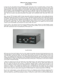
Ablasser. Some of the device vertices, net vertices and edges have been indicated as such.
device vertices
edges
Q2
D1
Q4
R3
1k
net vertices
Figure 2.3: A circuit expressed as a multiplace graph.
The method of detecting isomorphism is highly optimised. The graphs are reduced to adjacency
matrices, with each cell containing the number of connections between a particular node and spider.
The matrices for two isomorphic graphs A and B will have the same cells, but the order of the rows
and columns of the matrix for B will be a permutation of those for A. The algorithm attempts to
determine the mapping of vertices from A to B. If a total mapping exists, then the two graphs are
isomorphic.
Exhaustively testing each permutation would be very time-consuming, so Ablasser’s algorithm
labels the edges of the graphs with their type. This is simply their function in the original circuit. An
edge leading from a transistor might be labelled as “base” or “collector”. Adding this information
to the matrices simplifies the problem of mapping A to B.
Thus, Ablasser’s method is able to detect when two circuits have the same structure. This is
Chapter 2: Graph Theory
9
perhaps of some use to a student: students could draw part of a circuit, and then find a circuit
fragment that matched it in the database. However, Ablasser’s method would only find a match
if the two had identical structure. Thus, the student’s drawing could not feature any additional
components, even if those extra components were irrelevant to the circuit’s function. A tool based on
Ablasser’s method alone could be frustrating to a student, because of the requirement for exactness.
2.4.2
The Work of Spickelmier et. al., 1985
Spickelmier[18] suggests an alternative approach to that used by Ablasser. His work was also
intended for the verification of mask artwork against an original circuit.
Spickelmier notes that methods such as Ablasser’s depend on the properties of a circuit at a
local level. In Ablasser’s method, two components were matched by comparing their connections.
But this is not ideal, because it is quite possible that a large number of components may not be
distinguishable by this method. The only way to find the correct match would be to try them all,
which could be computationally expensive.
Spickelmier suggests that a rule-based system could be used to match the circuits. Rule-based
systems have applications in artificial intelligence: they make inferences based on some inputs and
a large list of logical rules. Spickelmier has applied an existing rule-based system to solve the
comparison problem (OPS5[8]), and written a program to generate the rules from the circuit. The
output produced is as follows:
First, each functional block (such as a logic gate) is described by a rule. The rule describes what
basic components (transistors, etc.) make up the functional block. Sometimes, a functional block
may take one of several forms - in this case, several rules may exist to match it.
Then, the program describes the entire circuit to be matched in rule form. The low-level
connections between basic components are listed: each link as a single rule.
This method of matching handles certain special cases very well. It is good at distinguishing
parts of the circuit that are very similar, such as memory cells in a RAM. It can also cope well
with permutations in the circuit. For instance, the inputs to an AND gate may be connected in
any order. But other comparison algorithms may insist that the order is exactly the same in both
circuits being compared.
The method also makes it easy to specify rules for functional isomorphism. Two circuits that
are functionally isomorphic have the same function, but may have entirely different structures.
However, the method is generally rather slow. It appears that it has poor time and storage
complexity, although the paper does not state the exact complexity, noting only that “subcircuits
with many elements increase the run time significantly”.
Spickelmier’s method is of particular interest because it could allow a circuit drawn by a student
to be matched with one in the database, even if the two had the same function but a different
structure. The method deals with what Spickelmier calls “transistor permutations” - where several
entirely different arrangements of transistors provide exactly the same function. This is common in
digital logic implemented on metal-oxide semiconductor (MOS) integrated circuits. It may also be
quite common in analogue circuits.
The main disadvantage of this method, in the context of this project, is that it requires a lot
of functional isomorphism rules to be specified beforehand. Unlike Ablasser’s method, and the
ones that will be seen later, it has to be “taught” the comparison rules. Additionally, a rule-based
inference system would be needed.
2.4.3
The Work of Takashima et. al., 1988
Takashima[23] describes a system that extends the ideas of Spickelmier and Ablasser. First, it
performs “reduction” on both circuits. Low-level components, such as transistors, are reduced
(where possible) to the logic gates they make up. This simplifies the network.
Next, the reduced circuits are compared by graph isomorphism. The algorithm used is from
another paper by Takashima[24], and is similar to Ablasser’s. There is one difference: components
that do not match are passed to a rule-based subsystem for comparison. This sub-system is able
10
A Graph Matching Search Algorithm for an Electronic Circuit Repository
to detect if the components have the same function, using a database of rules for functional isomorphism. Components that have different structures can still be matched if they have the same
function. The rule-based system is extensible.
Takashima explains that this allows his system to prove that two circuits are the same, even if
one of them has been optimised into an equivalent (but less complex) circuit. It is quite common
for a mask designer to make optimisations to the circuit during design, and these make it difficult
for systems such as Ablasser’s to show that the circuits are equivalent.
The techniques described by Takashima are said to be very fast, even on circuits with tens of
thousands of transistors. The slowest part of the process is the rule-based comparison. This was
found to be a serious problem by Spickelmier. However, Takashima has prevented this from being
a problem by doing as much work as possible by graph isomorphism and circuit reduction.
Like Spickelmier’s method, Takashima’s method has the potential to match circuits that have
the same function, but a different structure. This means that it could be a useful teaching aid.
Unlike Spickelmier’s system, however, rules are not needed for all types of matching. They are only
needed for cases where the graph isomorphism process cannot find a match. Fewer matching rules
would be needed.
2.4.4
Consolidation
The three papers that have been reviewed so far have described methods for comparing complete
circuits. This is not really what is needed: when students are searching for a circuit in a database,
they must not be limited to exact matches. However, interesting techniques have been described,
such as functional isomorphism. It may be possible to find circuits with a different structure but
the same function by making use of functional isomorphism algorithms.
Some research[12, 15] has been done into adapting the methods described earlier to find a
subcircuit within a larger circuit. This research will now be examined. As will be seen, it is directly
relevant to the problem to be solved in this project.
2.4.5
The Work of Luellau, 1984
A paper by Luellau[12] describes a program called “BLEX” - a program to find instances of a
functional block within a circuit. This is similar to the “reduction” technique applied by Takashima,
where a particular arrangement of transistors was identified as a particular logic gate. However,
while Takashima’s technique was hardwired with information about what to look for, Luellau’s
technique is general. The functional block may be any user-provided circuit of any size.
Luellau suggested that his program might be used to extract logic gates and larger components
from a circuit described at the transistor level. But this is only one use of the technique. It can
also be used to find a general subcircuit within a general circuit, and even to compare two circuits
of the same size.
The algorithm for subgraph isomorphism described by Luellau of particular interest. The algorithm described by Ablasser is used, but with an improvement: instead of labelling each vertex in
the circuit with the number of connections running to it, each vertex is labelled with a “signature”.
The signature identifies each vertex based on what is connected to it, and is rather like a hashing
function. If the connections to a vertex are different, the signature will be different. Thus, matching
vertices can be found simply by comparing their signatures. As will be explained in detail in Section
3.2.2, this leads to a very fast matching process.
Luellau’s method allows a subcircuit to be found within a circuit very quickly, and without the
need for any rules to be defined beforehand. Nothing is hardwired - the circuits are both general.
Luellau claims that the algorithm has typically near-linear time complexity with the majority of
circuits.
The method could be a significant part of the implementation of this project. It will allow
students to search for a part of a circuit they have drawn, or to search for the circuit they have
drawn as a part of a larger circuit.
Chapter 2: Graph Theory
2.4.6
11
The Work of Ohlrich, 1993
A paper by Ohlrich[15] describes improvements to Luellau’s work.
One significant improvement was made to signature generation. Signatures now describe more
of the circuit around a particular vertex: they are actually based on nearby signatures. As a result
of this, it is less probable that two or more vertices will share a signature: the signature is more
likely to identify a vertex uniquely. Ohlrich’s algorithm is therefore potentially faster.
2.5
The best direction to take
The research that has been examined has involved several different graph isomorphism algorithms,
which all make use of the special properties of circuits. Circuits are special types of graph. They can
be labelled in ways that make the matching process easier, as has been done by Ablasser, Luellau and
Ohlrich. Thus, circuit matching is not necessarily as difficult as the general subgraph isomorphism
problem, although (as will be proved in Section 3.2.4) this case of the subgraph isomorphism problem
is still NP-complete.
The papers that have been reviewed have made it clear that circuit matching is possible, and
efficient algorithms to do it already exist. It would certainly be possible to implement (for example)
Luellau’s algorithm and use it as the core of the search tool. It is possible to do three things, all of
which may be of use to a student learning about circuits:
• The student may draw a complete circuit, and then use the search tool to make a list of
circuit fragments in the database that are part of it: i.e. its subcircuits. Since the database
will include descriptions of those circuits, this will help to explain the operation of the student’s
circuit.
• The student may draw a fragment of a circuit, and ask in which of the database circuits it
can be found.
• Any circuit in the database that is isomorphic to the student’s circuit can be found, since any
subgraph isomorphism algorithm can also be used to detect graph isomorphism.
The first of these is likely to be the most useful. One can imagine that, for user-friendliness, the
list of subcircuits might be restricted to those involving certain user-selected components. Figure
2.4 shows a possible sequence of events.
Darlington Pair
Arranging two transistors in
this way gives a much higher
current gain than either transistor
alone. The total current gain is
equal to the product of the current
gain of each transistor.
(1)
(2)
(3)
Figure 2.4: An example of a search. The student draws a Darlington pair, as part of a larger circuit
(1). Wishing to learn about this part of the circuit, the student clicks on one of the transistors in the
pair, which becomes highlighted (2). A database search then reveals all of the database circuits that
are a subcircuit of the entire circuit, and include the selected transistor with the same connections.
There is only one such circuit: the Darlington pair. This result is displayed (3).
With the addition of an additional procedure to compare the component value associated with
each device, additional types of search will become possible. Some devices have values associated
with them, such as “resistance” in the case of a resistor, and it will become possible to insist that
12
A Graph Matching Search Algorithm for an Electronic Circuit Repository
any matches that are found must have exactly the same device values. It will also be possible to
assign a score to each match that is found, according to how closely the device values matched.
However, the algorithms that have been looked at so far are not necessarily the best way to
achieve this. To search a database of m circuits using any of the algorithms would take at least mn
operations, if each circuit contained at least n components. This is not ideal. But not all search
methods need to take this long.
If a program was searching a dictionary for a word, it could search through all possible words
until the word was found. This would be a linear time operation. It would be better to sort the
dictionary in alphabetical order, because this would allow a binary search to be used. This would
complete faster: in O(log n) time for n words. It would be even better to store the words in a hash
table. Then it would be possible to find a word in the dictionary in constant O(1) time. It should
not be a surprise, then, that this last technique is the one that is used in spell checking software.
Related techniques can be applied to circuit matching. When this project was started, it was not
clear what they would involve, and (to date) no researchers appear to have addressed this problem.
However, research undertaken by the author has led to the development of a database structure
that allows the number of circuits that need to be examined to be minimised. This structure will
be discussed in a later chapter.
Chapter 3
Evaluation of Existing Algorithms
In the previous chapter, it was stated that Luellau’s algorithm could be used as the core of the
search tool. Ohlrich’s algorithm could also be used. These are not necessarily the most efficient
algorithms for a search within a database: but implementing them helps the author to gain useful
insight into how they operate. In addition, the implementations form the basis for the search tool
and the test tools that were developed for it.
3.1
Groundwork
No matter how circuit comparison is carried out, the circuit structure that is used will come from a
circuit description in SPICE[30] format. All of the algorithms will need to be able to interpret the
SPICE format, which will now be examined.
3.1.1
The SPICE File Format
SPICE files are human-readable text files, in which each line is called a “card”. There are three types,
which can be divided into “control” cards (containing commands), “element” cards (describing
electronic devices), and comment cards.
The circuit illustrated in Figure 3.1 is described by the SPICE file in Figure 3.2.
7
R1
4k
R2
1k6
2
R4
130
6
Q3
4
5
1
Q1
Q2
3
D1
8
Q4
10
R3
1k
0
Figure 3.1: An inverter circuit.
13
14
1
2
3
4
5
6
7
8
9
10
11
12
13
14
15
16
17
18
19
A Graph Matching Search Algorithm for an Electronic Circuit Repository
Inverter (7404)
.WIDTH IN=72 OUT=80
* Input: 1 Output: 5 VCC: 7
.SUBCKT INVERTER 1 5 7
Q1 3 2 1 N
Q2 4 3 10 N
Q3 6 4 5 N
Q4 8 10 0 N
D1 5 8 DIODEM
R1 7 2 4K
R2 4 7 1.6K
R3 10 0 1K
R4 6 7 130
.ENDS INVERTER
.MODEL DIODEM D
.MODEL N NPN(BF=75 RB=100 CJE=1PF CJC=3PF)
X1 100 200 300 INVERTER
VCC 300 0 DC 5
.END
Figure 3.2: The SPICE circuit description for the circuit illustrated in Figure 3.1.
In Figure 3.2, the lines beginning Q, R, D and X describe four types of electronic device: they
are element cards. The lines beginning * are comments, as is the first line (the “title”). The lines
beginning with a . are control cards. Many of these can be safely ignored: giving hints to the
SPICE interpreter that do not affect the structure of the circuit. The ones that cannot be ignored
are the .MODEL, .SUBCKT, and .END control cards.
Most element cards translate directly to device vertices. The only exception is the SPICE
subcircuit element, denoted by the .SUBCKT card. Subcircuit elements are analogous to procedure
calls. Each subcircuit element is replaced with all the elements that make up the subcircuit. Here,
the subcircuit element X1, on line 17, is replaced with all the elements in the INVERTER subcircuit
(lines 5 to 13). As can be seen in Figure 3.1, no trace of X1 remains when the complete circuit is
drawn out.
The .MODEL control card describes the parameters used to model devices such as diodes and
transistors. The parameters are largely irrelevant to this project. However, in the case of transistor
models, the type of transistor is very important. SPICE supports many different transistor types:
NPN, PNP, and two types of JFET and MOSFET. It is essential to take the type of a transistor
into account during circuit matching, because each type has entirely different behaviour.
3.1.2
Interpreter Design Decisions
The SPICE interpreter had to be easily adaptable for use by a wide variety of algorithms: in
particular, those of Luellau and Ohlrich.
The algorithms could operate directly on the information in the SPICE file, comparing two
circuits in SPICE format directly. However, this would lead to a very poor design in two ways.
First, the implementations of the algorithms would have to include code to interpret the SPICE
file, and this would obscure the operation of the algorithm itself. In effect, the source would be
filled with code that had no relevance whatsoever to circuit comparison. Second, the code to read
SPICE files would be replicated between all algorithms that made use of it. Any bugs in that code
would exist in at least two places, and it would be difficult to make any extensions to it.
It is far better to have a layer of abstraction between the SPICE interpreter and all comparison
algorithms. This layer would consist of a circuit description format that is common to all algorithms and the interpreter, and would be simple enough to allow immediate access to all relevant
information.
It is this approach that was chosen because of the clear advantages it brings. Comparison code
can be more readable, and all code involved with reading SPICE files is in one place. It also brings
the advantage that circuits can be stored on disk in other formats, which proved to be very useful
once a serialisation feature was added to allow circuits to be stored within the database.
Chapter 3: Evaluation of Existing Algorithms
3.1.3
15
A choice of languages
Since the Book Emulator is written in C, the programming languages available for implementing
the search tool are C and its superset language C++.
The C++ language was chosen for three reasons. Firstly, the language supports inheritance. So
an algorithm can be made to use a generic interpreter class just by inheriting it. This provides a
framework for the abstraction layer between the interpreter and the algorithm.
Secondly, the language supports a library of abstract data types known as STL: the Standard
Template Library[14]. These types, which include sets, hashes and binary heaps, make it easy to
implement any algorithm efficiently and correctly. They were heavily used in the implementation of
the search tool. Finally, the language includes several features that make it easier to write correct
code, none of which are available in C.
C++ is strongly typed, so bugs are not normally introduced by type conversions. A reference
type is available which provides a safe alternative to pointers in many situations. Unlike pointers,
reference types are never “null” and can never point to unused or unavailable memory. There is
also no need to allocate or free reference types: memory allocation for these types is managed
automatically, so there is no chance of a memory leak developing.
More subjectively, the object-oriented nature of C++ leads to better software engineering practices. It encourages the programmer to adopt an object-oriented mindset and think carefully about
the structure of the program. Of course, it is still possible to write poorly designed programs in
C++, but the author has found that using C++ allows him to write better code. The “correct
way” to achieve something is usually apparent from the object-oriented structure.
A C++ class called SPICE Interpreter was written, capable of reading a SPICE circuit description, and building data structures to represent the circuit. These structures can be used directly by
circuit matching algorithms.
As stated in the previous chapter, circuits are considered to be bipartite graphs consisting of
device vertices and net vertices. Device vertices represent devices such as transistors and resistors.
Net vertices represent any place where two or more wires are connected. This is the naming scheme
used by Ohlrich[15], and it is used because it is considered to be less confusing than the equivalent
naming scheme used by Ablasser[1] and Luellau[12].
The representation of a circuit used by Ablasser, Ohlrich and Luellau allows a device to have
more than two connections, unlike the representation suggested in Figure 1.1. Additionally, when
n devices are connected to a single point, only n connections are needed to that point, instead of
the O(n2 ) connections that would be required using the Figure 1.1 representation.
3.1.4
Implementing the SPICE Interpreter
SPICE Interpreter was written as a single C++ class. It translates a circuit description in the
SPICE format, as described in Section 3.1.1, into a variety of C++ data structures.
The constructor of the class is given a file name as a parameter. It reads the file, expanding all
SPICE subcircuits so that the entire circuit is “flattened” into a single graph. The graph consists
of device and net vertices. The data structures that are produced are as follows:
• A Device Vertex object is produced for each device. The object includes information about
the device (type and model number) and a list of connections.
• A Net Vertex object is produced for each net vertex (connection point). The object includes
a list of connections.
• Each connection is described by a Net Vertex Connection structure.
• Three “master lists” are produced, containing all net vertices, device vertices, and connections
respectively. These make it easy to apply an operation to every vertex or edge, and to destroy
the data structures when the SPICE Interpreter object is deleted.
16
A Graph Matching Search Algorithm for an Electronic Circuit Repository
Using these data structures, it is possible to traverse the entire graph starting at a single device,
net vertex or connection. All of the connections can be followed in constant time, so navigating
between n vertices requires O(n) operations.
Open and Closed Vertexes
At a later stage in the project, it became apparent that it would be necessary to draw a distinction
between vertices that are open and those that are closed. This terminology, which is used in several
papers[12, 15], is used to distinguish between the vertices that can act as extension points for a
circuit and the vertices that cannot.
An open vertex is a point in a circuit that may have anything added to it by a supercircuit of
that circuit. A closed vertex may not have anything added to it by any supercircuit. Figure 3.3
illustrates this with a simple example.
Key
Open Net Vertex
Closed Net Vertex
x
(a)
(b)
(c)
Figure 3.3: All of the vertices in (a) are closed. (c) cannot be a supercircuit of (a) because (c)
makes an extension to (a) that is not permitted, since the extension is made to a closed vertex.
However, one vertex in (b) is open (marked as x). (c) is a supercircuit of (b), because it makes an
extension to (b) at the open vertex x.
It is very important that the comparison algorithm recognises the difference between open and
closed vertices, because some apparent extensions to a circuit are misleading. They are not extensions to the original circuit or improvements to it: they are entirely different circuits in which the
existence of the original circuit is merely a coincidence.
There is no way to represent open and closed vertices in SPICE. One method would involve the
addition of specially formatted comments to every SPICE file to indicate which vertices should be
considered to be open (or closed). In this way, the SPICE files would still be readable by SPICE,
but the extra information would be available to the circuit repository software.
However, a more elegant method would make use of the subcircuit feature that is already built
into SPICE. A SPICE subcircuit incorporates internal vertices that are only accessible within the
subcircuit. It is natural to assume that these internal vertices should be closed: after all, they are
not reachable from components outside the subcircuit. Additionally, any extension of a particular
circuit would have to have the same SPICE subcircuits with it. So, any vertex within a SPICE
subcircuit can be assumed to be closed, and all other vertices can be assumed to be open. This
method appears to be an ideal match for the hierarchical way that SPICE circuits are designed.
Power Supply Devices
SPICE includes some special devices to represent voltage and current sources. It was decided that
these devices should be omitted from the graph representation because they provide no reliable
information about the structure of the circuit. These sources do allow certain vertices to be marked
as “power sources”, but this is not useful for matching, since there are many equivalent ways to
connect a power source to a particular circuit. For example, a +5V voltage source connected between
vertices 1 and 0 would be equivalent to a -5V voltage source connected between vertices 0 and 1.
The basic problem is that if vertices are marked as “power sources”, or marked as special in
any way, then the only possible matches for those vertices will be ones in which those vertices are
marked in the same way. The matching will no longer be merely structural, it will be based upon
vertex markings. As a result, no voltage or current sources are included in the graph representation.
Chapter 3: Evaluation of Existing Algorithms
3.2
17
Luellau’s algorithm
Luellau’s algorithm[12] was described in a paper about a computer program called “BLEX”. BLEX
is able to take a circuit described at the transistor level and find “blocks” from it, such as logic gates
and flip-flops. This “block extraction” process is circuit matching, because each block is described
by a circuit fragment, and BLEX must find all instances of every block in the overall circuit.
Neither binaries nor source code for BLEX are available, but there was enough information in
the paper to implement it from scratch.
3.2.1
Implementation
Having written the SPICE Interpreter class, it was straightforward to extend it. A second class,
Luellau Circuit, was written. This added a Compare To function, which compares one circuit with
another using Luellau’s algorithm. This returns TRUE if one circuit is an isomorphic subgraph of
the other, and FALSE otherwise.
3.2.2
Operation of the Algorithm
Luellau’s algorithm works in three phases. The first phase finds suitable starting points within the
smaller of the two circuits, by attempting to find a net or device vertex with a maximal number of
unique edges. A unique edge of a vertex is one that can be distinguished from all the other edges,
because it is connected to a type of device that no other edges are connected to.
Once a suitable starting point is found, the set of vertices that are equivalent to it in the larger
circuit are found. One is selected as a match. This is the non-deterministic phase of the algorithm,
because there may be more than one possible equivalent vertex. The algorithm may pick the wrong
one and be forced to backtrack.
The third phase of the algorithm is deterministic. It is a gradual process in which items in
the smaller graph are matched to items in the larger graph. Two items are only matched if the
algorithm can be certain that they are equivalent. Provided that the correct match was made in
the second phase, the matches made here will all be correct.
Figure 3.4 illustrates this phase. In the example shown, eight iterations of the third phase are
required to match the vertices of the subcircuit to those of the circuit. The borders between the
vertices that are labelled in one iteration and those that are labelled in the next are indicated by
dotted lines. The set of matched vertices grows until all subcircuit vertices have been matched.
8
4 6
7
R1
4k
R2
1k6
5
1
6
9
Q1
Q3
Q2
unmatched
7
R1
4k
4
10
D3
2
2
3
1
R2
1k6
1
Q6
4
Q2
3
R4
130
5
4
5
2
3
Dk
1
8
Q4
10
3
5
2
3
R3
1k
4
6
6
6
Q3
2
R3
1k
D2
8
7
Q4
Q5
8
7
7
5
3
2
D1
R4
130
8
0
4
8
7
6
5
0
Figure 3.4: An example of Luellau’s algorithm in action, with the vertices that are matched at
each iteration separated by dotted lines. The circuit on the right (an inverter) is a subcircuit of the
circuit on the left (a NAND gate). In the first iteration (marked 1), Dk is matched to D3. Then,
during the next seven iterations, net vertices and device vertices are matched up.
The third phase may fail, in which case the algorithm will return to the second phase and make
18
A Graph Matching Search Algorithm for an Electronic Circuit Repository
a different choice. If no choices remain, then the circuits do not match and the matching function
will return FALSE.
Sometimes the algorithm will take more than one iteration to match everything. If the third
phase completes, but unmatched vertices remain in the smaller circuit, then the matches that have
been made are finalised and the algorithm repeats from phase one.
3.2.3
Details of the Algorithm
The algorithm matches edges, net vertices and device vertices by using a property of prime numbers.
Any positive integer can be expressed as the product of prime factors: the result of multiplying one
or more prime numbers together. The set of prime factors for a particular number is unique. For
example, the number 1980 is the product of the following prime factors:
2 2 3 3 5 11
There is no other multiset of prime numbers that multiply together to give 1980. This property is
used by Luellau’s algorithm. Every edge is assigned a weight, which is a prime number. Assignments
are made according to the type of device that it is connected to, and according to which pin the
edge is linked to. Table 3.1 lists the assignments used by Luellau, which are easily extended with
new weights for the JFET and MOSFET components supported by SPICE.
Device Type
Resistor
NPN Transistor
PNP Transistor
Diode
Capacitor
Pin Type
Base
Collector
Emitter
Base
Collector
Emitter
Cathode
Anode
Edge Weight
2
13
11
3
17
5
7
19
23
29
Table 3.1: Luellau’s Algorithm: Edge Weights
Every vertex is also assigned a weight: the product of all the edge weights that are directly
connected to it. Because any product of prime factors uniquely identifies the prime factors that it
is composed of, the weight of a vertex uniquely identifies the edges connected to the vertex.
It is easy to tell when two vertices are not equivalent. Device vertices are not equivalent if the
weights are not the same: a simple check for equality is sufficient to see that no match can exist.
In the case of net vertices, the test is moderately more complex. Net vertices may be open or
closed, as described in Section 3.1.4. A closed net vertex in the smaller of the two circuits can only
be equivalent to a net vertex in the larger circuit if it has an identical set of edges connected to it.
So closed net vertices can be compared to possible matches in the same way as device vertices: if
the weights are exactly the same, then the two vertices are equivalent.
Open net vertices are compared using another property of prime factors. Because an open net
vertex in the smaller circuit must have a subset of the edges of its equivalent vertex in the larger
circuit, the weight of the vertex in the larger circuit must be divisible by the weight of the vertex in
the smaller circuit. The same edges have to be present in both weights, although extra edges may
be present in the larger circuit. The division check ensures that the edges that must be present are
indeed present.
In general, comparing the contents of two multisets to see if one multiset is a subset of the other
would take O(n) time: and even more than this if the multisets are unsorted. In this specific case,
the properties of prime factors allow the same comparison operation to be done in O(1) time.
Chapter 3: Evaluation of Existing Algorithms
19
On a related note, the algorithm requires that a two dimensional matrix of edge weights be
maintained for each circuit. The size of this matrix is potentially very large, and as Luellau notes
in the paper, “approximately 99.75% of its elements are zero”. If the matrix were represented as an
array, it would be possible to find or change the value of an element in constant time. However, the
matrix would require a large amount of space, to the order of the product the number of devices
and the number of connection points.
Another way to represent the matrix but preserve constant time access is to make use of a hash
table. The hashing function takes both dimensions of the matrix as its input. The disadvantage
of this technique is that operations on the matrix as a whole, such as summing a row, are very
expensive. Fortunately, such operations are not necessary to implement Luellau’s algorithm.
3.2.4
Time complexity of the Algorithm
The worst-case time complexity of Luellau’s algorithm is exponential. Proof:
1. Subgraph isomorphism is in N P [10].
2. There is no known algorithm that can solve any problem in N P in polynomial time. All
problems known to be in N P require O(en ) operations to be solved, in the general case. Any
algorithm that could solve such a problem in polynomial time would constitute proof that
P = NP.
3. It is possible to translate any general subgraph isomorphism problem X into a circuit comparison problem Y that can be solved by Luellau’s algorithm.
• Every node in X must become a net vertex in Y .
• Every edge in X must become a resistor (or any other component with two unordered
connections). So an edge connecting graph nodes a and b becomes a resistor linking net
vertices a and b.
This translation can be done in linear time.
4. If Luellau’s algorithm always completed in polynomial time, then it would be possible to use
it to solve the general subgraph isomorphism problem in polynomial time, by translating a
general instance of the problem into a circuit (3). Since the problem is in N P (1), this would
constitute proof that P = N P (2).
So, provided that P 6= N P , Luellau’s algorithm will take exponential time to complete in the
worst case. However, experimentation with the algorithm suggests that the worst case is most
unlikely to occur in any real circuit. This was found by the authors of the algorithm, who stated
that “the runtime increases almost linearly with the number of devices”.
This is because restrictions can be placed on the types of match that are possible. For example,
there are two types of vertex, which can only connect directly to vertices of the other type. And
one type of vertex (device vertices) has a defined number of external connections and can only
be matched to a particular sort of device. This information simplifies the subgraph isomorphism
problem and reduces the amount of time it takes to run.
It is always possible to construct a circuit that provides no additional information, such as the
one described in part 3 of the above proof, which had only one type of component. But a typical
circuit will contain a wide range of different components, interconnected in distinctive ways, and
this will be far easier to match.
3.2.5
Testing the implementation
A simple way to test the implementation of the algorithm is to use the example circuits described
in the paper. The paper uses these circuits to explain what the algorithm should do at each stage,
and describe what it should output. A debugging build of the Luellau Circuit class was used
which printed out information about every decision made. The circuits under test were taken from
20
A Graph Matching Search Algorithm for an Electronic Circuit Repository
the paper. The output matched the description given in the paper, and the match that was found
was identical. This provided a good indication that the implementation was correct.
Later tests were performed on a small corpus of circuits from a course in digital circuit design
featured in the Book Emulator[3]. These circuits were primarily ones from the 74 series of integrated
circuits. For example, a 7404 inverter is a subcircuit of a 7400 NAND gate, and Luellau’s algorithm
was able to detect this. It was also able to print out the correct translation of 7404 vertices to 7400
vertices.
Finally, some stress tests were performed using circuits that were intended to approach worst
case behaviour. This was done by choosing circuits that maximise the non-deterministic portion of
the algorithm: ones where all the vertices are indistinguishable from each other. Matches based on
these circuits were slow, but completed correctly.
3.2.6
Disadvantages of Luellau’s algorithm
One disadvantage of Luellau’s algorithm comes from its use of products of prime factors to label
vertices. While this technique does allow constant-time comparisons of vertices in the two circuits,
the number of edges that can be connected to any particular vertex is limited by the storage space
available for the resulting product.
A 32-bit “unsigned” integer can take any value from 0 to 232 − 1. Suppose we wish to store
x instances of a prime number a in this integer. The product of prime factors will be ax . The
maximum possible value of x is bounded by ax ≤ 232 − 1. Any larger values of ax cannot be stored.
Even if a is the smallest prime number (two), the maximum number of instances of a that can
be stored in the integer is 31. If a is the largest prime number in Luellau’s numbering scheme (Table
3.1), which is 29, then x must be less than seven1 . So, in the worst case, only 6 devices can be
connected to a single point in the circuit.
This limit is rarely reached in a small analogue circuit. Most devices are only connected to a
few other devices. But exceptions occur all the time in large circuits: consider how many devices
are connected directly to ground.
The problem cannot be offset simply by using larger integers. Using 64-bit integers will still
bring a worst-case limit of just 13 devices. It is possible to use variable-precision integers, which
can store any number that will fit in the memory space of the computer. But operations on these
numbers are not constant time, and so the advantage of using prime factors has been lost.
However, the problem can often be ignored. Luellau certainly makes no mention of it in the
paper. This is probably because the labels generated by the prime factor method still identify
vertices (almost) uniquely, even if a multiplication overflow occurs during calculations. Only one
property is lost due to overflow. If net vertex y is equivalent to open net vertex x, with some extra
components, then y is divisible by x. But if an overflow occurred during the calculation of y, then
this does not hold: not least because y is now less than x. Because this property is not always
required to hold, the algorithm may perform as expected even if an overflow occurs. Then again, it
may not. A subtle bug has been introduced.
A second disadvantage of Luellau’s algorithm was found only after extensive testing. It is a flaw
in the algorithm that occurs only in rare cases, but is a potentially serious problem.
Luellau’s algorithm needs to find a starting point to begin analysis of a circuit. The starting
point will be the vertex with the maximum number of unique edges: edges with a weight that does
not appear elsewhere in the circuit. Unfortunately, some circuits have no such edges. A very simple
example of such a circuit is shown in Figure 3.5.
In this circuit, there are two edges (between a and b, and b and c), but the edges cannot be
distinguished. As a result, Luellau’s algorithm cannot find a point in the circuit to start matching,
and always fails. Luellau’s paper does not define what should be done in this situation. The
algorithm can easily be modified to report an “inconclusive” result if this situation arises, but this
is not very useful in a search tool that is supposed to find exact instances of subgraph isomorphism.
1
To find the maximum value of x, let ax = 232 − 1. Taking the logarithm of both sides, x log a = log (232 − 1).
(232 −1)
(232 −1)
Then, x = log log
= loglog
≈ 22.18
≈ 6.58. Thus, in practice, x ≤ 6.
a
29
3.367
Chapter 3: Evaluation of Existing Algorithms
a
b
21
c
R1
1k
Figure 3.5: Luellau’s algorithm cannot find any supercircuit for this circuit, because none of the
three vertices (marked a, b, and c) have unique edges.
3.3
Ohlrich’s algorithm
Ohlrich’s algorithm[15] is the main part of a system called SubGemini, which is able to find instances
of a circuit within another circuit. Unlike the original implementation of Luellau’s algorithm, the
SubGemini source code is available, and staff at the University of Washington were kind enough to
send a copy to the author.
The source code provides two things. First, it is a useful reference implementation that can be
used to clarify details of the algorithm that may not be clear from the paper, and guide any other
implementation. Second, it is able to solve the entire problem by itself, so it is possible to analyse
Ohlrich’s algorithm without any additional implementation.
3.3.1
Reimplement or not?
The availability of SubGemini gave the author a choice: should the algorithm be reimplemented, or
should the existing version be used? Reusing the existing version would give two advantages. The
implementation was known to be correct, and less work would be required. In fact, it would only
be necessary to compile SubGemini on a modern computer, and find a way to make it read circuits
in SPICE format. Neither of these were expected to be difficult.
However, there are other disadvantages of this code reuse. Firstly, it is unscientific to compare
two algorithms unless the environments they operate in are as similar as possible. SubGemini is
not only an implementation of Ohlrich’s algorithm: it contains procedures to read data in from files
and output answers. It would be unfair to compare the SubGemini program directly to the Luellau
program written in Section 3.2, because they have different input and output procedures.
Secondly, it is stated on a University of Washington website that “the SubGemini program exists
only as a prototype”[5]. Since it was never considered to be finished, the reliability of the code is
questionable: particularly as this project would apply SubGemini in a way that it was not intended
to be used, which might unearth bugs that were not found by the original authors.
3.3.2
Implementation
A new class called Ohlrich Circuit was written. This inherited from SPICE Interpreter, adding
a Compare To function (just like the Luellau Circuit class).
3.3.3
Differences between the Algorithms
Ohlrich’s algorithm is very similar to Luellau’s algorithm. It operates in two phases: during the
first, a “key” vertex is chosen from the smaller graph, and a list of possible matches for that vertex
is found in the larger graph. This list is called the “candidate vector”. This is done by labelling
every vertex in both circuits with a label that identifies its type and the number of connections to
it.
In the second phase, the algorithm makes a tentative match between the key vertex and one of
the vertices in the candidate vector. This match is used as a starting point for a gradual match of
the entire circuit. The gradual matching process is very similar to the process used by Luellau’s
algorithm, which was illustrated in Figure 3.4.
However, a number of improvements have been made. First, the method by which the starting
point is found is vastly improved. The choice of a good starting point is critical to both algorithms.
22
A Graph Matching Search Algorithm for an Electronic Circuit Repository
Both Luellau and Ohlrich note that the running time of the gradual matching process is far greater
than that of the first phase - but the time spent in this phase depends on the choice of key vertex.
For example, in the circuit in Figure 3.6, there are four transistors, four resistors and one diode.
If an algorithm is searching for a subcircuit of Figure 3.6, a diode would be an excellent choice of
key vertex in the subcircuit, because it can only be matched to D1.
7
R1
4k
R2
1k6
2
R4
130
6
Q3
4
5
1
Q1
Q2
3
D1
8
Q4
10
R3
1k
0
Figure 3.6: An inverter circuit, reproduced from page 13.
Luellau’s algorithm always chooses a starting vertex with a maximal number of unique edges.
When the algorithm compares Figure 3.6 with an identical circuit, it chooses Q4 as the key vertex.
This is a very poor choice, because there are three other transistors that Q4 could be matched to.
The gradual matching process is run three times until the correct match is made.
However, Ohlrich’s algorithm correctly selects D1, because it chooses a key vertex with the
intention of minimising the size of the candidate vector. As a result, when Ohlrich’s algorithm
compares Figure 3.6 with itself, the gradual matching process is run only once.
Ohlrich’s algorithm consistently chooses a starting point that results in a candidate vector that is
the same length or shorter than that chosen by Luellau’s algorithm. This can be shown by a simple
experiment based upon the corpus of circuits that was mentioned earlier. When two circuits are
selected from the corpus and compared, the size of the candidate vector found by Luellau’s algorithm
is never less than the size of the candidate vector found by Ohlrich’s algorithm, regardless of the
circuits that are chosen.
To quote Ohlrich’s paper, “the running time remains reasonable...because Phase I is usually able
to find the right [vertex]”. Selecting the best candidate vector is essential for efficient matching.
The fact that Ohlrich’s algorithm does not depend on unique edges also allows it to handle
circuits in which no unique edges exist, such as Figure 3.5. This is a second advantage over Luellau’s
algorithm.
A third advantage of Ohlrich’s algorithm comes from the fact that the labels assigned to vertices
are not fixed. Vertexes are relabelled during the matching process under two circumstances:
• When two vertices are matched together, they are both assigned a unique label that never
changes.
• Whenever an unmatched vertex V is next to one or more matched vertices, it is relabelled by a
procedure that takes into account the current label of V and the labels of all the neighbouring
matched vertices.
By doing this, Ohlrich’s algorithm makes use of the information that it has gained about the
circuit during earlier matches. This allows it to distinguish between vertices in circumstances where
Luellau’s algorithm could not.
Chapter 3: Evaluation of Existing Algorithms
23
A fourth advantage of Ohlrich’s algorithm is that it does not use prime factors to label vertices
at any time. In Luellau’s algorithm, prime factors were used because they always uniquely identify
a particular set of connections, and can also be used to detect if one set of connections is a subset of
another. Ohlrich’s algorithm never needs to check for the second condition, because it handles open
vertices differently to Luellau’s algorithm. So there is no particular reason to use prime factors,
provided that labels that uniquely identify a set of connections can still be generated. The result is
that arithmetic overflow presents no problems to Ohlrich’s algorithm, and the algorithm can work
with arbitrarily large numbers of connections to a single vertex.
Finally, Ohlrich’s algorithm returns more information than just “yes” or “no”. It is able to
indicate the number of instances of subgraph isomorphism that were found. If the smaller circuit
can be fitted into the larger circuit in two different ways, then the algorithm will be able to indicate
this.
3.3.4
Testing the implementation
All of the tests that were performed on the Luellau Circuit class were repeated for Ohlrich Circuit. The same test tool could be reused, since both classes present the same interface to other
parts of a program. It was only necessary to substitute Ohlrich for Luellau in the test procedure.
In addition, some new tests were possible. The two algorithms should produce the same answer
when asked to compare any two circuits, so a second test tool was written to take advantage of this.
The tool worked from a corpus of 27 circuits, most of which were extracted directly from the Book
Emulator[3] using a tool developed by Keffin Barnaby as part of his project[2]. Other circuits were
entered by hand.
The test tool selected every possible pair of circuits from the corpus, and ran the two algorithms
on them. The results of the comparison given by both algorithms had to be the same: if it didn’t,
the test halted with an error. And if a circuit was being compared to itself (an “autocomparison”),
then both algorithms had to report a match.
During testing, it was found that some of the circuits in the corpus caused Luellau’s algorithm to
terminate with an error, due to the unique edges problem described in Section 3.2.6. The algorithm
had not been able to find any unique edges, so it was not able to carry out any comparison. The
results of these tests had to be discarded: however, only a minority of tests ended in this way.
The implementation was also tested by a “random stress test” called breakdown.cc. In this test,
a circuit was generated at random by a test tool and stored in SPICE format. The circuit contained
a random (non-zero) number of components, connected together randomly. A supercircuit of that
circuit was then constructed by adding a random number of additional components to it. The test
tool then ran the following tests using Ohlrich’s algorithm:
• The smaller circuit is a subcircuit of itself.
• The larger circuit is a subcircuit of itself.
• The smaller circuit is a subcircuit of the larger one.
• The larger circuit is not a subcircuit of the smaller one.
Since the circuits are generated, the correspondence between each subcircuit vertex and each
supercircuit vertex is always precisely known, and this correspondence was checked by the test tool
to ensure that Ohlrich’s algorithm found the exact match.
The test tool examined huge numbers of these circuits. It was left running for a day, and it
tested 115,548 different circuits. All of the checks listed above passed for every circuit.
Of course, this test only really shows that Ohlrich’s algorithm can find positive examples: places
where the smaller circuit is a subcircuit of the larger one. The fourth check is intended to find a
negative example, but its value is limited. The larger circuit cannot possibly be a subcircuit of the
smaller one, since it has more components. However, the other tests show that Ohlrich’s algorithm
can identify negative examples correctly.
24
A Graph Matching Search Algorithm for an Electronic Circuit Repository
The test also involved only randomly generated circuits. These circuits are generally electronic
gibberish. The reader may question how a test using only this type of circuit could have any
relevance to an algorithm that, in practice, will be used on real circuits. The answer is twofold:
first, random circuits provide pathological examples of unstructured circuits that are difficult to
match. Second, any useful circuit will be generated by a random process given sufficient time. It is
almost certain that some practical circuits were generated and tested during the test run.
3.4
Conclusions
At this point, it is clear that Ohlrich’s algorithm is superior to Luellau’s. Three of the most
important advantages are:
• Luellau’s algorithm cannot handle every circuit. For example, it cannot find supercircuits of
Figure 3.5. Ohlrich’s algorithm appears to be able to handle all circuits, according to the
testing that has been performed by the author and the claims of the algorithm’s designers.
• Ohlrich’s algorithm consistently chooses either the same starting point as Luellau’s algorithm,
or a better one, resulting in a smaller candidate vector.
• Ohlrich’s algorithm is not subject to any limitation on the number of vertices that may be
connected together, whereas the reliance on prime factors in Luellau’s algorithm causes a
problem when large numbers of vertices are connected.
The search tool that was implemented is based upon Ohlrich’s algorithm. However, the algorithm
cannot be used by itself. Ohlrich’s algorithm only compares two circuits: and the search tool needed
to match a single circuit against a large number of circuits to find the best matches.
In addition, Ohlrich’s algorithm has no support for comparing the values of devices. This had
to be implemented separately, and the discussion of the implementation can be found in Chapter 6.
Chapter 4
Improvements to Ohlrich’s
comparison algorithm
The project aims to produce a search tool that can compare a circuit provided by a user to a large
number of circuits stored in a database.
In general, there are two ways to optimise any search process. First, there is optimisation of
the method by which candidates for matching are chosen, which is called the “search method”.
Second, there is optimisation of the comparison process that is used: the “comparison method”.
The comparison method acts on two items at a time, and indicates the relationship between them.
Consider the example of searching a dictionary for a word. Here, a poor search method would
involve examining every word until the one being searched for was reached, requiring O(n) comparisons for a dictionary of size n. The optimum search method is a binary search, because the words
in the dictionary are sorted into alphabetical order. O(log n) comparisons are required to find a
word, and the optimum comparison method compares words one letter at a time: only advancing
to the next letter if the current letter is the same in both words.
In the case of circuit comparison, Ohlrich’s algorithm provides the comparison method. The
search method is yet to be defined, but it cannot be the naı̈ve method of scanning every circuit in
turn, just as a dictionary search should avoid examining every word until the correct one was found.
So one way to improve the speed of searches is to improve the speed of Ohlrich’s algorithm.
The algorithm appears to be highly optimised. However, one area for improvement lies in the data
structures that it uses.
4.1
Hash tables or red-black trees?
The paper[15] does not recommend any particular data structures for use in the implementation of
the algorithm. However, the original implementation of the algorithm (obtained courtesy of staff
at the University of Washington) does provide a guide.
Practically all the structures that are present in the original implementation are open hash
tables, which are excellent structures to be used whenever random access is required to some data
by some type of key. In Ohlrich’s algorithm, the data is a list of vertices, and the key is the label
assigned to all of those vertices.
The choice of hash tables is a mistake. Ohlrich’s algorithm regularly requires all vertices to be
examined by a relabelling process, and in order to achieve this, the algorithm iterates through every
member of the hash table. Hash tables are not efficient when they are used in this fashion, because
the time complexity of the operation is at least linear in the size of the hash table, and not linear
in the number of items in the table as might be expected. The size of the table may be much larger
than the number of items in it - indeed, it is usually a good idea to ensure that a hash table is as
large as reasonably possible.
A comment that appears in hash.c indicates that the developers of the original implementation
changed their minds about the use of hash tables:
This whole hash table stuff was probably a mistake in the false assumption that there
25
26
A Graph Matching Search Algorithm for an Electronic Circuit Repository
were going to be a lot of partitions. Since there are usually not, we can just use linked
lists or something like that.
The author of this comment is correct - the use of a hash table to store vertex data was a mistake.
However, the solution proposed (“linked lists”) is no better, because the algorithm requires more
than simple iteration through each set of vertex data. It also requires random access. There are
some operations which require vertices with particular labels to be found, such as “test equivalence
classes”, in which the labels present in the smaller circuit are checked against those in the larger
circuit.
A red-black tree[13] is a much better choice of data structure. A red-black tree is a balanced
binary tree with the property that the search for a node will take O(log n) operations, if there are
n nodes in the tree. Deletions and insertions of a single node also take O(log n) operations. And
iteration through all n nodes can be performed in O(n) time. Red-black trees can replace hash
tables in Ohlrich’s algorithm to good effect.
Red-black trees are slightly slower than hash tables for searches, insertions and deletions. Hash
tables can carry out these operations in constant time if they are large enough, whereas red-black
trees require O(log n) time. Despite this, red-black trees have much higher efficiency for operations
involving iterating through every item. Those operations are O(n).
A second advantage of red-black trees comes from the fact that they are ordered structures.
Ohlrich’s algorithm includes a step in which vertices with labels that appear in the larger circuit
but not in the smaller circuit are removed. This occurs once during each iteration. In the original
implementation, the use of hash tables forced the original programmers to do this by a search of the
hash table for the larger circuit, checking each vertex against the hash table for the smaller circuit.
However, because the items in a red-black tree are stored in order, two red-black trees can be
compared in an equivalent way in only O(n) steps, where n is the number of vertices in the larger
tree. The two trees can be treated as sorted lists of vertices. Simply iterating through both lists
will reveal any discrepancies where a vertex is in one list and not in the other.
It is possible that the authors of the original implementation did not consider the use of redblack trees (or any other type of balanced tree) because of the difficulty of implementing them.
Although simple trees are easy to implement, balanced trees require a great deal of implementation
and testing work. However, because red-black trees are provided as an abstract data type (ADT)
by the STL[14], they can be used in this project without any difficulty.
4.2
A Disadvantage of the STL Linked List Type
During implementation of Ohlrich’s algorithm, the STL linked list type list was used whenever
appropriate. In this implementation, linked lists are used for storing lists of vertices and connections,
and for returning results. Generally, they have been used wherever there is a need to store a variable
number of items that are only accessed sequentially.
One shortcoming of the STL linked list type is that obtaining the number of elements in the list is
not guaranteed to be a constant-time operation. A function called size() is provided, which returns
the length of the list, but the time complexity of this operation may be linear. The implementors
of the STL list type are free to choose how size() is implemented. In some versions of the STL
(such as the SGI version), it is implemented by counting every element in the list. This is a simple
but very inefficient implementation, which slows down all code that makes use of size().
There is no need for size() to be anything other than an O(1) operation. In Ohlrich’s original implementation of the algorithm, the equivalent function NumPartitions() is a constant time
operation.
An extra variable can be added to track the number of items in the list, and size() can simply
return the value of this variable. And, in this application, there is every reason to make size()
as fast as possible. size() is called from several places in Ohlrich’s algorithm, and during a test
database build involving 27 circuits, size() was found to be called 51,929 times. Since each call
required a number of operations proportional to the size of the list involved, a significant amount
of processor time was wasted by calls to size().
Chapter 4: Improvements to Ohlrich’s comparison algorithm
27
A new template called Constant Time List was written to extend the STL list template. This
template provides a linked list with the same properties as the STL list template, but the time
complexity of the size() function is always constant. It just returns the current value of a size
variable, which is kept up to date by the other list functions: incremented whenever new items are
added, and decremented when they are removed.
4.3
Prepared circuits
Any implementation of Ohlrich’s algorithm will spend a short time preparing a circuit for comparison. This process has three parts: firstly, the circuit is read from a file and translated into an
internal format. Secondly, an initial labelling of every vertex is performed. Thirdly, the vertices are
sorted into different regions of a partition according to their labels.
The process is the same regardless of the type of comparison taking place, and is independent
of any other circuit that might be involved in the comparison. Thus, the results of this preparation
process can be stored in the database: a version of the circuit data that is ready for immediate use
by Ohlrich’s algorithm. This will eliminate the need to carry out the process for each comparison,
and will speed up the algorithm accordingly.
As a side effect of this, there is no need to “undo” the effects of the first phase before the second
phase begins. At the beginning of the second phase, various flags must be cleared and the labels
must be reset to their initial values. This can be easily done by restoring the prepared version again.
28
A Graph Matching Search Algorithm for an Electronic Circuit Repository
Chapter 5
Development of an Optimised Search
Method
5.1
Rationale
The previous chapter noted that there are two ways to optimise a search. For one, the comparison
method could be optimised, and this was discussed in the previous chapter. For another, the search
method could be improved, and this will be discussed now.
In Section 2.5, it was noted that three types of search would be possible using a circuit comparison
algorithm, such as Ohlrich’s algorithm. Specifically, once a student had drawn a circuit, it would
be possible to:
1. Find any subcircuit of the student’s circuit that might exist in a database, thus identifying
the subcircuits;
2. Find a circuit in the database which is a supercircuit of the student’s circuit;
3. Find any circuit in the database with the same structure as the student’s circuit.
5.2
Assumptions
In the following sections, it is assumed that a database of circuits is prepared before any searches
take place. It is important that searches are as fast as possible, so the database can and should
contain whatever is needed to speed up the search. General-purpose SQL databases always maintain
indexes and hash tables to allow fast access to data.
Speed of database preparation is not an issue, because unlike searching, preparation is an occasional task. The preparation task must complete in a “reasonable” amount of time - taking a
minute would be acceptable, but taking a day would not.
5.3
Trivial tests
The database may have an arbitrarily large number of circuits within it, so if some can be eliminated
from the search process early on, the speed of the search can be vastly increased. There are some
simple tests that can detect when circuits cannot possibly match. They can only prove the negative,
saying either that “these circuits cannot match”, or “these circuits may match”. However, this is
useful: they cut down the number of circuits that need to be examined by the algorithm that can
say for certain whether circuits match or not. Since the algorithm is far slower than the tests, these
tests have increased the speed of the search. This process is called “pruning” - removing parts of
the search space that hold no solutions.
29
30
5.3.1
A Graph Matching Search Algorithm for an Electronic Circuit Repository
Numbers of devices
One very trivial test is to check that the set of components in the larger circuit is a superset of the
set of components in the smaller circuit. If the smaller circuit is truly a subcircuit of the larger one,
then it must have a subset of the components of the larger one. To perform this test as efficiently as
possible, one might store a table in the database containing the quantity of each device, like Table
5.1.
Circuit
A
B
C
D
E
F
Resistors
4
3
4
1
1
2
Capacitors
0
1
1
1
0
0
Inductors
0
0
1
0
0
0
NPN Trans.
0
4
0
2
2
0
Table 5.1: Example of a database table that could allow the search tool to eliminate circuits that
cannot possibly match the circuit provided by the student.
If the student’s circuit, X, consisted of two NPN transistors and two resistors, then circuits A,
B, and C could not be subcircuits of X - they have too many resistors. Circuit D would also be
eliminated because it contains a capacitor, and therefore cannot be a subcircuit of X. Only E and
F could be subcircuits of X, and these would be the only circuits that would be considered by the
next stage of the search.
This test is so simple that there is no reason not to perform it. Provided that a table like Table
5.1 is precomputed, it will operate on n circuits in O(n) time, because the number of different types
of component is fixed. In this case, this test has eliminated two thirds of the search space.
5.3.2
Extending this idea to net vertices
The idea described above might be extended by categorising each net vertex according to the devices
connected to it. Whenever devices are connected together, the connection is made at a net vertex:
so each net vertex can be assigned a “type” based on the connections that surround it, as is already
done by Luellau’s algorithm (see Section 3.2.3). Luellau’s algorithm assigns signatures to net vertices
which indicate the connections that surround them, and thus their types.
The types of net vertex that are present in a circuit could help to identify that circuit. The
process would be similar to that discussed above. A table similar to Table 5.1 would be generated,
in which every possible net vertex type was assigned a column and every circuit was assigned a row.
Circuits would then be screened by the types of net vertex that are present in them.
On first glance, this idea sounds like another way to cut down the number of circuits that must
be searched. Unfortunately, it has a serious flaw introduced by the fact that some net vertices may
be open.
An open net vertex is a point where a circuit can be extended. If a circuit C contains an open
net vertex and a closed net vertex, then any supercircuit of C can contain extra devices connected
to the open net vertex. But no supercircuit of C can ever have any extra devices connected to the
closed net vertex.
The existence of open net vertices means that net vertex types cannot be used for reducing
the search space. Consider Figure 5.1. The circuit on the left, X, is a subcircuit of the circuit on
the right, Y : two resistors are added to X to form Y . However, it is very difficult to identify this
relationship by looking at the types of each net vertex.
Each net vertex in the two circuits has been assigned a label (a..j). The label is based only
on the information available at each net vertex: which pins of which devices are connected to that
vertex. This information allows ten different types of net vertex to be identified in the two circuits,
and each of these types has been assigned a different label.
Chapter 5: Development of an Optimised Search Method
b
c
h
g
a
31
c
j
g
a
f
d
f
i
e
h
Circuit X
e
Circuit Y
Key
Open Net Vertex
Closed Net Vertex
Figure 5.1: A demonstration of the problem of open net vertices. Y is a supercircuit of X, but the
types of net vertex present in each circuit are different. For example, one vertex in X has signature
b. The equivalent vertex in Y has signature j.
It is possible to collect the types of net vertex present in each circuit into a set. For X, that
set would be {abcdef g}. For Y , it would be {acef ghij}. Although these two sets have elements in
common, it is not (in general) possible to infer anything about the relationship between X and Y
by looking at the sets of net vertices that are present. In particular, the set for Y is not a superset
of the set for X.
This is because an open net vertex in X may be extended in any way. In this example, a resistor
was added to the net vertex with label b, which caused label b to be replaced by j.
The obvious solution to this problem is to ignore all open net vertices for the purpose of making
sets of net vertices that are present. If this is done, then only the vertex labelled g remains in the
set for X. Now, the set for Y will be a superset of X: it will certainly include g.
However, this does introduce a subtle problem, since vertices that are closed in X may be open
in any of X’s supercircuits, provided that they are not extended. For example, Figure 5.2 illustrates
another supercircuit of X, called Z. Z has the same structure as Y , but every vertex in Z is open.
h
c
j
g
a
f
i
h
Circuit Z
e
Key
Open Net Vertex
Closed Net Vertex
Figure 5.2: Z is also a supercircuit of X, but all the vertices in Z are open.
If all open net vertices are ignored, then the set of vertices that are present in Z is {}. The set
for Z is thus not a superset of the set for X, which is {g}.
There are two solutions to this problem. Firstly, the problem can be eliminated entirely by the
introduction of a rule stating that any closed vertex in a circuit C may not become open in any
supercircuit of C. But this rule is not practical, because there is no intuitive reason why any user
of the circuit repository software should have to mark vertices as open or closed in order to obtain
matches. Users will expect to be able to search for subcircuits of circuits they have drawn, and they
will not expect to get different matches according to whether vertices are marked as open or closed.
The second solution bypasses the problem by ignoring the open or closed status of vertices in the
supercircuit, and assuming they are all open. So, when the software tests to see if A is a subcircuit
of B, will compare the set of all net vertex types in B with the set of closed net vertex types in A.
32
A Graph Matching Search Algorithm for an Electronic Circuit Repository
In the example illustrated in Figure 5.1, a program would take the set of net vertices for X to
be {g} (the only closed net vertex), and the set for Y to be {acef ghij}. As the set for X is a subset
of the set for Y , the program would know that Y could be a supercircuit of X and would be able
to carry out a more thorough test.
This second solution does not require the user to mark any vertices as open or closed. It is also
easy to apply, by classifying each net vertex in each circuit by type, and then sorting them into two
sets for each circuit. One set will be complete, containing all of the net vertices for that circuit,
all classified by type. The other set will contain only closed net vertices. These sets are then used
during circuit comparison to eliminate circuits that could not be related.
5.4
How else can the search space be reduced?
In the previous sections, two different tests have been described. Both are suitable for cutting down
the search space, being based on checking that the larger circuit has a superset of the connections
and the components of each subcircuit. Neither can identify a matching circuit with certainty, but
can eliminate ones that cannot possibly match. Thus, they are heuristics. No matter what circuits
are in the database, a circuit W can always be generated as the input to the search tool that will
appear (from the point of view of the test heuristics) to match every database circuit, but actually
match none of them. Circuit W would only need to contain enough components, and enough of the
possible types of connection between them.
This does not mean there is no point in using the heuristics. In most cases, they will be effective
in cutting down the search space. Many components and connections must be present to defeat
them. But it does mean that they alone will not be enough to speed up the search.
It would be a very bad idea to try to improve the performance of one of the heuristics. The
resulting heuristic would have to either fully solve the subgraph isomorphism problem, in which case
it would certainly be no better than Ohlrich’s algorithm, or just examine more of the structure in
order to eliminate circuits that could not match. In this case, it would still be possible to construct
a circuit that could fool the heuristic into thinking that a match could exist. Whatever direction
was taken, improving the heuristics would be a lot of work for no gain.
5.5
Improving the search method
In the previous section, a few ways to cut down the search space were discussed. They can improve
the speed of a single circuit comparison, and thus the overall speed of a search, but they do not
do anything to optimise the search method. Ideally, a search program should minimise the number
of circuit comparisons it carries out by eliminating as many circuits from consideration as possible
while maintaining the accuracy of the results.
5.5.1
A “part-of ” graph
After some thought, a method to optimise the usage of a circuit comparison algorithm was invented.
The method uses Ohlrich’s algorithm, and applies it in a way that makes the best use of it.
It was observed that the relation of “subcircuit” is transitive. That is, if A is a subcircuit of
B, and B is a subcircuit of C, then A is a subcircuit of C. This makes it possible to sort the
circuits into a partial ordering[31], as has been done in the graph in Figure 5.3. In this figure, six
circuits have been drawn. The arrows indicate a “part-of” relationship: X → Y indicates that X
is a subcircuit of Y 1 .
A graph like Figure 5.3 can be pre-computed and stored in the database. This operation is
unlikely to be trivial, but it is only done once, and it brings significant benefits. Specifically, the
search will not need to examine all n circuits. It must examine all of the ones at the lowest level of
1
The subcircuit relation actually ceases to be transitive if vertices may be closed. This problem is addressed in
Section 5.5.9.
Chapter 5: Development of an Optimised Search Method
33
6
2
3
1
5
4
(highest level)
(lowest level)
Figure 5.3: Example of a “part-of” graph, in which X → Y indicates that X is a subcircuit of Y .
Circuit 4 is a subcircuit of circuit 5, and so on. Note: transitive edges have been removed by a
process that will be explained later, and the reflexive nature of the subcircuit relation is ignored for
the purposes of generating a part-of graph.
the graph (6, 3 and 4 in Figure 5.3), but at higher levels, there is no need to examine any particular
circuit X unless all of the circuits that are known to be subcircuits of X are present.
For example, there is no need to examine circuit 2 unless both 6 and 3 are present. Circuits 6
and 3 are subcircuits of 2, so if one of them is not present, then circuit 2 cannot possibly be present
either.
This has the potential to significantly improve the speed of a search. It is likely that many of
the database circuits will be eliminated from consideration at an early stage, when the lower levels
of the part-of graph are being examined. And, since the part-of relationship implies a smaller-than
relationship, the circuits at the lower levels of the part-of graph are guaranteed to be smaller than
those at the higher levels. Thus, large circuits will be eliminated from consideration by the failure
of smaller circuits, which can be tested more quickly because of their size.
The effectiveness of this approach will vary according to the number of database circuits that are
subcircuits of other database circuits. In some circumstances, this could be a problem. For example,
if the database contained only 74 series logic gates, then one could expect even the simplest circuits
to contain around five transistors. The part-of graph would be almost flat, and most of the circuits
would be on the lowest level. Search performance would barely be improved by the use of the
approach, although it would certainly not be worsened.
It is possible to guarantee that the use of this approach will be no worse than searching all n
circuits. Careful use of graph algorithms will ensure that, even in the worst cases, the code that
finds the next subcircuit for evaluation will run in near-constant time.
5.5.2
Aside: empty and universal circuits
When designing any algorithm, it is wise to avoid the need to handle special cases. Special cases
complicate the description of the algorithm, both in English, and in the software itself. This
complication helps to hide the true function of the algorithm from the reader, and increases the
potential for bugs in the implementation.
34
A Graph Matching Search Algorithm for an Electronic Circuit Repository
A search algorithm will have to handle the circuits at both ends of the part-of graph as special
cases. The circuits at one end have no subcircuits, and the circuits at the other have no supercircuits.
To avoid this problem, two new circuits can be introduced. The empty circuit is defined as a
circuit that is a subcircuit of all possible circuits, including itself. The universal circuit is defined as
a circuit that is a supercircuit of all possible circuits, including itself. These circuits are analogous
to the empty and universal sets.
Neither the empty nor the universal circuits need to have an actual circuit diagram. They are
just conceptual circuits that are used to simplify the search algorithm.
5.5.3
Aside: topological order
A part-of graph is a partial ordering[31]. This means that some pairs of items in the graph (circuits,
in this case) are comparable: the items can be put into a defined order. Here, it may be possible
to say that “circuit A is a subcircuit of circuit B”. But not all pairs are comparable in this way.
For instance, circuits 3 and 4 in Figure 5.3 are not comparable: neither is a subcircuit of the
other. If all pairs of circuits were comparable, the part-of graph would be a total ordering, and a
supercircuit/subcircuit relation would exist between all pairs of circuits.
In a partial ordering, it is often useful to refer to the “topological order” of an item in the
ordering. This is an integer number that defines the position of the item in the part-of graph.
When an item A clearly comes before an item B in the partial ordering, A’s topological order
number is less than B’s. And when two items are not comparable, they have the same topological
order number.
Algorithms for calculating the topological order can be quite simple. Here is an unoptimised
algorithm which will perform the task for a circuit X. There is little need for an optimised algorithm
during the one-off job of building the database, so any correct algorithm will suffice.
1. Make a list of the subcircuits of X that exist. Call this list L.
2. If L is empty, then X has topological order 0. Stop.
3. If L is not empty, then find the largest topological order in L, and let α be set to that order.
This is a recursive call - this algorithm is reused, with X = L.
4. X has topological order α + 1.
Figure 5.4 illustrates a part-of graph in which every item has been assigned the correct topological
order number by the Note that the empty and universal circuits have also been added to the figure:
the empty circuit has a topological order of 0.
5.5.4
Generating a part-of graph
A simple algorithm to generate a part-of graph is described here. No attempt to ensure that the
algorithm is optimal has been made, since this algorithm is used only during database builds.
The graph consists of three pieces of information for every circuit X:
• A set of supercircuits of that circuit: supersX .
• A set of subcircuits of that circuit: subsX .
• The topological order of that circuit.
The algorithm that derives this information begins with a set of all circuits, which will be called
S. It operates on that set as follows:
1. For every circuit A in S, let supersA contain only the universal circuit.
2. For every circuit A in S, let subsA contain only the empty circuit.
3. For every circuit A in S:
Chapter 5: Development of an Optimised Search Method
35
6
2
3
1
[1]
[2]
universal circuit
[4]
empty circuit
[0]
5
4
[3]
[1]
[2]
(highest level)
[1]
(lowest level)
Figure 5.4: Example of a “part-of” graph, including topological order numbers (in square brackets).
(a) For every circuit B in S:
i. If A = B, return to step 3a. Each circuit is a subcircuit of itself, but this fact is not
useful during the generation of the part-of graph.
ii. Run Ohlrich’s algorithm to test if A is a subcircuit of B. If it is not, return to step
3a.
iii. If B ∈ subsA , then B is both a supercircuit and a subcircuit of A. Therefore, A and
B are equivalent. Return to step 3a.
iv. Add A to subsB .
v. Add B to supersA .
4. Remove transitive edges.
5. Calculate the topological order of each circuit, starting with the empty circuit (which will
have topological order 0), using the algorithm outlined in Section 5.5.3.
Detection of Equivalence
As a side effect, the algorithm is able to detect equivalence between any two circuits (step 3(a)iii).
“Subcircuit” is a reflexive relation: a circuit is a subcircuit of itself. So if two circuits are subcircuits
of each other, they must be isomorphic and therefore equivalent.
There is little point in putting equivalent circuits in the database. If two circuits are equivalent,
they will always show up in a list of search results together. Unless one circuit has two completely
different uses, it is unlikely that there would be any need for this. However, the algorithm handles
equivalent circuits without difficulty. It simply assumes that some ordering does exist between the
circuits (in an unspecified direction) and continues. This avoids any need to handle equivalent
circuits as a special case. However, the user should be notified when equivalence is found, since it
may indicate that a circuit has been put into the database twice by mistake.
Remove Transitive Edges
Step 4 requires some explanation. The algorithm outlined in steps 1 through 3 generates a “complete” graph, in which edges exist for every relationship between two circuits. An example of this
is illustrated in Figure 5.5(a).
The algorithm that has been devised for the search tool makes use of the transitive property of
the subcircuit relation: namely, that if A is a subcircuit of B, and B is a subcircuit of C, then A is
a subcircuit of C.
36
A Graph Matching Search Algorithm for an Electronic Circuit Repository
6
2
Circuit (a)
3
1
[1]
[2]
universal circuit [4]
empty circuit [0]
5
4
[3]
[1]
[2]
[1]
6
2
Circuit (b)
3
1
[1]
[2]
universal circuit [4]
empty circuit [0]
5
4
[3]
[1]
[2]
[1]
Figure 5.5: Transitive edges are removed from part-of graph (a) to leave the edges present in (b).
The process of removing transitive edges ensures that the length of the path between two circuits
in the part-of graph is maximised. This maximises the information that is available to the algorithm
to allow it to eliminate circuits. Whenever a long path between two nodes exists (like A → B → C),
it will be kept in preference to a shorter path such as A → C. When the process is applied to a
part-of graph, the result is something like Figure 5.5(b).
A simple algorithm to remove transitive edges is as follows:
1. For every circuit A in S:
(a) For every circuit B in S:
i. If A 6∈ subsB , return to step 1a, because no edge exists to directly link A and B.
ii. Search the part-of graph for any link between A and B that is indirect: i.e. connects
the two via one or more intermediate items. If no such link is found, return to step
1a.
iii. Remove the edge between A and B: subsB := subsB - {A} and supersA := supersA
- {B}
In this algorithm, step 1(a)ii may be optimised by starting the search at the children of node A
and recursing through the graph from subcircuits to supercircuits. This is guaranteed to find the
link because B is a supercircuit of A, and cannot therefore be closer to the empty circuit than A.
It is also guaranteed to complete because no cycles exist in the graph.
Chapter 5: Development of an Optimised Search Method
5.5.5
37
A search algorithm for finding subcircuits using a part-of graph
In this section, the search algorithm that makes use of the part-of graph will be described. The
description of the algorithm assumes that the user wishes to find all the subcircuits of some circuit
X in the database. The algorithm for finding all supercircuits of X is very similar, as will be
discussed later.
Firstly, suppose that the part-of graph for a set of circuits has been determined by the processes
described earlier. This means that, for each circuit X, a set of supercircuits, a set of subcircuits,
and a topological order are available. The algorithm for finding all subcircuits of a circuit X using
the database is as follows:
1. Let known and examined be sets of database circuits, both initially empty.
2. Let to be checked be a priority queue of database circuits, in which the topological order of
each circuit determines its position in the queue. The circuit with the lowest topological order
in the queue will always be at the front.
3. Push the empty circuit onto the queue.
4. Repeat, until the queue is empty:
(a) Let Y be the item at the front of to be checked.
(b) Remove Y from to be checked.
(c) If Y ∈ examined, then return to step 4a.
(d) Add Y to the examined set.
(e) Apply trivial tests to see if Y could be a subcircuit of X, such as those described in
Section 5.3. If they fail, return to step 4a.
(f) For each W ∈ subsY , do:
i. Check that W is present in the known set. If it is not, then Y cannot be a subcircuit
of X: go to step 4a.
(g) Apply Ohlrich’s algorithm to test if Y is a subcircuit of X. If it is not, then go to step
4a.
(h) Add Y to the known set.
(i) Add all supercircuits of Y (supersY ) to the to be checked queue.
On completion of the algorithm, the known set contains all of the circuits in the database that
are subcircuits of X.
The algorithm operates in an iterative fashion, starting at the empty circuit. On finding that
some circuit Y is a subcircuit of X, all of the supercircuits of Y are added to to be checked the
queue. They will be examined in later iterations. Since a part-of graph has been precomputed, the
set of supercircuits of Y is known.
If Y is not present in X, then any and all supercircuits of Y cannot be subcircuits of X. For
example, in Figure 5.3, circuit 5 has two subcircuits: 3 and 4. The subcircuits 3 and 4 are checked
against X before 5 is checked against X. If either is not present in X, then 5 cannot be present in
X either.
5.5.6
Proof of correctness: how is it possible to be certain that all subcircuits
are found?
One question arises from the use of the algorithm: how is it possible to be certain that all the
subcircuits of circuit X in the database will be found? In this section, a proof of the algorithm’s
correctness will be outlined. The proof assumes that both Ohlrich’s algorithm and its implementation are correct.
38
A Graph Matching Search Algorithm for an Electronic Circuit Repository
The proof must show that every subcircuit of X that is in the database is considered by Ohlrich’s
algorithm. The algorithm tries to minimise the number of circuits that are tested by Ohlrich’s
algorithm - that is how the search is optimised. It must be shown that no circuit is incorrectly
eliminated from consideration.
1. A circuit Y is only considered as a possible subcircuit of X if every subcircuit of Y in the
database has:
(a) been considered as a possible subcircuit of X,
(b) been tested by Ohlrich’s algorithm, and found to be a subcircuit of X.
2. If a subcircuit of Y was considered and found not to be a subcircuit of X, then it would be
known that Y is not a subcircuit of X, due to the transitive nature of the subcircuit relation.
3. The subcircuits of Y are all tested before Y is reached, unless one of them is not a subcircuit
of X. This is assured by the use of a priority queue. The circuit with the lowest topological
order is always at the front of the queue. By the definition of topological order, all subcircuits
of Y have a lower topological order than Y . So all will be considered before Y is reached by
the algorithm.
4. The part-of graph is connected (indirect links exist between any two nodes). Every item is
linked to the empty circuit and the universal circuit at the very least, and from there to all
other items. So the process of starting at the empty circuit and moving through the graph
allows every item to be visited (provided that each item is a subcircuit of X).
5.5.7
Finding supercircuits instead of subcircuits
The algorithm described in the previous section can be applied in reverse. In order to do this, one
would simply exchange “supercircuit” for “subcircuit”, start from the universal circuit instead of
the empty one, and reverse the order of the queue so that the item with the highest topological
order appears at the front. The correctness proof for this is identical to the original one. This allows
the second type of search listed in Section 5.1 to be carried out.
5.5.8
Finding isomorphic circuits instead of subcircuits
The algorithm can also be used to find circuits in the database that are isomorphic to the one
supplied by the user. If X is a subcircuit of Y , and Y is a subcircuit of X, then X and Y are
isomorphic to each other. So isomorphic circuits can be detected by searching for both subcircuits
and supercircuits, and then taking the intersection of the set of results from both, or by searching
for subcircuits and testing each result to see if it is also a supercircuit. This allows the third type
of search listed in Section 5.1 to be applied.
5.5.9
A flaw in the algorithm: the open nodes problem
The algorithm has a flaw that results from a quirk of Ohlrich’s algorithm, related to the problem
of open vertices that was described in Section 5.3.2.
It has been assumed that the subcircuit relation is transitive. This is not necessarily the case if
net vertices can be closed: it is possible to construct circuits A, B and C such that A is a subcircuit
of B, and B is a subcircuit of C, but A is not a subcircuit of C. Figure 5.6 illustrates three circuits
with this property.
The problem arises because of the vertex labelled as x. In circuit A, this vertex is closed, so no
supercircuit of A can extend that vertex. This is why C is not a supercircuit of A - a capacitor has
been added which is connected to x.
But in circuit B, vertex x is not closed. It can be extended - which is why C is a supercircuit
of B.
Chapter 5: Development of an Optimised Search Method
x
x
A
39
x
B
C
Key
Open Net Vertex
Closed Net Vertex
Figure 5.6: A is a subcircuit of B, and B is a subcircuit of C, but A is not a subcircuit of C.
This cannot be allowed to occur in the part-of graph. The algorithms described earlier rely on
the transitive property of the subcircuit relation: so transitivity must be preserved. There are two
possible ways to do this.
Firstly, the implementation of Ohlrich’s algorithm could be modified to require that any closed
vertex in the subcircuit can only ever be matched to a closed vertex in the supercircuit. This would
preserve the transitive property in the example above, because B would not be a supercircuit of A.
However, it would have an unpleasant side-effect. If users searched for the subcircuits of a circuit
they had drawn, the results would be limited to those circuits where the open/closed properties of
the vertices matched those in the user’s drawing. This is not desirable: why should users of the
search tool be forced to mark vertices as open or closed in their drawings, simply in order to obtain
any results?
A second way to preserve the transitive property is to assume that all vertices are open while
generating the part-of graph and running the search algorithm. This method is far more practical it puts no additional requirements on the user of the search tool.
Once a list of results has been obtained in this way, the circuits in the results that contain closed
vertices can be checked again to make sure that the match does not depend on assuming that those
vertices are open. Thus, the correctness of the results can be preserved.
5.6
Improving the part-of graph approach
The part-of graph approach provides a fast way to search the database. The algorithm uses precomputed information about the relationships between the circuits in the database to eliminate
circuits from consideration as soon as possible. It can also apply trivial tests to eliminate circuits
that cannot possibly match, such as those described in Section 5.3.
It has been claimed that the part-of graph approach is optimised. But is it the best possible
approach?
Suppose that the search algorithm is being used to find all subcircuits of X that are present in
the database. The set of subcircuits of X in the database is R. The set of circuits that are tested
by the search algorithm is T . Ideally, T = R: that is, the algorithm only tests the circuits that
are actually subcircuits of X. However, this is not generally possible. The algorithm cannot know
which circuits to choose in advance.
Because of step 4c, no circuit is tested more than once. Therefore, the number of comparisons
carried out by the algorithm can be no more than the number of circuits in the database.
In addition to this, no circuit is tested if any evidence has been found that shows it cannot be a
subcircuit of X. The algorithm makes use of the only reliable information that is available for this
purpose: the results of earlier comparisons.
This is no proof of optimality, but it appears that no search could be more optimised unless
additional information was available about the circuits. Intuitively, it seems that this scheme is the
best.
There are a number of areas in which the part-of graph approach may be in need of some
improvement, and these will now be discussed.
40
5.6.1
A Graph Matching Search Algorithm for an Electronic Circuit Repository
The data structures that are used within the algorithm
The description of the search algorithm made reference to two sets (known and examined), and a
priority queue (to be checked).
A hash table is a good choice of data structure to represent the sets. The elements of the sets
are only ever accessed randomly: there is never any requirement to list all elements of the set, or
find the union or intersection of it. Hash tables are an excellent choice for this type of set, because
they provide constant-time access to any single element.
However, since the maximum size of the set is known before the algorithm runs, an array could
be used instead. An array would be a more efficient store for both sets, because it would be exactly
the right size to hold all elements and no larger. No additional code would be required to deal with
hash table issues such as collisions.
The best choice of data structure for the priority queue would be a binary heap. Binary heaps
are used almost universally whenever a priority queue is used because of their efficiency. Insertions
and removals from a binary heap take place in O(log n) time. If a red-black tree were used in
place of a binary heap, it would have the same time complexity. However, it would be slower in
practice because of the complex nature of the code that maintains the balance of the tree. The
code that keeps a binary heap in priority order is very simple in comparison, and since there is no
need to access any item in the binary heap apart from the one at the front, there is no need to use
a red-black tree.
5.6.2
The shape of the part-of graph
The performance of the algorithm depends on the shape of the part-of graph. If every circuit in
the graph had only one subcircuit (the empty circuit) and one supercircuit (the universal circuit),
then the algorithm would still work. But it would be no better than examining every circuit in the
database. This scenario would occur if none of the circuits in the database was a subcircuit of any
other - a situation which is quite possible. Any type of circuit may be added to the database.
The ideal part-of graph would have as many levels as possible, so that length of the shortest
path from the empty circuit to the universal circuit is maximised. This provides the search tool
with a structure to work from.
If the database tools were able to assure that the part-of graph would have this ideal shape,
then the user could be certain that the search tool would work quickly with any circuit that might
be supplied to it.
One way to ensure that the graph has this property is to add some new “dummy” circuits to the
database, so that every circuit has several subcircuits. Careful choice of these new circuits could
allow the search tool to eliminate many of the real circuits early in the search process. However,
it is not clear at present how the circuits would be generated, so this will be addressed again in a
later chapter.
5.6.3
Labelled graph edges
A possible way to improve the approach would involve labelling each graph edge with the number
of subcircuits that would need to be present. Suppose that circuit A is a four input AND gate, and
it consists of three two-input AND gates. As circuit B is a two-input AND gate, B is a part of A.
However, at least three copies of B must exist in a circuit X if A could be a subcircuit of X. The
edge between A and B could be labelled with “3” to indicate this. The “degree” of that edge is 3.
It is possible to modify the circuit matching algorithms to indicate the number of instances of a
subcircuit that were found in a larger circuit. In the case above, if at least three copies of B were
not found in X, there would be no point in considering A.
The modifications required are not complicated. The test that checks that all subcircuits of the
current circuit are present must be modified to check that they are present in the correct numbers.
A new data structure is also added to store the number of occurrences of a particular circuit in X
(or the number of occurrences of X in a particular circuit), for comparison with the degree value.
Chapter 5: Development of an Optimised Search Method
5.7
41
Implementation
The algorithms discussed in this chapter were implemented in a new class called Database.
5.7.1
Serialisation
While writing this class, the author was aware that the database would need to be stored on disk. To
this end, a feature of the Java programming language called serialisation was borrowed. Serialisation
is a process whereby all of the information stored in an object is written to a stream (generally a
file). It is a recursive operation: when an object is serialised, all of the objects that it contains are
also serialised in some order that is defined by the object.
The process is called serialisation because an object ceases to have a structure in the machine’s
memory. It becomes a flat stream of information in which each sub-object comes immediately after
the previous one, in series. It is, however, a reversible process. The stream can be restored to
produce an equivalent structure in the computer’s memory, although the actual locations of each
object may be different.
In Java, serialisation is a primary language feature. It is provided by the interpreter, and any
class that implements an interface called Serializable can be serialised.
The great advantage of serialisation is that a class can have the ability to be written to disk,
and read back, in an object-oriented fashion. Although each object must be able to save and restore
itself through serialisation, it does not need to know how to save and restore the objects it contains.
It does not need to know anything whatsoever about their structure. All it needs to do is tell the
objects that it contains to save and restore themselves at the appropriate time.
The Database class serialises itself by calling the serialisation procedures in all the objects it
contains, in a defined order. These include strings and circuit records. Database does not know
how these should be stored on disk - that is left to the objects that contain them.
In C++, serialisation is not a feature of the language at all, but it can be written without much
difficulty. During the development of this project, the author wrote a class called Serialisable
which provides the low-level serialisation features that are needed.
The Database class inherits from Serialisable. It makes use of a number of other classes
that provide such things as serialisable strings, integers, sets and maps. These classes provide the
primitive objects that the database needs to hold its information: and all of that information can
be serialised.
It was discovered that only two types of primitive object need to be serialisable in order to allow
anything else to be serialised as a collection of these objects. Those objects are integers and strings:
every list, map, and array used in the database software can be expressed as a set of integers and
strings.
5.7.2
Byte order
Integers can be stored on disk in string form, by converting them into a decimal representation.
However, it was decided that this should be avoided, because decimal/binary conversion is an
unnecessary step that would slow down the loading of the database. So integers are serialised by
writing them directly to disk as a 32-bit binary number. There is one disadvantage to doing this:
the order of the bytes that are written to disk depends on the nature of the system that is writing
them.
For example, an Intel-compatible processor stores an integer in “little endian” form, meaning
that the byte at the lowest address in memory is the least significant. However, many other processors including MIPS and SPARC store integers in “big endian” form, with the most significant
byte at the lowest address in memory. This is an important issue, as the Book Emulator is a
multi-platform program and it is expected to operate correctly on all platforms. It would be very
inconvenient if a database generated on an Intel system couldn’t be used on a MIPS system.
In order to avoid this problem, integers are converted to big endian form before being written
to disk. The Unix C library provides standard functions to do this, such as htonl and htons. They
are converted back to the byte order of the host system when they are read in.
42
A Graph Matching Search Algorithm for an Electronic Circuit Repository
5.7.3
The Database Build procedure
The main functions of the Database class are provided by two procedures. One provides the search
functionality, and another allows the database to be rebuilt. It was decided to include both features
in the same class for simplicity, and also to ensure that any changes to one could easily be applied
to the other.
The Build procedure builds a part-of graph for all of the circuits that have been added to the
database by a procedure called Add Circuit. It is envisaged that a user of the database would
add a number of circuits, and then call Build. There is no support for incremental building of
the database. Attempting to include this feature would unnecessarily complicate the code with no
benefit, since the time taken to build the database is not important.
The procedure operates along the lines of the algorithm described in Section 5.5.4. It has five
stages:
1. The empty and universal circuits are added to the database.
2. All circuits that have been added to the database are arranged into an array.
3. The complete part-of graph is generated by the process described in Section 5.5.4.
4. Transitive edges are removed, as described in Section 5.5.4, step 4.
5. The topological order number of each circuit in the graph is calculated, using the algorithm
outlined in Section 5.5.3.
The procedure produces, for each circuit, a set of supercircuits, a set of subcircuits, and a topological order number. These are stored in the circuit array, and are written to disk by serialisation.
5.7.4
The Database Search procedure
Searching is performed by the Search procedure. The procedure takes a circuit X as a parameter,
and can carry out three types of search using it:
• Find all subcircuits of X in the database.
• Find all supercircuits of X in the database.
• Find all circuits that are isomorphic to X in the database.
Each type of search can optionally take into account the open/closed status of vertices. Searches
can also be set to return only the first match that is found for each database circuit, which will save
time if a complete list of matches within a particular circuit is not required.
The Search procedure operates in two stages. First, the matches are found using the algorithm
described in Section 5.5.5. During this stage, all net vertices are assumed to be open. Second, the
results obtained in the first stage are refined if the search is required to take the open/closed status
of vertices into account. Essentially, this means re-running the comparison for every subcircuit in
the results that contains closed net vertices.
5.7.5
Ohlrich’s algorithm
Ohlrich’s algorithm is used by the Database class, via an interface class called Circuit Manager.
The author wished to keep the workings of Ohlrich’s algorithm separate from the workings of the
Database class. The functions of the two classes are entirely different, and very little information
needs to be exchanged between them. This is a good place for an abstraction layer, so an abstraction
layer was introduced. The interface between the two classes is as restricted as possible by Circuit Manager.
This has the side effect that Luellau’s algorithm can be substituted for Ohlrich’s algorithm if
required, but this would bring several disadvantages such as an inability to handle certain types of
circuit (as discussed in Section 3.2.6). However, this feature may be beneficial during testing.
Chapter 5: Development of an Optimised Search Method
5.7.6
43
The interface for the Book Emulator
In the early parts of this report, it was noted that the production of any user interface for the search
tool is outside the scope of the project. However, the tool does need to have a software interface so
that the Book Emulator software can make use of it.
The Book Emulator is written in C, so it cannot directly make use of the Database class, or any
other C++ classes, objects or variables. Instead, a C to C++ interface must exist to allow access
to the Database class from C. Fortunately, there is a high level of compatibility between C and
C++ programs, and such an interface can be written as long as the limitations of C are understood.
Specifically, C cannot access anything that is stored as a class or part of a class. It can only use
more primitive types such as structs and functions in the global scope.
An interface was written and placed in a C header file called interface.h. This header file
needs to be #included by any C program wishing to use the search tool. It gives access to a number
of C functions that allow Database objects to be accessed from C. Complete documentation for the
interface has been included in Appendices B and C.
By design, the interface does not use any global variables. Instead, it works using “handles”.
Handles identify a particular database session. Hidden within each handle is a pointer to the
underlying Database object - but this information is used only by the interface functions. The fact
that global variables are avoided means that the interface and database library can be placed inside
a shared object. It is also thread-safe to some extent2 . A side-effect of the use of handles is that
several databases may be open at a time, which may be useful for testing purposes.
The interface has to convert all parameters from C types to C++ types, and back again. The
main place where this has to be done is in the CR Find function, which carries out a database search.
Here, the search results must be converted from a C++ type (they are stored as an STL list) to a
C type (a simple singly-linked list). This is done in the interface code.
One disadvantage of C data structures is that the memory for them has to be allocated and freed
explicitly. In C++ and STL, the data structures can manage this operation on the programmer’s
behalf. But in C, malloc and free are required to create and destroy memory areas for data. As a
result of this, the user of the interface must free the memory used to store the results after use, or
introduce a memory leak. The interface provides a function to do this, called CR Free Result List.
Another disadvantage of C is that it has no way to handle exceptions. Exceptions are a feature
of C++ that is used by the database code to report errors such as “file not found” and “out of
memory”. Using exceptions means that there is no need to fill the code with checks to make sure that
each function call succeeds: if an exception occurs, the computer automatically begins executing
exception-handling code. Because C does not have this feature, any exceptions that are thrown
during the execution of database functions must be translated to C’s nearest equivalent: the error
return code.
Every function in the interface returns an error code. The code is an enumerated type, with
many values indicating different types of error, and one value indicating success. Any C program
that makes use of the functions in the interface must explicitly check the error code returned by
each function to ensure it succeeded.
For more information about the C interface for the search tool and database, refer to Appendices
B and C.
5.7.7
Features that were not implemented
The implementation resulted in a working version of the circuit repository software. However, two
non-essential features were not implemented. These are described here.
Section 5.3 discussed the use of two types of trivial test to eliminate circuits that could not
possibly be matches. In the implementation, code was only written to carry out the tests involving
the numbers of particular components. Ohlrich’s algorithm performs equivalent tests to those
described in Section 5.3 during the first phase of its operation, and will stop immediately if any fail.
2
The interface and database library are thread-safe provided that no two database operations take place on the
same object at the same time. This means that any number of database operations can take place simultaneously
provided that each has a different handle.
44
A Graph Matching Search Algorithm for an Electronic Circuit Repository
There is still an advantage to comparing the numbers of components in the circuits before
Ohlrich’s algorithm is applied, because it can be done from a database table without any need to
load in the SPICE circuit. But there is little advantage to comparing the types of connection point
present, since the first part of Ohlrich’s algorithm does this effectively. Specifically, the equivalent
tests in Ohlrich’s algorithm already work around the open vertices problem described in Section
5.3.2.
Section 4.3 discussed the possibility that circuits might be stored in a prepared form in the
database. This would remove the need to translate circuits from SPICE format before each comparison, and remove the need to assign an initial labelling to them. This feature would result in a
speed increase during every search.
This was done, to some extent. The SPICE Interpreter class was made serialisable, so that
once a circuit had been loaded in from a SPICE file, it could be serialised into the database file
and read back. Serialisation is a much faster way to load a circuit than interpreting the SPICE file,
because there is no need to decode subcircuits and model information. The data is read directly
into the appropriate data structures.
However, Section 4.3 also suggested that the serialised version of the circuit might be ready for
use by Ohlrich’s algorithm. All vertices would be labelled beforehand, and sorted into partitions.
Unfortunately, it was found that this would require a major rewrite of the class that managed
Ohlrich’s algorithm, since the labelling process is an integral part of every comparison. To use
serialised data would require a substantial architectural change, and this was not feasible in the
time available.
Despite this, serialising the circuit does mean that searches will be much faster than they would
otherwise be. Implementing the circuit serialisation feature also means that there is no need to keep
the original circuit files once the database has been built. Those files do not need to be present and
in the correct place during every search, which will make things more convenient for any programmer
making use of the circuit repository software.
Chapter 6
Adding a Device Value Comparison
Feature
Ohlrich’s algorithm has no support for comparing the values of electronic devices in the circuits
that it matches. Some devices have a value associated with them - for example, a resistor has an
associated resistance, and a capacitor has an associated capacitance. This feature was omitted from
Ohlrich’s algorithm because it is specific to the particular circuit matching application, and Ohlrich
aimed to make the algorithm as general as possible.
It is important that the search algorithm does have this type of value comparison feature. It
will allow two new features to be added, which will make the search tool more useful:
• Exact matching will be possible. An exact match X for a circuit Y has the same structure as
Y , and every device in X has the same value as the equivalent device in Y . The identity of
the equivalent device is known - it has already been determined by Ohlrich’s algorithm.
• Match scoring will be possible. Here, matches found by the search algorithm will be ranked
according to how closely they match the circuit provided by the user. Ranking will be based
on how closely the device values match.
A procedure will be written that compares the device values in two circuits which have been
matched by the search algorithm, and is able to produce an indication of how close the match was.
6.1
Device Value Comparison Issues
In this section, the issues surrounding the comparison of device values are discussed.
6.1.1
The source of device values
The device value information can be found in the SPICE file. Every “element card”, which describes
a device, has a field on it which gives the value of the device. For example, the following line of
SPICE describes a 2.2kΩ resistor, called R1, which links nets 5 and 6:
R1 5 6 2.2K
Reading the value information from the SPICE file presents no difficulty. The SPICE Interpreter class was extended to read the value into a string, which is stored as part of the information
for every device. However, interpreting the value is a little more difficult. The rules used by SPICE
to interpret values must be applied.
It was decided to interpret the device values assigned to capacitors, resistors and inductors in
their entirety. To do this, all the possible ways that the values could be described to SPICE must
be understood.
SPICE accepts device values in engineering form, in which suffixes including K (kilo), U (micro),
and N (nano) are accepted as scale factors for the value of the device. It also accepts values in the
45
46
A Graph Matching Search Algorithm for an Electronic Circuit Repository
standard scientific form, where an exponent is given. If no exponent or scale factor is given, the
scale factor is assumed to be 1. Thus, 1000, 1K, and 1E3 are all interpreted as the same number.
It was decided to ignore the device values assigned to transistors and diodes. These values
specify the model to be used in simulating the device. The reason for this omission is the difficulty
of comparing models. The model is defined elsewhere in the SPICE file by a card similar to this
one:
.MODEL TRANSM NPN BF=50 IS=1E-13
This “model definition” states that TRANSM is a model of an NPN transistor. There are two
parameters which are passed to the circuit simulator - they define the behaviour of the transistor.
However, this is a simple example of a model definition. As Figure 6.1 illustrates, there can be
many parameters in each model.
Figure 6.1: The parameters for a bipolar junction transistor in SPICE, taken from the SPICE
manual[30] as it appears in the Book Emulator[3]. The Gummel/Poon model is used to simulate
the behaviour of these transistors, and all of the parameters of this model can be set using SPICE
commands.
It is very difficult to compare one model definition with another. There are huge number of
parameters that may need to be compared. Each is optional in the model definition, so the default
values will have to be known in order to carry out each comparison. And each will require a different
type of comparison. For instance, the BF parameter specifies the ideal gain (β) of the transistor.
Transistors are normally operated in such a way that the exact value of the gain is not important,
so β = 200 is essentially the same as β = 150. The degree of importance that should be attached
to each parameter would have to be worked out.
Comparing SPICE models is a substantial problem in itself, and it is one which must take the
circuits in which the models are used into account, because particular parameter settings may have
more effect in some circuits that others. It is beyond the scope of this project to attempt to compare
SPICE models.
It should be noted that the model information is already used by SPICE Interpreter to determine the type of each transistor (NPN or PNP). This is all that is needed: for the most part, users
are unlikely to be concerned with model settings, and may even be puzzled if two identical circuits
do not match because the model settings in one are incorrect.
Just comparing the values of resistors, capacitors and inductors is sufficient to compare the
values present in a circuit. This is much easier, since each device has only one parameter: a positive
non-zero real number.
Chapter 6: Adding a Device Value Comparison Feature
6.1.2
47
Assigning a score
If matches are to be ranked, the comparison procedure will need a way to produce a score for a
match of two circuits, (X, Y ). There are plenty of ways to score the match between two circuits,
but a scoring system will have to have certain features in order to produce meaningful results.
In this section, a scoring function score(X, Y ) will be discussed. The function produces a number
which indicates how well X and Y are matched. The features that the function should have include:
1. The scoring system must be symmetric, i.e. ∀X, Y . score(X, Y ) = score(Y, X).
2. The highest possible score comes from an exact match, i.e. ∀X, Y . score(X, X) ≥ score(X, Y ).
3. If Y 0 is a “better match” for X than Y , then score(X, Y 0 ) > score(X, Y ). The difference
between the device values in Y 0 and those in X is less significant than the difference between
the device values in Y and those in X.
One simple scheme that might provide this would look at the proportion of devices in X that
have the same value in Y , and assign a score based on the number that exactly match. However,
this is poor - why should a tiny difference of 1% be reflected in a lower score?
It is much better to imagine the score as reflecting the significance of the difference between a
value in X and a value in Y .
The differences that are taken into account should always be relative in order to accurately
reflect their significance. The difference between a 1.1kΩ resistor and a 1.2kΩ resistor is much less
significant that the difference between a 10Ω and a 110Ω resistor, even though the difference is the
same in both cases (100Ω). Using the fraction of the smaller number and the larger number gives
a better representation of the difference: 1.1kΩ is 92% of 1.2kΩ, but 10Ω is only 9% of 110Ω.
The larger a difference is, the more significant it becomes. To represent this, a power law
approach can be used. Here, each difference is raised to some power λ after calculation by the
division described in the previous paragraph.
The “incorrectness function” i(x, y) defined below indicates how close the values of device vertices
x and y are to each other. Let VX be the set of device vertices in X, and VY be the set of device
vertices in Y . v(x) is the value assigned to vertex x. The function f is the isomorphism function
determined by Ohlrich’s algorithm, so f (x) is the device in VY that is equivalent to x ∈ VX . The
following equations give the value of i(x, y):
∀x ∈ VX , y ∈ VY . (y = f (x) ∧ v(x) > v(y)) ⇒ i(x, y) =
∀x ∈ VX , y ∈ VY . (y = f (x) ∧ v(x) ≤ v(y)) ⇒ i(x, y) =
v(y) λ
v(x)
v(x) λ
v(y)
(6.1)
(6.2)
This function gives the difference between two values. i(x, y) has the range [0, 1], since device
values cannot be negative. It is equal to 1 if there is no difference between the vertex values: an
exact match gives the highest result. The function is also symmetric: i(x, y) = i(y, x).
The overall score, score(X, Y ), is the product of the values of i(x, y).
The effectiveness of this scoring approach will be examined in the Evaluation chapter. The
scoring will be more discriminatory with higher values of λ, taking larger differences into account,
so it may be necessary to try different values for λ.
6.2
Implementation
It was decided that scoring would be best implemented by extending the class that implements
Ohlrich’s algorithm, since this allows new functionality to be added without changing any of the
existing code or the test cases that ensure it operates correctly. It is important that existing code
and test cases do not need to be rewritten to any extent unless it is absolutely necessary, since bugs
may be introduced.
48
A Graph Matching Search Algorithm for an Electronic Circuit Repository
The Ohlrich Circuit class was extended by a new class called Scored Circuit. This new class
provides the same features, but every search result includes a score, and all results are sorted in
descending order of score.
A score is assigned to each match between two circuits. There may be more than one match
between two circuits, so a score is given to each one. The list of matches is sorted so that the best
score is at the head of the list.
This information is then handled by the Database class, using a simple extension to the Search
procedure. The results output by the Search procedure are sorted so that the circuit that is the
closest match is at the head of the list.
The score that is assigned to each match is available to the user of the search, through a field in
the CR Match List. This allows some indication of the rank of each match to be displayed by the
user interface, if this is required.
Chapter 7
Evaluation
In the previous chapter, an optimised search algorithm was described. In this chapter, the steps
taken to verify its correctness and the correctness of the implementation will be discussed, followed
by a discussion analysing its performance and looking at ways in which it could be improved.
7.1
Functional Testing of the Search Algorithm
Ohlrich’s algorithm was tested separately from the search algorithm, and then the two were tested
together. The tests that were performed on Ohlrich’s algorithm are described in Section 3.3.4. The
tests that were performed on both Ohlrich’s algorithm and the search algorithm are described in
this section.
In Section 3.3.4, Ohlrich’s algorithm was tested by a variety of different methods, all of which
were automatic. It was tested by comparison to Luellau’s algorithm (both were expected to produce
the same results), using a corpus of test circuits. It was also tested using a random process that
generated both a circuit and its supercircuit, and confirmed that Ohlrich’s algorithm detected the
relationship between the two correctly. Finally, checks were carried out to ensure that circuits are
always reported as subcircuits of themselves.
The tests required for the search tool are quite different. Both automatic and manual tests were
used, and these are described in this section.
7.1.1
Examining the database structure produced by the algorithms
It is critically important that a correct “part-of” graph is generated by the database Build function.
An incorrect graph will lead to incorrect assumptions being made by the Search function, and these
will cause erroneous results.
The author decided that one way to examine the structure would be to draw the graph from
information contained in the database. This is a time-consuming process which is prone to error
for a database of any appreciable size if it is done by hand. However, special debugging procedures
could be added to the search function so that it prints out information about the connections in
the graph. This would make the job of drawing the graph a little easier, but it would still take a
long time.
Alternatively, the part-of graph could be drawn by a program. Rather than write new software
to draw the graph, an existing program named daVinci[9] was used for this. Graph drawing software
is not easy to write, even if the graph is acyclic (as in this case). The programmer needs to come
up with ways to arrange the vertices of the graph in a way that makes the structure clear, while
still ensuring that the graph that is drawn correctly represents the data. daVinci does exactly this it even allows a user to move vertices around to improve the clarity. By using daVinci, the extra
implementation time needed to visualise the database structure is minimised.
A procedure named Debug was added to the Database class. This procedure writes the contents
of the database to the standard output, using a simple format that describes each circuit in the
part-of graph on a single line. Each line lists the name of the circuit, and the contents of the
supercircuit set and the subcircuit set.
49
50
A Graph Matching Search Algorithm for an Electronic Circuit Repository
The output of the Debug procedure requires some substantial processing before it can be read
in by daVinci. daVinci graphs are described by a unique graph description language, and the
output of Debug is translated to this format by a Perl script written by the author, named by
db to davinci.pl. Then, graphs can be visualised in daVinci. Figure 7.1 illustrates a part-of graph
that has been drawn using ten circuits from the test corpus. A larger part-of graph, containing all
of the circuits in the test corpus, appears in Figure 7.7 at the end of this chapter.
_empty circuit_
[0]
inf
Hex inverter
(p16 c1) [1]
2
inf
SN74S04 Schematic
(p24 c1) [1]
2
2−input NAND
gate (p12 c1)
[2]
2−input NOR
gate (p14 c1)
[2]
2
inf
2
inf
inf
3−input AND
gate (p26 c1)
[1]
inf
1
2−input NAND
gate (p22 c1)
[2]
Generic High−Speed
(p10 c1) [2]
inf
2
Generic Standard
NAND (p8 c1)
[3]
Two−input NAND
gate (p28 c1)
[3]
V2.1
inf
daVinci
Hex inverters
(p30 c1) [1]
inf
_universal
circuit_ [4]
Figure 7.1: The part-of graph for a database containing ten circuits from the test corpus. A → B
indicates that A is a subcircuit of B. Each edge is labelled with a degree, indicating the number of
ways that A can be found in B, and the topological order of each circuit appears in square brackets.
The label “inf” indicates that A can be found infinitely many times in B, either because A is the
empty circuit, or B is the universal circuit.
daVinci proved to be an invaluable tool in tracing errors in the implementation. Using graphs
of this type, it was easy to check that the Build procedure had done its job correctly. The graphs
are an exact representation of the contents of the database, and correctness can be checked visually.
In addition, some bugs in the program were eliminated in minutes simply because the behaviour of
the program could be checked against the graph generated by daVinci. If the graph of the database
had not been so easy to generate, the tracing of these bugs would have been very difficult.
Chapter 7: Evaluation
7.1.2
51
Automatic Tests
Some automatic tests can be performed on the completed database. These are described in this
section.
Inverse Search
“Subcircuit” is the inverse relation of “supercircuit”. If A is a subcircuit of B, then B is a supercircuit of A. Given this, the Search procedure can be tested in the following way:
1. Pick a circuit A that is in the database.
2. Find all subcircuits of A using Search, and store them in set R.
3. For each circuit B in set R:
(a) Find all supercircuits of B using Search, and store them in set R0 .
(b) If A 6∈ R0 , then the test has failed.
In essence, this test ensures that the search is able to find A as one of the supercircuits of every
subcircuit of A. It is a test of the property that “subcircuit” is the inverse of “supercircuit”, a
property that must always hold if the Search procedure and database are correct.
The test should be repeated for every circuit in the database, and should also be repeated in
reverse (finding supercircuits of A, then subcircuits of B).
Reflexivity Search
Another property of the “subcircuit” and “supercircuit” relations is that they are reflexive. A circuit
is always a subcircuit of itself. This can also form the basis of a test:
1. Pick a circuit A that is in the database.
2. Find all subcircuits of A using Search, and store them in set R1 .
3. If A 6∈ R1 , then the test has failed.
4. Find all supercircuits of A using Search, and store them in set R2 .
5. If A 6∈ R2 , then the test has failed.
Again, this test should be repeated for all circuits in the database.
Integration test with Ohlrich’s Algorithm
Another way to check the accuracy of the Search procedure’s answers is to compare them with
those found by Ohlrich’s algorithm. This test procedure ensures that the results obtained directly
from using Ohlrich’s algorithm and from the database are the same.
1. Pick a circuit A that is in the database.
2. Find all subcircuits of A using Search, and store them in set Rsub .
3. Find all supercircuits of A using Search, and store them in set Rsuper .
4. For each circuit B in the database, do the following:
(a) Run Ohlrich’s algorithm to test if A is a subcircuit of B. Store the result of this comparison (true or false) in α.
(b) Run Ohlrich’s algorithm to test if B is a subcircuit of A. Store the result of this comparison (true or false) in β.
52
A Graph Matching Search Algorithm for an Electronic Circuit Repository
(c) Check that (B ∈ Rsuper ) ⇔ α1 . If this comparison is false, the test has failed.
(d) Check that (B ∈ Rsub ) ⇔ β. If this comparison is false, the test has failed.
Automatic Test Program
An earlier test program that compared Luellau’s algorithm and Ohlrich’s algorithm was extended
to include the tests described in this section. This program, named ohlrich vs luellau vs db.cc,
carries out all of the tests described in this section, and the non-random ones described in Section
3.3.4. The program was successfully run on a corpus of 27 test circuits, and reported no errors.
Serialisation Tests
Serialisation is used extensively by the circuit repository software - the database and all the objects
within it are written to disk by serialisation. It is essential that no information in any object is ever
lost during both serialisation and deserialisation.
In order to check this, a variety of serialisation test cases were written as part of a program called
serialisation test.cc. This program first ensures that primitive data types, such as strings and
integers, can be serialised and deserialised correctly. It then ensures that the contents of a database
are undamaged by serialisation. Finally, it checks that each circuit can be serialised and deserialised
without information loss, by comparing two versions of each circuit in a test corpus. One version
has been serialised then deserialised, and the other has been read directly from a SPICE file. The
two should be identical, and the test ensures this.
Permutation Test
It is important that the order of the devices in the SPICE file has no effect on the comparison
algorithm, because devices may be listed in any order in a SPICE file. In order to verify this, a
test program called random order test.c was written. This test program takes each circuit file
in the corpus, and repeatedly shuffles the order of the SPICE element cards within it to produce
new versions of the circuit. These circuits are then tested for isomorphism. The test fails if two
circuits are found not to be isomorphic, or if the matching procedure is unable to find the correct
correspondence between the devices and nets in the circuits.
The permutation test did not find any circuits which ceased to be isomorphic after the device
order was randomised. However, it did reveal a bug in the implementation of Ohlrich’s algorithm,
in which the order of devices became important in certain circuits because some weights were not
correctly restored during backtracking. This bug was soon fixed.
Testing the C Interface
The C interface to the circuit repository software, described in Appendix B, was also tested by a
program called test interface.c. The tests try out all of the C functions, making sure that they
operate according to the specification in Appendix C. The tests ensure that each function works
during normal circumstances. Some tests also check that the error codes produced by the functions
are generated correctly, by feeding the functions incorrect parameters and false data.
Memory Handling Bug Checking
A software debugging tool called Valgrind[17] was used to check for a wide variety of memory
handling bugs in the circuit repository software.
Valgrind simulates a computer at the machine code level. Every byte of data that is accessed or
manipulated by the program under test is annotated with a “valid” bit, so Valgrind is able to detect
when a program makes use of uninitialised data or data in an invalid memory area. It is also able to
detect accesses to unallocated memory space, buffer overruns, and memory leaks. A memory leak
1
This is a Boolean comparison. The value of α (true or false) must be equal to the result of B ∈ Rsuper , which is
also either true or false.
Chapter 7: Evaluation
53
is a potentially serious but subtle problem, in which memory is not returned by the program to the
operating system when it is no longer needed. Memory leaks can often go unnoticed, but they can
become serious problems when the program is used to solve large problems or when the program is
left running.
The automatic test programs were executed in the Valgrind environment, so that any memory
handling bugs in both the circuit repository software and the test tools would be detected.
Valgrind detected two problems in the entire circuit repository code base. One which was quickly
traced to a mistake in a test tool. The problem, reported as “Conditional jump or move depends
on uninitialised value(s)”, was in the ohlrich vs luellau vs db test tool, and was due to the
sort by match size flag being left uninitialised. This was quickly fixed.
The second problem was the only memory leak discovered by Valgrind. It appeared in the
implementation of Luellau’s algorithm, which is only ever used during certain tests. An Edge Record object is allocated for certain connections between two vertices, and then never deallocated.
As a result, some memory is leaked by any test involving Luellau’s algorithm. The problem was
fixed by adding code to deallocate the Edge Record objects at the end of each comparison.
Valgrind is no substitute for proper software engineering and testing, but it is very effective at
detecting subtle bugs in otherwise correctly written programs. It makes a useful addition to the
other test cases, and provides extra confidence in the correctness of the software.
7.1.3
Manual Verification
A number of tests were also carried out by hand, using two programs that provide a simple user
interface to the search tool. These programs have no graphical user interface.
The build db program constructs a database containing a number of circuits. The list of circuits
to be included is taken from a text file.
The search db program takes a database and a circuit file, and searches for the circuit within
the database. It prints a list of matching subcircuits and supercircuits on the standard output.
Using these tools, a number of confidence tests were carried out by hand. Manual tests have the
advantage that the conditions for correctness do not need to be specified for the computer: they are
checked by a person instead. Consequently they can involve complex conditions for correctness.
For example, in the first test, the author expected that the inverter circuit would match every
NAND gate in the database. In fact, each inverter is a subcircuit of a NAND gate, and this match
will be found twice - once for each input. It is not easy to specify these conditions by hand.
However, all of the tests can be run automatically once a correct set of results has been obtained
and verified by hand. A repeat run allows a “regression test” to be carried out, ensuring that the
software still works as it used to. The tests are run again, and their output is compared with the
standard diff tool to ensure that it is the same as the set of results that are known to be correct.
A regression test suite is included with the software produced for this project.
The following section describes the tests that were carried out and their results.
Manual test 1
A 7404 inverter was entered as a SPICE circuit, and the database was searched for similar circuits,
with the assumption that all vertices were open. The author expected to see exact matches for all
of the inverters in the database, and this was indeed seen in the output of search db. The 7404
was also expected to be a subcircuit of all the NAND gates in the database.
Two unexpected matches were found. They were found to be correct after examination of the
circuit structures involved. First, it was found that the high-speed NAND gates in the database are
not supercircuits of the 7404. This is because their circuits are quite different. Second, it was found
that one NOR gate (taken from page 14 in the Book Emulator Drawing Book) is a supercircuit of
the 7404.
54
A Graph Matching Search Algorithm for an Electronic Circuit Repository
Manual test 2
Test 1 was repeated, but without the assumption that all vertices were open. The only open vertices
in the 7404 inverter were the power rail, ground, input and output vertices. The result was that
the only circuits found were those that exactly matched the 7404. This is a correct result, given the
results of the first test, because all of the other circuits that were found in Test 1 added extensions
to the 7404 at closed vertices.
Manual test 3
A Darlington pair was entered as a SPICE circuit, and the database was searched. The search tool
correctly determined that there are no subcircuits or equivalent circuits of the Darlington pair. It
also correctly found the pair within several other circuits, generally in the output stage. However,
every instance of the pair that was found had connections running to all four vertices of the pair,
as illustrated in Figure 7.2.
Figure 7.2: All of the instances of the Darlington pair that were found had connections to all four
vertices.
Manual test 4
Test 3 was repeated, but this time one of the vertices of the pair was closed (the lower left one in
Figure 7.2). This time, no matches were found. Because no external connection was allowed to this
vertex, none of the circuits found in Test 3 matched this version of the Darlington pair.
Manual test 5
An implementation of a NAND gate (7400) was entered into SPICE and a database search was run.
Five subcircuits were found, all of them either NAND gates or 7404 inverters. This was as
expected. The circuit that was entered was found to be exactly the same as one of the NAND gates
in the database: the one from page 8 of the Drawing Book in the Book Emulator. The match scores
were all 1.0, correctly indicating that the component values in each subcircuit are the same as those
in the NAND gate. were the same in all of the subcircuits of the NAND gate.
No supercircuits were found, which is also correct given that the database contained no circuits
that are supercircuits of a NAND gate.
Manual test 6
Test 5 was repeated, but this time the value of one of the resistors in the NAND gate was changed
from 1kΩ to 2kΩ. It was expected that the comparison with the NAND gate on page 8 would cease
to give a score of 1.0, and would give a score of 0.5λ instead. This is because one of the device
values has doubled, and in the scoring scheme that has been used, that means that the score must
be multiplied by 0.5λ . λ was initially chosen to be 2, so the score is expected to be reduced to 0.25.
The effect on the results was as predicted. The score of the match was reduced to 0.25 - and
other match scores were also reduced by this amount whenever the altered resistor featured in the
match.
Chapter 7: Evaluation
7.2
55
Solving the Problem of Unconnected Devices
Unconnected devices slow down the operation of Ohlrich’s algorithm. These are devices that are
part of a circuit in the sense that they are present in the SPICE file, but there are no connections
between them and any other devices in the circuit. Unconnected devices were found during testing
in one of the files in the test corpus. The file described a NOR gate, and it is likely that some of
the devices became disconnected because of a bug in the conversion tool that was used to generate
them.
Comparisons involving circuits that contain unconnected devices are slow. During most comparisons, there is only one possible way to match the circuits involved, and Ohlrich’s algorithm
runs quickly. After choosing a key vertex and candidate vector, the algorithm never returns to the
non-deterministic phase of operation. But in certain circuits, some devices are indistinguishable,
and there are several ways in which the circuit can be matched to another. In these cases, the
algorithm must make a choice between them.
The worst case in which this occurs is when a circuit containing unconnected devices is matched
to another. An unconnected device has absolutely no connection to any other device - it is an
isolated device in the circuit.
Generally, there are many ways to match the unconnected devices to each other. If there are n
unconnected devices of the same type in both circuits, there will be n! ways to match them to each
other. If Ohlrich’s algorithm is attempting to find all possible ways to match the two circuits, there
will be at least n! matches, each with a different selection of unconnected devices. Therefore, the
number of matches will grow exponentially with the number of unconnected devices.
Fortunately, there is no practical reason for a circuit to have unconnected devices. No current
will flow in an unconnected device - they serve no purpose whatsoever.
It is known that unconnected devices may occur in circuits by mistake, as the example of the
NOR gate demonstrates. It can be assumed that when unconnected devices are found in a circuit,
a mistake has occurred. Since unconnected devices slow down matching, it is a good idea to make
the mistake clear whenever unconnected devices are found.
To this end, a new procedure called Test Connectedness was added to SPICE Interpreter to
allow the circuit to be tested for connectedness. The Build procedure was extended to call this
procedure after a new circuit is added to the database, and print a warning if any circuit contains
unconnected devices. The database will still admit circuits containing unconnected devices, but a
warning will be issued for each during the database build process.
The operation of Test Connectedness is quite simple. A vertex V is chosen from all of those
present in the circuit. Then, a recursive procedure is called with V as a parameter. It sets a
“connected” flag on V to TRUE, then tests all the neighbours of V . If any neighbour V 0 does not
have the connected flag set to TRUE, the recursive procedure is called again with V 0 as a parameter.
After all the recursive procedures have returned, all vertices should have the connected flag set
to TRUE. If any vertex does not, then it is not connected to the original vertex V , and the circuit
is not fully connected.
V may well be an unconnected device itself, so it is unhelpful to list all of the vertices that are
not connected to it. Instead, one example of two vertices with no connection between them is given.
This will aid the user of the database tool in finding the problem.
This solution to the problem puts decisions about how to handle unconnected devices in the
hands of the user. The user is warned if any are present, but not prevented from adding circuits
that contain them. In this way, circuits containing unconnected devices can still be added for test
purposes.
7.3
Evaluating the Effectiveness of the Search Tool
All of the tests in the previous section indicate that the search tool works reliably and correctly.
However, they do not indicate anything about two important areas of its operation: efficiency and
usefulness. In order to be effective, the search must be both efficient and useful.
56
A Graph Matching Search Algorithm for an Electronic Circuit Repository
Efficiency becomes very important when the database of circuits is very large. An efficient search
will obtain correct results in a minimal number of operations, and effort has been put into making
the search algorithm as efficient as possible. In the first part of this section, the effectiveness of this
will be examined.
The usefulness of the search tool will be examined in the second part of this section. The
search tool must be useful to the end user - it must provide meaningful results that are helpful and
informative. This attribute will be evaluated by reference to the types of task that a user will be
able to perform using the tool.
7.3.1
The Efficiency of the Search Tool
How well does the search algorithm reduce the search space?
Some of the tests described in Section 7.1.2 take a circuit X from a test corpus, and search for
supercircuits and subcircuits of that circuit. This is done for every circuit that is available, and
checks are performed on the lists of supercircuits and subcircuits that are produced to ensure that
they contain the correct results.
These tests make an ideal basis for an experiment to see how well the search algorithm is able
to eliminate circuits from consideration, which is, in effect, the measure of its efficiency.
The database and test corpus consist of 27 circuits, and one would expect that some circuits
would be eliminated from consideration during each search. The number of comparisons that
actually take place during each search was determined by modifying the test software so that it
printed out the number of executions of Ohlrich’s algorithm that were required.
This data was organised into a histogram (Figure 7.3) which shows that most of the searches
required far fewer than 27 comparisons. 54 searches were performed in total (27 subcircuit searches
and 27 supercircuit searches), and only three of those searches required 27 comparisons. Most
required less than 15.
Figure 7.3: A histogram showing the number of applications of Ohlrich’s algorithm that were
required during a sample of 54 searches.
The mean number of comparisons required by a subcircuit search is 8.7 - slightly less than the
11.5 comparisons that are required by the average supercircuit search. This data indicates that the
search algorithm is effective in reducing the number of circuits that need to be examined - it cuts
the search space to about a third of its original size on average. It is a demonstration of the search
algorithm’s ability to improve the efficiency of a search.
Chapter 7: Evaluation
57
How quickly does the search algorithm operate?
The data does not show how fast the search can run. In order to give some indication of the speed
of the search process, a program was written to time the execution of the Search procedure. The
program uses some of the test circuits used to generate the data for Figure 7.3.
For each test circuit X, and each type of search, the program runs the Search procedure 1000
times, finding all circuits in the database that match X. The amount of CPU time required for
this is measured by the times function, which is a part of the system C library. times measures
the number of units of processing time used directly by the program, excluding any used by other
programs.
On the test system, a unit of processing time corresponds to 10 milliseconds of real time. Since
searches often take much less time than this, it is essential to run the Search procedure many
times in order to get an accurate timing for one execution. The number of ticks is multiplied by
10 milliseconds and divided by 1000 to obtain the amount of time taken for each search. Up to 27
circuits may be examined during each search, because the database contains all the circuits in the
test corpus described earlier.
The timings that were obtained for each circuit and each search type are shown in Figure 7.4.
The mean time taken by a search is 15.6 milliseconds. The standard deviation is 10.0 milliseconds,
indicating that about 84% of all searches will take less than 25.6 milliseconds2 . This is clearly fast
enough for the search algorithm to be used interactively.
Figure 7.4: A bar chart showing the time taken by the Search procedure to carry out two types of
search for various circuits.
These timings are not necessarily typical of the ones that will be obtained using a different
database containing other circuits. They are highly dependent upon the size of the circuits and the
number of circuits in the database. However, it is reasonable to suspect that the timings obtained
here are indicative of the performance of the search tool in actual use, since both the sizes and types
of circuit used in testing are typical of those found in the Book Emulator.
How does circuit size affect performance?
The circuits used to produce the data for Figure 7.4 are all quite small, containing only 10 to
15 devices. It is reasonable to question the performance of the search tool with circuits that are
much larger. Evaluating the performance with larger circuits is difficult because no large circuits
are available for testing. Even if large circuits were entered into the database by hand, it would
2
This figure was derived by noting that approximately 68% of all samples from any Normal distribution lie within
one standard deviation of the mean. In this case, this is the range (5.6, 25.6). Since exactly 50% of the samples
will be less than the mean, and 68%
will be greater than it and within one standard deviation of it, approximately
2
68%
+ 50% = 84% of the samples will be less than 25.6.
2
58
A Graph Matching Search Algorithm for an Electronic Circuit Repository
be difficult to get a sample of large circuits that are representative of all circuits, simply because
electronic circuits are very diverse.
Fortunately, there is a way to evaluate the performance of the search tool using very large
circuits. In Section 3.3.4, a test called breakdown was described. This test repeatedly generates
pairs of circuits at random, with the property that one is a subcircuit of the other. It then applies
Ohlrich’s algorithm to ensure that it is able to detect the subcircuit relation correctly. The circuits
that are generated vary in size from 2 devices to 300 devices, and all circuit sizes are equally
probable. A circuit with 300 devices could reasonably be considered to be a very large circuit.
The time taken for each comparison carried out by the breakdown tool can be measured by
making an extension to the breakdown source code, in which the average CPU time taken by a
particular circuit comparison is measured using the times function. The CPU time is used to
calculate the time taken for a single comparison, which is printed on the output along with the
number of devices in the supercircuit involved in the comparison.
It is possible to plot the number of devices against the time taken on a graph. Figure 7.5 was
plotted from data gathered during 12,010 circuit comparisons.
The graph has several interesting features. The majority of comparisons take less than 500
milliseconds, regardless of the circuit size. This is certainly a reasonable length of time for the
operation to take. The general trend indicates that the time taken by a search is related to its size,
but there is some element of chance involved. Some comparisons involving large circuits take much
longer than average. The worst example, for a circuit of size 271, takes 8.3 seconds. The graph has
been drawn with a logarithmic scale in order to accommodate these results.
One would expect Ohlrich’s algorithm to operate in exponential time in the worst case, since
the problem that it is solving is NP complete (see Section 3.2.4). Therefore, it should be possible
to draw a worst case bound for the time taken by the algorithm on the graph, with an equation of
the form y ≤ eax in which a is a constant By rearranging the equation to the form a ≥ logx y , the
minimum possible value of a that satisfies all data pairs (x, y) can be found. This gives the equation
of the worst case bound, because a is based upon the worst example found in the data set.
A second graph, shown in Figure 7.6, was plotted from the data. This graph includes a worst
case time bound, computed using the process described in the previous paragraph. As can be seen,
the bound line is far steeper than the general trend. It is immediately clear that the time taken by
Ohlrich’s algorithm is generally far less than that predicted by an exponential bound.
This is a similar finding to results obtained by Ohlrich’s team. The paper[15] suggests that
the average time taken by the algorithm is polynomial in the number of vertices present. Further
evidence from this comes from the fact that a line of best fit can be plotted through the data with
a fourth-order polynomial equation.
The Gnuplot[32] graph plotting software that was used to draw Figure 7.6 can compute a line
of best fit for a data set according to a polynomial equation provided by the user. It is possible to
provide Gnuplot with an equation such as f (x) = ax2 + bx + c, and have it find the values of a, b
and c that best fit the data. Gnuplot minimises the square of the distance between each data point
(x, y) and (x, f (x)) in order to do this.
Provided that the equation of the line of best fit is at least a fourth-order polynomial (that
is, one including a term raised to the power of 4), an excellent fit for the data can be calculated
by Gnuplot. The line is shown on Figure 7.6. This strongly suggests that, on average, the time
complexity of Ohlrich’s algorithm is something in the region of O(n4 ).
It must be pointed out that the worst case time complexity cannot be better than O(en ), due to
the NP-complete nature of the problem being solved. However, it is clear that Ohlrich’s algorithm
performs better than this, even when large circuits are being compared.
From this, we can infer that the average time complexity of the search algorithm is also approximately O(n4 ). All of the operations carried out by the search algorithm, with the exception of
Ohlrich’s algorithm, have either linear or logarithmic time complexity if the optimal data structures
are used as discussed in Section 5.6.1. Therefore, only Ohlrich’s algorithm affects the time bound of
the search algorithm, and if Ohlrich’s algorithm generally completes in O(n4 ) operations, the search
algorithm will also complete in O(n4 ) operations. This is certainly computationally tractable, and
the results obtained indicate that searches complete fast enough to be used interactively in most
Chapter 7: Evaluation
59
10000
Time Taken Per Search/millisecond
1000
100
10
1
0.1
0
50
100
150
200
Number of Devices in Supercircuit
250
300
Figure 7.5: The correspondence between circuit size and comparison time, drawn using data gathered from 12,010 random circuit comparisons.
10000
Worst case time bound
Average case time bound
Time Taken Per Search/millisecond
1000
100
10
1
0.1
0
50
100
150
200
Number of Devices in Supercircuit
250
300
Figure 7.6: The worst case and average case performance of Ohlrich’s algorithm, based upon the
data gathered from 12,010 random circuit comparisons.
60
A Graph Matching Search Algorithm for an Electronic Circuit Repository
cases.
7.3.2
The Usefulness of the Search Tool
Clearly, a search tool is only effective if it is useful to the end user. The features of the search tool
will be reviewed in this section from a user perspective.
• Feature 1: Exact matching
An exact match of a user-provided circuit can be found in the database automatically. An
exact match will have the same structure and the same component values, and thus it will
appear in a results list with a score of 1.0. To perform this type of search, one would call the
CR Find procedure with a search type of “CR SEARCH FOR EQUIVALENT” and ignore all results
with a score other than 1.0.
• Feature 2: Structural matching
A structural match (an isomorph) of a user-provided circuit can be found in the database
automatically. This will have the same structure, but may have different component values,
so the score will not necessarily be 1.0. To perform this type of search, one would call the
CR Find procedure with a search type of “CR SEARCH FOR EQUIVALENT”.
• Feature 3: Search for fragments
The database may contain circuit fragments which, if present in a user circuit, will be found
by a search. To find these fragments, the CR Find procedure would be called with a search
type of “CR SEARCH FOR SUBCIRCUIT”.
The results list might then be screened to include only fragments that contained particular
components, so that a user could select a particular component and search for all the fragments
that it was a part of. This would make it possible for a user to indicate the part of the circuit
that is of particular interest, as has been illustrated in Figure 2.4.
• Feature 4: Search for extensions
The user-provided circuit may be part of a larger database circuit that can be found by a
search. To do this, the CR Find procedure would be called with a search type of “CR SEARCH FOR SUPERCIRCUIT”, since the fragments will be subcircuits of the user-provided circuit.
These features may all be useful to a user. Features 1 and 2 may be useful for checking the
correctness of a circuit, and perhaps for finding a circuit in the database when its name is not
known.
Feature 4 is even more useful for identifying unknown circuits, since the user can simply draw
a small part of the circuit, and then search for all circuits that contain that part. Feature 4 is also
useful for finding all the ways that a particular fragment of a circuit might be extended. It can also
be used to find all the circuits that have a particular type of substructure within them, such as an
output stage.
Feature 3 is very useful provided that the database contains suitable fragments. It will allow a
user to identify all of the fragments that are present in their circuit. Fragments might include such
things as Darlington pairs, input stages, output stages, flip-flops and Schmitt triggers - all of which
are important components in certain types of circuit, but which may not be readily identifiable.
The search tool will be able to provide a list of them all.
However, all the features rely on the database having suitable content. Feature 3 requires the
database to contain circuit fragments, and the others require it to contain complete circuits. Of
Chapter 7: Evaluation
61
course, these are not mutually exclusive: in fact, it is beneficial to have both, because it allows the
search algorithm to eliminate a larger proportion of the search space. The corpus of circuits that
was used for testing contained some fragments and some complete circuits.
Not only must the database have suitable content, but that content must be annotated in a
suitable manner. All of the circuits in the database should have annotations that describe their
function, which should be displayed after searching is complete if the user so desires. Without this,
the output of the search tool will not be particularly useful for learning about circuits, since nothing
will be taught.
The annotations can be used to provide a few more search features:
• Feature 5: Search for Alternative Implementations
Sometimes, there is more than one way to implement a particular feature. For example, there
are many possible designs of NAND gate - some are faster than others, and some have lower
power consumption. An annotated circuit could include references to alternative implementations. After a search, a user could be presented with a list of alternative implementations
for each possible match. These would help the user to understand the alternative ways of
accomplishing a particular task.
• Feature 6: Search for Smaller or Faster Implementations
Annotations could also indicate improvements that could be made to a circuit, by indicating
alternatives that were smaller or faster.
It is outside the scope of this project to suggest exactly which circuits should be present in the
database, or how they should be annotated. It is also outside of the scope to suggest how the search
results or annotations should appear to the user - this is a user-interface design concern.
Unfortunately, a complete analysis of the usefulness of the search tool can only be performed
once a complete set of circuits has been assembled in the database, all annotated with appropriate
information. For the time being, all that can be said is that the search tool can provide all of the
features described above, and it is therefore potentially useful, with the correct database.
7.4
Improving the Usefulness of the Search Through Sorting by
Size
When the score feature was first added, lists of results were sorted by score. The best matches (as
determined by the score) appeared at the head, and poorer matches appeared towards the tail of
the list.
This was found to produce correct but unexpected results when a search for a subcircuit or
supercircuit was initiated.
Suppose that the search tool is being used to look for all subcircuits of a NAND gate. Two
subcircuits exist in the database: one is another NAND gate, and the other is a Darlington pair.
Clearly, the Darlington pair is smaller than the database NAND gate, but it will nevertheless get a
higher score than the database NAND gate if any of the device values in the NAND gate differ from
those provided by the user. A Darlington pair contains no resistors, capacitors or inductors, so its
match score is always 1. However, a typical NAND gate contains four resistors, so its match score
may be less than be 1. In this example, the larger circuit can get a lower score than the smaller
one. And this is quite common. In some of the manual test cases (Section 7.1.3), a small circuit
gets a perfect score of 1 simply because all of its devices have the correct values. Larger circuits,
with one or two slightly incorrect values, get less than perfect scores.
This behaviour is correct, but may be counter-intuitive to a user, who will probably take the
entirely reasonable view that the largest circuits should be listed as the best matches. However,
users may also expect the results to be sorted by score (particularly in the case of a search for
62
A Graph Matching Search Algorithm for an Electronic Circuit Repository
exact matches). The question of which method is better is a user-interface design problem, and
therefore outside the scope of this project, so it was decided to make the behaviour of the sort into
an option. Users can decide whether results should be sorted by score or by size, by setting a flag
in the parameters of the Search procedure.
It should be noted that this sort only affects the list of circuits that have been found to match.
Sometimes, a particular circuit may be matched in several ways. The list of matches within a
particular circuit is still sorted by score, so that the highest score appears at the head of the list.
In this way, a user can easily find the best match involving a particular circuit.
Chapter 7: Evaluation
63
_empty circuit_
[0]
inf
inf
Circuit Number
4 (7404, input
stage) [1]
2
inf
Circuit Number
3 (7404, intermediate
stage) [1]
3
Circuit Number
6 (7404, output
stage) [1]
1
1
1
1
1
INPUT [2]
1
Input Circuit
[3]
1
4
2−input NOR
gate (p36 c1)
[4]
inf
1
Circuit Number
5 (7404, input
and intermediate
stages) [4]
Basic Schmitt
(p40 c1) [4]
inf
2
1
3−input AND
gate (p32 c1)
[5]
inf
2
3−input AND
gate (p26 c1)
[5]
inf
2
2−input NAND
gate (p22 c1)
[6]
inf
1
1
SN74S04 Schematic
(p24 c1) [5]
1
inf
inf
2
2−input NOR
gate (p36 c1)
[5]
inf
2
1
2−input AND
gate (p18 c1)
[5]
1
1
2−input OR
gate (p20 c1)
[5]
1
1
1
Hex inverter
(p16 c1) [5]
1
Hex inverter
(p38 c1) [6]
2
Two−input NAND
gate (p28 c1)
[7]
2
inf
Generic High−Speed
(p10 c1) [6]
Circuit Number
2 (7404, intermediate
and output
stage) [4]
Marked Circuit
[4]
1
Hex inverters
(p30 c1) [5]
1
1
Circuit Number
1 (7404) [7]
1
INPUT TEST
(it is just
g1) [8]
2
2−input NOR
gate (p14 c1)
[9]
inf
2
2−input NAND
gate (p12 c1)
[9]
2
2−input NAND
gate (p34 c1)
[10]
2
Generic Standard
NAND (p8 c1)
[11]
daVinci V2.1
inf
_universal
circuit_ [12]
Figure 7.7: The part-of graph for the entire test corpus (see Section 7.1.1).
64
A Graph Matching Search Algorithm for an Electronic Circuit Repository
Chapter 8
Conclusions and Future Work
During the course of this project, a search tool has been developed that can find circuits or fragments
of circuits within a circuit repository. The tool has been developed to meet the requirements of the
Department, as discussed in the first chapter. It can be integrated into any C program requiring
the search functionality. It is expected that the tool will be added to the Book Emulator[3] software
in due course.
The tool was developed in C++, with a C compatibility layer to allow it to be used with
any C program. It makes use of an abstract representation of a circuit, taken from a description in
SPICE format, and applies a specialised subgraph isomorphism algorithm by Ohlrich[15] to compare
circuits. It also applies a new search algorithm, developed as a part of this project, to minimise
the number of circuits in the repository that need to be examined. The algorithm makes use of the
transitive property of the subcircuit relation to eliminate circuits from consideration.
All of the design objectives for the tool have been met. Tests show that it can run within the
appropriate Unix environment, can be used by C programs, and that it matches any type of circuit
correctly and quickly. The author has no doubt whatsoever that it is fit for the purpose for which
it was designed.
However, there is scope for improvement in three areas, which will now be discussed. Two of the
improvements are essentially extensions to the work that has already been done. The third would
involve a substantial redesign, although some software components could be reused.
8.1
Improving the Efficiency Using Dummy Circuits
It was noted in Section 5.6.2 that the efficiency of the search is very dependent on the number of
circuits that can be eliminated from consideration at an early stage. It was suggested that some
“dummy” circuits might be added to the database, with the intention of eliminating more circuits
early in the matching process.
Consider the part-of graph illustrated in Figure 8.1. This is a pathological example of a circuit
that would make the search algorithm behave poorly. None of the circuits in the graph are subcircuits of each other, so there is no optimal order in which to examine the circuits. They must all be
examined using Ohlrich’s algorithm: no information is gained about any other circuit when one of
them matches or fails to match.
The part-of graph could be improved by the insertion of dummy circuits. Figure 8.2 shows the
result of adding two new dummy circuits, X and Y . When the algorithm is searching for subcircuits
of a user-provided circuit, the two dummy circuits will be evaluated before the real circuits. If X is
not present, then “Hex inverters” and “2-input NAND gate” are both eliminated from consideration.
And if Y is not present, then “2-input NAND gate” and “2-input NOR gate” are both eliminated.
This allows the search algorithm to explore the search space in a more optimised way - it does
not have to examine all three of the real circuits unless there is evidence (from the examination of
X and Y ) that doing so will be worthwhile.
65
66
A Graph Matching Search Algorithm for an Electronic Circuit Repository
Figure 8.1: A pathological example of a part-of graph. None of the circuits in the graph are
subcircuits or supercircuits of each other, with the exception of the empty and universal circuits.
Figure 8.2: An improved version of the part-of graph shown in Figure 8.1, with two dummy circuits.
8.1.1
Analysis of Exploiting Dummy Circuits
The addition of dummy circuits adds some overhead, since both X and Y need to be examined by
Ohlrich’s algorithm in every search. The overhead resulting from this should be much less than the
work involved in examining all three real circuits: if it is not, then there is no point in adding the
dummy circuits. However, as X and Y are subcircuits of the real circuits, Ohlrich’s algorithm will
not take as long to examine them, since they are guaranteed to be smaller.
The dummy circuit technique is only a benefit when the algorithm is searching for subcircuits
of the user-provided circuit, because this type of search proceeds from the empty circuit to the
universal circuit. In order for it to be a benefit in the opposite direction, dummy circuits would
have to be added between the universal circuit and the real circuits. That would require them to
be larger than the real circuits, and therefore comparisons involving them would take longer than
comparisons on the real circuits themselves. Therefore, there would be no point in including them.
The presence or absence of dummy circuits must provide a maximal amount of information to
the search algorithm. To this end, the set of supercircuits for each dummy circuit should be as
diverse as possible.
Because the database build must be automatic, the generation of dummy circuits would also have
to be automatic. The generation of each dummy circuit is analogous to the document clustering
problem, in which each document in a corpus is automatically classified into a cluster based on
its content. To do this, a small set of words S must be chosen from all of those in a corpus of
documents, such that the presence (or absence) of each s ∈ S in each document indicates to which
cluster it belongs. Generally, if the size of set S is n, there will be 2n clusters. The words are chosen
Chapter 8: Conclusions and Future Work
67
to maximise the entropy of the clusters, so that as many documents are classified into each cluster
as possible.
In the dummy circuit problem, the “words” are the dummy circuits. They must be chosen from
a corpus of real circuits, such that each is a subcircuit of one or more real circuits. Together, they
must classify the real circuits into as many clusters as possible, based on their presence or absence.
The document clustering problem is a difficult search problem - it is NP-complete, and it is best
solved by non-standard computation techniques such as genetic algorithms[11]. A similar technique
could be used to find the optimal group of dummy circuits.
A genetic algorithm could be used to search for the best group of dummy circuits. A population of initially random “individuals” would be created within a search program. The genes of
each individual would describe several dummy circuits in some way. These individuals would be
“cross-bred” repeatedly to produce new generations, perhaps with some mutation step, and at each
generation, the least fit individuals would be eliminated. Fitness would be measured by how well
the dummy circuits differentiated between the real circuits.
8.1.2
Conclusion
The generation of dummy circuits is a difficult problem that is really a project in its own right.
An approach based on document clustering would be effective in reducing the search space in some
cases, but a great deal of work would be required to implement and test the algorithm used to
generate them.
And questions must be asked about the potential gain of doing so, given that the dummy
circuits provide no benefit to searches for supercircuits of a user-provided circuit. As illustrated
by the histogram in Figure 7.3, searches for a subcircuit of a user-provided circuit often require
fewer comparisons than searches for a supercircuit. The searches that require the largest number of
comparisons are all supercircuit searches, and adding dummy circuits does nothing to address this.
The implementation and analysis of the effectiveness of a dummy circuit generator are subjects
for further work. There may well be a benefit to adding them, but it is a subject for future
investigation.
8.2
Improved Techniques for Eliminating Circuits
This project has examined the effectiveness of using Ohlrich’s algorithm to find subcircuits and
supercircuits in a database, combined with a search algorithm that ensures that circuits are not
needlessly tested by Ohlrich’s algorithm. The author believes that this project represents the first
time that such techniques have been used to match circuits, probably because this is the first time
there has ever been a need for a circuit database that can be searched quickly and automatically.
However, this is not the first time that related problems have been addressed. The best example
comes from the field of bioinformatics. Pharmacologists often need to search for molecules with a
particular structure when designing new drugs: it can often be assumed that a similar structure
implies similar behaviour. In order to make this possible, large databases of molecules have been
built[21], and tools exist to search them[20, 22].
The molecules are expressed as graphs in the database, and searching for a particular structure is
a subgraph isomorphism problem. It is very similar to the subgraph isomorphism problem handled
here, both because a large number of molecules must be tested, and because each graph can be
labelled to some extent. While a graph of a circuit is labelled with device types and values, the
graph of a molecule is labelled with the types of atom and the types of bond that are present. The
only real difference is the scale of the problem, which is far larger. For example, the Available
Chemicals Directory[21] contains over 300,000 molecular structures, some of which are made up of
hundreds of atoms.
The Available Chemicals Directory can be searched for a particular chemical structure by tools
including DiscoveryGate[22] and Daylight[20]. The Daylight manual[19] describes how the tool
eliminates molecules from consideration as possible matches by a screening process, which is a more
extensive version of the process described in Section 5.3.
68
A Graph Matching Search Algorithm for an Electronic Circuit Repository
Molecules are screened by what Daylight refer to as “structural keys”. Structural keys are
unusual or important features of a molecular structure. The presence of a structural key in the
substructure implies its presence in all of the matches - so molecules can be removed from consideration if they do not contain the correct keys. This is an improved version of the screening process
described in Section 5.3, in which only devices and certain connection points were considered as
structural keys. In Daylight’s search tool, small substructures can also be structural keys. However,
the types of structural key that will be used must be designed by a person. Keys are not determined
automatically.
Daylight have enhanced the structural key screening process with what they refer to as “fingerprinting”. To generate a molecule’s fingerprint, all paths through the graph of length x are found.
This is done for all x from 0 to the length of the longest path in the molecule. Each path is added to
a list, so that each item in the list indicates all of the atoms and bonds that will be found along at
least one path of length x. Some paths in the list may be identical or equivalent: they are removed.
For an ethanoic acid molecule (Figure 8.3(a)), the list for x = 2 is given in Figure 8.3(b).
O
H
H
C
C
H
O
(a)
H
HCH
CC=O
CCO
COH
O=CO
(b)
Figure 8.3: All the paths of length 2 in an ethanoic acid molecule (a) are listed in (b).
All of the paths within a structure will also be present in any superstructure, so this provides
a way to screen out molecules that cannot match. The Daylight tool does not compare the lists of
paths directly though - it applies a hashing function to them, of the type used in the implementation
of hash tables. The hash function converts a key of any type to a hash value, which is a number
within a particular range. The hash value is found for each item in each list, and all values are
logically OR’ed together. The resulting value can be compared in place of the list, as a molecule X
cannot be a superstructure of molecule Y unless all of the bits that are set to 1 in the value for Y
are also set to 1 in the value for X.
This is a faster method than direct comparison, although it is slightly less reliable. However,
Daylight assert that it is effective in eliminating large numbers of molecules from consideration. It is
certainly the case that it will never cause a molecule to be incorrectly eliminated from consideration.
The fingerprinting method provides similar results to the structural keys method, but no a priori
decisions need to be made about which structural features are important.
The fingerprinting method would benefit circuit matching. The technique can be copied directly
by substituting devices for atoms, and connection points for chemical bonds. It is a good way to
eliminate circuits from consideration, primarily because it is fast (a circuit can be eliminated in
constant time) and provides greater selectivity than simply examining the set of device types that
are present. Additionally, it requires no decisions to be made at the time of database creation about
the structures that are important, so it will work effectively regardless of the types of circuit that
are in the database.
Of course, fingerprinting does not provide a substitute for subgraph isomorphism. It can only
detect when molecules (or circuits) cannot match. However, it has the potential to do this much
more effectively than the techniques described in Section 5.3 - particularly if the number of bits in
the fingerprint hash value is large.
Chapter 8: Conclusions and Future Work
8.3
69
An Improved Algorithm for Searching and Subgraph Isomorphism
Both of the preceding sections have focused on ways in which the search algorithm described in this
project could be improved. However, there is an entirely different algorithm which has the potential
to be more effective.
Turner and Austin[27] noted that the screening techniques used by search tools such as Daylight
for chemical matching have a serious shortcoming. Although the screening process is fast, it must
be followed by a comparison process using a subgraph isomorphism algorithm. This comparison
process is likely to be slow, since the subgraph isomorphism problem is NP-complete. Screening
has helped to reduce the number of comparisons that must be carried out, but there is always the
possibility that a database may contain large numbers of structures that pass the screening process,
but do not match.
Turner and Austin[26, 27] propose a new approach, based on probabilistic relaxation labelling.
Probabilistic relaxation brings a major advantage over the existing subgraph isomorphism algorithms[28], because no fixed relation is created between any two vertices. When two vertices are
matched together, the match takes the form of a probability that represents the likelihood that they
are the same. A vertex may be matched to several other vertices in this way. As the probabilistic
relaxation process continues, the probabilities are updated by taking contextual information into
account. Eventually, some matches have a probability of 1, and others have probabilities of 0, and
an instance of subgraph isomorphism has been found.
Turner and Austin’s approach is an improvement of probabilistic relaxation labelling called relaxation by elimination (RBE). Instead of making decisions to maximise the likelihood of a match,
RBE makes decisions to eliminate the least likely matches. With RBE, there is never any need to
backtrack, as there is in all of the other subgraph isomorphism algorithms that have been examined
in this project[28, 15, 12]. This is a major advantage of RBE, which is effectively able to explore
many potential instances of isomorphism matches at a time. It has almost non-deterministic behaviour, deferring decisions for as long as possible, which makes it ideal for solving the NP-complete
subgraph isomorphism problem.
On each iteration, match probabilities are updated, and some matches may be eliminated.
Updates are based upon the “contextual support” for each match, which is a measure of how likely
a match is, based on the surrounding vertices. For instance, if A is connected to B, and A has been
matched to A0 , then the level of contextual support for the match of A to A0 will be far higher if A0
is connected to some B 0 that is matched to B with high probability. When the probability of two
vertices matching drops below a certain threshold, they can be eliminated.
The actual operation of the algorithm depends on the contextual support function that is used
and the choice of threshold. These need to be chosen carefully for a particular problem, and a
balance must be struck between eliminating matches that are impossible, and eliminating instances
of isomorphism.
Another advantage of RBE is that it can be implemented using a binary neural network, as
Turner and Austin[27] describe. The website associated with their research[25] states that it has
been successfully used to search a database of over 100,000 chemical structures: papers on this
subject are currently in preparation.
If an RBE approach were chosen to carry out circuit matching, it would be possible to carry
out a rapid search of many circuits, as RBE can be applied to many possible matches at a time. In
addition, RBE would provide a new search feature - partial matching. Part of one circuit could be
matched to part of another, which is not feasible using the algorithms discussed in this project. This
type of “common substructure” match forms the basis for the evaluation of the scheme’s suitability
performed by Turner and Austin[27].
The probabilities involved in the RBE process could also be used to produce a score for each
match that was based not only on device values, but also on the degree of structural similarity.
This was not possible using the algorithms described in this project, which could only detect exact
structural matches.
70
8.4
A Graph Matching Search Algorithm for an Electronic Circuit Repository
Conclusion
The search tool that has been produced works effectively. It is able to find circuit matches quickly,
and can be used to implement many different types of search.
There are ways in which the tool could be enhanced. The use of fingerprinting techniques[19]
could speed up the existing search algorithm by allowing circuits to be eliminated more efficiently,
being an improvement on the methods described in Section 5.3.
Fingerprinting could be added without great difficulty, but the time required to research it fully,
implement it, test it, and write up the entire process is probably in the region of a month. By the
time the rest of the circuit repository had been implemented and tested, there was insufficient time
left to add the fingerprinting feature.
The use of dummy circuits could also speed up matching, but the generation of suitable circuits
was found to be a difficult problem. Finding a method to generate the optimal dummy circuits to
be used in a particular case is a project in itself.
There may also be better ways to implement the tool. The relaxation by elimination (RBE)
technique[26] could not easily be added to the project. It is a radically different approach to the
entire problem. It could bring many advantages, including a speed increase (there is no requirement
for time-wasting backtracking in RBE), and a capability for partial matching, but it could not
simply be an extension of the tool as written.
RBE could be used in place of Ohlrich’s algorithm in the existing search system, but this would
fail to make best use of its capabilities. To really make use of RBE, the project would need to
be repeated with the intention of applying relaxation labelling techniques in mind from the very
beginning.
RBE is certainly a topic for future work. It promises significant benefits, which will be well
worth researching if the circuit repository that has been developed here proves to be inefficient in
practice, or a need for partial matching is found.
However, it is the author’s belief that the circuit repository software will work well in practice.
No assumptions have been made about the number of circuits that will be stored, nor the structures
of those circuits. All the algorithms used in the software are very general, and capable of handling
any circuits. The search algorithm is as efficient as possible, given that its only source of information
about the circuits is Ohlrich’s circuit matching algorithm. These features will allow the software to
scale, so that large databases can be managed without difficulty.
Appendix A
Acknowledgements and References
A.1
Acknowledgements
The author would like to acknowledge the following contributions to this work:
• Dr Ian Benest (the supervisor of this project), who kindly reviewed various drafts of the report
and made many suggestions about its development. Dr Benest also drew some of the circuits
used for testing the software.
• Keffin Barnaby, who provided more of the circuits used for testing purposes by writing a
conversion tool that extracted the circuits from the Book Emulator.
• Dr Carl Ebeling at the University of Washington who provided the source code of the SubGemini implementation of Ohlrich’s algorithm.
• Professor David Eppstein at the University of California, Irvine, who clarified the time complexity of various types of graph isomorphism problem.
• Dr Alan Frisch at the University of York who made suggestions about matching circuits as a
general constraint satisfaction problem.
• Dr Stefan Klinger, who gave a lecture on molecular similarity searching using relaxation
by elimination techniques as applied by the Advanced Computer Architectures Group to
chemical graph matching. The Group’s work on this subject includes the paper by Turner
and Austin[27] discussed in Section 8.3. Dr Klinger was also kind enough to provide a list of
references on the subject.
• Dr Nick Pears, who suggested the use of relaxation by elimination techniques as a way to
carry out circuit matching.
• Jillian Wade, who assisted with proofreading.
The source code of the circuit repository software is entirely the work of the author, with two
exceptions. In ohlrich circuit.cc, the random1 and random2 macros have been copied verbatim
from the original SubGemini source code by Ohlrich and Ebeling, along with the prime number
table in the Get A Prime function.
This work was typeset using pdfTeX 3.14159-1.10b, with figures produced in Xfig 3.2. Statistical
graphs were produced using Gnuplot[32], and directed graphs were produced using daVinci[9] 2.1.
Histograms and bar charts were produced using OpenOffice 1.1. The figure on page 46 was taken
from a screen shot of the Book Emulator[3].
71
72
A.2
A Graph Matching Search Algorithm for an Electronic Circuit Repository
References
[1] I. Ablasser and U. Jäger. Circuit recognition and verification based on layout information.
In Proceedings of the eighteenth design automation conference on Design automation, pages
684–689. IEEE Press, 1981.
[2] K. Barnaby. Towards a circuit repository - schematic to spice converter. 3rd Year Computer
Science Project, University of York, 2004.
[3] I. D. Benest. A schematic entry drawing capability in a linearised hypermedia system. J. CGF,
13(5):293–303, Dec. 1994.
[4] D. G. Corneil and C. C. Gotlieb. An efficient algorithm for graph isomorphism. J. ACM,
17(1):51–64, 1970.
[5] C. Ebeling. The gemini netlist comparison project.
research/projects/lis/www/gemini/gemini.html.
http://www.cs.washington.edu/
[6] W. L. Engl and D. A. Mlynski. Theory of multiplace graphs. IEEE Transactions on circuits
and systems, 22(1):2–8, 1975.
[7] D. Eppstein. Subgraph isomorphism in planar graphs and related problems. J. Graph Algorithms & Applications, 3(3):1–27, 1999.
[8] C. L. Forgy. OPS5 User’s Manual. Carnegie-Mellon University Dept. of Comput. Sci., 1981.
[9] M. Frohlich and M. Werner. davinci, an x-window visualisation tool for drawing directed graphs
automatically. http://www.informatik.uni-bremen.de/daVinci/.
[10] M. R. Garey and D. S. Johnson. Computers and Intractability; A Guide to the Theory of
NP-Completeness. W. H. Freeman & Co., 1990.
[11] G. Jones, A. M. Robertson, C. Santimetvirul, and P. Willett. Non-hierarchic document clustering using a genetic algorithm. http://informationr.net/ir/1-1/paper1.html.
[12] F. Luellau, T. Hoepken, and E. Barke. A technology independent block extraction algorithm. In
21st Proceedings of the Design Automation Conference on Design automation, pages 610–615.
IEEE Press, 1984.
[13] J. Morris. Data structures and algorithms: Red-black trees. http://ciips.ee.uwa.edu.au/
~morris/Year2/PLDS210/red_black.html.
[14] D. R. Musser, G. J. Derge, and A. Saini. STL Tutorial and Reference Guide. C++ Programming
with the Standard Template Library Second Edition. Addison-Wesley, 2001.
[15] M. Ohlrich, C. Ebeling, E. Ginting, and L. Sather. Subgemini: identifying subcircuits using
a fast subgraph isomorphism algorithm. In Proceedings of the 30th international on Design
automation conference, pages 31–37. ACM Press, 1993.
[16] E. Pollard and H. Liebeck, editors. The Oxford Paperback Dictionary (4th Ed.). Oxford
University Press, 1994.
[17] J. Seward. Valgrind. http://valgrind.kde.org/.
[18] R. L. Spickelmier and A. R. Newton. Connectivity verification using a rule-based approach. In
Proceedings of IEEE ICCAD, pages 190–192. IEEE Press, 1985.
[19] D. C. I. Systems. Daylight theory: Fingerprints. http://www.daylight.com/dayhtml/doc/
theory/theory.finger.html.
[20] D. C. I. Systems. Webpage. http://www.daylight.com/.
73
[21] M. I. Systems. Available chemicals directory data sheet. http://www.mdli.com/products/
pdfs/acd_ds.pdf.
[22] M. I. Systems. discoverygate database. http://www.discoverygate.com.
[23] M. Takashima, A. Ikeuchi, S. Kojima, T. Tanaka, T. Saitou, and J. ichi Sakata. A circuit
comparison system with rule-based functional isomorphism checking. In Proceedings of the
25th ACM/IEEE conference on Design automation, pages 512–516. IEEE Computer Society
Press, 1988.
[24] M. Takashima, T. Mitsuhashi, T. Chiba, and K. Yoshida. Programs for verifying circuit connectivity of mos/lsi mask artwork. In Proceedings of the nineteenth design automation conference,
pages 544–550. IEEE Press, 1982.
[25] M. Turner. Neural networks to support molecular structure matching. http://www.cs.york.
ac.uk/arch/neural/research/adam/molecules/chem-match.html.
[26] M. Turner and J. Austin. Graph matching by neural relaxation. Neural Computing and
Applications, 1997.
[27] M. Turner and J. Austin. A neural relaxation technique for chemical graph matching. In Fifth
International Conference on Artificial Neural Networks. IEE, 1997.
[28] J. R. Ullmann. An algorithm for subgraph isomorphism. J. ACM, 23(1):31–42, 1976.
[29] S. H. Unger. Git - a heuristic program for testing pairs of directed line graphs for isomorphism.
Commun. ACM, 7(1):26–34, 1964.
[30] A. Vladimirescu. SPICE 2G.5 User’s Guide. Univ. of California Berkeley Dept. of Elec. Eng.
and Computer Sciences, 1981.
[31] E. W. Weisstein. Partial order. http://mathworld.wolfram.com/PartialOrder.html.
[32] T. Williams and C. Kelley. Gnuplot - an interactive plotting program. http://www.gnuplot.
info/docs/gnuplot.html.
74
A Graph Matching Search Algorithm for an Electronic Circuit Repository
Appendix B
C Interface Documentation
This section is a “user manual” for the circuit repository software. The manual explains the processes
required to use the circuit repository software from any program. You may also find the reference
manual in Appendix C useful.
The circuit repository software archive is called cr.tar.gz. It is available from the online project
library at this address:
http://www.cs.york.ac.uk/library/
In addition, the source code in the archive can be found in Appendix D of this report.
B.1
Prerequisites
The circuit repository software has been built and tested on Slackware Linux systems, both inside
and outside of the Department. It should build on any Unix system provided that the following
packages have been installed:
• GNU Make, version 3.80 or later
• GNU C/C++ compiler, version 3.2.3 or later
• GNU ISO C++ library, version 3.2.3 or later
If all of the above are installed but some step of the build fails, ensure that the GNU versions
of make and cc are being run.
B.2
Building the circuit repository software
The source code of the circuit repository software is supplied in a “gzipped tar” archive that may
be extracted on Unix systems with a command such as:
gzip -cd cr.tar.gz | tar -xvf Doing this will create a subdirectory, cr, with the following subdirectories within it:
apps
include
libcrdb
libcrdb/src
libcrdb/include
src
testcases
testcases/corpus
testcases/regression
75
76
A Graph Matching Search Algorithm for an Electronic Circuit Repository
The cr directory includes a Makefile that can be used to build the circuit repository library, some
demonstration applications, and the test cases. Entering make in the cr directory will start this
process. It is possible to run the automatic tests by entering make run tests. The test programs
will terminate with an error message if any test fails. The final test carries out circuit comparisons
on random circuits, and will run until Control-C is pressed. This is the test described in Section
3.3.4.
B.3
Using the circuit repository software from a C program
The circuit repository software can be used from your program by copying all source and header files
into an appropriate place and adding them to your build process. However, this is not recommended
unless your program is written in C++. The recommended method for C programs is as follows:
1. Add a line to the main Makefile in your program so that the Makefile in the cr directory is
called as part of your build process.
When the cr Makefile is called, a code library called libcr.a is produced in the cr directory.
This contains all of the circuit repository code, including a C interface that will allow all the
features of the circuit repository to be used from C.
2. Add the libcr.a code library to the linker command for your program so that the circuit
repository software is linked in with your code.
3. Add the linker switch -lstdc++, so that the standard C++ code library is included in the
link process.
4. Add the cr/include directory to your include path, so that the interface.h header file can
be included by your programs. (The source of interface.h can be seen on page 96).
5. In all the modules where you wish to use circuit repository functions, the file interface.h
should be included. The functions that are provided by this header are documented in the
following section.
B.4
A note on handles
With only two exceptions, the circuit repository interface functions require you to supply a handle,
of type CR Handle. You should allocate CR Handle as a variable, and pass it by reference:
CR_Handle handle ;
rc = CR_Create_Handle ( & handle ) ;
Handles must be initialised before any other use by CR Create Handle (page 83), and should be
destroyed by CR Free Handle (page 85) after the last use.
B.5
A note on error codes
All of the functions provided by the circuit repository return an error code of type CR Error Code.
The error code indicates success or failure. Table B.1 lists all the possible error codes and their
meanings. If you wish to report error codes to the user in plain English, you may want to consider
passing them to CR Get Error String (page 87), which translates them into text along with a short
explanation of the possible cause of each.
Chapter B: C Interface Documentation
Error code
CR DATABASE ALREADY EXISTS
CR DATABASE HAS ALREADY BEEN BUILT
CR DATABASE HAS NOT BEEN BUILT
CR FILE FORMAT ERROR
CR FILE NOT FOUND
CR INVALID HANDLE
CR NO DATABASE
CR NULL POINTER
CR OK
CR OUT OF MEMORY
CR UNSUPPORTED SEARCH TYPE
CR WRITE FAILED
77
Meaning
The database has already been created
and cannot therefore be loaded from
disk or recreated. Create a new handle if you wish to start a new database.
The database has already been built.
Once the database is built, it is finalised and cannot be added to or rebuilt.
The database has not been built yet.
You must build it before writing it to
disk or searching it.
The format of a file on disk is incorrect.
The specified file was not found.
The CR Handle supplied was invalid.
The database does not exist: it must either be built or loaded from a file. You
need to call either CR Load Database
(page 88) or CR Build (page 81).
A null pointer was given as a parameter.
No error
A memory allocation operation failed.
Unsupported search type. The search
type must be one of the values in
CR Search Type.
Writing to disk failed.
Table B.1: Error codes that may be returned by the circuit repository functions.
B.6
Demonstration applications
You may find it useful to refer to the demonstration applications in cr/apps, which are also listed
in Appendix C. Three have been provided. build db.c (page 91) will build a database file from
a list of circuits. search db.c (page 93) will search for a particular circuit (provided as a SPICE
file) in a particular database. And dump db.c (page 92) will print out the contents of a database.
B.7
How to build a database
To build a database, assemble the collection of circuits that you wish to include in the database.
The collection may be something like the one in testcases/corpus.
Next, create a file containing the file names of every file in the corpus. Each line of the file
should contain a path to each file. It is recommended that you supply an absolute path, but this is
not necessary.
Finally, run build db with two parameters. The first parameter should be the name of the
database file you wish to create. The second parameter should be the name of the file containing
the file names, created in the previous step.
build db will print out a warning whenever two circuits are found to be equivalent to each
other. It will also print out a warning if any component in any circuit is found to be disconnected
from the rest of the circuit.
78
A Graph Matching Search Algorithm for an Electronic Circuit Repository
Appendix C
C Interface Reference Manual
The following chapter contains a reference manual for the C interface to the circuit repository
software.
79
CR Add Circuit
80
Synopsis
CR Error Code CR Add Circuit ( CR Handle * db , const char * c file ) ;
Description
Add a circuit to the database. A path to the circuit’s file, which should be in SPICE format, must
be provided. Paths can be relative or absolute, but it is better to use absolute paths because the
path that is specified will be stored in the database and provided as part of the search results. The
circuit file must remain available until the database has been built, but after that, it may be moved
or deleted as its contents are copied into the database.
Please note that circuits cannot be added to any database after it has been built. They can only
be added after a call to CR Create Database (page 82) and before a call to CR Build (page 81).
Returns
Returns CR OK on success.
References
See apps/build db.c (page 91)
C Interface Reference Manual
81
CR Build
Synopsis
CR Error Code CR Build ( CR Handle * db ) ;
Description
Builds the database. A part-of graph is generated for the entire database using the algorithm
described in Section 5.5.1. This can only be done once on any particular database, so all circuits
that are to be present in the database must be added before any call to CR Build (page 81). Having
built the database, it can be written to disk.
Returns
Returns CR OK on success.
References
See apps/build db.c (page 91)
C Interface Reference Manual
CR Create Database
82
Synopsis
CR Error Code CR Create Database ( CR Handle * db ) ;
Description
Creates an empty database associated with handle db, which must have been initialised beforehand.
The database is ready to have circuits added to it by CR Add Circuit (page 80). However, it is not
ready to be searched or written to disk until it is built by CR Build (page 81).
Returns
Returns CR OK on success.
References
None
C Interface Reference Manual
83
CR Create Handle
Synopsis
CR Error Code CR Create Handle ( CR Handle * db ) ;
Description
Initialises a new handle for accessing a database. Initially, no database will be attached to the handle.
One must either be loaded (with CR Load Database (page 88)) or created (with CR Create Database
(page 82)).
Returns
Returns CR OK on success.
References
None
C Interface Reference Manual
CR Find
84
Synopsis
CR Error Code CR Find ( CR Handle * db , CR Search Flags * sf ,
const char * c file , CR Result List ** r ) ;
Description
This function loads a circuit from the file specified in c file (the circuit is expected to be in SPICE
format). It then searches the database associated with the given handle for instances of either
subcircuits or supercircuits of it, depending on the setting of the CR Search Flags parameter.
CR Search Flags is a structure, defined as follows:
typedef struct CR_Search_Flags_struct {
CR_Search_Type
type ;
BOOL
dont_assume_open ;
BOOL
only_find_first_match ;
BOOL
sort_by_match_size ;
} CR_Search_Flags ;
Here, the type field indicates the type of search that should be carried out. The available types
are:
• CR SEARCH FOR SUBCIRCUIT - subcircuits of c file are found.
• CR SEARCH FOR SUPERCIRCUIT - supercircuits of c file are found.
• CR SEARCH FOR EQUIVALENT - the isomorphic circuits of c file are found.
The dont assume open field indicates whether or not all vertices should be considered to be
open. If set to TRUE, the true status of each vertex (open or closed) is always used. If set to
FALSE, the subcircuit vertices are assumed to be open.
The only find first match field indicates whether or not more than one match is required. If
TRUE, then the matching process will stop after the first complete match is found for each circuit:
the match results produced will contain one match per circuit. This is always faster than searching
for all matches.
The sort by match size field is a parameter of the method used to sort results. If it is TRUE,
then results are sorted in order of the number of vertexes that matched within them. If it is FALSE,
then results are sorted by match score.
The results of the search are written to CR Result List, which is a singly-linked list, in descending match order. After use, CR Result List must be freed. The function CR Free Result List
(page 86) is provided for this purpose.
Returns
Returns CR OK on success.
References
See apps/search db.c (page 93)
C Interface Reference Manual
85
CR Free Handle
Synopsis
CR Error Code CR Free Handle ( CR Handle * db ) ;
Description
Destroys a handle, and any database that might have been associated with it. All memory used
by the handle and the database is freed (if any). However, memory used to store the results of a
search carried out by CR Find (page 84) is not freed. CR Free Result List (page 86) must be used
for this purpose.
Returns
Returns CR OK on success.
References
None
C Interface Reference Manual
CR Free Result List
86
Synopsis
CR Error Code CR Free Result List ( CR Result List ** r ) ;
Description
Frees the given result list.
Returns
Returns CR OK on success.
References
None
C Interface Reference Manual
87
CR Get Error String
Synopsis
const char * CR Get Error String ( CR Error Code c ) ;
Description
This function translates an error code into a printable English string. The string may be split across
several lines by newline characters, but no line is longer than 80 characters. The string explains the
reason why the error has occurred.
Returns
The pointer that is returned points to a string in a read-only string table and should not be freed.
References
None
C Interface Reference Manual
CR Load Database
88
Synopsis
CR Error Code CR Load Database ( CR Handle * db , const char * db file ) ;
Description
Loads a database from a file on disk.
Returns
Returns CR OK on success.
References
See apps/search db.c (page 93)
C Interface Reference Manual
89
CR Save Database
Synopsis
CR Error Code CR Save Database ( CR Handle * db , const char * db file ) ;
Description
Saves a database to a file on disk. The database must already have been built by CR Build (page
81).
Returns
Returns CR OK on success.
References
See apps/build db.c (page 91)
C Interface Reference Manual
CR Save Database
90
C Interface Reference Manual
Appendix D
Source Code
D.1
apps/build db.c
/*
*
* build_db . c
*
* Database builder . Run without parameters for instructions .
*
*
*/
10
#include
#include
#include
#include
#include
20
30
40
50
< stdio . h>
< assert . h>
< stdlib . h>
< string . h>
" interface . h "
s t a t i c void Remove_NL ( char ∗ x )
{
x = index ( x , ’\ n ’ ) ;
i f ( x ! = NULL )
{
x [ 0 ] = ’ \0 ’ ;
}
}
i n t main ( i n t argc
{
CR_Handle
CR_Error_Code
FILE ∗
int
, char ∗ argv [ ] )
handle ;
rc ;
fd ;
count = 0 ;
i f ( argc ! = 3 )
{
printf (
" build_db : a database builder for the circuit repository .\ n \ n "
" Usage : ./ build_db < database file name > < circuit list file >\ n \ n "
" The database file is destroyed if it already exists .\ n "
" The circuit list file should be a plain text file , with the \ n "
" complete path and file name of a SPICE circuit on each line .\ n "
" The listed circuits are added to the database .\ n " ) ;
return 1 ;
}
printf ( " Loading circuits from ’% s ’\ n " , argv [ 2 ] ) ;
fd = fopen ( argv [ 2 ] , " rt " ) ;
i f ( fd == NULL )
{
perror ( " opening circuit list file " ) ;
return 1 ;
}
rc = CR _Cre ate_ Han dle ( & handle ) ;
91
apps/dump db.c
i f ( rc ! = CR_OK )
{
printf ( " C R_Cr eat e_Ha ndle failed . % s \ n " ,
C R _ G e t _ E r r o r _ S t r i n g ( rc ) ) ;
return 1 ;
}
60
rc = C R _ C r e a te _ D a t a b a s e ( & handle ) ;
i f ( rc ! = CR_OK )
{
printf ( " C R _ C r e a te _ D a t a b a s e failed . % s \ n " ,
C R _ G e t _ E r r o r _ S t r i n g ( rc ) ) ;
return 1 ;
}
70
while ( ! feof ( fd ) )
{
char
circuit_file [ 2 5 6 ] ;
fgets ( circuit_file , s i z e o f ( circuit_file ) − 1 , fd ) ;
Remove_NL ( circuit_file ) ;
i f ( ( strlen ( circuit_file ) = = 0 )
| | ( feof ( fd ) ) )
{
continue ;
}
80
rc = CR_Add_Circuit ( & handle , circuit_file ) ;
i f ( rc ! = CR_OK )
{
printf ( " CR_Add_Circuit failed when adding circuit from ’% s ’.\ n "
" \ t % s \ n " , circuit_file , C R _ G e t _ E r r o r _ S t r i n g ( rc ) ) ;
return 1 ;
}
count ++ ;
printf ( " \ r % d circuits loaded . " , count ) ;
90
}
fclose ( fd ) ;
printf ( " \ nBuilding database .\ n " ) ;
rc = CR_Build ( & handle ) ;
i f ( rc ! = CR_OK )
{
printf ( " CR_Build failed . % s \ n " ,
C R _ G e t _ E r r o r _ S t r i n g ( rc ) ) ;
return 1 ;
}
100
rc = CR _Sav e_Da taba se ( & handle , argv [ 1 ] ) ;
i f ( rc ! = CR_OK )
{
printf ( " C R_Sa ve_ Data base failed when writing to % s .\ n "
"\t%s\n" ,
argv [ 1 ] , C R _ G e t _ E r r o r _ S t r i n g ( rc ) ) ;
return 1 ;
}
110
rc = CR_Free_Handle ( & handle ) ;
i f ( rc ! = CR_OK )
{
printf ( " CR_Free_Handle failed . % s \ n " ,
C R _ G e t _ E r r o r _ S t r i n g ( rc ) ) ;
return 1 ;
}
120
printf ( " Database was written successfully .\ n " ) ;
return 0 ;
}
D.2
apps/dump db.c
Project Source Code
92
93
apps/search db.c
/*
*
* dump_db . c
*
* This tool dumps a database to standard out . The output can be run
* through db_to_davinci . pl to generate a DAG in daVinci format .
*
*/
10
#include
#include
#include
#include
#include
20
< stdio . h>
< assert . h>
< stdlib . h>
< string . h>
" interface . h "
i n t main ( i n t argc , char ∗ argv [ ] )
{
CR_Handle
handle ;
CR_Error_Code
rc ;
i f ( argc ! = 2 )
{
printf (
" dump_db : Dump a database file to standard output .\ n \ n "
" Usage : ./ dump_db < database file name >\ n \ n " ) ;
return 1 ;
}
rc = CR_ Cre ate_ Hand le ( & handle ) ;
i f ( rc ! = CR_OK )
{
printf ( " C R_C reat e_Ha ndl e failed . % s \ n " ,
C R _ G e t _ E r r o r _ S t r i n g ( rc ) ) ;
return 1 ;
}
30
rc = CR_ Loa d_Da taba se ( & handle , argv [ 1 ] ) ;
i f ( rc ! = CR_OK )
{
printf ( " C R_L oad_ Data bas e failed , when loading from ’% s ’.\ n \ t % s \ n " ,
argv [ 1 ] , C R _ G e t _ E r r o r _ S t r i n g ( rc ) ) ;
return 1 ;
}
40
rc = CR_Debug ( & handle ) ;
i f ( rc ! = CR_OK )
{
printf ( " CR_Debug failed , % s \ n " , C R _ G e t _ E r r o r _ S t r i n g ( rc ) ) ;
return 1 ;
}
50
rc = CR_Free_Handle ( & handle ) ;
i f ( rc ! = CR_OK )
{
printf ( " CR_Free_Handle failed . % s \ n " ,
C R _ G e t _ E r r o r _ S t r i n g ( rc ) ) ;
return 1 ;
}
return 0 ;
60
}
D.3
apps/search db.c
/*
*
* search_db . c
*
* A demonstration tool that searches the database for matches for
* a particular circuit . Run without parameters for instructions .
*
Project Source Code
apps/search db.c
10
*
*/
#include
#include
#include
#include
#include
#include
20
< stdio . h>
< assert . h>
< stdlib . h>
< string . h>
< string . h>
" interface . h "
#include < sys / types . h>
#include < unistd . h>
#include < signal . h>
s t a t i c void Run_Search ( CR_Handle ∗ handle ,
CR_Search_Type search_type ,
const char ∗ search _ t y p e _ st r ,
const char ∗ file_name ,
BOOL dont _as sume _op e n ) ;
30
i n t main ( i n t argc
{
CR_Handle
CR_Error_Code
BOOL
const char ∗
const char ∗
if
40
, char ∗ argv [ ] )
handle ;
rc ;
d ont_ ass ume_ open = FALSE ;
db_file ;
circuit_file ;
( ! ( ( argc = = 3 )
| | ( ( argc = = 4 )
&& ( strcasecmp ( argv [ 1 ]
, " -o " ) = = 0 ) ) ) )
{
printf (
" search_db : a search tool for the circuit repository .\ n \ n "
" Usage : ./ search_db [ - o ] < database file name > < circuit file >\ n \ n "
" The specified database is searched for the specified circuit .\ n "
" The results of any match are printed to the standard output .\ n "
" It is often a good idea to pipe the output through more (1).\ n \ n "
" By default , this tool assumes that all vertexes are open . To turn \ n "
" this off , add the - o parameter to the command line .\ n \ n " ) ;
return 1 ;
50
}
60
70
i f ( argc = = 3 )
{
do nt_a ssum e_o pen = FALSE ;
db_file = argv [ 1 ] ;
circuit_file = argv [ 2 ] ;
} else {
do nt_a ssum e_o pen = TRUE ;
db_file = argv [ 2 ] ;
circuit_file = argv [ 3 ] ;
}
rc = CR _Cre ate_ Han dle ( & handle ) ;
i f ( rc ! = CR_OK )
{
printf ( " C R_Cr eat e_Ha ndle failed . % s \ n " ,
C R _ G e t _ E r r o r _ S t r i n g ( rc ) ) ;
return 1 ;
}
rc = CR _Loa d_Da tab ase ( & handle , db_file ) ;
i f ( rc ! = CR_OK )
{
printf ( " C R_Lo ad_ Data base failed , when loading from ’% s ’.\ n \ t % s \ n " ,
db_file , C R _ G e t _ E r r o r _ S t r i n g ( rc ) ) ;
return 1 ;
}
80
Run_Search ( & handle , C R _ S E A R C H _ F O R _ S U B C I R C U I T ,
" subcircuit " , circuit_file , d o n t _ a s s u m e _ o p e n ) ;
Run_Search ( & handle , C R _ S E A R C H _ F O R _ E Q U I V A L E N T ,
" equivalent " , circuit_file , d o n t _ a s s u m e _ o p e n ) ;
Project Source Code
94
95
apps/search db.c
Run_Search ( & handle , C R _ S E A R C H _ F O R _ S U P E R C I R C U I T ,
" supercircuit " , circuit_file , d o n t _ a s s u m e _ o p e n ) ;
printf ( " \ n " ) ;
90
rc = CR_Free_Handle ( & handle ) ;
i f ( rc ! = CR_OK )
{
printf ( " CR_Free_Handle failed . % s \ n " ,
C R _ G e t _ E r r o r _ S t r i n g ( rc ) ) ;
return 1 ;
}
return 0 ;
100
110
120
}
s t a t i c void Run_Search ( CR_Handle ∗ handle ,
CR_Search_Type search_type ,
const char ∗ search _ t y p e _ st r ,
const char ∗ file_name ,
BOOL dont _ass ume _op e n )
{
CR_Result_List ∗
result_list ;
CR_Result_List ∗
result_ptr ;
CR_Match_List ∗
match_info_ pt r ;
CR_Match_Items ∗
match_item_ pt r ;
CR_Error_Code
rc ;
int
matches = 0 ;
int
n = 0 ;
CR_Search_Flags
flags ;
flags
flags
flags
flags
.
.
.
.
do nt_a ssum e_op en = do nt_a ss u m e _ o p e n ;
o n l y _ f i n d _ f i r s t _ m a t c h = FALSE ;
type = search_type ;
s o r t _ b y _m a t c h _ s i z e = FALSE ;
rc = CR_Find ( handle , & flags , file_name , & result_list ) ;
i f ( rc ! = CR_OK )
{
printf ( " CR_Find failed . % s \ n " , C R _ G e t _ E r r o r _ S t r i n g ( rc ) ) ;
exit ( 1 ) ;
}
130
140
150
result_ptr = result_list ;
while ( result_ptr ! = NULL )
{
printf ( " ’% s ’ (% s ) is a % s of ’% s ’:\ n " ,
result_ptr −> c i r c u i t _ f i l e _ l o c a t i o n ,
result_ptr −> circuit_name ,
search_type_str ,
file_name ) ;
n = 0 ;
match_info_ptr = result_ptr −> match_list ;
while ( match_info_ptr ! = NULL )
{
match_item_ptr = match_info_ pt r −> items ;
n ++ ;
printf ( " \ tMatch % d : ( score %0.3 f )\ n " ,
n , match_info_ptr −> score ) ;
while ( match_item_ptr ! = NULL )
{
const char ∗ type_str =
( match_item_ptr −> type == CR_NET ) ? " net " : " device " ;
printf ( " \ t \ tSub % s % s matches to super % s % s \ n " ,
type_str , matc h_ ite m_ pt r −> s u b c ir c u i t _ i te m ,
type_str , matc h_ ite m_ pt r −> s u p e r c i r c u i t _ i t e m ) ;
match_item_ptr = match_ it em_ pt r −> next ;
}
printf ( " \ n " ) ;
match_info_ptr = match_info_ pt r −> next ;
160
}
printf ( " \ n " ) ;
Project Source Code
include/interface.h
result_ptr = result_ptr −> next ;
matches ++ ;
}
i f ( matches = = 0 )
{
printf ( " There are no % ss of ’% s ’.\ n \ n " ,
search_type_str , file_name ) ;
} else {
printf ( " % d % ss of ’% s ’ were found .\ n \ n " ,
matches , search_type_st r , file_name ) ;
}
170
rc = C R _ F r e e _ R e s u l t _ L i s t ( & result_list ) ;
i f ( rc ! = CR_OK )
{
printf ( " C R _ F r e e _ R e s u l t _ L i s t failed . % s \ n " ,
C R _ G e t _ E r r o r _ S t r i n g ( rc ) ) ;
exit ( 1 ) ;
}
180
}
D.4
10
include/interface.h
/*
*
* interface . h
*
* Provides a C API to the C ++ database functions . This is only needed
* if the database functions are needed from a C program : if your program
* is C ++ , then you can make use of the database directly by including
* libcrb / include / database . h
*
*/
#i f n d e f C R_ DB _ IN T ER FA C E_ H
#define C R_ DB _ IN T ER FA C E_ H
20
30
#i f d e f __cplusplus
#define CR_EXT
extern " C "
#e l s e
#define CR_EXT
#endif
#i f n d e f BOOL
typedef enum { FALSE = 0 , TRUE } BOOL ;
#endif
typedef enum { CR_OK , C R_ FI L E_ N OT _F O UN D , C R _ O U T _ O F _ M E M O R Y ,
CR_NO_DATABASE , C R_ IN V A L I D _ H A N D L E ,
CR_DATABASE_HAS_ALREADY_BEEN_BUILT ,
CR_DATABASE_ALREADY_EXISTS ,
CR_FILE_FORMAT_ERROR ,
CR_WRITE_FAILED ,
CR_UNSUPPORTED_SEARCH_TYPE ,
CR_DATABASE_HAS_NOT_BEEN_BUILT ,
CR_NULL_POINTER ,
CR_OTHER_ERROR } CR_Error_Code ;
typedef enum { C R _ S E A R C H _ F O R _ S U B C I R C U I T ,
CR_SEARCH_FOR_EQUIVALENT ,
C R _ S E A R C H _ F O R _ S U P E R C I R C U I T } CR _S ea rch _T yp e ;
40
typedef struct C R _ S e a r c h _ F l a g s _ s t r u c t {
CR_Search_Type
type ;
BOOL
d on t _ a s s u m e _ o p e n ;
BOOL
only_find_first_match ;
BOOL
sort_by_match_size ;
} CR_Search_Flags ;
typedef enum { CR_NET , CR_DEVICE } CR_Match_Type ;
50
typedef struct C R _ M a t c h _ I t e m s _ s t r u c t {
CR_Match_Type
char ∗
type ;
s u b c ir c u i t _ i te m ;
Project Source Code
96
97
libcrdb/include/circuit manager.h
char ∗
struct C R _ M a t c h _ I t e m s _ s t r u c t ∗
} CR_Match_Items ;
supercircuit_item ;
next ;
typedef struct C R _ M a t c h _ L i s t _ s t r u c t {
double
struct C R _ M a t c h _ I t e m s _ s t r u c t ∗
struct C R _ M a t c h _ L i s t _ s t r u c t ∗
} CR_Match_List ;
score ;
items ;
next ;
typedef struct C R _ R e s u l t _ L i s t _ s t r u c t {
char ∗
char ∗
struct C R _ M a t c h _ L i s t _ s t r u c t ∗
struct C R _ R e s u l t _ L i s t _ s t r u c t ∗
} CR_Result_List ;
circuit_name ;
circuit_file_location ;
match_list ;
next ;
60
typedef void ∗ CR_Handle ;
70
/* Handle */
CR_EXT CR_Error_Code CR_ Cre ate_ Hand le ( CR_Handle ∗ db ) ;
CR_EXT CR_Error_Code CR_Free_Handle ( CR_Handle ∗ db ) ;
/* Database generation procedures */
CR_EXT CR_Error_Code CR _ C r e a t e _ D a t a ba s e ( CR_Handle ∗ db ) ;
CR_EXT CR_Error_Code CR_Add_Circuit ( CR_Handle ∗ db , const char ∗ c_file ) ;
CR_EXT CR_Error_Code CR_Build ( CR_Handle ∗ db ) ;
80
/* Database disk I / O */
CR_EXT CR_Error_Code CR_ Loa d_Da taba se ( CR_Handle ∗ db , const char ∗ db_file ) ;
CR_EXT CR_Error_Code CR_ Sav e_Da taba se ( CR_Handle ∗ db , const char ∗ db_file ) ;
/* Database searches */
CR_EXT CR_Error_Code CR_Find ( CR_Handle ∗ db , C R _ S ea r c h _ F l ag s ∗ sf ,
const char ∗ c_file , CR _R es ul t_L is t ∗ ∗ r ) ;
/* Deallocation */
CR_EXT CR_Error_Code C R _ F r e e _ R e s u l t _ L i s t ( CR _R es ul t_L is t ∗ ∗ r ) ;
90
/* Debugging - get a dump of the database contents on standard output */
CR_EXT CR_Error_Code CR_Debug ( CR_Handle ∗ db ) ;
/* Error codes */
CR_EXT const char ∗ C R _ G e t _ E r r o r _ S t r i n g ( CR_Error_Code c ) ;
#endif
D.5
10
libcrdb/include/circuit manager.h
/*
*
* The job of this module is to provide a :
* - signature map for Serialisable_Cir cuit_ Recor d , generated on
*
production of a filename , with the property that comparison can
*
be done with I s _ S i g n a t u r e _ S u b s e t
* - name for each circuit .
* - comparison feature for circuits .
*
*/
#i f n d e f C IR C UI T_ M AN AG E R_ H
#define C IR C UI T_ M AN AG E R_ H
20
#include
#include
#include
#include
#include
" s eria lis able _int . h "
" s eria lis able _map . h "
" serialisable_signature .h"
" scored_circuit . h "
" match_record . h "
Project Source Code
libcrdb/include/constant time list.h
#include < string>
#include < assert . h>
namespace std {
30
c l a s s Circuit_Manager : public Serialisable
{
public :
Circuit_Manager ( const std : : string & location ) ;
Circuit_Manager ( ) ;
v i r t u a l ˜ Circuit_Manager ( ) ;
std : : string Get_ Circ uit _Nam e ( void ) const
{ return circuit −> Ge t_Ci r c u i t _ N a m e ( ) ; } ;
S e r i a l i s a b l e _ S i g n a t u r e G e t _ C i r c u i t _ S i g n a t u r e ( void ) const
{ return circuit −> G e t _ C i r c u i t _ S i g n a t u r e ( ) ; } ;
40
bool C o n t a i n s _ C l o s e d _ N e t _ V e r t i c e s ( void ) const
{ return circuit −> C o n t a i n s _ C l o s e d _ N e t _ V e r t i c e s ( ) ; } ;
bool T e s t _ C on n e c t e d n e s s ( string & o )
{ return circuit −> T e s t _ C o n n e c t e d n e s s ( o ) ; } ;
i n t Is_Subcircuit ( Circuit_Manager & sub ,
std : : M at ch _ Re co r d_ L i s t & mrl ,
bool a s s u m e _ a l l _ v e r t i c e s _ a r e _ o p e n ,
bool o n l y _ f i n d _ o n e _ m a t c h ,
bool sort_by_size ) ;
50
bool Write ( ofstream & out
{ return circuit −>
bool Read ( ifstream & in )
{ return circuit −>
void Debug ( void ) const
{ return circuit −>
) const
Write ( out ) ; } ;
Read ( in ) ; } ;
Debug ( ) ; } ;
60
private :
std : : Scored_Circuit ∗
circuit ;
/* copy / assign not allowed */
Circuit_Manager ( const Circuit_Man a ge r & ) { assert ( 0 ) ; } ;
Circuit_Manager & operator = ( const C i r cu i t _ M a n ag e r & ) { assert ( 0 ) ; } ;
} ;
70
} ; /* namespace std */
#endif
D.6
libcrdb/include/constant time list.h
#i f n d e f C O N S T A N T _ T I M E _ L I S T _ H
#define C O N S T A N T _ T I M E _ L I S T _ H
10
#include <list>
#include < iostream>
#include < fstream>
#include < string>
#include < stdio . h>
#include < assert . h>
// # define PARANOID
void Debug_XY ( void ) ;
namespace std {
template<typename _Tp , typename _Alloc = std : : allocator<_Tp > >
c l a s s C o n s t a n t_ T i m e _ L i s t
Project Source Code
98
99
20
30
libcrdb/include/constant time list.h
{
private :
size_t
list<_Tp , _Alloc>
size_copy ;
data ;
public :
/* iterators */
typedef typename list<_Tp , _Alloc > : : iterator iterator ;
typedef typename list<_Tp , _Alloc > : : co ns t_ ite ra to r co ns t_i te ra to r ;
typedef typename list<_Tp , _Alloc > : : reference reference ;
/* constructors */
C o n s t a nt _ T i m e _ L i s t ( )
{
size_copy = 0 ;
data . clear ( ) ;
} ;
40
50
60
70
C o n s t a nt _ T i m e _ L i s t ( const C o n s t a n t _ T i m e _ L i s t & x )
{
size_copy = x . size_copy ;
data = x . data ;
} ;
C o n s t a nt _ T i m e _ L i s t & operator = ( const C o n s t a n t _ T i m e _ L i s t & x )
{
size_copy = x . size_copy ;
data = x . data ;
return ∗ t h i s ;
} ;
/* The size () function operates in constant time . */
size_t size ( ) const
{
#i f d e f PARANOID
assert ( ( data . size ( ) = = size_copy ) ) ;
#endif
return size_copy ;
} ;
/* A small subset of the functions in list .
* These are the only ones required by Oh l r i c h _ C ir c u i t .
*/
bool empty ( ) const
{
#i f d e f PARANOID
assert ( ( ( size_copy == 0 ) == data . empty ( ) ) ) ;
#endif
return ( size_copy = = 0 ) ;
} ;
void push_front ( const _Tp & x )
{
size_copy ++ ;
data . push_front ( x ) ;
} ;
80
90
void push_back ( const _Tp & x )
{
size_copy ++ ;
data . push_back ( x ) ;
} ;
void pop_front ( void )
{
size_copy − − ;
data . pop_front ( ) ;
} ;
reference front ( void )
{
return data . front ( ) ;
} ;
Project Source Code
libcrdb/include/database.h
reference back ( void )
{
return data . back ( ) ;
} ;
100
iterator erase ( iterator p )
{
size_copy − − ;
return data . erase ( p ) ;
} ;
void clear ( )
{
size_copy = 0 ;
data . clear ( ) ;
} ;
110
iterator begin ( )
{ return data . begin ( ) ; } ;
iterator end ( )
{ return data . end ( ) ; } ;
const_iterator begin ( ) const
{ return data . begin ( ) ; } ;
120
const_iterator end ( ) const
{ return data . end ( ) ; } ;
} ;
} ;
#endif
D.7
libcrdb/include/cr exceptions.h
#i f n d e f CR_EXCEPTIONS_H
#define CR_EXCEPTIONS_H
10
namespace std
{
extern const
extern const
extern const
extern const
} ;
char
char
char
char
∗
∗
∗
∗
d a t a b a s e_ n o t _ b u i l t ;
database_already_built ;
f il e_ a cc e ss _ e r r o r ;
f il e_ f or m at _ e r r o r ;
#endif
D.8
libcrdb/include/database.h
#i f n d e f DATABASE_H
#define DATABASE_H
10
#include
#include
#include
#include
#include
#include
#include
" serialisable . h "
" serialisable_circuit_record .h"
" c o n s t a n t _t i m e _ l i s t . h "
" match_record . h "
<queue>
<map>
< assert . h>
namespace std {
c l a s s Database : public Serialisable
{
public :
/* public types */
enum Search_Type { S E A R C H _ F O R _ S U B C I R C U I T ,
Project Source Code
100
101
20
30
libcrdb/include/database.h
SEARCH_FOR_SUPERCIRCUIT ,
SEARCH_FOR_EQUIVALENT } ;
struct Search_Flags
{
Search_Type
search_type ;
bool
dont_assume_open ;
bool
only_find_first_match ;
bool
sort_by_match_size ;
} ;
struct S e a r c h _ R e s u l t _ R e c o r d
{
M at c h_ Re c or d_ L is t
Serialisable_Circuit_Record
} ;
match_record_list ;
circuit ;
struct S e a r c h _ Re s u l t _ L i s t :
Constant_Time_List<Search_Result_Record > { } ;
40
/* constructor / destructor */
Database ( ) ;
v i r t u a l ˜ Database ( ) ;
/* public procedures */
void Add_Circuit ( S e r i a l i s a b l e _ C i r c u i t _ R e c o r d c ) ;
void Build ( void ) ;
void Search ( S e r i a l i s a b l e _ C i r c u i t _ R e c o r d & for_this ,
Search_Flags sf , S e a r c h _ R e s u l t _ L i s t & results ) ;
v i r t u a l bool Write ( std : : ofstream & out ) const ;
v i r t u a l bool Read ( std : : ifstream & in ) ;
50
v i r t u a l void Debug ( void ) ;
private :
/* copy / assign not allowed */
Database ( const Database & ) { assert ( 0 ) ; } ;
Database & operator = ( const Database & ) { assert ( 0 ) ; } ;
60
70
80
/* private types */
struct Circuit_List : Constant_Time_List<Ser ialis able_ Circu it_Rec ord > { } ;
typedef Circuit_List : : iterator SCRI ;
struct S ea rc h _R e su lt _ Ma p :
multimap<double , Search_Result_Record > { } ;
typedef unsigned Circuit_Number ;
typedef unsigned Edge_Degree ;
typedef unsigned T op o lo gi c al _O r de r ;
struct Circuit_Map : Unsigned_Map { } ;
struct Ci rcui t_Ha sh_ Map :
__gnu_cxx : : hash_map<Circuit_Number , Edge_Degree > { } ;
typedef std : : pair<Topological_Order , Circuit_Number>
To_Be_Checked_Queue_Item ;
struct T o _ B e _ C h e c k e d _ C o m p a r i s o n
{
bool operator ( ) ( const T o _ B e _ C h e c k e d _ Q u e u e _ I t e m x ,
const T o _ B e _ C h e c k e d _ Q u e u e _ I t e m y ) const
{
return ( x . first < y . first ) ;
}
} ;
struct T o _ B e _ C h e c k e d _ Q u e u e :
std : : priority_queue<To_Be_Checked_Queue_Item ,
std : : vector<To_Be_Checked_Queue_Item >,
To_Be_Checked_Comparison > { } ;
enum T o _ B e _ C h e c k e d _ Q u e u e _ T y p e { SUB_TO_SUPER , SUPER_TO_SUB } ;
90
struct Database_Record
{
Serialisable_Circuit_Record
T op ol o gi c al _O r de r
T op ol o gi c al _O r de r
Circuit_Map
cr ;
sub_to_super_order ;
super_to_sub_order ;
supers ;
Project Source Code
libcrdb/include/luellau circuit.h
subs ;
Circuit_Map
} ;
/* private variables */
Database_Record ∗
unsigned
Circuit_List
bool
100
db ;
db_size ;
circuit_list ;
ready ;
/* private procedures */
void Make_Link ( Circuit_Number sub_number , Ci rc ui t_ Num be r super_number ) ;
bool Is_Link_Between ( Circuit_Numbe r sub_number ,
Circuit_Num be r super_number ) ;
void R e m o v e _ T r a n s i t i v e _ L i n k s ( Circ ui t_N um be r sub_number ,
Circuit_Num be r super_number ) ;
void Merge ( T o _ B e _ C h e c k e d _ Q u e u e & out ,
T o _ B e _ C h e c k e d _ Q u e u e _ T y p e queue_type ,
const Circuit_Map & in ) ;
void Debug_Map ( const Circuit_Map & m ) ;
To_Be_Checked_Queue_Item To_Be_Checked_Entry (
T o _ B e _ C h e c k e d _ Q u e u e _ T y p e queue_type ,
Circuit_Num be r n ) const ;
void S u p e r _ T o _ S u b _ S e t _ T o p o l o g i c a l _ O r d e r (
Circuit_Num be r circuit_num ,
T op ol o gi c al _ O r d e r order ) ;
void S u b _ T o _ S u p e r _ S e t _ T o p o l o g i c a l _ O r d e r (
Circuit_Num be r circuit_num ,
T op ol o gi c al _ O r d e r order ) ;
110
120
} ;
} ;
#endif
D.9
libcrdb/include/luellau circuit.h
#i f n d e f L UE L LA U_ C IR CU I T_ H
#define L UE L LA U_ C IR CU I T_ H
#include " sp i ce _i n te r pr et e r . h "
#include < ext / hash_map>
#include < ext / hash_set>
10
namespace std
{
c l a s s Luellau_Circuit : public S pi ce _ In t e r p r e t e r
{
public :
enum Match_Result { FAIL , COMPLETE , REPEAT , IMPOSSIBLE } ;
20
/* public functions */
Luellau_Circuit ( istream & fd ) ;
v i r t u a l ˜ Luellau_Circuit ( ) ;
Match_Result Compare_To ( Luellau_C i r c ui t & t ,
M at ch _ R e c o r d _ L i s t & mrl ) ;
unsigned long G e t _ N u m b e r _ O f _ O p e r a t i o n s ( )
{ return operations ; } ;
30
protected :
struct Edge_Key
{
Device_Vertex ∗ dev ;
Net_Vertex ∗
net ;
Pin
dev_pin ;
} ;
struct Edge_Info : public Edge_Key , public Vertex
Project Source Code
102
103
libcrdb/include/luellau circuit.h
{
Edge_Info ∗
matches ;
} ;
40
struct Edge_Hash
{
size_t operator ( ) ( const Edge_Key & i ) const
{
return ( size_t ) ( ( size_t ) i . dev_pin ˆ
( size_t ) i . dev ˆ ( size_t ) i . net ) ;
} ;
} ;
50
struct Edge_Eq
{
bool operator ( ) ( Edge_Key s1 , Edge_Key s2 ) const
{
return ( ( s1 . dev == s2 . dev )
&& ( s1 . net == s2 . net )
&& ( s1 . dev_pin == s2 . dev_pin ) ) ;
}
} ;
60
struct Edge_Records : __gnu_cxx : : hash_map<Edge_Key , Edge_Info ∗ ,
Edge_Hash , Edge_Eq > { } ;
typedef Edge_Records : : iterator Ed g e _ R e c o r d s _ I t e r ;
struct D e v i c e _ L i s t _ B y _ W e i g h t _ M a p :
__gnu_cxx : : hash_map<int , Device_Vertex_List > { } ;
struct N e t _ L i s t _ B y _ W e i g h t _ M a p :
__gnu_cxx : : hash_map<int , Net_Vertex_List > { } ;
70
struct Edge_Map : std : : map<int , Edge_Info ∗ > { } ;
typedef Edge_Map : : iterator Edge_Map_Iter ;
struct Weight_List : list<int > { } ;
typedef Weight_List : : iterator We ig h t _ L i s t _ I t e r ;
struct Ed ge_R ecor d_L ist : list<Edge_Info ∗ > { } ;
80
/* assigned once during preparation , never changed . */
Device_List_By_Weight_Map
device_list_by_weight ;
Net_List_By_Weight_Map
n et _ l i s t _ b y _ w e i g h t ;
bool
prepared ;
/* changed during matching */
Edge_Records
edge_records ;
Ed ge_R ecor d_Li st
edge _re c o r d _ l i s t ;
Net_Vertex ∗
starting_net_vertex ;
Device_Vertex ∗
starting_device_vertex ;
Luellau_Circuit ∗
that ;
90
/* temporaries , used for matching */
Net_Vertex_List
net_stack ;
D e v i c e _ Ve r t e x _ L i s t
device_stack ;
unsigned long
operations ;
/* enums */
enum D e t e r m i n i s t i c _ M a t c h i n g _ R e s u l t
{ NO_UNIQUE_EDGES , C O M P A R I S O N _ C O N F L I C T , OK } ;
enum F l a g _ O p e r a t i o n _ T y p e { FINALISE , CLEAR_ALL ,
C LE AR _ UN F IN AL I SE D } ;
100
/* functions */
bool G e t _ S t a rt i n g _ P o i n t ( void ) ;
i n t G e t _ L u e ll a u _ W e i g h t ( Type t , Pin p ) ;
void Preparations ( bool r ef er e nc e _ c i r c u i t ) ;
void A d d _ L u e ll a u _ W e i g h t (
Device_Vertex ∗ dev , Net_Vertex ∗ net , i n t weight ) ;
110
void Get_Edges ( Net_Vertex ∗ net , Edge_Map & es , bool unique ) ;
void Get_Edges ( Device_Vertex ∗ net , Edge_Map & es , bool unique ) ;
void Ge t_Un ique _Edg es ( Device_Vertex ∗ dev , Edge_Map & es )
{ Get_Edges ( dev , es , true ) ; } ;
void Ge t_Un ique _Edg es ( Net_Vertex ∗ net , Edge_Map & es )
Project Source Code
libcrdb/include/match record.h
{ Get_Edges ( net , es , true ) ; } ;
bool V e r i f y _ A s s i g n e d _ N e t _ V e r t i c e s ( Device_Vertex ∗ dvp ,
Device_Vertex ∗ dv ) ;
D e t e r m i n i s t i c _ M a t c h i n g _ R e s u l t D e t e r m i n i s t i c _ M a t c h i n g ( void ) ;
Match_Result N o n d e t e r m i n i s t i c _ M a t c h i n g ( void ) ;
void Print_Edge_Map ( Edge_Map & es ) ;
120
bool Test ( bool on ) ;
Edge_Info ∗ Edge_Record ( Device_Vertex ∗ dev ,
Net_Vertex ∗ net , Pin dev_pin ) ;
void Man ipu late _Fla gs ( Vertex ∗ v , F l a g _ O p e r a t i o n _ T y p e t )
{
switch ( t )
{
case FINALISE :
/* finalised = 1 if assigned */
v −> finalised | = v −> assigned ;
break ;
case CLEAR_ALL :
v −> finalised = v −> assigned = f a l s e ;
break ;
case C LE AR _ UN F IN AL I SE D :
/* assigned = 0 if not finalised */
v −> assigned &= v −> finalised ;
break ;
}
} ;
130
140
void Man ipu late _Fla gs ( F l a g _ O p e r a t i o n _ T y p e t ) ;
} ;
} ; /* namespace std */
150
#endif
D.10
libcrdb/include/match record.h
#i f n d e f MATCH_RECORD_H
#define MATCH_RECORD_H
#include <map>
#include < string>
#include " c o n s t a n t _t i m e _ l i s t . h "
10
20
/*
* A match record describes a single instance of a match
* between two circuits . It is generated by a circuit
* matcher .
*
*/
namespace std {
struct Match_Record
{
struct Net_Match_List : Constant_Time_List<pair<int , int > > { } ;
struct D ev ic e _M a tc h_ L is t : Constant_Time_List<pair<string , string > > { } ;
Net_Match_List
D ev ic e _M a tc h_ L is t
double
net_matches ;
device_matches ;
score ;
} ;
struct M at c h_ Re c or d_ L is t : Constant_Time_List<Match_Record > { } ;
30
Project Source Code
104
105
libcrdb/include/ohlrich circuit.h
} ;
#endif
D.11
libcrdb/include/ohlrich circuit.h
#i f n d e f O HL R IC H_ C IR CU I T_ H
#define O HL R IC H_ C IR CU I T_ H
#include " sp i ce _i n te r pr et e r . h "
#include " c o n s t a n t _t i m e _ l i s t . h "
#include " match_record . h "
10
#include < ext / hash_map>
#include < ext / hash_set>
namespace std
{
20
c l a s s Ohlrich_Circuit : public S pi ce _ In t e r p r e t e r
{
public :
/* public functions */
Ohlrich_Circuit ( istream & fd ) ;
Ohlrich_Circuit ( ) ;
v i r t u a l ˜ Ohlrich_Circuit ( ) ;
i n t Compare_To ( Ohlrich_Circuit & t ,
M at ch _ Re c or d_ L is t & mrl ,
bool assume_all_open = true , bool o n l y _ f i n d _ o n e _ m a t c h = f a l s e ) ;
30
private :
struct Vertex_List : Constant_Time_List<Vertex ∗ > { } ;
struct Partition : map<int , Vertex_List > { } ;
typedef Vertex_List : : iterator Ve rt e x _ L i s t _ I t e r ;
typedef enum { AssignedAndSafe , Weight , Everything } Change_Type ;
typedef enum { SET_BORDER , CLEAR_BORDER ,
COPY_OPEN , NO_CHANGE } B o r d e r _ F l a g _ O p e r a t i o n ;
40
struct Change_Record
{
/* Changes apply to a vertex , and have a type . */
Vertex ∗
vertex ;
Change_Type type ;
int
bool
bool
bool
int
original_weight ;
original_open ;
o ri g in al _ as si g ne d ;
original_safe ;
timecode ;
} ;
50
struct Change_List : Constant_Time_List<Change_Record > { } ;
Ohlrich_Circuit ∗
Partition
Partition
Partition
Partition
60
that ;
net_partition ;
dev_partition ;
net_partition_backup ;
dev_partition_backup ;
typedef bool Ve rtex _Pro ced ure ( Vertex ∗ ) ;
void I ni ti a l_ L ab el l in g ( void ) ;
void B a c k _ O u t _ R e l a b e l l i n g ( Partition ∗ p , Change_List ∗ change_list ) ;
void S a v e _ I t e m _ O n _ C h a n g e _ L i s t (
Change_List ∗ change_list , Vertex ∗ v , Change_Type t ) ;
Project Source Code
libcrdb/include/scored circuit.h
bool R e m o v e _ B o r d e r _ N o d e s ( Partition & p ) ;
void R em o ve _D i ff _N o de s ( Partition & remove_from , Partition & reference ) ;
void F i n d _ C a n d i d a t e _ V e c t o r ( Partition partition ,
Vertex_List & c a n d i d a t e _ v e c t o r ) ;
70
i n t Verify_Image ( Vertex ∗ keynode ,
Vertex_List & c a n d i d a t e _ v e c t o r ) ;
void V er i fy _I m ag e_ C or e ( Partition & s u b g r a p h _ p a r t i t i o n _ c o p y ,
Partition & g r a p h _ p a r t i t i o n _ c o p y ,
Change_List ∗ change_list ,
bool & e q u i v _ c l a s s _ c h e c k _ f a i l e d ,
bool & progress ) ;
void Match ( Vertex ∗ a , Vertex ∗ b ) ;
80
/* Relabelling functions */
bool Relabeller ( Partition & p ,
Change_List ∗ change_list , V e r t e x _ P r o c e d u r e vp ,
bool d e l e t e _ u n l e s s _ r e l a b e l l e d ) ;
/* new */
void Backup ( void ) ;
void Restore ( void ) ;
void Reset_Flags ( Partition & p , B o r d e r _ F l a g _ O p e r a t i o n f ) ;
bool T e s t _ E q u i v a l e n c e _ C l a s s e s ( Partition & s u b g r a p h _ p a r t i t i o n ,
Partition & g r a p h_ p a r t i t io n ) ;
90
/* These ones are called by pointers */
s t a t i c i n t G e t _ O h l ri c h _ W e i g h t ( Type t , Pin p ) ;
s t a t i c bool R e l a b e l _ N o n _ B o r d e r _ V e r t e x _ S u b c i r c u i t ( Vertex ∗ v ) ;
s t a t i c bool R e l a b e l _ N o n _ B o r d e r _ V e r t e x _ C i r c u i t ( Vertex ∗ v ) ;
s t a t i c void R e l a b e l _ N o n _ B o r d e r _ V e r t e x ( bool & open_flag ,
bool & progress , i n t & sum , Vertex ∗ v ) ;
s t a t i c bool E x c l u d e _I f _ M a t c h e d ( Vertex ∗ v ) ;
s t a t i c bool R e l a b e l _ N e i g h b o u r s _ O f _ S a f e _ N o d e s ( Vertex ∗ v ) ;
s t a t i c i n t Get_A_Prime ( i n t n ) ;
100
i n l i n e bool C o m p a r e _ N e t _ R e g i o n s ( std : : pair<int , Net_Vertex_List > k1 ,
std : : pair<int , Net_Vertex_List > k2 )
{
return ( k1 . first < k2 . first ) ;
}
110
i n l i n e bool C o m p a r e _ D e v _ R e g i o n s ( std : : pair<int , Device_Vertex_List > k1 ,
std : : pair<int , Device_Vertex_List > k2 )
{
return ( k1 . first < k2 . first ) ;
}
void Print_Partition ( const char ∗ l , Partition & p ) ;
bool
int
120
only_find_one_match ;
counter , match_weight ;
} ;
} ;
#endif
D.12
libcrdb/include/scored circuit.h
#i f n d e f SCO RED _CIR CUIT _H
#define SCO RED _CIR CUIT _H
#include " ohlrich_circuit . h "
namespace std
{
Project Source Code
106
107
10
libcrdb/include/serialisable.h
c l a s s Scored_Circuit : public Ohlrich_C i r c ui t
{
public :
Scored_Circuit ( istream & fd ) : O h l r ic h _ C i r c ui t ( fd ) { } ;
Scored_Circuit ( ) : Ohlrich_Circuit ( ) { } ;
v i r t u a l ˜ Scored_Circuit ( ) ;
i n t Compare_To ( Scored_Circuit & t ,
M at ch _ Re c or d_ L is t & mrl ,
bool assume_all_open = true ,
bool o n l y _ f i n d _ o n e _ m a t c h = f a l s e ,
bool sort_by_size = f a l s e ) ;
20
protected :
v i r t u a l void B u i l d _ Ma t c h _ R e c o r d ( S p i c e _ I n t e r p r e t e r ∗ that ) ;
30
private :
struct Sort_By_Score
{
bool operator ( ) ( const Match_Record & x ,
const Match_Record & y ) const
{
return x . score > y . score ;
}
} ;
struct Sort_By_Size
{
bool operator ( ) ( const Match_Record & x ,
const Match_Record & y ) const
{
return ( ( x . device_matche s . size ( ) +
x . net_matches . size ( ) ) >
( y . device_matche s . size ( ) +
y . net_matches . size ( ) ) ) ;
}
} ;
40
double Get_Value ( Device_Vertex ∗ v ) ;
50
} ;
} ;
#endif
D.13
libcrdb/include/serialisable.h
#i f n d e f SERIALISABLE_H
#define SERIALISABLE_H
#include < iostream>
#include < fstream>
#include <map>
10
namespace std {
c l a s s Serialisable
{
public :
Serialisable ( ) { } ;
v i r t u a l ˜ Serialisable ( ) { } ;
v i r t u a l bool Write ( std : : ofstream & out ) const { return true ; } ;
v i r t u a l bool Read ( std : : ifstream & in ) { return true ; } ;
v i r t u a l void Debug ( void ) const { } ;
20
struct Unsigned_Map : std : : map<unsigned , unsigned > { } ;
Project Source Code
libcrdb/include/serialisable circuit record.h
protected :
virtual
virtual
virtual
virtual
bool
bool
bool
bool
Write_Integer ( std : : ofstream & out , unsigned x ) const ;
Read_Integer ( std : : ifstream & in , unsigned & x ) const ;
Write_Magic ( std : : ofstream & out ) const ;
Read_Magic ( std : : ifstream & in ) const ;
bool W r i t e _ Un s i g n e d _ M a p ( std : : ofstream & out , Unsigned_Map & map ) const ;
bool R ea d _U ns i gn ed _ Ma p ( std : : ifstream & in , Unsigned_Map & map ) const ;
30
} ;
} ; /* namespace std */
#endif
D.14
libcrdb/include/serialisable circuit record.h
#i f n d e f S E R I A L I S A B L E _ C I R C U I T _ R E C O R D _ H
#define S E R I A L I S A B L E _ C I R C U I T _ R E C O R D _ H
10
#include
#include
#include
#include
#include
#include
#include
#include
" serialisable_string .h"
" s eria lis able _int . h "
" s eria lis able _map . h "
" s eria lis able _set . h "
" serialisable_signature .h"
" circuit_manager . h "
" sp i ce _i n te r pr et e r . h "
" match_record . h "
#include < string>
#include < ext / hash_map>
namespace std {
20
c l a s s S e r i a l i s a b l e _ C i r c u i t _ R e c o r d : public Serialisable
{
public :
/* type definitions */
enum SCR_Special { SPECIAL_EMPTY , S P E C I A L _ U N I V E R S A L ,
PART_CLOSED , ALL_OPEN , UNDEFINED } ;
30
/* constructors / destructors */
S e r i a l i s a b l e _ C i r c u i t _ R e c o r d ( std : : string location ) ;
S e r i a l i s a b l e _ C i r c u i t _ R e c o r d ( SCR_Special type = UNDEFINED ) ;
virtual ˜ Serialisable_Circuit_Record ( ) ;
/* copy / assign is allowed , but the circuit must be reloaded . */
S e r i a l i s a b l e _ C i r c u i t _ R e c o r d ( const S e r i a l i s a b l e _ C i r c u i t _ R e c o r d & c ) ;
S e r i a l i s a b l e _ C i r c u i t _ R e c o r d & operator=
( const S e r i a l i s a b l e _ C i r c u i t _ R e c o r d & c ) ;
40
/* public procedures */
std : : string Get_ Circ uit _Nam e ( void ) const
{ return circuit_name ; } ;
std : : string G e t _ C i r c u i t _ L o c a t i o n ( void ) const
{ return location ; } ;
bool C o n t a i n s _ C l o s e d _ N e t _ V e r t i c e s ( void ) const
{ return ( type == PART_CLOSED ) ; } ;
bool Is_Special ( void ) const
{ return ( ( type == SPECIAL_EMPTY )
| | ( type == S PE CI A L _ U N I V E R S A L ) ) ; } ;
bool T e s t _ C o nn e c t e d n e s s ( string & o ) ;
50
/* Returns the number of times that ‘ sub ’ is a subcircuit of ‘ this ’.
* Handles the universal and empty circuits properly . */
i n t Is_Subcircuit ( S e r i a l i s a b l e _ C i r c u i t _ R e c o r d & sub ,
std : : M at ch _ Re c o r d _ L i s t & mrl ,
bool a s s u m e _ a l l _ v e r t i c e s _ a r e _ o p e n ,
bool o n l y _ f i n d _ o n e _ m a t c h ,
bool sort_by_size ) ;
Project Source Code
108
109
libcrdb/include/serialisable list.h
bool I s _ S i g n a t u r e _ S u b s e t ( S e r i a l i s a b l e _ C i r c u i t _ R e c o r d & sub ) const ;
60
void L o a d _ C i r c u i t _ D i r e c t l y ( void ) ;
v i r t u a l bool Write ( std : : ofstream & out ) const ;
v i r t u a l bool Read ( std : : ifstream & in ) ;
v i r t u a l void Debug ( void ) const ;
70
private :
/* private variables */
Serialisable_String
Serialisable_String
Serialisable_Signature
SCR_Special
Circuit_Manager ∗
circuit_name ;
location ;
signature ;
type ;
circuit ;
} ;
} ; /* namespace std */
#endif
D.15
libcrdb/include/serialisable int.h
#i f n d e f S E R I A L IS A B L E _ I N T _ H
#define S E R I A L IS A B L E _ I N T _ H
#include " serialisable . h "
namespace std {
10
c l a s s Ser ial isab le_I nt : public Serialisable
{
public :
Se rial isab le_ Int ( ) { } ;
Se rial isab le_ Int ( unsigned x ) { value = x ; } ;
void Set ( unsigned x ) { value = x ; } ;
unsigned Get ( void ) const { return value ; } ;
20
bool Write ( std : : ofstream & out ) const
{ return Write_Integer ( out , value ) ; } ;
bool Read ( std : : ifstream & in )
{ return Read_Integer ( in , value ) ; } ;
v i r t u a l void Debug ( void ) const
{ std : : cout << value ; } ;
bool operator < ( const Se rial isab le _ I n t & a ) const
{
return ( Get ( ) < a . Get ( ) ) ;
}
30
bool operator == ( const Se rial isab l e _ I n t & a ) const
{
return ( Get ( ) = = a . Get ( ) ) ;
}
private :
unsigned
} ;
40
value ;
struct S e r i a l i s a b l e _ I n t _ H a s h _ F u n c t i o n
{
size_t operator ( ) ( const Se rial is a b l e _ I n t & x ) const
{
return ( size_t ) ( x . Get ( ) ) ;
} ;
} ;
} ; /* namespace std */
#endif
Project Source Code
libcrdb/include/serialisable map.h
D.16
libcrdb/include/serialisable list.h
#i f n d e f S E R I A L I S A B L E _ L I S T _ H
#define S E R I A L I S A B L E _ L I S T _ H
#include " serialisable . h "
#include " c o n s t a n t_ t i m e _ l i s t . h "
namespace std {
10
template<typename _Tp , typename _Alloc = allocator<_Tp > >
c l a s s S er i al is a bl e_ L is t :
public Constant_Time_List<_Tp , _Alloc > ,
public Serialisable
{
public :
S er ia l is a bl e_ L is t ( ) : Constant_Time_List<_Tp , _Alloc > ( ) { } ;
20
bool Write ( std : : ofstream & out ) const
{
typedef typename
list<_Tp , _Alloc > : : const_it era to r IV ;
i ;
IV
/* Begin by writing the size of the list */
i f ( ! Write_Integer ( out , size ( ) ) )
{
return f a l s e ;
}
30
/* Then write out each element */
f o r ( i = t h i s −> begin ( ) ; i ! = t h i s −> end ( ) ; i ++ )
{
i f ( ! ( ( ∗ i ) . Write ( out ) ) )
{
return f a l s e ;
}
}
return true ;
40
} ;
bool Read ( std : : ifstream & in )
{
int
read_size ;
int
i ;
if
{
50
( ! Read_Integer ( in , read_size ) )
return f a l s e ;
}
clear ( ) ;
f o r ( i = 0 ; i < read_size ; i ++ )
{
_Tp
new_item ;
if
{
60
( ! new_item . Read ( in ) )
return f a l s e ;
}
insert ( end ( ) , new_item ) ;
}
return true ;
} ;
70
} ;
} ; /* namespace std */
#endif
Project Source Code
110
111
libcrdb/include/serialisable map.h
D.17
libcrdb/include/serialisable map.h
#i f n d e f S E R I A L IS A B L E _ M A P _ H
#define S E R I A L IS A B L E _ M A P _ H
#include <map>
#include " serialisable . h "
namespace std {
10
template < c l a s s _Key , c l a s s _Tp , c l a s s _Compare = std : : less<_Key >,
c l a s s _Alloc = std : : allocator<std : : pair<const _Key , _Tp > > >
c l a s s Se rial isab le_M ap :
public std : : map<_Key , _Tp , _Compare , _Alloc > ,
public Serialisable
{
public :
Ser ial isab le_M ap ( ) : std : : map<_Key , _Tp , _Compare , _Alloc > ( ) { } ;
20
bool Write ( std : : ofstream & out ) const
{
typedef typename
std : : map<_Key , _Tp , _Compare , _Alloc > : : co ns t_ ite ra to r IV ;
i ;
IV
/* Begin by writing the size of the map */
i f ( ! Write_Integer ( out , size ( ) ) )
{
return f a l s e ;
}
30
/* Then write out each pair of elements */
f o r ( i = t h i s −> begin ( ) ; i ! = t h i s −> end ( ) ; i ++ )
{
const std : : pair<_Key , _Tp > &
item = ( ∗ i ) ;
if
40
( ! ( ( item . first . Write ( out ) )
&& ( item . second . Write ( out ) ) ) )
{
return f a l s e ;
}
}
return true ;
} ;
50
bool Read ( std : : ifstream & in )
{
unsigned
read_size ;
unsigned
i ;
if
{
( ! Read_Integer ( in , read_size ) )
return f a l s e ;
}
clear ( ) ;
f o r ( i = 0 ; i < read_size ; i ++ )
{
std : : pair<_Key , _Tp>
new_item ;
60
if
( ! ( ( new_item . first . Read ( in ) )
&& ( new_item . second . Read ( in ) ) ) )
{
return f a l s e ;
}
insert ( end ( ) , new_item ) ;
}
return true ;
70
} ;
void Debug ( void ) const
Project Source Code
libcrdb/include/serialisable set.h
{
typedef typename
std : : map<_Key , _Tp , _Compare , _Alloc > : : co ns t_ ite ra to r IV ;
f o r ( IV i = t h i s −> begin ( ) ; i ! = t h i s −> end ( ) ; i ++ )
{
const std : : pair<_Key , _Tp > &
item = ( ∗ i ) ;
80
i f ( i ! = t h i s −> begin ( ) )
{
std : : cout << " ," ;
}
std : : cout << " ( " ;
item . first . Debug ( ) ;
std : : cout << " ," ;
item . second . Debug ( ) ;
std : : cout << " ) " ;
90
}
} ;
} ;
} ; /* namespace std */
#endif
D.18
libcrdb/include/serialisable set.h
#i f n d e f S E R I A L IS A B L E _ S E T _ H
#define S E R I A L IS A B L E _ S E T _ H
#include <set>
#include " serialisable . h "
namespace std {
10
template < c l a s s _Key , c l a s s _Compare = std : : less<_Key >,
c l a s s _Alloc = std : : allocator<_Key > >
c l a s s Se rial isab le_S et :
public std : : set<_Key , _Compare , _Alloc > ,
public Serialisable
{
public :
Ser ial isab le_S et ( ) : std : : set<_Key , _Compare , _Alloc > ( ) { } ;
20
bool Write ( std : : ofstream & out ) const
{
typedef typename
std : : set<_Key , _Compare , _Alloc > : : co ns t_ it era to r IV ;
IV
i ;
/* Begin by writing the size of the set */
i f ( ! Write_Integer ( out , size ( ) ) )
{
return f a l s e ;
}
30
/* Then write out each element */
f o r ( i = t h i s −> begin ( ) ; i ! = t h i s −> end ( ) ; i ++ )
{
i f ( ! ( ∗ i ) . Write ( out ) )
{
return f a l s e ;
}
}
return true ;
40
} ;
bool Read ( std : : ifstream & in )
Project Source Code
112
113
libcrdb/include/serialisable signature.h
{
unsigned
unsigned
if
{
50
read_size ;
i ;
( ! Read_Integer ( in , read_size ) )
return f a l s e ;
}
clear ( ) ;
f o r ( i = 0 ; i < read_size ; i ++ )
{
_Key
new_item ;
if
{
60
( ! new_item . Read ( in ) )
return f a l s e ;
}
insert ( end ( ) , new_item ) ;
}
return true ;
} ;
void Debug ( std : : ofstream & out ) const
{
typedef typename
std : : set<_Key , _Compare , _Alloc > : : co ns t_ it era to r IV ;
70
f o r ( IV i = t h i s −> begin ( ) ; i ! = t h i s −> end ( ) ; i ++ )
{
( ∗ i ) . Debug ( ) ;
}
} ;
80
} ;
} ; /* namespace std */
#endif
D.19
libcrdb/include/serialisable signature.h
#i f n d e f S E R I A L I S A B L E _ S I G N A T U R E _ H
#define S E R I A L I S A B L E _ S I G N A T U R E _ H
#include " serialisable . h "
#include < assert . h>
10
20
namespace std {
c l a s s S e r i a l i s a b l e _ S i g n a t u r e : public Serialisable
{
public :
S e r i a l i s a b l e _ S i g n a t u r e ( unsigned n ) ;
Serialisable_Signature ( )
{ number_of_types = 0 ; } ;
S e r i a l i s a b l e _ S i g n a t u r e ( const S e r i a l i s a b l e _ S i g n a t u r e & s )
{ number_of_types = 0 ; Make_Copy ( s ) ; } ;
virtual ˜ Serialisable_Signature ( ) ;
v i r t u a l bool Write ( std : : ofstream & out ) const ;
v i r t u a l bool Read ( std : : ifstream & in ) ;
v i r t u a l void Debug ( void ) const ;
v i r t u a l void R e g i s t er _ C o m p o n e n t ( unsigned type ) ;
v i r t u a l bool Is_Subset ( const S e r i a l i s a b l e _ S i g n a t u r e & sub ) const ;
S e r i a l i s a b l e _ S i g n a t u r e & operator = ( const S e r i a l i s a b l e _ S i g n a t u r e & s )
{ Make_Copy ( s ) ; return ∗ t h i s ; } ;
30
private :
Project Source Code
libcrdb/include/spice interpreter.h
unsigned
unsigned ∗
number_of_types ;
counter ;
v i r t u a l void Make_Copy ( const S e r i a l i s a b l e _ S i g n a t u r e & s ) ;
} ;
} ; /* namespace std */
#endif
D.20
libcrdb/include/serialisable string.h
#i f n d e f S E R I A L I S A B L E _ S T R I N G _ H
#define S E R I A L I S A B L E _ S T R I N G _ H
#include < string>
#include " serialisable . h "
10
namespace std {
c l a s s S e r i a l i s a b l e _ S t r i n g : public std : : string , public Serialisable
{
public :
S e r i a l i s a b l e _ S t r i n g ( ) : std : : string ( ) { } ;
S e r i a l i s a b l e _ S t r i n g ( const char ∗ s ) : std : : string ( s ) { } ;
S e r i a l i s a b l e _ S t r i n g ( const std : : string & s ) : std : : string ( s ) { } ;
bool Write ( std : : ofstream & out ) const ;
bool Read ( std : : ifstream & in ) ;
v i r t u a l void Debug ( void ) const
{ std : : cout << t h i s ; } ;
20
} ;
} ; /* namespace std */
#endif
D.21
libcrdb/include/spice interpreter.h
#i f n d e f S P I C E _ I N T E R P R E T E R _ H
#define S P I C E _ I N T E R P R E T E R _ H
10
#include
#include
#include
#include
#include
#include
#include
<map>
<list>
< string>
< istream>
< iostream>
< fstream>
< stdarg . h>
#include < stdio . h>
#include < assert . h>
#include < ctype . h>
20
#include
#include
#include
#include
" serialisable_signature .h"
" serialisable_string .h"
" c o n s t a n t_ t i m e _ l i s t . h "
" match_record . h "
#define READ_LENGTH
128
namespace std {
c l a s s Vertex
Project Source Code
114
115
30
libcrdb/include/spice interpreter.h
{
public :
Vertex ( )
{
weight = 0 ;
finalised = open = is_net = assigned = safe = border = f a l s e ;
connected = f a l s e ;
} ;
int
bool
bool
bool
bool
bool
40
weight ;
finalised ;
open ;
is_net ;
assigned , safe , border ;
connected ;
} ;
50
c l a s s S pi c e_ In t er pr e te r : public Serialisable
{
public :
/* represents a device type */
enum Type { DIODE , RESISTOR , CAPACITOR ,
INDUCTOR , NPN , PNP , NMOS , PMOS ,
NJFET , PJFET , UNKNOWN } ;
/* represents a device pin number */
typedef unsigned Pin ;
60
/* public functions */
S pi c e_ In t er pr e te r ( istream & fd ) : Serialisable ( )
{
Read_Spice_File ( fd ) ;
} ;
S pi ce _ In t er pr e te r ( ) : Serialisable ( ) { } ;
v i r t u a l ˜ S pi ce _ In t er pr e te r ( ) ;
70
/* for information about the circuit : */
string Get_ Cir cuit _Nam e ( void ) const
{ return circuit_name ; } ;
S e r i a l i s a b l e _ S i g n a t u r e G e t _ C i r c u i t _ S i g n a t u r e ( void ) const ;
/* for serialisation */
bool Write ( std : : ofstream & out ) const ;
bool Read ( std : : ifstream & in ) ;
void Debug ( void ) const ;
80
bool C o n t a i n s _ C l o s e d _ N e t _ V e r t i c e s ( void ) const ;
bool T e s t _ C on n e c t e d n e s s ( string & output ) ;
protected :
c l a s s Device_Vertex ;
c l a s s Net_Vertex ;
/* A Spice node number */
typedef i n t S pi ce _ No d e_ Nu m be r ;
90
/* represents a list of connections from a device to nets */
struct D e v i c e _ V e r t e x _ C o n n e c t i o n _ M a p : std : : map<Pin , Net_Vertex ∗ > { } ;
/* represents a connection from a net to a device */
struct N e t _ V e r t e x _ C o n n e c t i o n
{
Pin
device_pin ;
Device_Vertex ∗
device ;
} ;
100
/* represents a list of connections from a net to devices */
struct N e t _ V e r t e x _ C o n n e c t i o n _ L i s t : Constant_Time_List<N e t _ V e r t e x _ C o n n e c t i o n ∗ > { } ;
/* represents a device */
Project Source Code
libcrdb/include/spice interpreter.h
110
c l a s s Device_Vertex : public Vertex
{
public :
Device_Vertex_Connection_Map
connections ;
Type
Serialisable_String
Serialisable_String
type ;
model ;
name ;
Device_Vertex ∗
matches ;
} ;
120
/* represents a net */
c l a s s Net_Vertex : public Vertex
{
public :
Net_Vertex_Connection_List
S pi c e_ No d e_ Nu m be r
connections ;
number ;
Net_Vertex ∗
matches ;
} ;
130
/* master device list - used for freeing memory */
struct D e v i c e _ Ve r t e x _ L i s t : Constant_Time_List<Device_Vertex ∗ > { } ;
/* master net list - used for freeing memory */
struct Net_Vertex_List : Constant_Time_List<Net_Vertex ∗ > { } ;
/* Device_Vertex list by type */
struct D e v i c e _ V e r t e x _ L i s t _ B y _ T y p e _ M a p :
std : : map<Type , Device_Vertex_List > { } ;
140
150
160
/* iterators */
typedef D e v i c e _ V e r t e x _ C o n n e c t i o n _ M a p : : iterator
Device_Vertex_Connection_Map_Iter ;
typedef N e t _ V e r t e x _ C o n n e c t i o n _ L i s t : : iterator
Net_Vertex_Connection_List_Iter ;
typedef D e v i c e _ Ve r t e x _ L i s t : : iterator D e v i c e _ V e r t e x _ L i s t _ I t e r ;
typedef Net_Vertex_List : : iterator
Net_Vertex_List_Iter ;
typedef D e v i c e _ V e r t e x _ L i s t _ B y _ T y p e _ M a p : : iterator
Device_Vertex_List_By_Type_Map_Iter ;
/* variables */
D e v i c e _V e r t e x _ L i s t
Net_Vertex_Connection_List
Net_Vertex_List
string
M at ch _ Re c or d_ L is t
master_device_list ;
master_connection_list ;
m a st e r _ n e t _l i s t ;
circuit_name ;
match_records ;
/* functions for manipulating match records */
v i r t u a l void B u i l d _ M at c h _ R e c o r d ( S p i c e _ I n t e r p r e t e r ∗ that ) ;
private :
/* copy / assign not allowed */
S pi ce _ In t er pr e te r ( const S pi ce _ In t e r p r e t e r & )
{ assert ( 0 ) ; } ;
S pi ce _ In t er pr e te r & operator = ( const S p i c e _ I n t e r p r e t e r & )
{ assert ( 0 ) ; } ;
/* The following types are used for temporary data structures
* that are only used during loading */
170
/* A Spice component name */
typedef string S p i c e _ C o m p o n e n t _ N a m e ;
/* A Spice subcircuit name */
typedef string S p i c e _ S u b c i r c u i t _ N a m e ;
/* A Spice model name */
typedef string Spic e_Mo del _Nam e ;
180
/* A SPICE external node number ( used for subcircuits ) */
typedef i n t E x t e r n a l _ N o d e _ N u m b e r ;
/* a mapping of Spice node numbers to our net vertex structures */
struct Spice_Node_Map :
Project Source Code
116
117
libcrdb/include/spice interpreter.h
std : : map<Spice_Node_Number , Net_Vertex ∗ > { } ;
/* a mapping of External node numbers to Spice node numbers */
struct E x t e r n a l _ N e t _ V e r t e x _ M a p :
std : : map<External_Node_Number , Spice_Node_Number > { } ;
190
/* a mapping of component names to our device structures */
struct S p i c e _ C o m p o n e n t _ M a p :
std : : map<Spice_Component_Name , Device_Vertex ∗ > { } ;
/* a mapping for type information for each SPICE model */
struct Spice_Model_Map :
std : : map<Spice_Model_Name , Type > { } ;
/* a list of strings */
struct String_List : Constant_Time_List<string > { } ;
200
/* represents a subcircuit */
struct Sp ice_ Subc ircu it
{
E x t e r n a l _ N e t _ V e r t e x _ M a p external_ no de s ;
String_List
description ;
} ;
210
/* a mapping of subcircuit names to subcircuit structures */
struct S p i c e _ S u b c i r c u i t _ M a p :
std : : map<Spice_Subcircuit_Name , S p i c e _ S u b c i r c u i t ∗ > { } ;
/* for serialisation */
S e r i a l i s a b l e _ S t r i n g Type_To_String ( Type t ) const ;
Type String_To_Type ( S e r i a l i s a b l e _ S t r i n g & s ) const ;
220
/* variables */
Spice_Subcircuit_Map
Spice_Model_Map
sp i ce _s u bc i r c u i t s ;
spice_models ;
/* iterators typename */
typedef S p i c e _ S u b c i r c u i t _ M a p : : iterator
typedef String_List : : const_iterator
Spice_Subcircuit_Map_Iter ;
String_List_Iter ;
/* utility functions for text parsing */
string Get_Word ( char ∗ ∗ line ) ;
void E a t _ L e a di n g _ S p a c e s ( char ∗ ∗ line ) ;
bool Directive_Is ( const char ∗ line , const char ∗ dir ) ;
230
/* utility function to get a Net_Vertex for a SPICE node number */
Net_Vertex ∗ Get_Spice_Node ( S pi c e _ N o d e _ N u m b e r nn ,
Spic e_ Nod e_ Ma p & node_map ) ;
/* utility function for reading a node number from a line of text */
S pi c e_ No d e_ Nu m be r G e t _ N e t _ V e r t e x _ N u m b e r ( char ∗ ∗ line ) ;
240
/* connectedness checking */
void T e s t _ N e t _ C o n n e c t e d n e s s ( Net_Vertex ∗ v ) ;
void T e s t _ D e v i c e _ C o n n e c t e d n e s s ( Device_Vertex ∗ v ) ;
string Int_To_String ( i n t i ) ;
250
/* file parsing functions */
void Read_Model ( char ∗ line ) ;
void Read_Spice_File ( istream & fd ) ;
void R e a d _ S u b c i r c u i t _ D e v i c e _ V e r t e x ( char ∗ line ,
Spice_Node_Map & parent_nodes ) ;
void Read_Subcircuit ( istream & fd , char ∗ line ) ;
void R e a d _ D e vi c e _ V e r t e x ( char ∗ line ,
Spic e_ Nod e_ Ma p & node_map ) ;
public :
260
i n l i n e i n t debug ( const char ∗ format
#i f n d e f DEBUG
{ ( void ) format ; return 0 ; } ;
#e l s e
{
va_list
ap ;
, ... )
Project Source Code
libcrdb/src/circuit manager.cc
int
const i n t
char
n ;
buf_size = 1 2 8 ;
buf [ buf_size + 1 ] ;
va_start ( ap , format ) ;
n = vsnprintf ( buf , buf_size , format , ap ) ;
va_end ( ap ) ;
cout << buf ;
return n ;
270
} ;
#endif
} ;
} ; /* namespace std */
#endif
D.22
#include
#include
#include
#include
libcrdb/src/circuit manager.cc
" circuit_manager . h "
< iostream>
< fstream>
< string . h>
using namespace std ;
10
Circuit_Manager : : Circuit_Manager ( const std : : string & location )
: Serialisable ( )
{
ifstream fd ( location . c_str ( ) ) ;
circuit = new Scored_Circuit ( fd ) ;
}
20
Circuit_Manager : : Circuit_Manager ( ) : Serialisable ( )
{
circuit = new Scored_Circuit ( ) ;
}
Circuit_Manager : : ˜ Circuit_Manager ( )
{
delete circuit ;
}
30
40
i n t Circuit_Manager : : Is_Subcircuit ( C i r c ui t _ M a n a ge r & sub ,
M at ch _ Re co r d _ L i s t & mrl ,
bool a s s u m e _ a l l _ v e r t i c e s _ a r e _ o p e n ,
bool o n l y _ f i n d _ o n e _ m a t c h ,
bool sort_by_size )
{
#i f d e f DEBUG
cout << " \ nIs_Subcircuit () called .\ n "
<< " super = " << Ge t_Ci rc u i t _ N a m e () < < " \ n "
<< " sub = " << sub . Ge t _ C i r c u i t _ N a m e () < < " \ n " ;
#endif
i n t deg = circuit −> Compare_To ( ( ∗ ( sub . circuit ) ) ,
mrl , a s s u m e _ a l l _ v e r t i c e s _ a r e _ o p e n ,
only_find_one_match ,
sort_by_size ) ;
50
#i f d e f DEBUG
cout << "
#endif
degree = " << deg << " \ n " ;
return deg ;
Project Source Code
118
119
libcrdb/src/database.cc
}
D.23
libcrdb/src/cr exceptions.cc
#include " cr_exceptions . h "
using namespace std ;
const
const
const
const
char
char
char
char
D.24
∗
∗
∗
∗
std
std
std
std
::
::
::
::
d a t a b a se _ n o t _ b u i l t = " database not built " ;
d a t a b a s e _ a l r e a d y _ b u i l t = " database already built " ;
f il e _a cc e ss _e r r o r = " file access error " ;
f il e _f or m at _e r r o r = " file format error " ;
libcrdb/src/database.cc
#include < assert . h>
#include <set>
#include " cr_exceptions . h "
#include " database . h "
s t a t i c const unsigned MAGIC_NUMBER_2 = 0 x7e071c1a ;
10
using namespace std ;
20
Database : : Database ( ) : Serialisable ( )
{
S e r i a l i s a b l e _ C i r c u i t _ R e c o r d empty (
S e r i a l i s a b l e _ C i r c u i t _ R e c o r d : : SPECIAL_EMPTY ) ;
ready = f a l s e ;
circuit_list . clear ( ) ;
Add_Circuit ( empty ) ;
}
30
40
Database : : ˜ Database ( )
{
i f ( ready )
{
delete [ ] db ;
}
}
/*
* internal functions
*
*/
void Database : : Make_Link ( Circuit_Num be r sub_number ,
Circuit_Num be r super_number )
{
S e r i a l i s a b l e _ C i r c u i t _ R e c o r d & sub = db [ sub_number ] . cr ;
S e r i a l i s a b l e _ C i r c u i t _ R e c o r d & super = db [ super_number ] . cr ;
50
i f ( ( sub_number == super_number )
| | ( ! super . I s _ S i g n a t u r e _ S u b s e t ( sub ) ) )
{
return ;
}
Project Source Code
libcrdb/src/database.cc
M at ch _ Re c or d_ L is t mrl ;
Edge_Degree degree =
( Edge_Degree ) super . Is_Subcircuit ( sub , mrl ,
true , f a l s e , f a l s e ) ;
i f ( degree > 0 )
{
/* sub is a subcircuit of super , with the given degree ,
* and super is a supercircuit of sub . Before we add the
* link , make sure that no link exists in the opposite
* direction . */
60
i f ( db [ sub_number ] . subs . count ( super_number ) > 0 )
{
/* A link in the opposite direction was found .
* This means that super and sub are equivalent : each
* is a subcircuit of the other .
* For now , we print a message and keep only one of the links .
*/
cout << " EQUIVALENCE between "
<< sub . Get _Ci rcui t_Na m e () < < " and "
<< super . Ge t_Ci rcui t_ N a m e () < < " \ n " ;
} else {
db [ super_number ] . subs [ sub_number ] = degree ;
db [ sub_number ] . supers [ super_number ] = degree ;
}
70
80
}
}
bool Database : : Is_Link_Between ( Circ ui t_N um be r sub_number ,
Circ ui t_N um be r super_number )
{
Circuit_Map : : iterator
child ;
/* Search for direct links */
f o r ( child = db [ sub_number ] . supers . begin ( ) ;
child ! = db [ sub_number ] . supers . end ( ) ; child ++ )
{
i f ( ( ∗ child ) . first == super_number )
{
return true ;
}
}
90
/* Search for indirect links */
f o r ( child = db [ sub_number ] . supers . begin ( ) ;
child ! = db [ sub_number ] . supers . end ( ) ; child ++ )
{
i f ( Is_Link_Between ( ( ∗ child ) . first , super_number ) )
{
return true ;
}
}
return f a l s e ;
100
}
110
void Database : : R e m o v e _ T r a n s i t i v e _ L i n k s ( Ci rc ui t_ Num be r sub_number ,
Ci rc ui t_ Num be r super_number )
{
/* Only the longest link between the two circuits must remain .
* First , we require that
* ( a ) there is a link between the two
* ( b ) super_number is a supercircuit of sub_number .
*/
120
i f ( db [ sub_number ] . supers . count ( super_number ) = = 0 )
{
return ;
}
assert ( db [ super_number ] .
subs . count ( sub_number ) ! = 0 ) ;
bool
Circuit_Map : : iterator
130
l on ge r _l i nk _ f o u n d = f a l s e ;
child ;
/* Now , is there a longer link than this one ? This is a tree search ,
Project Source Code
120
121
* with ‘ sub_number ’ at the root . We start with the children of
* ‘ sub_number ’ - we have to , otherwise we will just find the
* direct link .
*/
f o r ( child = db [ sub_number ] . supers . begin ( ) ;
child ! = db [ sub_number ] . supers . end ( ) ; child ++ )
{
i f ( Is_Link_Between ( ( ∗ child ) . first , super_number ) )
{
l on ge r _l i nk _f o un d = true ;
break ;
}
}
i f ( l on g er _l i nk _f o un d )
{
/* Yes , there is a longer link . Destroy this one . */
db [ sub_number ] . supers . erase ( super_number ) ;
db [ super_number ] . subs . erase ( sub_number ) ;
}
140
150
libcrdb/src/database.cc
}
void Database : : S u b _ T o _ S u p e r _ S e t _ T o p o l o g i c a l _ O r d e r (
Circuit_ Num be r circuit_num ,
T op ol o g i c a l _ O r d e r order )
{
Circuit_Map : : iterator
child ;
/* Set the order of this
i f ( db [ circuit_num ] .
{
db [ circuit_num ] .
}
order = db [ circuit_num
160
circuit */
s u b _ t o _ su p e r _ o r d e r < order )
s u b _ t o _ su p e r _ o r d e r = order ;
] . sub_to_super_order + 1 ;
/* Set the order of the children */
f o r ( child = db [ circuit_num ] . supers . begin ( ) ;
child ! = db [ circuit_num ] . supers . end ( ) ; child ++ )
{
S u b _ T o _ S u p e r _ S e t _ T o p o l o g i c a l _ O r d e r ( ( ∗ child ) . first , order ) ;
}
170
}
void Database : : S u p e r _ T o _ S u b _ S e t _ T o p o l o g i c a l _ O r d e r (
Circuit_ Num be r circuit_num ,
T op ol o g i c a l _ O r d e r order )
{
Circuit_Map : : iterator
child ;
/* Set the order of this
i f ( db [ circuit_num ] .
{
db [ circuit_num ] .
}
order = db [ circuit_num
180
circuit */
s u p e r _ t o_ s u b _ o r d e r < order )
s u p e r _ t o_ s u b _ o r d e r = order ;
] . super_to_sub_order + 1 ;
/* Set the order of the children */
f o r ( child = db [ circuit_num ] . subs . begin ( ) ;
child ! = db [ circuit_num ] . subs . end ( ) ; child ++ )
{
S u p e r _ T o _ S u b _ S e t _ T o p o l o g i c a l _ O r d e r ( ( ∗ child ) . first , order ) ;
}
190
}
200
/* The circuit map ( in ) is merged into the to be checked queue ( out ). */
void Database : : Merge ( T o _ B e _ C h e c k e d _ Q u e u e & out ,
T o _ B e _ C h e c k e d _ Q u e u e _ T y p e queue_type ,
const Circuit_Map & in )
{
Circuit_Map : : const_iterator
in_iter ;
/* Copy the items from the map into the T o _ B e _ C h e c k e d _ L i s t */
in_iter = in . begin ( ) ;
while ( in_iter ! = in . end ( ) )
{
Project Source Code
libcrdb/src/database.cc
out . push ( T o _ B e _ C h e c k e d _ E n t r y ( queue_type ,
( ∗ in_iter ) . first ) ) ;
in_iter ++ ;
210
}
}
Database : : T o _ B e _ C h e c k e d _ Q u e u e _ I t e m Database : : T o _ B e _ C h e c k e d _ E n t r y (
T o _ B e _ C h e c k e d _ Q u e u e _ T y p e queue_type ,
Circuit_Number n ) const
{
T op ol o gi c al _O r de r
to ;
220
230
switch ( queue_type )
{
case SUB_TO_SUPER :
to = db [ n ] . s u b _ t o _ s u p e r _ o r d e r ;
break ;
case SUPER_TO_SUB :
to = db [ n ] . s u p e r _ t o _ s u b _ o r d e r ;
break ;
default :
assert ( 0 ) ;
break ;
}
#i f d e f DEBUG
cout << " XX add "
<< db [ n ] . cr . Ge t_Ci rc u i t _ N a m e ( )
<< " ( number " << n << " ) to heap , priority "
<< to << " \ n " ;
#endif
/* note : ‘ to ’ is complemented , because we want the queue to
* put low ‘ to ’ values at the front . */
return T o _ B e _ C h e c k e d _ Q u e u e _ I t e m ( ˜ to , n ) ;
240
}
/*
* serialisation
*
*/
250
bool Database : : Write ( std : : ofstream & out ) const
{
bool
rc = true ;
if
{
( ! ready )
throw d a t a b a s e_ n o t _ b u i l t ;
}
260
rc = rc && Se rial isab le_ Int ( MAGI C_ NUM BE R_ 2 ) . Write ( out ) ;
rc = rc && Se rial isab le_ Int ( db_size ) . Write ( out ) ;
f o r ( Circuit_Number i =
{
rc = rc && db [ i ] .
&& Se rial isab le_ Int (
&& Se rial isab le_ Int (
&& W r i t e _ U ns i g n e d _ M a p
&& W r i t e _ U ns i g n e d _ M a p
}
270
0 ; i < db_size ; i ++ )
cr . Write
db [ i ] .
db [ i ] .
( out , db
( out , db
( out )
s u p e r _ t o _ s u b _ o r d e r ) . Write ( out )
s u b _ t o _ s u p e r _ o r d e r ) . Write ( out )
[ i ] . supers )
[ i ] . subs ) ;
return rc ;
}
bool Database : : Read ( std : : ifstream & in )
{
Ser ial isab le_I nt
sz , magic , s u b _ t o _ s u p e r _ o r d e r
280
i f ( ready )
{
throw d a t a b a s e _ a l r e a d y _ b u i l t ;
}
Project Source Code
, super_to_sub_order ;
122
123
libcrdb/src/database.cc
if
( ! ( magic . Read ( in )
&& sz . Read ( in ) ) )
{
return f a l s e ;
}
290
i f ( magic . Get ( ) ! = MAGIC_NUMBER_ 2 )
{
return f a l s e ;
}
db_size = sz . Get ( ) ;
db = new Database_Record [ db_size ] ;
f o r ( Circuit_Number i = 0 ; i < db_size ; i ++ )
{
i f ( ( db [ i ] . cr . Read ( in ) )
&& ( s u p e r _ t o_ s u b _ o r d e r . Read ( in ) )
&& ( s u b _ t o _ su p e r _ o r d e r . Read ( in ) )
&& ( R ea d _U ns i gn ed _ Ma p ( in , db [ i ] . supers ) )
&& ( R ea d_ U ns ig n ed _ Ma p ( in , db [ i ] . subs ) ) )
{
db [ i ] . s u p e r _ to _ s u b _ o r d e r = s u p e r _ t o _ s u b _ o r d e r . Get ( ) ;
db [ i ] . s u b _ t o _s u p e r _ o r d e r = s u b _ t o _ s u p e r _ o r d e r . Get ( ) ;
} else {
delete [ ] db ;
return f a l s e ;
}
}
300
310
ready = true ;
return true ;
}
320
/*
* debugging functions :
*
*/
330
void Database : : Debug_Map ( const Circuit_Map & m )
{
Circuit_Map : : const_iterator
i ;
f o r ( i = m . begin ( ) ; i ! = m . end ( ) ; i ++ )
{
i f ( i ! = m . begin ( ) )
{
cout << " ," ;
}
cout << " ( " < < (∗ i ) . first
<< " ," < < (∗ i ) . second << " ) " ;
}
340
}
void Database : : Debug ( void )
{
string delim ( " ," ) ;
350
360
assert ( ready ) ;
cout << " ( Database contains " << db_size << " circuits .)\ n " ;
f o r ( Circuit_Number i = 0 ; i < db_size ; i ++ )
{
cout << " DAGDATA " << delim << i
<< delim << db [ i ] . s u p e r _ t o _ s u b _ o r d e r
<< delim << db [ i ] . s u b _ t o _ s u p e r _ o r d e r
<< delim << " [ " ;
Debug_Map ( db [ i ] . subs ) ;
cout << " ] " << delim << " [ " ;
Debug_Map ( db [ i ] . supers ) ;
cout << " ] " << delim
Project Source Code
libcrdb/src/database.cc
<< db [ i ] . cr . Ge t_Ci rc u i t _ N a m e () < < " \ n " ;
}
}
370
/*
* public functions :
*
*/
void Database : : Build ( void )
{
i f ( ready )
{
throw d a t a b a s e _ a l r e a d y _ b u i l t ;
}
380
/* This function will be called after every circuit has been
* added to the database .
*/
Circuit_Number
i , sub_number , super_number ;
SCRI
c ;
S e r i a l i s a b l e _ C i r c u i t _ R e c o r d universal (
Serialisable_Circuit_Record : : SPECIAL_UNIVERSAL ) ;
/* Add in the Universal circuit . It will be at the end of the list . */
Add_Circuit ( universal ) ;
390
/* Convert the circuit list into an array , since the size has now
* been finalised . */
db_size = circuit_list . size ( ) ;
db = new Database_Record [ db_size ] ;
i = 0 ;
400
f o r ( c = circuit_list . begin ( ) ;
c ! = circuit_list . end ( ) ; c ++ )
{
string o ;
db
db
db
db
[
[
[
[
i
i
i
i
]
]
]
]
.
.
.
.
cr = ( ∗ c ) ;
s u b _ t o _s u p e r _ o r d e r = 0 ;
s u p e r _ to _ s u b _ o r d e r = 0 ;
cr . L o a d _ C i r c u i t _ D i r e c t l y ( ) ; /* ensure it is loaded */
/* Check each circuit for connectedness */
i f ( ! ( db [ i ] . cr . T e s t _ C o n n e c t e d n e s s ( o ) ) )
{
cout << " UNCONNECTED : in "
< < (∗ c ) . Ge t_Ci rcui t_ N a m e () < < " , " << o
<< " are unconnected .\ n " ;
}
i ++ ;
410
}
/* No need for this any more . Free the memory . */
circuit_list . clear ( ) ;
420
/* Build the complete graph , with all links . This is the slow bit . */
f o r ( sub_number = 0 ; sub_number < db_size ; sub_number ++ )
{
f o r ( super_number = 0 ;
super_number < db_size ; super_number ++ )
{
Make_Link ( sub_number , super_number ) ;
}
}
430
/* Remove transitive links . */
f o r ( sub_number = 0 ; sub_number < db_size ; sub_number ++ )
{
f o r ( super_number = 0 ;
super_number < db_size ; super_number ++ )
{
R e m o v e _ T r a n s i t i v e _ L i n k s ( sub_number , super_number ) ;
}
}
Project Source Code
124
125
libcrdb/src/database.cc
/* Calculate topological order numbers */
Sub_To_Super_Set_Topological_Order ( 0 , 0 ) ;
S u p e r _ T o _ S u b _ S e t _ T o p o l o g i c a l _ O r d e r ( db_size − 1 , 0 ) ;
440
/*
* Item 0 in the circuit array is the empty circuit .
* Item db_size -1 is the universal circuit .
*/
assert ( db [ 0 ] . cr . Is_Special ( ) ) ;
assert ( db [ db_size − 1 ] . cr . Is_Special ( ) ) ;
ready = true ;
450
}
460
470
480
490
void Database : : Add_Circuit ( S e r i a l i s a b l e _ C i r c u i t _ R e c o r d c )
{
i f ( ready )
{
throw d a t a b a s e _ a l r e a d y _ b u i l t ;
}
circuit_list . push_back ( c ) ;
}
void Database : : Search ( S e r i a l i s a b l e _ C i r c u i t _ R e c o r d & for_this ,
Search_Flags sf , S e a r c h _ R e s u l t _ L i s t & results )
{
To_Be_Checked_Queue
to_be_checked ;
T o _ B e _ C h e c k e d _ Q u e u e _ T y p e queue_type ;
Ci rcui t_Ha sh_ Map
known ;
Ci rcui t_Ha sh_ Map
examined ;
Edge_Degree
degree = 0 ;
bool
ok = f a l s e ;
Circuit_Map : : iterator
iter2 ;
M at ch _ Re c or d_ L is t
mrl ;
S ea rc h _R e su lt _ Ma p
results_map ;
Search_Type
st = sf . search_type ;
bool
fi nd_e quiv a l e n t s = f a l s e ;
S ea rc h _R e su lt _ Ma p : : iterator
rmi ;
if
{
( ! ready )
throw d a t a b a s e_ n o t _ b u i l t ;
}
results . clear ( ) ;
results_map . clear ( ) ;
switch ( st )
{
case S E A R C H _ F O R _ E Q U I V A L E N T :
/* To find an equivalent circuit , we search for a subcircuit
* of ‘ for_this ’ , and then refine the results to only include
* circuits that are also supercircuits of ‘ for_this ’. */
fi nd_e quiv ale nts = true ;
st = S E A R C H _ F O R _ S U B C I R C U I T ;
/* fall through ... */
case S E A R C H _ F O R _ S U B C I R C U I T :
/* Find all subcircuits of ‘ for_this ’ in the database . */
queue_type = SUB_TO_SUPER ;
to_be_checked . push (
T o _ B e _ C h e c k e d _ E n t r y ( queue_type
break ;
case S E A R C H _ F O R _ S U P E R C I R C U I T :
/* Find all supercircuits . */
500
, 0 ) ) ;
queue_type = SUPER_TO_SUB ;
to_be_checked . push (
T o _ B e _ C h e c k e d _ E n t r y ( queue_type , db_size − 1 ) ) ;
break ;
default :
assert ( 0 ) ;
break ;
510
}
while ( ! to_be_checked . empty ( ) )
{
Project Source Code
libcrdb/src/database.cc
/* Get the next item off the queue */
Circuit_Number current = to_be_checked . top ( ) . second ;
Serialisable_Circuit_Record &
c = db [ current ] . cr ;
to_be_checked . pop ( ) ;
520
/*
*
*
if
{
Have we seen this one before ?
It is possible for one circuit to be put on the queue
several times . */
( examined . count ( current ) ! = 0 )
continue ;
}
examined [ current ] = 1 ;
530
540
ok = true ;
/* Now , check that all sub / supercircuits of c
* are present in the required numbers . */
switch ( st )
{
case S E A R C H _ F O R _ S U B C I R C U I T :
f o r ( iter2 = db [ current ] . subs . begin ( ) ;
iter2 ! = db [ current ] . subs . end ( ) ;
iter2 ++ )
{
Circuit_Number circuit = ( ∗ iter2 ) . first ;
Edge_Degree
degree = ( ∗ iter2 ) . second ;
i f ( ( known . count ( circuit ) = = 0 )
| | ( ( ! sf . o n l y _ f i n d _ f i r s t _ m a t c h )
&& ( known [ circuit ] < degree ) ) )
{
ok = f a l s e ;
break ;
}
550
}
break ;
case S E A R C H _ F O R _ S U P E R C I R C U I T :
f o r ( iter2 = db [ current ] . supers . begin ( ) ;
iter2 ! = db [ current ] . supers . end ( ) ;
iter2 ++ )
{
Circuit_Number circuit = ( ∗ iter2 ) . first ;
/* Edge_Degree
degree = (* iter2 ) . second ; */
560
i f ( ( known . count ( circuit ) = = 0 )
/* || ( known [ circuit ] >= degree ) */ )
{
ok = f a l s e ;
break ;
}
}
break ;
case S E A R C H _ F O R _ E Q U I V A L E N T :
assert ( 0 ) ;
/* should have been changed to */
break ;
/* S E A R C H _ F O R _ S U B C I R C U I T earlier */
570
}
if
580
590
( ! ok ) continue ; /* c is not of interest */
/* Ok , now we are ready to evaluate it properly . */
switch ( st )
{
case S E A R C H _ F O R _ S U B C I R C U I T :
degree = for_this . Is_Subcircuit ( c , mrl , true ,
sf . o n l y _ f i n d _ f i r s t _ m a t c h ,
sf . s o r t _ b y _ m a t c h _ s i z e ) ;
break ;
case S E A R C H _ F O R _ S U P E R C I R C U I T :
degree = c . Is_Subcircuit ( for_this , mrl , true ,
sf . o n l y _ f i n d _ f i r s t _ m a t c h ,
sf . s o r t _ b y _ m a t c h _ s i z e ) ;
break ;
case S E A R C H _ F O R _ E Q U I V A L E N T :
assert ( 0 ) ;
/* should have been changed to */
break ;
/* S E A R C H _ F O R _ S U B C I R C U I T earlier */
}
i f ( degree = = 0 ) continue ; /* c is not of interest */
Project Source Code
126
127
libcrdb/src/database.cc
/* Now we know for_this is a supercircuit of c ,
* or c is a supercircuit of for_this , depending
* on which type of search we are running */
known [ current ] = degree ;
switch ( st )
{
case S E A R C H _ F O R _ S U B C I R C U I T :
Merge ( to_be_checked , queue_type , db [ current ] . supers ) ;
break ;
case S E A R C H _ F O R _ S U P E R C I R C U I T :
Merge ( to_be_checked , queue_type , db [ current ] . subs ) ;
break ;
case S E A R C H _ F O R _ E Q U I V A L E N T :
assert ( 0 ) ;
/* should have been changed to */
break ;
/* S E A R C H _ F O R _ S U B C I R C U I T earlier */
}
600
610
i f ( c . Is_Special ( ) )
{
/* If this circuit is empty / universal , do not add it to the
* results */
continue ;
}
i f ( fi nd_e quiv ale nts )
{
/* If we are searching only for circuits that are equivalent
* to ‘ for_this ’ , then an extra refining step is needed .
* Specifically , c must be a supercircuit of for_this . */
M at ch _ Re c or d_ L is t
mrl2 ;
620
i f ( c . Is_Subcircuit ( for_this , mrl2 , f a l s e
sf . s o r t _ b y _ m a t c h _ s i z e ) = = 0 )
{
continue ;
}
630
, true ,
}
assert ( ! mrl . empty ( ) ) ;
Search_Result_Record
double
sr ;
key ;
sr . m at ch _ re c or d_ l is t = mrl ;
sr . circuit = c ;
640
i f ( sf . s o r t _ b y_ m a t c h _ s i z e )
{
/* sort by match size */
key = ( mrl . front ( ) . net_matches . size ( ) +
mrl . front ( ) . device _ma tc he s . size ( ) ) ;
} else {
/* sort by score */
key = mrl . front ( ) . score ;
}
results_map . insert ( pair<double ,
Search_Result_Record > ( key , sr ) ) ;
650
}
660
i f ( ( sf . do nt_a ssum e_o pen )
& & ( ! ( ( st == S E A R C H _ F O R _ S U P E R C I R C U I T )
& & ( ! for_this . C o n t a i n s _ C l o s e d _ N e t _ V e r t i c e s ( ) ) ) ) )
{
/* Refine the results .
* Examine everything that has been put into the results map ,
* removing circuits if :
*
* the circuit contains closed net vertices ,
* and a rematch of for_this and the circuit taking the
* closed net vertices into account fails .
*/
int
rematch_count = 0 ;
degree = 0 ;
Project Source Code
libcrdb/src/luellau circuit.cc
670
f o r ( rmi = results_map . begin ( ) ; rmi ! = results_map . end ( ) ; )
{
Search_Result_Record &
sr = ( ∗ rmi ) . second ;
M at ch _ Re c or d_ L is t &
mrl = sr . m a t c h _ r e c o r d _ l i s t ;
Serialisable_Circuit_Record &
c = sr . circuit ;
i f ( st == S E A R C H _ F O R _ S U P E R C I R C U I T )
{
rematch_count ++ ;
degree = c . Is_Subcircuit ( for_this , mrl , f a l s e ,
sf . o n l y _ f i n d _ f i r s t _ m a t c h ,
sf . s o r t _ b y _ m a t c h _ s i z e ) ;
} else i f ( c . Contains_Closed_Net_Vertices ( ) )
{
rematch_count ++ ;
/* st == S E A R C H _ F O R _ S U B C I R C U I T */
degree = for_this . Is_Subcircuit ( c , mrl , f a l s e ,
sf . o n l y _ f i n d _ f i r s t _ m a t c h ,
sf . s o r t _ b y _ m a t c h _ s i z e ) ;
} else {
degree = 1 ;
}
680
690
i f ( degree = = 0 )
{
/* remove it */
results_map . erase ( rmi + + ) ;
} else {
rmi ++ ;
}
700
}
}
/* Copy the results into the results list . They will
* come out in key order , so they will be sorted . */
f o r ( rmi = results_map . begin ( ) ; rmi ! = results_map . end ( ) ; rmi ++ )
{
results . push_front ( ( ∗ rmi ) . second ) ;
}
710
}
D.25
libcrdb/src/luellau circuit.cc
#include " luellau_circuit . h "
using namespace std ;
/* change to <= for slightly silly behaviour that matches the paper */
#define LESSTHAN
<
10
s t a t i c const i n t DEV_ASSIGNED = 4 1 ;
s t a t i c const i n t NET_ASSIGNED = 4 3 ;
Luellau_Circuit : : Luellau_Circuit ( istream & fd )
: S pi ce _ I n t e r p r e t e r ( fd )
{
/* The circuit has been read in , and all the data
* structures have been populated .
*/
prepared = f a l s e ;
starting_net_vertex = 0 L ;
starting_device_vertex = 0 L ;
operations = 0 ;
20
}
Luellau_Circuit : : ˜ Luellau_Circuit ( )
Project Source Code
128
129
30
libcrdb/src/luellau circuit.cc
{
}
void Luellau_Circuit : : Preparations ( bool r e f e r e n c e _ c i r c u i t )
{
assert ( ! prepared ) ;
prepared = true ;
40
dli ;
nli ;
Device_Vertex_List_Iter
Net_Vertex_List_Iter
debug ( " Begin preparations for ’% s ’ (% s )\ n " ,
circuit_name . c_str ( ) ,
r ef e re nc e _c ir c ui t ? " Reference " : " Other " ) ;
/* Calculate the weight of each device ... */
f o r ( dli = m a s t e r _ de v i c e _ l i s t . begin ( ) ;
dli ! = m a s t e r _ de v i c e _ l i s t . end ( ) ; dli ++ )
{
Device_Vertex ∗ comp = ( ∗ dli ) ;
50
comp −> weight = 1 ;
Device_Vertex_Connection_Map_Iter
cmi ;
f o r ( cmi = comp −> connections . begin ( ) ;
cmi ! = comp −> connections . end ( ) ; cmi ++ )
{
Pin
pin = ( ∗ cmi ) . first ;
60
comp −> weight ∗= G e t _ L u e ll a u _ W e i g h t
( comp −> type , pin ) ;
}
debug ( " Component % s weight % d \ n " ,
comp −> name . c_str ( ) , comp −> weight ) ;
d e v i c e _ l i s t _ b y _ w e i g h t [ comp −> weight ] .
push_front ( comp ) ;
70
}
/* And the weight of each net ... */
f o r ( nli = master_net_list . begin ( ) ;
nli ! = master_net_list . end ( ) ; nli ++ )
{
Net_Vertex ∗ net = ( ∗ nli ) ;
net −> weight = 1 ;
80
Net_Vertex_Connection_List_Iter
cli ;
f o r ( cli = net −> connections . begin ( ) ;
cli ! = net −> connections . end ( ) ; cli ++ )
{
Device_Vertex ∗ dev = ( ∗ cli ) − > device ;
Pin
pin = ( ∗ cli ) − > device_pin ;
net −> weight ∗= G e t _ L u e ll a u _ W e i g h t ( dev −> type , pin ) ;
}
It still works if the next line is uncommented , proving that
the reference circuit may be entirely closed and it makes no
difference .
net - > open &= ! r e fe r en ce _ ci r c u i t ; */
90
/*
debug ( " Net % d weight % d \ n " ,
net −> number , net −> weight ) ;
n e t _ l i st _ b y _ w e i g h t [ net −> weight ] .
push_front ( net ) ;
100
}
}
Project Source Code
libcrdb/src/luellau circuit.cc
110
bool Luellau_Circuit : : G e t _ S t ar t i n g _ P o i n t
{
/* How many unique edges does each net
* Find the closed net vertex with the
* This is the best starting point , if
bool
int
Net_Vertex ∗
Net_Vertex_List_Iter
120
( void )
vertex have ?
most unique edges ( if any ).
it exists . */
best_net_vertex_found = f a l s e ;
best_net_vertex_unique_edges = 0 ;
b e s t _n e t _ v e r te x = 0 L ;
nli ;
f o r ( nli = master_net_list . begin ( ) ;
nli ! = master_net_list . end ( ) ; nli ++ )
{
Net_Vertex ∗
net = ( ∗ nli ) ;
Edge_Map
es ;
i f ( ( net −> open )
| | ( net −> assigned ) )
{
continue ;
}
Get _Un ique _Edg es ( net , es ) ;
130
int
unique_edges = es . size ( ) ;
debug ( " % d unique edges on net % d .\ n " ,
unique_edges , net −> number ) ;
i f ( ( unique_edges > 0 )
& & ( ( ! best_net_vertex_found )
| | ( b e s t _ n e t _ v e r t e x _ u n i q u e _ e d g e s LESSTHAN unique_edges ) ) ) /* = */
{
debug ( " Best net vertex ? % d unique edges on net % d \ n " ,
unique_edges , net −> number ) ;
b e s t _ n e t _ v e r t e x _ u n i q u e _ e d g e s = unique_edges ;
b e s t _ n e t _ v e r t e x _ f o u n d = true ;
best_net_vertex = net ;
}
140
}
150
160
/* If we have found a suitable net vertex , then it will be the
* starting point . */
i f ( best_net_vertex_found )
{
debug ( " XYZZY L Will use net vertex % d \ n " , b e s t _n e t _ v e r te x −> number ) ;
s t a r t i n g _ n e t _ v e r t e x = best_net_ v e r te x ;
starting_device_vertex = 0 L ;
return true ;
}
debug ( " No best net vertex found .\ n " ) ;
/* No suitable net vertex has been found , so we will have
* to choose a suitable device vertex as the starting point . */
Device_Vertex ∗ b e s t _ d ev i c e _ v e r t e x = 0 L ;
int
best_device_vertex_unique_edges = −1 ;
Device_Vertex_List_Iter
dli ;
170
f o r ( dli = m a s t e r _ de v i c e _ l i s t . begin ( ) ;
dli ! = m a s t e r _ de v i c e _ l i s t . end ( ) ; dli ++ )
{
Device_Vertex ∗ comp = ( ∗ dli ) ;
Edge_Map
es ;
i f ( comp −> assigned )
{
continue ;
}
Get _Un ique _Edg es ( comp , es ) ;
180
int
unique_edges = es . size ( ) ;
Project Source Code
130
131
libcrdb/src/luellau circuit.cc
debug ( " % d unique edges on dev % s .\ n " ,
unique_edges ,
comp −> name . c_str ( ) ) ;
i f ( b e s t _ d e v i c e _ v e r t e x _ u n i q u e _ e d g e s LESSTHAN unique_edges ) /* = */
{
debug ( " Best device vertex ? % d unique edges on dev % s \ n " ,
unique_edges ,
comp −> name . c_str ( ) ) ;
b e s t _ d e v i c e _ v e r t e x _ u n i q u e _ e d g e s = unique_edges ;
b e s t _ d e vi c e _ v e r t e x = comp ;
}
190
}
i f ( b e s t _ d ev i c e _ v e r t e x == 0 L )
{
debug ( " XYZZY L No starting point available \ n " ) ;
starting_net_vertex = 0 L ;
starting_device_vertex = 0 L ;
return f a l s e ;
}
200
i f ( best_device_vertex_unique_edges == 0 )
{
debug ( " XYZZY L Can ’t use this \ n " ) ;
/* Now this is something that Luellau ’s algorithm
* does not handle . It means we not only have a non - deterministic
* choice of possible matches , but we can ’t tell which one
* is right and which one is wrong .
*
* We had better make it so that D e t e r m i n i s t i c _ M a t c h i n g ()
* can return INCONCLUSIVE to force the choice
* of a different node or something .
*/
}
210
debug ( " XYZZY L Will use device vertex % s .\ n " ,
b e s t _ d e vi c e _ v e r t e x −> name . c_str ( ) ) ;
220
starting_net_vertex = 0 L ;
s t a r t i n g _ d e v i c e _ v e r t e x = b e s t _ d e vi c e _ v e r t e x ;
return true ;
}
230
Luellau_Circuit : : Match_Result
Luellau_Circuit : : Compare_To ( L u e l la u _ C i r c ui t & t ,
M a t c h _ R e c o r d _ L i s t & mrl )
{
that = & t ;
match_records . clear ( ) ;
if
{
( ! prepared )
Preparations ( true ) ;
240
}
if
{
( ! that −> prepared )
that −> Preparations ( f a l s e ) ;
}
250
/* ‘ ‘ this ’ ’ is the reference circuit ( the larger of the two ).
* ‘ ‘ that ’ ’ is the fragment being compared to it
*/
debug ( " Rewind .\ n " ) ;
/* Clear all flags , disregarding the " finalised " flags */
t h i s −> Ma nipu late _Fl ags ( CLEAR_ALL ) ;
that −> Ma nipu late _Fl ags ( CLEAR_ALL ) ;
t h i s −> ed ge_r ecor d_l ist . clear ( ) ;
that −> ed ge_r ecor d_l ist . clear ( ) ;
Match_Result rc ;
Project Source Code
libcrdb/src/luellau circuit.cc
260
while ( ( rc = N o n d e t e r m i n i s t i c _ M a t c h i n g ( ) ) = = REPEAT ) { } ;
/* Free the edge records */
Ed ge_R ecor d_L ist : : iterator erli ;
f o r ( erli = t h i s −> edg e_r ecor d_li s t
erli ! = t h i s −> edg e_r ecor d_li s t .
{
delete ( ∗ erli ) ;
}
f o r ( erli = that −> edg e_r ecor d_li s t
erli ! = that −> edg e_r ecor d_li s t .
{
delete ( ∗ erli ) ;
}
270
. begin ( ) ;
end ( ) ; erli ++ )
. begin ( ) ;
end ( ) ; erli ++ )
i f ( rc == FAIL )
{
debug ( " The match has failed .\ n "
" ’% s ’ is not a subcircuit of ’% s ’.\ n " ,
that −> circuit_name . c_str ( ) ,
t h i s −> circuit_name . c_str ( ) ) ;
return FAIL ;
} e l s e i f ( rc == IMPOSSIBLE )
{
debug ( " Limitations of Luellau ’s algorithm make comparison "
" of this circuit impossible .\ n " ) ;
return IMPOSSIBLE ;
}
280
290
debug ( " The match has succeeded .\ n "
" ’% s ’ is a subcircuit of ’% s ’.\ n " ,
that −> circuit_name . c_str ( ) ,
t h i s −> circuit_name . c_str ( ) ) ;
B u i l d _ Ma t c h _ R e c o r d ( that ) ;
mrl = match_records ;
300
return COMPLETE ;
}
310
Luellau_Circuit : : Match_Result
Luellau_Circuit : : N o n d e t e r m i n i s t i c _ M a t c h i n g ( void )
{
/* Select a starting vertex */
bool cant = f a l s e ;
bool ok = that −> G e t _ S t ar t i n g _ P o i n t ( ) ;
if
{
( ! ok )
debug ( " No suitable starting points . "
" Everything must be matched .\ n " ) ;
return COMPLETE ;
}
rc = C O M P A R I S O N _ C O N F L I C T ;
Deterministic_Matching_Result
320
i f ( that −> s t a r t i n g _ n e t _ v e r t e x == 0 L )
{
/* Starting at a device vertex */
D e v i c e _V e r t e x _ L i s t
corresponds =
d e v i c e _ l i s t _ b y _ w e i g h t [ that −> s t a r t i n g _ d e v i c e _ v e r t e x −> weight ] ;
D e v i c e _V e r t e x _ L i s t : : iterator
dvi ;
330
f o r ( dvi = corresponds . begin ( ) ;
( dvi ! = corresponds . end ( ) ) & & ( rc ! = OK ) ; dvi ++ )
{
Device_Vertex ∗ dv_match = ( ∗ dvi ) ;
i f ( dv_match −> assigned )
{
continue ;
Project Source Code
132
133
340
libcrdb/src/luellau circuit.cc
}
debug ( " Device Vertex Matching : "
" We will guess that % s corresponds to % s .\ n " ,
that −> s t a r t i n g _ d e v i c e _ v e r t e x −> name . c_str ( ) ,
dv_match −> name . c_str ( ) ) ;
net_stack . clear ( ) ;
device_stack . clear ( ) ;
/* put it on the device vertex stack */
device_stack . push_front ( that −> s t a r t i n g _ d e v i c e _ v e r t e x ) ;
350
360
370
380
/* mark the correspondence */
assert ( ! that −> s t a r t i n g _ d e v i c e _ v e r t e x −> assigned ) ;
assert ( ! dv_match −> assigned ) ;
that −> s t a r t i n g _ d e v i c e _ v e r t e x −> matches = dv_match ;
that −> s t a r t i n g _ d e v i c e _ v e r t e x −> assigned = true ;
dv_match −> matches = that −> s t a r t i n g _ d e v i c e _ v e r t e x ;
dv_match −> assigned = true ;
rc = D e t e r m i n i s t i c _ M a t c h i n g ( ) ;
debug ( " Device Vertex Matching : "
" % s corresponds to % s : " ,
that −> s t a r t i n g _ d e v i c e _ v e r t e x −> name . c_str ( ) ,
dv_match −> name . c_str ( ) ) ;
switch ( rc )
{
case OK :
debug ( " yes !\ n " ) ;
break ;
case NO_UNIQUE_EDGES :
cant = true ;
/* can ’t do it . fall through */
case C O M P A R I S O N _ C O N F L I C T :
debug ( " no !\ n " ) ;
t h i s −> Ma n i p u l a t e _ F l a g s ( C L E A R _ U N F I N A L I S E D ) ;
that −> Ma n i p u l a t e _ F l a g s ( C L E A R _ U N F I N A L I S E D ) ;
break ;
}
}
} else {
/* Starting at a net vertex */
/* The start net vertex is guaranteed to be closed ,
* so we don ’t need to worry about matching open net vertices ,
* which is hard .
*/
Net_Vertex_List
corresponds =
n e t _ l i s t_ b y _ w e i g h t [ that −> s t a r t i n g _ n e t _ v e r t e x −> weight ] ;
Net_Vertex_List : : iterator
nvi ;
f o r ( nvi = corresponds . begin ( ) ;
( nvi ! = corresponds . end ( ) ) & & ( rc ! = OK ) ; nvi ++ )
{
Net_Vertex ∗ nv_match = ( ∗ nvi ) ;
390
i f ( nv_match −> assigned )
{
continue ;
}
debug ( " Net Vertex Matching : "
" We will guess that % d corresponds to % d .\ n " ,
that −> s t a r t i n g _ n e t _ v e r t e x −> number ,
nv_match −> number ) ;
400
net_stack . clear ( ) ;
device_stack . clear ( ) ;
/* put it on the net vertex stack */
net_stack . push_front ( that −> s t a r t i n g _ n e t _ v e r t e x ) ;
410
/* mark the correspondence */
assert ( ! that −> s t a r t i n g _ n e t _ v e r t e x −> assigned ) ;
assert ( ! nv_match −> assigned ) ;
that −> s t a r t i n g _ n e t _ v e r t e x −> matches = nv_match ;
that −> s t a r t i n g _ n e t _ v e r t e x −> assigned = true ;
nv_match −> matches = that −> s t a r t i n g _ n e t _ v e r t e x ;
nv_match −> assigned = true ;
Project Source Code
libcrdb/src/luellau circuit.cc
rc = D e t e r m i n i s t i c _ M a t c h i n g ( ) ;
debug ( " Net Vertex Matching : "
" % d corresponds to % d : " ,
that −> s t a r t i n g _ n e t _ v e r t e x −> number ,
nv_match −> number ) ;
switch ( rc )
{
case OK :
debug ( " yes !\ n " ) ;
break ;
case NO_UNIQUE_EDGES :
cant = true ;
/* can ’t do it . fall through */
case C O M P A R I S O N _ C O N F L I C T :
debug ( " no !\ n " ) ;
t h i s −> Ma n i p u l a t e _ F l a g s ( C L E A R _ U N F I N A L I S E D ) ;
that −> Ma n i p u l a t e _ F l a g s ( C L E A R _ U N F I N A L I S E D ) ;
break ;
}
420
430
}
}
i f ( rc ! = OK )
{
return cant ? IMPOSSIBLE : FAIL ;
}
440
t h i s −> Ma nipu late _Fla gs ( FINALISE ) ;
that −> Ma nipu late _Fla gs ( FINALISE ) ;
return REPEAT ;
}
450
Luellau_Circuit : : D e t e r m i n i s t i c _ M a t c h i n g _ R e s u l t
Luellau_Circuit : : D e t e r m i n i s t i c _ M a t c h i n g ( void )
{
bool
comparison_conflict = f a l s e ;
int
cycle = 0 ;
bool
no_progress = true ;
do {
460
debug ( " *** CYCLE % c \ n " , cycle + ’A ’ ) ;
cycle ++ ;
while ( ( ! device_stack . empty ( ) )
&& ( ! comparison_conflict ) )
{
Device_Vertex ∗ dvp = device_stack . front ( ) ;
device_stack . pop_front ( ) ;
assert ( dvp −> assigned ) ;
Device_Vertex ∗ dv = dvp −> matches ;
assert ( dv −> assigned ) ;
470
debug ( " DV : Testing match of ’% s ’ to ’% s ’\ n " ,
dvp −> name . c_str ( ) ,
dv −> name . c_str ( ) ) ;
Edge_Map
Edge_Map
dvpl ;
dvl ;
/* Are any net vertices connected to dvp already assigned ?
* If so , we must verify that the assignment is the same in dv . */
480
490
/* Find
that −>
/* Find
t h i s −>
/*
*
*
*
*
*
if
{
unique leg pairs
Ge t_Un ique _Ed ges
unique leg pairs
Ge t_Un ique _Ed ges
incident to dvp */
( dvp , dvpl ) ;
incident to dv */
( dv , dvl ) ;
For all unique leg pairs , compare the
net vertices connected to them . You should
be able to match them all up . Store each
spider in the spider stack if successful .
If not , then comparison conflict ! Redo from
start . */
( dvl . size ( ) ! = dvpl . size ( ) )
Project Source Code
134
135
libcrdb/src/luellau circuit.cc
debug ( " Comparison conflict on number "
" of edges (% d vs % d )\ n " , dvpl . size ( ) , dvl . size ( ) ) ;
c o m p a r i s o n _ c o n f l i c t = true ;
break ;
}
Edge_Map_Iter
500
510
f o r ( emi = dvpl . begin ( ) ;
emi ! = dvpl . end ( ) ; emi ++ )
{
int
weight = ( ∗ emi ) . first ;
Edge_Info ∗
eip = ( ( ∗ emi ) . second ) ;
i f ( dvl . count ( weight ) = = 0 )
{
debug ( " Comparison conflict : edge of weight % d "
" not present .\ n " , weight ) ;
c o m p a r i s o n _ c o n f l i c t = true ;
break ;
}
Edge_Info ∗
Net_Vertex ∗
Net_Vertex ∗
520
530
540
550
560
emi ;
ei = dvl [ weight ] ;
nv = ei −> net ;
nvp = eip −> net ;
i f ( ei −> assigned )
{
debug ( " Comparison conflict : edge assigned .\ n " ) ;
c o m p a r i s o n _ c o n f l i c t = true ;
break ;
}
i f ( ( nv −> assigned )
&& (( nv −> matches ! = nvp )
| | ( nvp −> matches ! = nv )
| | ( ! nvp −> assigned ) ) )
{
/* net is already assigned to something else . */
debug ( " Comparison conflict : net assigned .\ n " ) ;
c o m p a r i s o n _ c o n f l i c t = true ;
break ;
}
debug ( " Would like to match nets % d and % d \ n " ,
nvp −> number , nv −> number ) ;
/* Can we match those net vertices ?
* Beware that the nvp vertex may be open . */
i f ( nvp −> open )
{
i f ( ( nv −> weight % nvp −> w e i g h t ) ! = 0 )
{
debug ( " Comparison conflict : weights are wrong "
" (% d vs % d ) , even though open \ n " ,
nvp −> weight , nv −> weight ) ;
c o m p a r i s o n _ c o n f l i c t = true ;
break ;
}
} else {
i f ( nv −> weight ! = nvp −> weight )
{
debug ( " Comparison conflict : weights are wrong "
" (% d vs % d )\ n " ,
nvp −> weight , nv −> weight ) ;
c o m p a r i s o n _ c o n f l i c t = true ;
break ;
}
}
/* match them */
nv −> assigned = nvp −> assigned = true ;
nvp −> matches = nv ;
nv −> matches = nvp ;
/* match eip and ei */
ei −> assigned = eip −> assigned = true ;
eip −> matches = ei ;
Project Source Code
libcrdb/src/luellau circuit.cc
ei −> matches = eip ;
/* store nvp in net stack */
net_stack . push_front ( nvp ) ;
debug ( " Matched , added % d to stack .\ n " ,
nvp −> number ) ;
570
}
no_progress = no_progress && dvpl . empty ( ) ;
}
580
if
{
( ! comparison_conflict )
debug ( " *** CYCLE % c \ n " , cycle + ’A ’ ) ;
cycle ++ ;
}
while ( ( ! net_stack . empty ( ) )
&& ( ! comparison_conflict ) )
{
Net_Vertex ∗ nvp = net_stack . front ( ) ;
590
net_stack . pop_front ( ) ;
assert ( nvp −> assigned ) ;
Net_Vertex ∗ nv = nvp −> matches ;
assert ( nv −> assigned ) ;
debug ( " NV : Testing match of % d to % d \ n " ,
nvp −> number , nv −> number ) ;
600
/* Find
that −>
/* Find
t h i s −>
610
nvpl ;
nvl ;
Edge_Map
Edge_Map
/*
*
*
*
*
*
if
unique leg pairs
Ge t_Un ique _Ed ges
unique leg pairs
Ge t_Un ique _Ed ges
incident to nvp */
( nvp , nvpl ) ;
incident to nv */
( nv , nvl ) ;
For all unique leg pairs , compare the
device vertices connected to them . You should
be able to match them all up . Store each
device in the device stack if successful .
If not , then comparison conflict ! Redo from
start . */
( ( ( ! nvp −> open )
&& ( nvl . size ( ) ! = nvpl . size ( ) ) ) )
{
debug ( " Comparison conflict on number "
" of edges (% d vs % d )\ n " , nvpl . size ( ) , nvl . size ( ) ) ;
c o m p a r i s o n _ c o n f l i c t = true ;
break ;
620
}
Edge_Map_Iter
630
emi ;
/* emi . size () <= c */
f o r ( emi = nvpl . begin ( ) ;
emi ! = nvpl . end ( ) ; emi ++ )
{
int
weight = ( ∗ emi ) . first ;
Edge_Info ∗
eip = ( ( ∗ emi ) . second ) ;
Edge_Info ∗
ei ;
i f ( nvl . count ( weight ) = = 0 )
{
Edge_Map
nvl_2 ;
debug ( " Possible conflict : edge of weight % d "
" not present .\ n " , weight ) ;
640
/* Is it in the list of non - unique edges ? */
t h i s −> Get_Edges ( nv , nvl_2 , f a l s e ) ;
i f ( nvl_2 . count ( weight ) = = 0 )
{
/* no . */
debug ( " Comparison conflict : edge of weight % d "
Project Source Code
136
137
libcrdb/src/luellau circuit.cc
" not present , even in non - uniques .\ n " , weight ) ;
c o m p a r i s o n _ c o n f l i c t = true ;
break ;
}
/* The bummer is that we have to make a choice
* between > 1 candidates for later expansion .
* That ’s no good .
*
* Note : we don ’t have a list of those candidates .
* One of them is in nvl_2 [ weight ] , but because
* that is a set keyed on weight , the rest are not
* available .
*/
debug ( " Choice between >1 identical edges at node % d : "
" postponed .\ n " , nvp −> number ) ;
continue ;
650
660
}
ei = nvl [ weight ] ;
Device_Vertex ∗ dv = ei −> dev ;
Device_Vertex ∗ dvp = eip −> dev ;
670
680
690
700
i f ( ei −> assigned )
{
debug ( " Comparison conflict : edge assigned .\ n " ) ;
c o m p a r i s o n _ c o n f l i c t = true ;
break ;
}
i f ( ( dv −> assigned )
&& (( dv −> matches ! = dvp )
| | ( dvp −> matches ! = dv )
| | ( ! dvp −> assigned ) ) )
{
/* device is already assigned to something else . */
debug ( " Comparison conflict : dev assigned .\ n " ) ;
c o m p a r i s o n _ c o n f l i c t = true ;
break ;
}
debug ( " Would like to match devices ’% s ’ and ’% s ’\ n " ,
dvp −> name . c_str ( ) ,
dv −> name . c_str ( ) ) ;
/* Can we match those device vertices ? */
i f ( dv −> weight ! = dvp −> weight )
{
debug ( " Comparison conflict : weights are wrong "
" (% d vs % d )\ n " , dvp −> weight , dv −> weight ) ;
c o m p a r i s o n _ c o n f l i c t = true ;
break ;
}
/* match them */
dv −> assigned = dvp −> assigned = true ;
dvp −> matches = dv ;
dv −> matches = dvp ;
/* match eip and ei */
ei −> assigned = eip −> assigned = true ;
eip −> matches = ei ;
ei −> matches = eip ;
710
/* store dvp in device stack */
device_stack . push_front ( dvp ) ;
debug ( " Matched , added % s to stack .\ n " ,
dvp −> name . c_str ( ) ) ;
}
no_progress = no_progress && nvpl . empty ( ) ;
}
} while ( ( ( ! device_stack . empty ( ) )
| | ( ! net_stack . empty ( ) ) )
&& ( ! comparison_conflict ) ) ;
720
debug ( " do () finished with % d comparison conflict .\ n " ,
comparison_conflict ) ;
i f ( no_progress )
{
Project Source Code
libcrdb/src/luellau circuit.cc
debug ( " do () finished without making any progress .\ n "
" No unique edges were found .\ n " ) ;
return NO_UNIQUE_EDGES ;
} else i f ( comparison_conflict )
{
return C O M P A R I S O N _ C O N F L I C T ;
} else {
return OK ;
}
730
}
740
Luellau_Circuit : : Edge_Info ∗
Luellau_Circuit : : Edge_Record ( Device_Vertex ∗ dev ,
Net_Vertex ∗ net , Pin dev_pin )
{
Edge_Key
ek ;
Edge_Info ∗
ei ;
ek . dev = dev ;
ek . net = net ;
ek . dev_pin = dev_pin ;
i f ( edge_records . count ( ek ) = = 0 )
{
/* Create a new edge info record */
ei = new Edge_Info ( ) ;
ei −> dev = dev ;
ei −> net = net ;
ei −> dev_pin = dev_pin ;
ei −> assigned = f a l s e ;
edge_records [ ek ] = ei ;
edg e_r ecor d_li st . push_front ( ei ) ;
} else {
/* Retrieve existing record from the hash */
ei = edge_records [ ek ] ;
}
750
760
/* recompute the weight : dev / net assignments may have changed . */
ei −> weight = G e t _ L u el l a u _ W e i g h t ( dev −> type , dev_pin ) ;
i f ( dev −> assigned )
{
ei −> weight ∗= DEV_ASSIGNED ;
}
i f ( net −> assigned )
{
ei −> weight ∗= NET_ASSIGNED ;
}
return ei ;
770
}
780
void Luellau_Circuit : : Get_Edges ( Net_Vertex ∗ net ,
Edge_Map & es , bool unique )
{
Net_Vertex_Connection_List_Iter
cli ;
Weight_List
unmark ;
We ight _Lis t_I ter
uli ;
f o r ( cli = net −> connections . begin ( ) ;
cli ! = net −> connections . end ( ) ; cli ++ )
{
Device_Vertex ∗ dev = ( ∗ cli ) − > device ;
Pin
dev_pin = ( ∗ cli ) − > device_pin ;
Edge_Info ∗
ei = Edge_Record ( dev , net , dev_pin ) ;
int
weight = ei −> weight ;
790
i f ( ei −> assigned )
{
continue ;
}
i f ( es . count ( weight ) = = 0 )
{
/* We haven ’t seen any edges with this weight */
es [ weight ] = ei ;
Project Source Code
138
139
libcrdb/src/luellau circuit.cc
operations ++ ;
} e l s e i f ( unique )
{
/* We have seen an earlier edge with this weight ,
* so it ’s not unique any more . */
unmark . push_front ( weight ) ;
}
800
}
810
820
i f ( unique )
{
/* unmark . size () is guaranteed to be less than connections . size () ,
* so it is bounded by c . */
f o r ( uli = unmark . begin ( ) ;
uli ! = unmark . end ( ) ;
unmark . erase ( uli + + ) )
{
int
weight = ( ∗ uli ) ;
es . erase ( weight ) ;
}
debug ( " Unique " ) ;
} else {
debug ( " All " ) ;
}
#i f d e f DEBUG
debug ( " edges attached to net % d : " , net −> number ) ;
Print_Edge_Map ( es ) ;
#endif
}
830
void Luellau_Circuit : : Get_Edges ( Device_Vertex ∗ dev ,
Edge_Map & es , bool unique )
{
Device_Vertex_Connection_Map_Iter
cmi ;
Weight_List
unmark ;
We ight _Lis t_I ter
uli ;
840
f o r ( cmi = dev −> connections . begin ( ) ;
cmi ! = dev −> connections . end ( ) ; cmi ++ )
{
Net_Vertex ∗
net = ( ∗ cmi ) . second ;
Pin
dev_pin = ( ∗ cmi ) . first ;
Edge_Info ∗
ei = Edge_Record ( dev , net , dev_pin ) ;
int
weight = ei −> weight ;
i f ( ei −> assigned )
{
continue ;
}
i f ( es . count ( weight ) = = 0 )
{
/* We haven ’t seen any edges with this weight */
es [ weight ] = ei ;
operations ++ ;
} e l s e i f ( unique )
{
/* We have seen an earlier edge with this weight ,
* so it ’s not unique any more . */
unmark . push_front ( weight ) ;
}
850
860
}
870
i f ( unique )
{
/* unmark . size () is guaranteed to be less than connections . size () ,
* so it is bounded by c . */
f o r ( uli = unmark . begin ( ) ;
uli ! = unmark . end ( ) ;
unmark . erase ( uli + + ) )
{
int
weight = ( ∗ uli ) ;
es . erase ( weight ) ;
}
Project Source Code
140
libcrdb/src/luellau circuit.cc
debug ( " Unique " ) ;
} else {
debug ( " All " ) ;
}
880
#i f d e f DEBUG
debug ( " edges attached to dev ’% s ’: " , dev −> name . c_str ( ) ) ;
Print_Edge_Map ( es ) ;
#endif
}
890
void Luellau_Circuit : : Print_Edge_Map ( Edge_Map & es )
{
Edge_Map_Iter
emi ;
f o r ( emi = es . begin ( ) ; emi ! = es . end ( ) ; emi ++ )
{
Edge_Info ∗
ei = ( ∗ emi ) . second ;
debug ( " (% s ,% d )[% d ] " ,
ei −> dev −> name . c_str ( ) ,
ei −> net −> number , ei −> weight ) ;
}
debug ( " \ n " ) ;
900
}
void Luellau_Circuit : : Man ipu late _Fla g s ( F l a g _ O p e r a t i o n _ T y p e t )
{
Device_Vertex_List_Iter
dli ;
Net_Vertex_List_Iter
nli ;
E dg e_ R ec o rd s_ I te r
eri ;
f o r ( dli = m a s t e r _ de v i c e _ l i s t . begin ( ) ;
dli ! = m a s t e r _ de v i c e _ l i s t . end ( ) ; dli ++ )
{
Ma nipu late _Fla gs ( ( ∗ dli ) , t ) ;
}
910
f o r ( nli = master_net_list . begin ( ) ;
nli ! = master_net_list . end ( ) ; nli ++ )
{
Ma nipu late _Fla gs ( ( ∗ nli ) , t ) ;
}
920
f o r ( eri = edge_records . begin ( ) ;
eri ! = edge_records . end ( ) ; eri ++ )
{
Ma nipu late _Fla gs ( ( ∗ eri ) . second , t ) ;
}
}
930
940
950
i n t Luellau_Circuit : : G e t _ L u el l a u _ W e i g h t ( Type t , Pin p )
{
switch ( t )
{
case RESISTOR :
return 2 ;
case CAPACITOR :
return 2 9 ;
case DIODE :
return ( p = = 0 ) ? 1 9 : 2 3 ;
case NPN :
switch ( p )
{
/* 0 collector 1 base 2 emitter */
case 0 :
return 1 1 ;
case 1 :
return 1 3 ;
case 2 :
return 3 ;
}
break ;
case PNP :
switch ( p )
{
case 0 :
return 5 ;
case 1 :
return 1 7 ;
case 2 :
return 7 ;
}
break ;
/* The following were not supported by Luellau ’s algorithm
* as originally described . */
case INDUCTOR :
return 3 7 ;
Project Source Code
// Debug .
141
libcrdb/src/ohlrich circuit.cc
case NJFET :
case PJFET :
960
case PMOS :
970
case NMOS :
980
case
}
/* note :
assert (
return 1
UNKNOWN :
switch (
{
case
case
case
}
break ;
switch (
{
case
case
case
}
break ;
switch (
{
case
case
case
case
}
break ;
switch (
{
case
case
case
case
}
break ;
break ;
p )
0 :
1 :
2 :
return 4 7 ;
return 5 3 ;
return 5 9 ;
p )
0 :
1 :
2 :
return 6 1 ;
return 6 7 ;
return 7 1 ;
p )
0
1
2
3
:
:
:
:
return
return
return
return
73
79
83
89
;
;
;
;
return
return
return
return
97 ;
101 ;
103 ;
107 ;
p )
0
1
2
3
:
:
:
:
prime numbers 41 and 43 are reserved for " ASSIGNED " flags */
! " Unrecognised pin / type . " ) ;
;
}
990
bool Luellau_Circuit : : V e r i f y _ A s s i g n e d _ N e t _ V e r t i c e s ( Device_Vertex ∗ dvp ,
Device_Vertex ∗ dv )
{
Device_Vertex_Connection_Map_Iter
cmi ;
__gnu_cxx : : hash_set<int>
connected_to ;
/* Make a set called ‘ connected_to ’ of all the things that
* subcircuit device dvp is definitely connected to . */
f o r ( cmi = dvp −> connections . begin ( ) ;
cmi ! = dvp −> connections . end ( ) ; cmi ++ )
{
Net_Vertex ∗
nvp = ( ∗ cmi ) . second ;
1000
i f ( nvp −> assigned )
{
connected_to . insert ( ( i n t ) nvp −> matches ) ;
}
}
/* Check that ‘ connected_to ’ is a subset of dv - > connections */
i f ( ! connected_to . empty ( ) )
{
f o r ( cmi = dv −> connections . begin ( ) ;
cmi ! = dv −> connections . end ( ) ; cmi ++ )
{
Net_Vertex ∗
nv = ( ∗ cmi ) . second ;
1010
i f ( ( nv −> assigned )
&& ( connected_to . count ( ( i n t ) nv ) > 0 ) )
{
connected_to . erase ( ( i n t ) nv ) ;
}
1020
}
}
/* If there is anything left in ‘ connected_to ’ , it is not a
* subset of dv - > connections . Therefore , dvp is connected to
* something that dv is not . dv and dvp are not equivalent . */
return connected_to . empty ( ) ;
}
Project Source Code
libcrdb/src/ohlrich circuit.cc
D.26
libcrdb/src/ohlrich circuit.cc
#include " ohlrich_circuit . h "
/* begin code from reference implementa ti on */
#define random1 ( x ) ( x ∗ 1 1 0 3 5 1 5 2 4 5 + 1 2 3 4 5 )
#define random2 ( x ) ( x ∗ 1 0 1 5 3 5 1 4 2 5 + 1 2 3 4 5 )
/* end code from reference implementati on */
#define positive ( x ) ( x & INT_MAX )
10
#define REPORT ( var ) \
{ debug ( __STRING ( var ) " = % d \ n " , ( var ) ) ; }
using namespace std ;
20
Ohlrich_Circuit : : Ohlrich_Circuit ( istream & fd )
: S pi ce _ I n t e r p r e t e r ( fd )
{
counter = 0 ;
match_weight = − 1 ;
}
Ohlrich_Circuit : : Ohlrich_Circuit ( ) : S p i c e _ I n t e r p r e t e r ( )
{
counter = 0 ;
match_weight = − 1 ;
}
30
40
Ohlrich_Circuit : : ˜ Ohlrich_Circuit ( )
{
}
i n t Ohlrich_Circuit : : Compare_To ( Ohl r ic h _ C i r c ui t & t ,
M at c h_ Re c or d_ L is t & mrl ,
bool assume_all_ope n , bool o n l y _ f i n d _ o n e _ m a t c h )
{
Vertex ∗
keynode ;
Vertex_List
ca ndid ate_ vec to r ;
int
match_count = 0 ;
that = & t ;
/* that = subgraph */
/* this = large graph */
/* A new match begins .. */
match_records . clear ( ) ;
t h i s −> o n l y _ f i n d _ o n e _ m a t c h = o n l y _ f i n d _ o n e _ m a t c h ;
50
/* Label each vertex with an initial value from random1 / random2 ,
* and partition the vertices . */
t h i s −> I ni ti a l_ L ab el l in g ( ) ;
that −> I ni ti a l_ L ab el l in g ( ) ;
Reset_Flags ( t h i s −> net_partition , CLEAR_BORDER ) ;
Reset_Flags ( t h i s −> dev_partition , CLEAR_BORDER ) ;
Reset_Flags ( that −> net_partition ,
assume_ a l l _ o pe n ? SET_BORDER : COPY_OPEN ) ;
Reset_Flags ( that −> dev_partition , CLEAR_BORDER ) ;
60
t h i s −> Backup ( ) ;
that −> Backup ( ) ;
/* Remove any nodes in the larger graph ( this ) that are not present
* in the smaller graph ( that ). */
R em ov e _D if f _N o de s ( t h i s −> dev_partition , that −> dev_partition ) ;
if
( ! ( Test_Equivalence_Classes (
that −> dev_partition , t h i s −> dev_partition ) ) )
{
/* Can ’t check nets . There can easily be more nets of a
* certain type in the subcircuit ( e . g . on the border ) */
debug ( " XYZZY O fail equiv 0\ n " ) ;
return 0 ;
70
}
Project Source Code
142
143
libcrdb/src/ohlrich circuit.cc
Print_Partition
Print_Partition
Print_Partition
Print_Partition
(
(
(
(
" BH
" BH
" BH
" BH
this
that
this
that
->
->
->
->
,
,
,
,
dev_partition "
dev_partition "
net_partition "
net_partition "
this
that
this
that
−>
−>
−>
−>
)
)
)
)
dev_partition
dev_partition
net_partition
net_partition
;
;
;
;
80
/* Begin relabelling */
i n t iteration = 0 ;
while ( true )
{
bool empty ;
iteration ++ ;
debug ( " Phase 1 Iteration % d ( nets )\ n " , iteration ) ;
/* point 1 */
Relabeller ( that −> net_partition , NULL ,
Relabel_Non_Border_Vertex_Subcircuit , f a l s e ) ;
Relabeller ( t h i s −> net_partition , NULL ,
Relabel_Non_Border_Vertex_Circuit , f a l s e ) ;
90
/* point 2 */
empty = R e m o v e _ B o r d e r _ N o d e s ( that −> net_partition ) ;
/* point 3 */
i f ( ! Test_Equivalence_Classes (
that −> net_partition , t h i s −> net_partition ) )
{
debug ( " XYZZY O fail equiv 1\ n " ) ;
return 0 ;
}
100
R em o ve _D i ff _N o de s ( t h i s −> net_partition ,
that −> net_partition ) ;
/* point 4 */
i f ( empty )
{
break ;
}
110
debug ( " Phase 1 Iteration % d ( devs )\ n " , iteration ) ;
/* point 5 */
Relabeller ( that −> dev_partition , NULL ,
Relabel_Non_Border_Vertex_Subcircuit , f a l s e ) ;
Relabeller ( t h i s −> dev_partition , NULL ,
Relabel_Non_Border_Vertex_Circuit , f a l s e ) ;
120
/* point 6 */
empty = R e m o v e _ B o r d e r _ N o d e s ( that −> dev_partition ) ;
/* point 7 */
i f ( ! Test_Equivalence_Classes (
that −> dev_partition , t h i s −> dev_partition ) )
{
debug ( " XYZZY O fail equiv 2\ n " ) ;
return 0 ;
}
130
R em ov e _D if f _N o de s ( t h i s −> dev_partition ,
that −> dev_partition ) ;
/* point 8 */
i f ( empty )
{
break ;
}
140
}
Print_Partition
Print_Partition
Print_Partition
Print_Partition
150
(
(
(
(
"A
"A
"A
"A
this
that
this
that
->
->
->
->
dev_partition "
dev_partition "
net_partition "
net_partition "
,
,
,
,
this
that
this
that
−>
−>
−>
−>
/* Now find the candidate vector and key node */
i f ( ! that −> dev_partition . empty ( ) )
Project Source Code
dev_partition
dev_partition
net_partition
net_partition
)
)
)
)
;
;
;
;
libcrdb/src/ohlrich circuit.cc
{
assert ( ! that −> dev_partition . empty ( ) ) ;
assert ( that −> net_partition . empty ( ) ) ;
R em o ve _D i ff _N o de s ( t h i s −> dev_partition , that −> dev_partition ) ;
i f ( t h i s −> dev_partition . empty ( ) )
{
return 0 ;
}
160
/* A device vertex will be the key node .
* Find the smallest of all remaining partitions . */
F i n d _ C a n d i d a t e _ V e c t o r ( t h i s −> dev_partition ,
ca ndid ate_ vec tor ) ;
assert ( that −> dev_partition . count (
( ∗ ( ca ndid ate_ vec tor . begin ( ) ) ) − > weight ) ! = 0 ) ;
170
keynode = ( Vertex ∗ ) ( ∗ ( that −> dev_partition [
( ∗ ( ca ndid ate_ vec tor . begin ( ) ) ) − > weight ] . begin ( ) ) ) ;
assert ( keynode ! = 0 L ) ;
debug ( " XYZZY O device keynode name % s \ n " ,
( ( Device_Vertex ∗ ) keynode ) − > name . c_str ( ) ) ;
} else {
assert ( ! that −> net_partition . empty ( ) ) ;
assert ( that −> dev_partition . empty ( ) ) ;
180
R em o ve _D i ff _N o de s ( t h i s −> net_partition , that −> net_partition ) ;
i f ( t h i s −> net_partition . empty ( ) )
{
return 0 ;
}
/* A net vertex will be the key node
* Find the smallest of all remaining partitions . */
F i n d _ C a n d i d a t e _ V e c t o r ( t h i s −> net_partition ,
ca ndid ate_ vec tor ) ;
190
assert ( that −> net_partition . count (
( ∗ ( ca ndid ate_ vec tor . begin ( ) ) ) − > weight ) ! = 0 ) ;
keynode = ( Vertex ∗ ) ( ∗ ( that −> net_partition [
( ∗ ( ca ndid ate_ vec tor . begin ( ) ) ) − > weight ] . begin ( ) ) ) ;
assert ( keynode ! = 0 L ) ;
debug ( " XYZZY O net keynode number % d \ n " ,
( ( Net_Vertex ∗ ) keynode ) − > number ) ;
200
}
/* Now we have a candidate vector and a key node , and we are
* ready for phase 2. */
Ve rtex _Lis t_I ter vli ;
210
220
f o r ( vli = ca ndid ate_ vec tor . begin ( ) ;
vli ! = ca ndid ate_ vec tor . end ( ) ; vli ++ )
{
Vertex ∗
candidate = ( ∗ vli ) ;
Vertex_List
short_vector ;
t h i s −> Restore ( ) ;
that −> Restore ( ) ;
t h i s −> I ni ti a l_ L ab el l in g ( ) ;
that −> I ni ti a l_ L ab el l in g ( ) ;
Reset_Flags ( t h i s −> net_partition
Reset_Flags ( t h i s −> dev_partition
Reset_Flags ( that −> net_partition
Reset_Flags ( that −> dev_partition
,
,
,
,
NO_CHANGE
NO_CHANGE
NO_CHANGE
NO_CHANGE
)
)
)
)
short_vector . push_front ( candidate ) ;
i n t mc = Verify_Image ( keynode , short_vector ) ;
i f ( mc > 0 )
Project Source Code
;
;
;
;
144
145
libcrdb/src/ohlrich circuit.cc
{
match_count += mc ;
230
}
}
mrl = match_records ;
return match_count ;
}
240
void Ohlrich_Circuit : : I ni t ia l_ L ab el l i n g ( void )
{
Device_Vertex_List_Iter
dli ;
Net_Vertex_List_Iter
nli ;
debug ( " Initial Labelling for ’% s ’...\ n " ,
circuit_name . c_str ( ) ) ;
dev_partition . clear ( ) ;
net_partition . clear ( ) ;
250
/* Unlike the reference code , we don ’t bother to label any nodes as
* special . VDD & GND have no meaning for us . */
260
f o r ( dli = m a s t e r _ de v i c e _ l i s t . begin ( ) ;
dli ! = m a s t e r _ de v i c e _ l i s t . end ( ) ; dli ++ )
{
Device_Vertex ∗ dev = ( ∗ dli ) ;
dev −> weight = positive ( random1 ( ( i n t ) dev
dev_partition [ dev −> weight ] . push_front (
debug ( " Device % s was initially labelled with
dev −> name . c_str ( ) , dev −> weight
}
270
f o r ( nli = master_net_list . begin ( ) ;
nli ! = master_net_list . end ( ) ; nli ++ )
{
Net_Vertex ∗ net = ( ∗ nli ) ;
net −> weight = positive ( random2 ( net −> connections . size ( ) ) ) ;
net_partition [ net −> weight ] . push_front ( net ) ;
debug ( " Net % d was initially labelled with % d \ n " ,
net −> number , net −> weight ) ;
}
−> type ) ) ;
dev ) ;
%d\n" ,
) ;
}
280
290
bool Ohlrich_Circuit : : Relabeller ( Partition & p ,
Change_List ∗ change_list ,
Ve rtex _Pro ced ure vp , bool d e l e t e _ u n l e s s _ r e l a b e l l e d )
{
/* For each vertex :
* - remove from the partition
* - apply the Vertex Procedure
* - add to the partition again
*/
bool
progress = f a l s e ;
Partition
new_p ;
Partition : : iterator
pi ;
Change_Record
change_item ;
new_p . clear ( ) ;
f o r ( pi = p . begin ( ) ;
pi ! = p . end ( ) ; pi ++ )
{
Vertex_List &
region = ( ∗ pi ) . second ;
Ve rtex _Lis t_I ter
vli ;
300
f o r ( vli = region . begin ( ) ;
vli ! = region . end ( ) ;
vli ++ )
{
Vertex ∗
v = ( ∗ vli ) ;
bool
rc ;
Project Source Code
libcrdb/src/ohlrich circuit.cc
change_item
change_item
change_item
change_item
.
.
.
.
original_weigh t = v −> weight ;
original_open = v −> border ;
type = Weight ;
timecode = ( counter + + ) ;
310
rc = vp ( v ) ;
progress = rc | | progress ;
i f ( ( delete_unless_relabelled )
& & ( ! rc ) )
{
debug ( "
omitted an item \ n " ) ;
} else {
new_p [ v −> weight ] . push_front ( v ) ;
debug ( "
reinserted an item , wt % d \ n " , v −> weight ) ;
}
320
/* Add change to change list , if ( a ) there is a change
* list and ( b ) a change has taken place . */
i f ( ( change_list ! = NULL )
&& (( change_item . origina l _ w e i gh t ! = v −> weight )
| | ( change_item . original_open ! = v −> border ) ) )
{
change_item . vertex = v ;
330
change_list −> push_front ( change_item ) ;
}
}
}
p . clear ( ) ;
p = new_p ;
return progress ;
340
}
void Ohlrich_Circuit : : R e l a b e l _ N o n _ B o r d e r _ V e r t e x ( bool & open_flag ,
bool & progress , i n t & sum , Vertex ∗ v )
{
Device_Vertex_Connection_Map_Iter
cmi ;
Net_Vertex_Connection_List_Iter
cli ;
350
360
sum = v −> weight ;
open_flag = f a l s e ;
progress = f a l s e ;
i f ( v −> is_net )
{
Net_Vertex ∗
vertex = ( Net_Vertex ∗ ) v ;
f o r ( cli = vertex −> connections . begin ( ) ;
cli ! = vertex −> connections . end ( ) ; cli ++ )
{
Device_Vertex ∗ dev = ( ∗ cli ) − > device ;
Pin
dev_pin = ( ∗ cli ) − > device_pin ;
i f ( open_flag | = dev −> border )
{
break ;
}
370
/* The reference implementa tio n does something different
* for nets than for devs and I cannot understand why .
* It looks like a bug .
* graph . c line 1020 -1123 */
sum += dev −> weight ∗
G e t _ O h l ri c h _ W e i g h t ( dev −> type , dev_pin ) ;
}
} else {
Device_Vertex ∗ vertex = ( Device_Vertex ∗ ) v ;
380
f o r ( cmi = vertex −> connections . begin ( ) ;
cmi ! = vertex −> connections . end ( ) ; cmi ++ )
{
Net_Vertex ∗
net = ( ∗ cmi ) . second ;
Pin
dev_pin = ( ∗ cmi ) . first ;
Project Source Code
146
147
libcrdb/src/ohlrich circuit.cc
i f ( open_flag | = net −> border )
{
break ;
}
/* Note the different behaviour for devs vs nets */
sum += net −> weight ∗
G e t _ O h lr i c h _ W e i g h t ( vertex −> type , dev_pin ) ;
}
390
}
}
bool Ohlrich_Circuit : : R e l a b e l _ N o n _ B o r d e r _ V e r t e x _ C i r c u i t ( Vertex ∗ v )
{
bool
open_flag , progress ;
int
sum ;
R e l a b e l _ N o n _ B o r d e r _ V e r t e x ( open_flag , progress , sum , v ) ;
400
i f ( open_flag )
{
} else {
progress = true ;
/* update weight */
v −> weight = positive ( sum ) ;
}
/* Return TRUE if there has been a change */
return progress ;
410
}
bool Ohlrich_Circuit : : R e l a b e l _ N o n _ B o r d e r _ V e r t e x _ S u b c i r c u i t ( Vertex ∗ v )
{
bool
open_flag , progress ;
int
sum ;
R e l a b e l _ N o n _ B o r d e r _ V e r t e x ( open_flag , progress , sum , v ) ;
420
i f ( open_flag )
{
/* Strictly speaking , we should only do this
* if ‘ this ’ is the small graph */
v −> border = true ;
progress = true ;
} else {
progress = true ;
/* update weight */
v −> weight = positive ( sum ) ;
}
430
/* Return TRUE if there has been a change */
return progress ;
}
440
bool Ohlrich_Circuit : : E x c l u d e_ I f _ M a t c h e d ( Vertex ∗ v )
{
return ! v −> assigned ;
}
void Ohlrich_Circuit : : B a c k _ O u t _ R e l a b e l l i n g ( Partition ∗ p ,
Change_List ∗ change_list )
{
Change_List : : iterator
ci ;
450
f o r ( ci = change_list −> begin ( ) ;
ci ! = change_list −> end ( ) ; ci ++ )
{
Change_Record &
change_item = ( ∗ ci ) ;
Vertex ∗
vertex = change_item . vertex ;
switch ( change_item . type )
{
case Everything :
case Weight :
/* Find the current location of the vertex in the partition , if
* any ( it may have been deleted ) , and remove it .
* We have to change the weight so the
Project Source Code
libcrdb/src/ohlrich circuit.cc
* location of the vertex in the partition will change . */
460
i f ( ( p ! = NULL )
&& ( p −> count ( vertex −> weight ) > 0 ) )
{
Vertex_List &
region = ( ∗ p ) [ vertex −> weight ] ;
Ve rtex _Lis t_I ter
vli ;
f o r ( vli = region . begin ( ) ;
vli ! = region . end ( ) ; )
{
i f ( ( ∗ vli ) == vertex )
{
region . erase ( vli + + ) ;
break ;
} else {
vli ++ ;
}
}
i f ( region . empty ( ) )
{
( ∗ p ) . erase ( vertex −> weight ) ;
}
470
480
}
/* Restore original values */
vertex −> weight = change_item . o r i g in a l _ w e i gh t ;
vertex −> border = change_item . original_open ;
/* re - add to partition with the restored weight */
i f ( p ! = NULL )
{
( ∗ p ) [ vertex −> weight ] . push_front ( vertex ) ;
}
i f ( change_item . type ! = Everything )
{
break ;
} /* else fall through .. */
490
case AssignedAndSafe :
/* the assigned and safe flags need to be backed out */
vertex −> assigned = change_item . o r i g i n a l _ a s s i g n e d ;
vertex −> safe = change_item . original_safe ;
break ;
500
default :
assert ( ! " type was wrong . " ) ;
break ;
}
}
510
}
bool Ohlrich_Circuit : : R e m o v e _ B o r d e r _ N o d e s ( Partition & p )
{
Partition : : iterator
pi ;
Ver tex _Lis t_It er
vli ;
bool
empty = true ;
520
f o r ( pi = p . begin ( ) ;
pi ! = p . end ( ) ; )
{
Vertex_List & region = ( ∗ pi ) . second ;
f o r ( vli = region . begin ( ) ;
vli ! = region . end ( ) ; )
{
Vertex ∗ vertex = ( ∗ vli ) ;
530
i f ( vertex −> border )
{
i f ( vertex −> is_net )
{
debug ( " Removed border net % d .\ n " ,
( ( Net_Vertex ∗ ) vertex ) − > number ) ;
} else {
debug ( " Removed border device % s .\ n " ,
( ( Device_Vertex ∗ ) vertex ) − > name . c_str ( ) ) ;
Project Source Code
148
149
libcrdb/src/ohlrich circuit.cc
}
/* remove and continue */
region . erase ( vli + + ) ;
} else {
empty = f a l s e ;
vli ++ ;
}
540
}
i f ( region . empty ( ) )
{
p . erase ( pi + + ) ;
} else {
pi ++ ;
}
550
}
return empty ;
}
560
570
580
590
600
610
i n t Ohlrich_Circuit : : G e t _ O h lr i c h _ W e i g h t ( Type
{
switch ( t )
{
case RESISTOR :
return Get_A_Prime (
case CAPACITOR :
return Get_A_Prime (
case INDUCTOR :
return Get_A_Prime (
case DIODE :
return Get_A_Prime (
case NPN :
return Get_A_Prime (
case PNP :
return Get_A_Prime (
case NMOS :
return Get_A_Prime (
case PMOS :
return Get_A_Prime (
case NJFET :
return Get_A_Prime (
case PJFET :
return Get_A_Prime (
case UNKNOWN :
break ;
}
assert ( ! " Unrecognised pin / type . " ) ;
return 1 ;
}
t , Pin p )
1
2
3
p
p
p
p
p
p
p
)
)
)
+
+
+
+
+
+
+
;
;
;
4 ) ; /*
6 ) ; /*
9 ) ; /*
1 2 ) ; /*
1 6 ) ; /*
2 0 ) ; /*
2 3 ) ; /*
4..5 */
6..8 */
9..11 */
12..15 */
16..19 */
20..22 */
23..25 */
i n t Ohlrich_Circuit : : Get_A_Prime ( i n t n )
{
/* This table comes direct from the original SubGemini source */
s t a t i c const i n t NUMBERPRIMES = 2 5 6 ;
/* begin code from reference impleme nta ti on */
s t a t i c const i n t PRIMES [ NUMBERPRIMES ] = {
1637 , 1627 , 1621 , 1619 , 1613 , 1609 , 1607 , 1601 , 1597 , 1591 ,
1583 , 1579 , 1571 , 1567 , 1559 , 1553 , 1549 , 1543 , 1531 , 1523 ,
1517 , 1511 , 1499 , 1493 , 1489 , 1487 , 1483 , 1481 , 1471 , 1459 ,
1453 , 1451 , 1447 , 1439 , 1433 , 1429 , 1427 , 1423 , 1409 , 1399 ,
1381 , 1373 , 1369 , 1367 , 1361 , 1327 , 1321 , 1319 , 1307 , 1303 ,
1301 , 1297 , 1291 , 1289 , 1283 , 1279 , 1277 , 1259 , 1249 , 1237 ,
1231 , 1229 , 1223 , 1217 , 1213 , 1201 , 1193 , 1187 , 1181 , 1171 ,
1163 , 1153 , 1151 , 1129 , 1123 , 1117 , 1109 , 1103 , 1097 , 1093 ,
1091 , 1087 , 1069 , 1063 , 1061 , 1051 , 1049 , 1039 , 1033 , 1031 ,
1021 , 1019 , 1013 , 1009 , 997 , 991 , 983 , 977 , 971 , 967 ,
953 , 947 , 941 , 937 , 929 , 919 , 911 , 907 , 887 , 883 ,
881 , 877 , 863 , 859 , 857 , 853 , 839 , 829 , 827 , 823 ,
821 , 811 , 809 , 797 , 787 , 773 , 769 , 761 , 757 , 751 ,
743 , 739 , 733 , 727 , 719 , 709 , 701 , 691 , 683 , 677 ,
673 , 661 , 659 , 653 , 647 , 643 , 641 , 631 , 619 , 617 ,
613 , 607 , 601 , 599 , 593 , 587 , 577 , 571 , 569 , 563 ,
557 , 547 , 541 , 523 , 521 , 509 , 503 , 499 , 491 , 487 ,
479 , 467 , 463 , 461 , 457 , 449 , 443 , 439 , 433 , 431 ,
421 , 419 , 409 , 401 , 397 , 389 , 383 , 379 , 373 , 367 ,
359 , 353 , 349 , 347 , 337 , 331 , 317 , 313 , 311 , 307 ,
293 , 283 , 281 , 277 , 271 , 269 , 263 , 257 , 251 , 241 ,
239 , 233 , 229 , 227 , 223 , 211 , 199 , 197 , 193 , 191 ,
181 , 179 , 173 , 167 , 163 , 157 , 151 , 149 , 139 , 137 ,
131 , 127 , 113 , 109 , 107 , 103 , 101 , 97 , 89 , 83 ,
79 , 73 , 71 , 67 , 61 , 59 , 53 , 47 , 43 , 41 ,
37 , 31 , 29 , 23 , 19 , 17 } ;
/* end code from reference implementa ti on */
assert ( ( n > = 0 ) & & ( n < NUMBERPRIMES ) ) ;
return PRIMES [ n ] ;
}
Project Source Code
libcrdb/src/ohlrich circuit.cc
void Ohlrich_Circuit : : Print_Partition ( const char ∗ l , Partition & p )
{
#i f d e f DEBUG
Partition : : iterator
pi ;
Ve rtex _Lis t_I ter
vli ;
620
f o r ( pi = p . begin ( ) ; pi ! = p . end ( ) ; pi ++ )
{
Vertex_List
region = ( ∗ pi ) . second ;
debug ( " % s
weight % d : " , l , ( ∗ pi ) . first ) ;
f o r ( vli = region . begin ( ) ;
vli ! = region . end ( ) ; vli ++ )
{
Vertex ∗
vertex = ( ∗ vli ) ;
630
i f ( vertex −> is_net )
{
debug ( " % d % s " ,
( ( Net_Vertex ∗ ) vertex ) − > number ,
vertex −> border ? " o " : " " ) ;
i f ( vertex −> assigned )
{
debug ( " - >% d " ,
( ( Net_Vertex ∗ ) vertex ) − > matches −> number ) ;
}
} else {
debug ( " % s % s " ,
( ( Device_Vertex ∗ ) vertex ) − > name . c_str ( ) ,
vertex −> border ? " o " : " " ) ;
i f ( vertex −> assigned )
{
debug ( " - >% s " ,
( ( Device_Vertex ∗ ) vertex ) − >
matches −> name . c_str ( ) ) ;
}
}
640
650
}
debug ( " \ n " ) ;
}
#endif
}
660
/* Every weight that is ‘ remove_from ’ , but not in ‘ reference ’,
* is removed . This is like the ‘ set difference ’ operation X - Y
*/
void Ohlrich_Circuit : : R em o ve _D i ff _N o d e s (
Partition & remove_from , Partition & reference )
{
Partition : : iterator
p_ref_iter , p_remove_iter ;
Print_Partition ( " remove from " , remove_from ) ;
Print_Partition ( " reference " , reference ) ;
670
p_remove_iter = remove_from . begin ( ) ;
p_ref_iter = reference . begin ( ) ;
while ( ( p_remove_iter ! = remove_from . end ( ) )
&& ( p_ref_iter ! = reference . end ( ) ) )
{
int
ref_weight = ( ∗ p_ref_iter ) . first ;
int
remove_weight = ( ∗ p_remove_iter ) . first ;
i f ( ref_weight < remove_weight )
{
p_ref_iter ++ ;
} e l s e i f ( ref_weight == remove_weight )
{
p_ref_iter ++ ;
p_remove_iter ++ ;
} else {
remove_from . erase ( p_remove_iter + + ) ;
}
680
690
}
Project Source Code
150
151
libcrdb/src/ohlrich circuit.cc
while ( p_remove_iter ! = remove_from . end ( ) )
{
remove_from . erase ( p_remove_iter + + ) ;
}
Print_Partition ( " result " , remove_from ) ;
}
700
void Ohlrich_Circuit : : F i n d _ C a n d i d a t e _ V e c t o r ( Partition partition ,
Vertex_List & c a n d i d a t e _ v e c t o r )
{
Partition : : iterator
pi ;
size_t
smallest_size = ˜ 0 ; /* max ( size_t ) */
bool
found_somet h in g = f a l s e ;
assert ( ! partition . empty ( ) ) ;
f o r ( pi = partition . begin ( ) ;
pi ! = partition . end ( ) ; pi ++ )
{
Vertex_List
current = ( ∗ pi ) . second ;
size_t
current_size = current . size ( ) ;
710
i f ( ( ! found_something )
| | ( current_size < smallest_size ) )
{
ca ndid ate_ vect or = current ;
smallest_size = current_size ;
found_something = true ;
}
}
assert ( found_something ) ;
assert ( smallest_size > 0 ) ;
720
/* and it wasn ’t an empty partition */
}
void Ohlrich_Circuit : : S a v e _ I t e m _ O n _ C h a n g e _ L i s t (
Change_List ∗ change_list , Vertex ∗ v , Change_Type t )
{
Change_Record
change_item ;
change_item
change_item
change_item
change_item
change_item
change_item
change_item
730
.
.
.
.
.
.
.
original_weight = v −> weight ;
original_open = v −> border ;
o ri gi n al _ as si g ne d = v −> assigned ;
original_safe = v −> safe ;
type = t ;
vertex = v ;
timecode = ( counter + + ) ;
change_list −> push_front ( change_item ) ;
}
740
void Ohlrich_Circuit : : Match ( Vertex ∗ a , Vertex ∗ b )
{
match_weight − − ;
a −> weight = b −> weight = − positive ( rand ( ) ) ;
a −> assigned = b −> assigned = true ;
a −> safe = b −> safe = true ;
assert ( a −> is_net == b −> is_net ) ;
i f ( a −> is_net )
{
debug ( " Matching net % d to net % d , wt % d \ n " ,
( ( Net_Vertex ∗ ) a ) − > number ,
( ( Net_Vertex ∗ ) b ) − > number ,
a −> weight ) ;
( ( Net_Vertex ∗ ) a ) − > matches = ( Net_Vertex ∗ ) b ;
( ( Net_Vertex ∗ ) b ) − > matches = ( Net_Vertex ∗ ) a ;
} else {
debug ( " Matching device % s to device % s , wt % d \ n " ,
( ( Device_Vertex ∗ ) a ) − > name . c_str ( ) ,
( ( Device_Vertex ∗ ) b ) − > name . c_str ( ) ,
a −> weight ) ;
( ( Device_Vertex ∗ ) a ) − > matches = ( Device_Vertex ∗ ) b ;
( ( Device_Vertex ∗ ) b ) − > matches = ( Device_Vertex ∗ ) a ;
}
750
760
}
Project Source Code
libcrdb/src/ohlrich circuit.cc
770
780
790
/* phase 2 */
i n t Ohlrich_Circuit : : Verify_Image (
Vertex ∗ keynode , Vertex_List & c a n d i d a t e _ v e c t o r )
{
Ve rtex _Lis t_I ter
vli ;
int
mc = 0 ;
#i f d e f DEBUG
debug ( " Entering Verify_Image , status : -\ n " ) ;
Print_Partition ( " devs : " , t h i s −> dev_partition ) ;
Print_Partition ( " nets : " , t h i s −> net_partition ) ;
#endif
f o r ( vli = ca ndid ate_ vec tor . begin ( ) ;
vli ! = ca ndid ate_ vec tor . end ( ) ; vli ++ )
{
Change_List
change_list ;
Vertex ∗
candidate = ( ∗ vli ) ;
bool
progress = true ;
bool
p r o g r e s s_ l a s t _ t i m e = f a l s e ;
int
iterations = 0 ;
bool
equiv_class_check_failed = f a l s e ;
bool
doing_devs = f a l s e ;
Partition : : iterator pi ;
Partition
Partition
Partition
Partition
800
810
net_graph_partition_copy ;
net_subgraph_partition_copy ;
dev_graph_partition_copy ;
dev_subgraph_partition_copy ;
/* candidate is matched to keynode and marked safe . */
S a v e _ I t e m _ O n _ C h a n g e _ L i s t ( & change_list ,
candidate , Everything ) ;
S a v e _ I t e m _ O n _ C h a n g e _ L i s t ( & change_list ,
keynode , Everything ) ;
Match ( candidate , keynode ) ;
#i f d e f DEBUG
debug ( " Beginning Verify_Image process for new match : -\ n " ) ;
Print_Partition ( " devs : " , t h i s −> dev_partition ) ;
Print_Partition ( " nets : " , t h i s −> net_partition ) ;
#endif
/* relabeling . */
doing_devs = keynode −> is_net ;
do {
/* relabel neighbours of safe nodes . */
820
iterations ++ ;
p r o g r e s s_ l a s t _ t i m e = progress ;
i f ( doing_devs )
{
debug ( " Iteration % d [ devices ]\ n " , iterations ) ;
d e v _ g r a p h _ p a r t i t i o n _ c o p y = t h i s −> dev_partition ;
d e v _ s u b g r a p h _ p a r t i t i o n _ c o p y = that −> dev_partition ;
830
V er if y _I m ag e_ C or e ( d e v _ s u b g r a p h _ p a r t i t i o n _ c o p y ,
dev_graph_partition_copy ,
& change_list ,
equiv_class_check_failed ,
progress ) ;
} else {
debug ( " Iteration % d [ nets ]\ n " , iterations ) ;
n e t _ g r a p h _ p a r t i t i o n _ c o p y = t h i s −> net_partition ;
n e t _ s u b g r a p h _ p a r t i t i o n _ c o p y = that −> net_partition ;
840
V er if y _I m ag e_ C or e ( n e t _ s u b g r a p h _ p a r t i t i o n _ c o p y ,
net_graph_partition_copy ,
& change_list ,
equiv_class_check_failed ,
progress ) ;
Project Source Code
152
153
libcrdb/src/ohlrich circuit.cc
}
doing_devs = ! doing_devs ;
850
860
} while ( ( ! e q u i v _ c l a s s _ c h e c k _ f a i l e d )
&& ( progress
| | p r o g r e ss _ l a s t _ t i m e ) ) ;
/* There was no progress on the last iteration .
* How many unmatched vertices remain ? */
i f ( equiv_class_check_failed )
{
debug ( " Equivalence class check failed .\ n " ) ;
} e l s e i f ( ( n e t _ s u b g r a p h _ p a r t i t i o n _ c o p y . empty ( ) )
&& ( d e v _ s u b g r a p h _ p a r t i t i o n _ c o p y . empty ( ) ) )
{
/* Unfortunately this does not mean that we have finished
* matching the circuit , because it may not be connected .
* We could assume that the circuit is always connected ,
* and just return true here , but that wouldn ’t be great .
*/
debug ( " All connected vertices matched .\ n " ) ;
n e t _ s u b g r a p h _ p a r t i t i o n _ c o p y = that −> net_partition ;
Relabeller ( n e t _ s u b g r a p h _ p a r t i t i o n _ c o p y , NULL ,
Ohlrich_Circuit : : E x c l u d e _ I f _ M a t c h e d , true ) ;
870
d e v _ s u b g r a p h _ p a r t i t i o n _ c o p y = that −> dev_partition ;
Relabeller ( d e v _ s u b g r a p h _ p a r t i t i o n _ c o p y , NULL ,
Ohlrich_Circuit : : E x c l u d e _ I f _ M a t c h e d , true ) ;
n e t _ g r a p h _ p a r t i t i o n _ c o p y = t h i s −> net_partition ;
Relabeller ( n e t _ g r a p h _ p a r t i t i o n _ c o p y , NULL ,
Ohlrich_Circuit : : E x c l u d e _ I f _ M a t c h e d , true ) ;
d e v _ g r a p h _ p a r t i t i o n _ c o p y = t h i s −> dev_partition ;
Relabeller ( d e v _ g r a p h _ p a r t i t i o n _ c o p y , NULL ,
Ohlrich_Circuit : : E x c l u d e _ I f _ M a t c h e d , true ) ;
880
i f ( ( n e t _ s u b g r a p h _ p a r t i t i o n _ c o p y . empty ( ) )
&& ( d e v _ s u b g r a p h _ p a r t i t i o n _ c o p y . empty ( ) ) )
{
debug ( " All vertices matched .\ n " ) ;
B u i l d _ Ma t c h _ R e c o r d ( that ) ;
mc ++ ;
i f ( only_find_one_match )
{
B a c k _ O u t _ R e l a b e l l i n g ( NULL , & change_list ) ;
return mc ;
}
} else {
debug ( " All connected vertices matched , but "
" % d net partitions and % d dev partitions remain .\ n " ,
n e t _ s u b g r a p h _ p a r t i t i o n _ c o p y . size ( ) ,
d e v _ s u b g r a p h _ p a r t i t i o n _ c o p y . size ( ) ) ;
}
890
900
}
910
920
/* So , if there IS anything left to match .. */
i f ( ( ! equiv_class_check_failed )
& & ( ! ( ( n e t _ s u b g r a p h _ p a r t i t i o n _ c o p y . empty ( ) )
&& ( d e v _ s u b g r a p h _ p a r t i t i o n _ c o p y . empty ( ) ) ) ) )
{
/* Reset flags on all unmatched vertices */
Reset_Flags ( n e t _ s u b g r a p h _ p a r t i t i o n _ c o p y , NO_CHANGE ) ;
Reset_Flags ( n e t _ g r a p h _ p a r t i t i o n _ c o p y , NO_CHANGE ) ;
Reset_Flags ( d e v _ s u b g r a p h _ p a r t i t i o n _ c o p y , NO_CHANGE ) ;
Reset_Flags ( d e v _ g r a p h _ p a r t i t i o n _ c o p y , NO_CHANGE ) ;
/* Out of n e t _ s u b g r a p h _ p a r t i t i o n _ c o p y and
* dev_subgraph_partition_copy , choose the smaller ( but
* non - empty ) partition . */
Partition & s u b g r a p h _ p a r t i t i o n _ c o p y = n e t _ s u b g r a p h _ p a r t i t i o n _ c o p y ;
Partition & g r a p h _ p a r t i t i o n _ c o p y = n e t _ g r a p h _ p a r t i t i o n _ c o p y ;
Project Source Code
libcrdb/src/ohlrich circuit.cc
i f ( ( n e t _ s u b g r a p h _ p a r t i t i o n _ c o p y . empty ( ) )
| | ( ( ! d e v _ s u b g r a p h _ p a r t i t i o n _ c o p y . empty ( ) )
&& ( d e v _ s u b g r a p h _ p a r t i t i o n _ c o p y . size ( ) <
n e t _ s u b g r a p h _ p a r t i t i o n _ c o p y . size ( ) ) ) )
{
subgraph_partition_copy = dev_subgraph_partition_copy ;
graph_partition_copy = dev_graph_partition_copy ;
}
930
assert ( ! s u b g r a p h _ p a r t i t i o n _ c o p y . empty ( ) ) ;
debug ( " No more progress . % d unmatched partitions .\ n " ,
s u b g r a p h _ p a r t i t i o n _ c o p y . size ( ) ) ;
/* Pick a keynode from that , and recurse into it */
f o r ( pi = s u b g r a p h _ p a r t i t i o n _ c o p y . begin ( ) ;
pi ! = s u b g r a p h _ p a r t i t i o n _ c o p y . end ( ) ; pi ++ )
{
int
weight = ( ∗ pi ) . first ;
Vertex_List &
sub_region = ( ∗ pi ) . second ;
940
assert ( sub_region . size ( ) > = 1 ) ;
i f ( g r a p h _ p a r t i t i o n _ c o p y . count ( weight ) = = 1 )
{
Vertex_List &
region = g r a p h _ p a r t i t i o n _ c o p y [ weight ] ;
/* The items in ‘ sub_region ’ are the keynodes .
* ‘ region ’ is our candidate vector */
950
Vertex ∗
new_keynode = ( ∗ ( sub_region . begin ( ) ) ) ;
i n t mc2 = Verify_Image ( new_keynode , region ) ;
i f ( mc2 > 0 )
{
/* We have succeeded */
mc += mc2 ;
i f ( only_find_one_match )
{
B a c k _ O u t _ R e l a b e l l i n g ( NULL , & change_list ) ;
return mc ;
} else {
break ;
}
} else {
debug ( " Fail \ n " ) ;
}
960
}
970
}
}
/* We failed . Must try the next item in the candidate vector
* We ’d better back out the changes that we made .
* Note : doesn ’t matter what partition we give to this . */
B a c k _ O u t _ R e l a b e l l i n g ( NULL , & change_list ) ;
}
/* No more items ? */
980
return mc ;
}
bool Ohlrich_Circuit : : R e l a b e l _ N e i g h b o u r s _ O f _ S a f e _ N o d e s ( Vertex ∗ v )
{
bool
relabel = f a l s e ;
Device_Vertex_Connection_Map_Iter
cmi ;
Net_Vertex_Connection_List_Iter
cli ;
int
sum = 0 ;
990
if
{
( ! v −> assigned )
/* If this vertex is not assigned , and it
* borders a safe , assigned node , then it needs to be
* relabelled . */
/* also it must not be in the current
candidate vector , as passed to the calling
Project Source Code
154
155
libcrdb/src/ohlrich circuit.cc
Verify_Image assumption */
i f ( v −> is_net )
{
Net_Vertex ∗
vertex = ( Net_Vertex ∗ ) v ;
1000
f o r ( cli = vertex −> connections . begin ( ) ;
cli ! = vertex −> connections . end ( ) ; cli ++ )
{
Device_Vertex ∗ dev = ( ∗ cli ) − > device ;
Pin
dev_pin = ( ∗ cli ) − > device_pin ;
i f ( dev −> safe )
{
relabel = true ;
sum += dev −> weight ∗
G e t _ O h lr i c h _ W e i g h t ( dev −> type , dev_pin ) ;
}
1010
}
} else {
Device_Vertex ∗ vertex = ( Device_Vertex ∗ ) v ;
f o r ( cmi = vertex −> connections . begin ( ) ;
cmi ! = vertex −> connections . end ( ) ; cmi ++ )
{
Net_Vertex ∗
net = ( ∗ cmi ) . second ;
Pin
dev_pin = ( ∗ cmi ) . first ;
1020
i f ( net −> safe )
{
relabel = true ;
sum += net −> weight ∗
G e t _ O h lr i c h _ W e i g h t ( vertex −> type , dev_pin ) ;
}
1030
}
}
}
i f ( relabel )
{
v −> weight = positive ( sum ) ; /* *= */
return true ;
/* There has been a change . Progress was made . */
} else {
return f a l s e ;
}
1040
}
void Ohlrich_Circuit : : Backup ( void )
{
n e t _ p a r t i t i o n _ b a c k u p = net_partition ;
d e v _ p a r t i t i o n _ b a c k u p = dev_partition ;
}
1050
void Ohlrich_Circuit : : Restore ( void )
{
net_partition = n e t _ p a r t i t i o n _ b a c k u p ;
dev_partition = d e v _ p a r t i t i o n _ b a c k u p ;
}
1060
void Ohlrich_Circuit : : Reset_Flags ( Partition & p ,
Border_Flag_Operation f )
{
Partition : : iterator
pi ;
f o r ( pi = p . begin ( ) ; pi ! = p . end ( ) ; pi ++ )
{
Vertex_List &
region = ( ∗ pi ) . second ;
Ve rtex _Lis t_It er
vi ;
1070
f o r ( vi = region . begin ( ) ;
vi ! = region . end ( ) ; vi ++ )
{
switch ( f )
{
case SET_BORDER :
( ∗ vi ) − > border = true ;
break ;
case CLEAR_BORDER : ( ∗ vi ) − > border = f a l s e ;
break ;
Project Source Code
libcrdb/src/ohlrich circuit.cc
case COPY_OPEN :
( ∗ vi ) − > border = ( ∗ vi ) − > open ;
break ;
break ;
default :
}
( ∗ vi ) − > assigned = ( ∗ vi ) − > safe = f a l s e ;
1080
}
}
}
1090
bool Ohlrich_Circuit : : T e s t _ E q u i v a l e n c e _ C l a s s e s (
Partition & s u b g r a ph _ p a r t i t i o n ,
Partition & graph_partition )
{
Partition : : iterator
pi ;
f o r ( pi = s u b g r a p h_ p a r t i t i o n . begin ( ) ;
pi ! = s u b g r a p h_ p a r t i t i o n . end ( ) ; pi ++ )
{
int
weight = ( ∗ pi ) . first ;
Vertex_List &
region = ( ∗ pi ) . second ;
assert ( ! region . empty ( ) ) ;
i f ( graph_partition . count ( weight ) = = 0 )
{
debug ( " Failed TEC : No partition of weight % d .\ n " , weight ) ;
return f a l s e ;
}
1100
Vertex_List &
super_region = g r a ph _ p a r t i ti o n [ weight ] ;
i f ( super_region . size ( ) < region . size ( ) )
{
debug ( " Failed TEC : Partition of weight % d "
" is too small .\ n " , weight ) ;
return f a l s e ;
}
1110
}
return true ;
}
1120
1130
1140
void Ohlrich_Circuit : : V er i fy _I m ag e_ C o r e (
Partition & s u b g r a p h _ p a r t i t i o n _ c o p y ,
Partition & g r a p h _ p a r t i t i o n _ c o p y ,
Change_List ∗ change_list ,
bool & e q u i v _ c l a s s _ c h e c k _ f a i l e d ,
bool & progress )
{
progress = Relabeller ( s u b g r a p h _ p a r t i t i o n _ c o p y , change_list ,
Ohlrich_Circuit : : R e l a b e l _ N e i g h b o u r s _ O f _ S a f e _ N o d e s ,
true ) ;
debug ( " check . output has % d regions , prog % d .\ n " ,
s u b g r a p h _ p a r t i t i o n _ c o p y . size ( ) , progress ) ;
progress = Relabeller ( g r a p h _ p a r t i t i o n _ c o p y , change_list ,
Ohlrich_Circuit : : R e l a b e l _ N e i g h b o u r s _ O f _ S a f e _ N o d e s ,
true ) ;
debug ( " check . output has % d regions , prog % d .\ n " ,
g r a p h _ p a r t i t i o n _ c o p y . size ( ) , progress ) ;
/* If some partition in s u b g r a p h _ p a r t i t i o n _ c o p y with weight X
is bigger than the partition with weight X in
graph_partition_copy , then the equivalence is broken
and we must stop . Looks like the assumption made
when this procedure was called was false */
i f ( ! Test_Equivalence_Classes ( subgraph_partition_copy ,
graph_partition_copy ) )
{
e q u i v _ c l a s s _ c h e c k _ f a i l e d = true ;
return ;
}
Partition : : iterator
1150
pi ;
R em ov e _D i ff _N o de s ( s u b g r a p h _ p a r t i t i o n _ c o p y ,
graph_partition_copy ) ;
Project Source Code
156
157
libcrdb/src/ohlrich circuit.cc
/* Equal - sized partitions with the same labels
must be marked as safe . What , all of the items in them ?
But they ’ re not matched yet ! */
1160
/* match singleton partitions
Now that I can understand . */
progress = f a l s e ;
f o r ( pi = s u b g r a p h _ p a r t i t i o n _ c o p y . begin ( ) ;
pi ! = s u b g r a p h _ p a r t i t i o n _ c o p y . end ( ) ; )
{
int
weight = ( ∗ pi ) . first ;
Vertex_List &
region = ( ∗ pi ) . second ;
unsigned
rsize ;
rsize = region . size ( ) ;
assert ( rsize ! = 0 ) ;
1170
i f ( g r a p h _ p a r t i t i o n _ c o p y . count ( weight ) ! = 1 )
{
/* No match for this one */
pi ++ ;
continue ;
}
Vertex_List &
unsigned
super_region =
g r a p h _ p a r t i t i o n _ c o p y [ weight ] ;
srsize ;
1180
srsize = super_region . size ( ) ;
assert ( srsize ! = 0 ) ;
1190
i f ( ( srsize = =
&& ( rsize = = 1
{
/* Singleton
Vertex ∗
Vertex ∗
(∗ (
1 )
))
partition . Match . */
subgraph_v = ( ∗ ( region . begin ( ) ) ) ;
graph_v =
g r a p h _ p a r t i t i o n _ c o p y [ weight ] . begin ( ) ) ) ;
S a v e _ I t e m _ O n _ C h a n g e _ L i s t ( change_list
Everything
S a v e _ I t e m _ O n _ C h a n g e _ L i s t ( change_list
Everything
Match ( graph_v , subgraph_v ) ;
,
)
,
)
graph_v ,
;
subgraph_v ,
;
progress = true ;
1200
/* Next item ( erasing this one as we go ) */
s u b g r a p h _ p a r t i t i o n _ c o p y . erase ( pi + + ) ;
g r a p h _ p a r t i t i o n _ c o p y . erase ( weight ) ;
} e l s e i f ( srsize == rsize )
{
/* Equal sized partitions with the same weight */
debug ( " An equal sized partition with the "
" same label (% d ) was detected .\ n " , weight ) ;
Ve rtex _Lis t_I ter
i ;
1210
1220
f o r ( i = super_region . begin ( ) ;
i ! = super_region . end ( ) ; i ++ )
{
i f ( ! ( ∗ i ) − > safe )
{
S a v e _ I t e m _ O n _ C h a n g e _ L i s t ( change_list , ( ∗
A s s i gn e d A n d S af e
( ∗ i ) − > safe = true ;
progress = true ;
}
}
f o r ( i = region . begin ( ) ;
i ! = region . end ( ) ; i ++ )
{
i f ( ! ( ∗ i ) − > safe )
{
S a v e _ I t e m _ O n _ C h a n g e _ L i s t ( change_list , ( ∗
A s s i gn e d A n d S af e
( ∗ i ) − > safe = true ;
Project Source Code
i) ,
) ;
i) ,
) ;
libcrdb/src/scored circuit.cc
progress = true ;
1230
}
}
pi
} else
/*
pi
}
++ ;
{
Next item ( no erasure ) */
++ ;
}
}
D.27
libcrdb/src/scored circuit.cc
#include " scored_circuit . h "
using namespace std ;
10
20
Scored_Circuit : : ˜ Scored_Circuit ( )
{
}
i n t Scored_Circuit : : Compare_To ( Scor ed _Ci rc ui t & t ,
M at ch _ Re c or d_ L is t & mrl ,
bool assume_all_open , bool o n l y _ f i n d _ o n e _ m a t c h ,
bool sort_by_size )
{
int
ret_code = Ohlrich_Circuit : : Compare_To ( t , mrl ,
ass u me _ a l l _ o pe n , o n l y _ f i n d _ o n e _ m a t c h ) ;
size_t num_matches = mrl . size ( ) ;
i f ( num_matches < 2 )
{
return ret_code ;
}
/* no need for sorting */
/* sort matches - first convert the M a t c h _ R e c o r d _ L i s t to an array ,
* because sorting a linked list directly will be horribly inefficient . */
Match_Record ∗ m a t c h _ r e c o r d s _ a r r a y = new Match_Record [ num_matches ] ;
M at ch _ Re c or d_ L is t : : iterator m ;
size_t
i = 0 ;
30
f o r ( m = mrl . begin ( ) ; m ! = mrl . end ( ) ; m ++ )
{
match_records_array [ i ] = ( ∗ m ) ;
i ++ ;
}
40
/* Now sort the array */
i f ( sort_by_size )
{
sort ( m a t c h _ r e c o r d s _ a r r a y ,
m a t c h _ r e c o r d s _ a r r a y + num_matches , Sort_By_Size ( ) ) ;
} else {
sort ( m a t c h _ r e c o r d s _ a r r a y ,
m a t c h _ r e c o r d s _ a r r a y + num_matches , Sort_By_Score ( ) ) ;
}
50
/* And convert it back to a linked list . */
mrl . clear ( ) ;
f o r ( i = 0 ; i < num_matches ; i ++ )
{
mrl . push_back ( Match_Record ( m a t c h _ r e c o r d s _ a r r a y [ i ] ) ) ;
}
delete [ ] m a t c h _ r e c o r d s _ a r r a y ;
return ret_code ;
}
60
Project Source Code
158
159
libcrdb/src/scored circuit.cc
void Scored_Circuit : : B u i l d _ Ma t c h _ R e c o r d ( S p i c e _ I n t e r p r e t e r ∗ that )
{
Device_Vertex_List_Iter
dli ;
double
score = 1 . 0 ;
const double
lambda = 2 . 0 ;
/* build the match record */
S pi ce _ In t er pr e te r : : B u i l d _ Ma t c h _ R e c o r d ( that ) ;
70
/* calculate the score */
f o r ( dli = m a s t e r _ de v i c e _ l i s t . begin ( ) ;
dli ! = m a s t e r _ de v i c e _ l i s t . end ( ) ; dli ++ )
{
i f ( ! ( ∗ dli ) − > assigned )
{
continue ;
}
double
value_x = Get_Value ( ( ∗ dli ) ) ;
double
value_y = Get_Value ( ( ∗ dli ) − > matches ) ;
80
i f ( ( value_x < = 0 . 0 )
| | ( value_y < = 0 . 0 ) )
{
/* we can ’t score this . */
continue ;
} e l s e i f ( value_x > value_y )
{
score ∗= pow ( value_y / value_x , lambda ) ;
} else {
score ∗= pow ( value_x / value_y , lambda ) ;
}
90
}
match_records . back ( ) . score = score ;
}
100
110
double Scored_Circuit : : Get_Value ( Device_Vertex ∗ v )
{
i f ( ( v −> type ! = RESISTOR )
&& ( v −> type ! = CAPACITOR )
&& ( v −> type ! = INDUCTOR ) )
{
/* the value cannot be used */
return − 1 . 0 ;
}
const char ∗
size_t
double
size_t
bool
value_str = v −> model . c_str ( ) ;
value_len = strlen ( value_str ) ;
exponent = 1 . 0 ;
i ;
done = f a l s e ;
/* The value information is in value_str , which is now decoded . */
120
130
f o r ( i = 0 ; i < value_len ; i ++ )
{
switch ( toupper ( value_str [ i ] ) )
{
case ’T ’ :
/* tera */
exponent = 1 E12 ;
done = true ;
break ;
case ’G ’ :
/* giga */
exponent = 1 E9 ;
done = true ;
break ;
case ’M ’ :
/* could be one of a few things . */
i f ( strcasecmp ( & value_str [ i ] ,
" MEG " ) = = 0 )
{
/* mega */
exponent = 1 E6 ;
} e l s e i f ( strcasecmp ( & value_str [ i ] ,
" MIL " ) = = 0 )
{
Project Source Code
libcrdb/src/serialisable.cc
140
case ’K ’ :
case ’U ’ :
150
case ’N ’ :
case ’P ’ :
160
case ’F ’ :
case ’E ’ :
170
/* mil , as in 1/1000 inch */
exponent = 0 . 0 0 0 0 2 5 4 ;
} else {
/* milli */
exponent = 1 E − 3 ;
}
done = true ;
break ;
/* kilo */
exponent = 1 E3 ;
done = true ;
break ;
/* micro */
exponent = 1 E − 6 ;
done = true ;
break ;
/* nano */
exponent = 1 E − 9 ;
done = true ;
break ;
/* pico */
exponent = 1 E − 1 2 ;
done = true ;
break ;
/* femto */
exponent = 1 E − 1 5 ;
done = true ;
break ;
/* exponent form - this is handled by the
* C library strtod function . */
exponent = 1 . 0 ;
done = true ;
break ;
}
i f ( ( done )
| | ( isspace ( value_str [ i ] ) ) )
{
break ;
}
}
char ∗
double
error ;
value = strtod ( value_str , & error ) ;
180
i f ( error == value_str )
{
return − 1 . 0 ;
/* can ’t decode it */
} e l s e i f ( value < = 0 . 0 )
{
/* this is not valid - component values are scalars . */
return − 1 . 0 ;
}
return value ∗ exponent ;
190
}
D.28
libcrdb/src/serialisable.cc
#include " serialisable . h "
#include < netinet / in . h>
10
/* When accessing the file in binary mode , we use the network byte order .
* This will make the db portable between big and little endian machines .
* Also , ints are always written as 32 bit .
* TODO : does it work with 64 bit ints ? 16 bit ints ?
*/
#define BINARY_MODE
s t a t i c const unsigned MAGIC_NUMBER_1 = 0 x60ecaf3e ;
Project Source Code
160
161
libcrdb/src/serialisable.cc
using namespace std ;
20
30
bool Serialisable : : Write_Integer ( ofstream & out , unsigned x ) const
{
#i f d e f BINARY_MODE
uint32_t
xi = htonl ( ( uint32_t ) x ) ;
out . write
return true
#e l s e
out << x <<
return true
#endif
}
( ( ( const char ∗ ) ( & xi ) ) , s i z e o f ( xi ) ) ;
;
"\n" ;
;
bool Serialisable : : Read_Integer ( ifstream & in , unsigned & x ) const
{
#i f d e f BINARY_MODE
uint32_t
xi ;
40
in . read (
x = ntohl (
return true
#e l s e
string
( ( char ∗ ) ( & xi ) ) , s i z e o f ( xi ) ) ;
( uint32_t ) xi ) ;
;
str ;
getline ( in , str ) ;
i f ( str . length ( ) > 0 )
{
const char ∗ start_ptr = str . c_str ( ) ;
char ∗ check_ptr ;
x = ( unsigned ) strtol ( start_ptr , & check_ptr
return ( check_ptr ! = start_ptr ) ;
50
, 10 ) ;
}
return f a l s e ;
#endif
}
60
bool Serialisable : : Write_Magic ( ofstream & out ) const
{
return Write_Integer ( out , MAGIC_ NU MBE R_ 1 ) ;
}
bool Serialisable : : Read_Magic ( ifstream & in ) const
{
unsigned mn ;
bool rc = Read_Integer ( in , mn ) ;
assert ( ( rc ) & & ( mn == MAGIC_NUMBE R_ 1 ) ) ;
return ( ( rc ) & & ( mn == MAGIC_NUMBE R_ 1 ) ) ;
70
}
bool Serialisable : : W r i t e _ U ns i g n e d _ M a p ( ofstream & out ,
Unsigned_Map & map ) const
{
bool
rc ;
Unsigned_Map : : iterator
i ;
rc = Write_Integer ( out , map . size ( ) ) ;
80
f o r ( i = map . begin ( ) ; i ! = map . end ( ) ; i ++ )
{
rc = rc && Write_Integer ( out , ( ∗ i ) . first )
&& Write_Integer ( out , ( ∗ i ) . second ) ;
}
return rc ;
}
90
bool Serialisable : : R ea d_ U ns i gn ed _ Ma p ( ifstream & in ,
Unsigned_Map & map ) const
{
bool
rc ;
Project Source Code
libcrdb/src/serialisable circuit record.cc
unsigned
sz , i , x , y ;
rc = Read_Integer ( in , sz ) ;
f o r ( i = 0 ; i < sz ; i ++ )
{
rc = rc && Read_Integer ( in , x )
&& Read_Integer ( in , y ) ;
100
i f ( rc )
{
map . insert ( map . end ( ) ,
pair<unsigned , unsigned > ( x , y ) ) ;
}
}
return rc ;
110
}
D.29
libcrdb/src/serialisable circuit record.cc
#include " s e r i a l i s a b l e _ c i r c u i t _ r e c o r d . h "
#include
#include
#include
#include
#include
10
< iostream>
< fstream>
< stdio . h>
< stdlib . h>
< assert . h>
using namespace std ;
/* Normal constructor */
Serialisable_Circuit_Record : :
S e r i a l i s a b l e _ C i r c u i t _ R e c o r d ( string location ) : Serialisable ( )
{
circuit = 0 L ;
t h i s −> location = location ;
t h i s −> type = PART_CLOSED ; /* so it does not show up as special */
20
/* Load in the signature data and circuit name */
Load_Circuit_Directly ( ) ;
circuit_name = circuit −> Get _Ci rcu i t _ N a m e ( ) ;
signature = circuit −> G e t _ C i r c u i t _ S i g n a t u r e ( ) ;
type = circuit −> C o n t a i n s _ C l o s e d _ N e t _ V e r t i c e s ( ) ? PART_CLOSED : ALL_OPEN ;
}
30
40
50
/* Special constructor */
Serialisable_Circuit_Record : :
S e r i a l i s a b l e _ C i r c u i t _ R e c o r d ( SCR_Special type ) : Serialisable ( )
{
switch ( type )
{
case SPECIAL_EMPTY :
circuit_name = " _empty circuit_ " ;
break ;
case S PE C IA L_ U NI VE R SA L :
circuit_name = " _universal circuit_ " ;
break ;
case UNDEFINED :
break ;
default :
assert ( 0 ) ;
break ;
}
t h i s −> type = type ;
circuit = 0 L ;
}
Serialisable_Circuit_Record : : ˜ Serialisable_Circuit_Record ( )
{
i f ( circuit ! = 0 L )
{
delete circuit ;
}
}
Project Source Code
162
163
60
70
libcrdb/src/serialisable circuit record.cc
Serialisable_Circuit_Record : :
S e r i a l i s a b l e _ C i r c u i t _ R e c o r d ( const S e r i a l i s a b l e _ C i r c u i t _ R e c o r d & m )
{
circuit = 0 L ;
location = m . location ;
type = m . type ;
signature = m . signature ;
circuit_name = m . circuit_name ;
}
Serialisable_Circuit_Record &
Serialisable_Circuit_Record : :
operator = ( const S e r i a l i s a b l e _ C i r c u i t _ R e c o r d & m )
{
circuit = 0 L ;
location = m . location ;
type = m . type ;
signature = m . signature ;
circuit_name = m . circuit_name ;
return ( ∗ t h i s ) ;
}
80
90
100
110
/* Returns the number of times that ‘ sub ’ is a subcircuit of ‘ this ’ */
i n t S e r i a l i s a b l e _ C i r c u i t _ R e c o r d : : Is_Subcircuit (
S e r i a l i s a b l e _ C i r c u i t _ R e c o r d & sub ,
M at ch _ Re c or d_ L is t & mrl ,
bool a s s u m e _ a l l _ v e r t i c e s _ a r e _ o p e n ,
bool o n l y _ f i n d _ o n e _ m a t c h ,
bool sort_by_size )
{
mrl . clear ( ) ;
switch ( type )
{
case S PE CI A L_ U NI VE R SA L :
return UINT_MAX ; /* well , infinity really */
case SPECIAL_EMPTY :
return 0 ;
default :
switch ( sub . type )
{
case S PE CI A L_ U N I V E R S A L :
return 0 ;
case SPECIAL_EMPTY :
return UINT_MAX ;
default :
/* fall through */
break ;
}
}
i f ( ( & sub ) == t h i s )
{
/* It ’s an auto - comparison */
return 1 ;
} else {
/* if it ’s not a signature subset ,
* it can ’t be a subcircuit of ‘ this ’. */
i f ( ! I s _ S i g n a t u r e _ S u b s e t ( sub ) )
{
return 0 ;
}
Load_Circuit_Directly ( ) ;
sub . L o a d _ C i r c u i t _ D i r e c t l y ( ) ;
return circuit −> Is_Subcircuit ( ( ∗ ( sub . circuit ) ) ,
mrl , a s s u m e _ a l l _ v e r t i c e s _ a r e _ o p e n ,
only_find_one_match ,
sort_by_size ) ;
120
}
}
130
void S e r i a l i s a b l e _ C i r c u i t _ R e c o r d : : Debug ( void ) const
{
#i f d e f DEBUG
Project Source Code
libcrdb/src/serialisable circuit record.cc
cout << " \ nDebug output for " << circuit_name << " \ n "
<< " file location " << location
<< " \ n Signature :\ n
" ;
signature . Debug ( ) ;
140
cout << " \ n " ;
i f ( circuit ! = 0 )
{
circuit −> Debug ( ) ;
}
#endif
}
bool S e r i a l i s a b l e _ C i r c u i t _ R e c o r d : : Write ( std : : ofstream & out ) const
{
bool
rc = true ;
string
type_str ;
150
rc
rc
rc
rc
=
=
=
=
rc
rc
rc
rc
&&
&&
&&
&&
Write_Magic ( out ) ;
circuit_name . Write ( out ) ;
location . Write ( out ) ;
signature . Write ( out ) ;
switch ( type )
{
case SPECIAL_EMPTY :
case S PE CI A L_ U NI VE R SA L :
160
case PART_CLOSED :
default :
type_str
break ;
type_str
break ;
type_str
break ;
type_str
break ;
= "e" ;
= "u" ;
= "p" ;
= "a" ;
}
rc = rc && S e r i a l i s a b l e _ S t r i n g ( type_str ) . Write ( out ) ;
if
{
170
( ! Is_Special ( ) )
assert ( circuit ! = 0 L ) ;
rc = rc && circuit −> Write ( out ) ;
}
return rc ;
}
180
bool S e r i a l i s a b l e _ C i r c u i t _ R e c o r d : : Read ( std : : ifstream & in )
{
S e r i a l i s a b l e _ S t r i n g type_str ;
bool
rc = true ;
rc
rc
rc
rc
190
200
=
=
=
=
rc
rc
rc
rc
&&
&&
&&
&&
Read_Magic ( in ) ;
circuit_name . Read ( in ) ;
location . Read ( in ) ;
signature . Read ( in ) ;
rc = rc && type_str . Read ( in ) ;
i f ( type_str . compare ( " e " )
{
type = SPECIAL_EMPTY ;
} e l s e i f ( type_str . compare
{
type = S PE CI A L_ U NI VE R SA L ;
} e l s e i f ( type_str . compare
{
type = PART_CLOSED ;
} e l s e i f ( type_str . compare
{
type = ALL_OPEN ;
} else {
assert ( 0 ) ;
}
== 0 )
( "u" ) == 0 )
( "p" ) == 0 )
( "a" ) == 0 )
Project Source Code
164
165
libcrdb/src/serialisable signature.cc
if
{
( ! Is_Special ( ) )
i f ( circuit == 0 L )
{
circuit = new Circuit_Manage r ( ) ;
}
rc = rc && circuit −> Read ( in ) ;
210
}
return rc ;
}
220
void S e r i a l i s a b l e _ C i r c u i t _ R e c o r d : : L o a d _ C i r c u i t _ D i r e c t l y ( void )
{
i f ( ! Is_Special ( ) )
{
i f ( circuit == 0 L )
{
circuit = new Circuit_Manag e r ( location ) ;
}
}
}
230
240
250
bool S e r i a l i s a b l e _ C i r c u i t _ R e c o r d : : I s _ S i g n a t u r e _ S u b s e t
( S e r i a l i s a b l e _ C i r c u i t _ R e c o r d & sub ) const
{
i f ( ( sub . type == SPECIAL_EMPTY )
| | ( type == S PE CI A L_ U NI VE R SA L ) )
{
return true ;
} e l s e i f ( ( sub . type == S PE CI A L_ U N I V E R S A L )
| | ( type == SPECIAL_EMPTY ) )
{
return f a l s e ;
} else {
return signature . Is_Subset ( sub . signature ) ;
}
}
bool S e r i a l i s a b l e _ C i r c u i t _ R e c o r d : : T e s t _ C o n n e c t e d n e s s ( string & o )
{
i f ( Is_Special ( ) )
{
return true ;
}
Circuit_Manager circuit ( location ) ;
return circuit . T e s t _ C on n e c t e d n e s s ( o ) ;
}
D.30
libcrdb/src/serialisable signature.cc
#include " s e r i a l i s a b l e _ s i g n a t u r e . h "
using namespace std ;
10
S e r i a l i s a b l e _ S i g n a t u r e : : S e r i a l i s a b l e _ S i g n a t u r e ( unsigned n )
: Serialisable ( )
{
number_of_types = n ;
assert ( number_of_types > 0 ) ;
counter = new unsigned [ number_of_ t y pe s ] ;
f o r ( unsigned i = 0 ; i < number_o f _ t y pe s ; i ++ )
{
counter [ i ] = 0 ;
}
}
20
void S e r i a l i s a b l e _ S i g n a t u r e : : Make_Copy
Project Source Code
libcrdb/src/serialisable signature.cc
( const S e r i a l i s a b l e _ S i g n a t u r e & s )
{
unsigned ∗
counter_copy = 0 ;
i f ( number_of_types > 0 )
{
counter_copy = counter ;
}
30
number_of_types = s . number_of_type s ;
i f ( number_of_types > 0 )
{
counter = new unsigned [ s . nu m b er _ o f _ t y pe s ] ;
f o r ( unsigned i = 0 ; i < numb er _ o f _ t y pe s ; i ++ )
{
counter [ i ] = s . counter [ i ] ;
}
}
40
i f ( counter_copy ! = 0 )
{
delete [ ] counter_copy ;
}
}
50
60
70
80
Serialisable_Signature : : ˜ Serialisable_Signature ( )
{
i f ( number_of_types > 0 )
{
delete [ ] counter ;
}
}
void S e r i a l i s a b l e _ S i g n a t u r e : : Debug ( void ) const
{
#i f d e f DEBUG
cout << " ( " ;
f o r ( unsigned i = 0 ; i < number_o f _ t y pe s ; i ++ )
{
cout << counter [ i ] < < " " ;
}
cout << " ) " ;
#endif
}
void S e r i a l i s a b l e _ S i g n a t u r e : : R e g i s t e r _ C o m p o n e n t ( unsigned type )
{
assert ( ( type > = 0 ) & & ( type < n u m b er _ o f _ t y pe s ) ) ;
counter [ type ] + + ;
}
bool S e r i a l i s a b l e _ S i g n a t u r e : : Is_Subset (
const S e r i a l i s a b l e _ S i g n a t u r e & sub ) const
{
i f ( number_of_types ! = sub . numb er _ o f _ t y pe s )
{
return f a l s e ;
}
f o r ( unsigned i = 0 ; i < number_o f _ t y pe s ; i ++ )
{
i f ( counter [ i ] < sub . counter [ i ] )
{
return f a l s e ;
}
}
return true ;
90
}
bool S e r i a l i s a b l e _ S i g n a t u r e : : Write ( ofstream & out ) const
{
bool
rc = Write_Magic ( out )
Project Source Code
166
167
libcrdb/src/spice interpreter.cc
&& Write_Integer ( out , n u m b er _ o f _ t y pe s ) ;
100
f o r ( unsigned i = 0 ; i < number_o f _ t y pe s ; i ++ )
{
rc = rc && Write_Integer ( out , counter [ i ] ) ;
}
return rc ;
}
110
bool S e r i a l i s a b l e _ S i g n a t u r e : : Read ( ifstream & in )
{
i f ( number_of_types > 0 )
{
delete [ ] counter ;
}
bool
rc = Read_Magic ( in )
&& Read_Integer ( in , n u m b er _ o f _ t y pe s ) ;
assert ( number_of_types > = 0 ) ;
120
i f ( number_of_types > 0 )
{
counter = new unsigned [ number _ o f _ t y pe s ] ;
f o r ( unsigned i = 0 ; i < num b er _ o f _ t y pe s ; i ++ )
{
rc = rc && Read_Integer ( in , counter [ i ] ) ;
}
}
return rc ;
130
}
D.31
libcrdb/src/serialisable string.cc
#include " s e r i a l i s a b l e _ s t r i n g . h "
using namespace std ;
10
bool S e r i a l i s a b l e _ S t r i n g : : Write ( ofstream & out ) const
{
/* The string is written to the stream . It is terminated by the
* standard newline character . */
out < < (∗ t h i s ) < < " \ n " ;
return true ;
}
bool S e r i a l i s a b l e _ S t r i n g : : Read ( ifstream & in )
{
string
strcopy ;
/* A newline - terminated string is read in */
getline ( in , strcopy ) ;
swap ( strcopy ) ;
return true ;
/* Error handling ? */
20
}
D.32
libcrdb/src/spice interpreter.cc
#include < ctype . h>
#include < stdlib . h>
#include " sp i ce _i n te r pr et e r . h "
#include " cr_exceptions . h "
Project Source Code
libcrdb/src/spice interpreter.cc
s t a t i c const i n t IS_OPEN = 0 x80000000 ;
10
using namespace std ;
S pi ce _ In t er pr e te r : : ˜ S pi ce _ In t er pr e te r ( )
{
Device_Vertex_List_Iter
cli ;
Net_Vertex_Connection_List_Iter
ncli ;
Net_Vertex_List_Iter
nli ;
f o r ( cli = m a s t e r _ de v i c e _ l i s t . begin ( ) ;
cli ! = m a s t e r _ de v i c e _ l i s t . end ( ) ; cli ++ )
{
delete ( ( ∗ cli ) ) ;
}
f o r ( ncli = m a s t e r _ c o n n e c t i o n _ l i s t . begin ( ) ;
ncli ! = m a s t e r _ c o n n e c t i o n _ l i s t . end ( ) ; ncli ++ )
{
delete ( ( ∗ ncli ) ) ;
}
f o r ( nli = master_net_list . begin ( ) ;
nli ! = master_net_list . end ( ) ; nli ++ )
{
delete ( ( ∗ nli ) ) ;
}
20
30
}
40
void S pi ce _ In t er pr e te r : : Read_Spice_Fi l e ( istream & fd )
{
s pi ce _ su b ci rc u it s . clear ( ) ;
spice_models . clear ( ) ;
char
bool
Spice_Node_Map
char ∗
list<string>
list<string > : : iterator
50
60
line_buffer [ READ_LENGTH + 2 ] ;
end = f a l s e ;
to p le ve l _n o d e _ m a p ;
line ;
d e v i c e _ de f i n i t i o n s ;
device_definitions_iter ;
fd . getline ( line_buffer , READ_LENGTH ) ; /* circuit name */
i f ( ! ( ( fd . good ( ) )
& & ( ! fd . eof ( ) ) ) )
{
throw f il e_ a cc e ss _e r ro r ;
}
line = index
i f ( line ! =
{
line [ 0
}
circuit_name
( line_buffer , ’\ n ’ ) ;
0L )
] = ’ \0 ’ ;
= string ( line_buffer ) ;
/* It was initially possible to parse a circuit in one pass . However ,
* this is not possible when a subcircuit ‘ X1 ’ is used before it is
* defined . Two passes are required now .
*/
70
/* pass one */
while ( ! end )
{
fd . getline ( line_buffer , READ_LENGTH ) ;
if
( ! ( ( fd . good ( ) )
& & ( ! fd . eof ( ) ) ) )
{
throw f il e_ f or m at _e r ro r ;
}
line = line_buffer ;
80
E a t _ L e a di n g _ S p a c e s ( & line ) ;
Project Source Code
168
169
libcrdb/src/spice interpreter.cc
/* Directives start with ’. ’ , comments start with ’* ’. */
switch ( line [ 0 ] )
{
case ’ \0 ’ :
case ’* ’ :
/* comment or blank line - ignore */
break ;
case ’. ’ :
/* Directive . We only process the directives we
* understand . */
i f ( Directive_Is ( line , " subckt " ) )
{
Read_Subcircuit ( fd , line ) ;
} e l s e i f ( Directive_Is ( line , " end " ) )
{
/* end , or ends ( end subcircuit ) */
end = true ;
} e l s e i f ( Directive_Is ( line , " model " ) )
{
/* a device model */
Read_Model ( line ) ;
}
break ;
default :
/* A device definition - wait for pass 2. */
d e v i c e _d e f i n i t i o n s . push_back ( string ( line ) ) ;
break ;
}
90
100
110
}
/* pass two */
f o r ( d e v i c e _ d e f i n i t i o n s _ i t e r = d e v i c e _ d e f i n i t i o n s . begin ( ) ;
d e v i c e _ d e f i n i t i o n s _ i t e r ! = d e v i c e _ d e f i n i t i o n s . end ( ) ;
d e v i c e _ d e f i n i t i o n s _ i t e r ++ )
{
char
des_buffer [ READ_LENGTH + 1 ] ;
120
strcpy ( des_buffer
, ( ∗ d e v i c e _ d e f i n i t i o n s _ i t e r ) . c_str ( ) ) ;
R e a d _ D e vi c e _ V e r t e x ( des_buffer , t o p l e v e l _ n o d e _ m a p ) ;
}
/* Free up the temporary space used for subcircuits */
Spice_Subcircuit_Map_Iter
ssmi ;
130
140
150
f o r ( ssmi = s pi ce _ su b ci rc u it s . begin ( ) ;
ssmi ! = s pi ce _ su b ci rc u it s . end ( ) ; ssmi ++ )
{
delete ( ( ∗ ssmi ) . second ) ;
}
/* Remove node 0 if nothing is connected to it .
* Node 0 is global , and it is generated whenever any subcircuit
* is used , regardless of whether or not the subcircuit uses it .
* However , having an unconnected node is bad , so : */
Net_Vertex ∗ node0 = Get_Spice_Node ( 0 , t o p l e v e l _ n o d e _ m a p ) ;
i f ( node0 −> connections . empty ( ) )
{
/* delete it from the master node list */
Net_Vertex_List : : iterator
nli ;
f o r ( nli = master_net_list . begin ( ) ;
nli ! = master_net_list . end ( ) ; nli ++ )
{
Net_Vertex ∗
nv = ( ∗ nli ) ;
i f ( nv == node0 )
{
master_net_list . erase ( nli ) ;
break ;
}
}
/* delete it from the node map */
Project Source Code
libcrdb/src/spice interpreter.cc
t op l ev el _ no de _ ma p . erase ( 0 ) ;
delete node0 ;
debug ( " Removed unused node 0\ n " ) ;
160
}
/* Make all top level nodes open */
Spice_Node_Map : : iterator
snmi ;
f o r ( snmi = t op le v el _ no de _ ma p . begin ( ) ;
snmi ! = t op le v el _ no de _ ma p . end ( ) ; snmi ++ )
{
Net_Vertex ∗ net = ( ∗ snmi ) . second ;
170
assert ( ! net −> connections . empty ( ) ) ;
net −> open = true ;
debug ( " Made net % d open \ n " , net −> number ) ;
}
/* Finalise the types of certain devices ( transistors ) according
* to the model information , simult ane ou sl y sorting all the
* devices by type . */
Device_Vertex_List_Iter
cli ;
180
f o r ( cli = m a s t e r _ de v i c e _ l i s t . begin ( ) ;
cli ! = m a s t e r _ de v i c e _ l i s t . end ( ) ; cli ++ )
{
Device_Vertex ∗ comp = ( ∗ cli ) ;
debug ( " comp name % s model % s " ,
comp −> name . c_str ( ) , comp −> model . c_str ( ) ) ;
i f ( ( comp −> model . length ( ) > 0 )
&& ( spice_models . count ( comp −> model ) = = 1 )
&& ( comp −> type == UNKNOWN ) )
{
/* The model field is filled in for this device ,
* use it to update the type . */
comp −> type = spice_models [ comp −> model ] ;
debug ( " type is % d \ n " , comp −> type ) ;
} else {
debug ( " type not set (% d models )\ n " , spice_models . size ( ) ) ;
}
190
200
/* Ensure that the type is not ’ UNKNOWN ’ - it
* may be if the model isn ’t set correctly . */
i f ( comp −> type == UNKNOWN )
{
cerr << " Circuit " << circuit_name << " : "
<< " component " << comp −> name << " has an invalid model .\ n " ;
throw f il e_ f or m at _e r ro r ;
}
210
}
/* Free memory used to store model and subcircuit data */
s pi c e_ su b ci rc u it s . clear ( ) ;
spice_models . clear ( ) ;
}
220
230
void S pi c e_ In t er pr e te r : : R e a d _ D e vi c e _ V e r t e x ( char ∗ line ,
Spice_Nod e_ Ma p & node_map )
{
Spice_Component_Name
name = Get_Word ( & line ) ; /* device name */
Pin
ext_nodes = 0 ;
Type
type = UNKNOWN ;
/* The first letter of the device name
* indicates the type of the device */
switch ( toupper ( name [ 0 ] ) )
{
case ’Q ’ :
/* Bipolar junction transistor */
case ’J ’ :
/* JFET */
type = UNKNOWN ;
/* type determined later */
ext_nodes = 3 ;
break ;
case ’M ’ :
/* MOSFET */
type = UNKNOWN ;
Project Source Code
170
171
libcrdb/src/spice interpreter.cc
case ’D ’ :
240
case ’L ’ :
case ’C ’ :
case ’R ’ :
250
case ’T ’ :
case ’K ’ :
case ’X ’ :
260
case
case
case
case
case
case
’G ’
’E ’
’F ’
’H ’
’V ’
’I ’
default :
270
:
:
:
:
:
:
ext_nodes = 4 ;
break ;
type = DIODE ;
ext_nodes = 2 ;
break ;
type = INDUCTOR ;
ext_nodes = 2 ;
break ;
type = CAPACITOR ;
ext_nodes = 2 ;
break ;
type = RESISTOR ;
ext_nodes = 2 ;
break ;
cerr << " \ nThe transmission line component type "
<< " is not supported , sorry .\ n " ;
throw f il e_ f or m at _e r r o r ;
return ;
cerr << " \ nThe mutual inductor component type "
<< " is not supported , sorry .\ n " ;
throw f il e_ f or m at _e r r o r ;
return ;
/* a subcircuit - must do something special */
R e a d _ S u b c i r c u i t _ D e v i c e _ V e r t e x ( line , node_map ) ;
return ;
/* Voltage controlled current source */
/* Voltage controlled voltage source */
/* Current controlled current source */
/* Current controlled voltage source */
/* Voltage source */
/* Current source */
return ;
cerr << " Unsupported device type : " << name [ 0 ] < < " \ n " ;
throw f il e_ f or m at _e r r o r ;
return ;
}
/* create the device */
Device_Vertex ∗ device = new Device_Vertex ( ) ;
280
device
device
device
device
device
−>
−>
−>
−>
−>
type = type ;
assigned = f a l s e ;
open = f a l s e ;
is_net = f a l s e ;
matches = 0 L ;
/* make the connections */
f o r ( Pin pin = 0 ; pin < ext_nodes ; pin ++ )
{
/* Get the next node number and translate it to a node pointer ,
* creating a new node if necessary */
S pi ce _ No d e_ Nu m be r
Net_Vertex ∗
290
nn = G e t _ N e t _ V e r t e x _ N u m b e r ( & line ) ;
net = Get_ Sp ice _N od e ( nn , node_map ) ;
/* Produce a N e t _ V e r t e x _ C o n n e c t i o n structure for this connection */
N e t _ V e r t e x _ C o n n e c t i o n ∗ connection = new N e t _ V e r t e x _ C o n n e c t i o n ( ) ;
connection −> device_pin = pin ;
connection −> device = device ;
/* Add the N e t _ V e r t e x _ C o n n e c t i o n to the net */
net −> connections . push_front ( connection ) ;
300
/* Add a connection in the reverse direction */
device −> connections [ pin ] = net ;
/* Store the N e t _ V e r t e x _ C o n n e c t i o n on the master
* list ( for deleting it ) */
m a s t e r _ c o n n e c t i o n _ l i s t . push_front ( connection ) ;
}
310
/* Add model information to the device , if any */
E a t _ L e ad i n g _ S p a c e s ( & line ) ;
i f ( line == NULL )
Project Source Code
libcrdb/src/spice interpreter.cc
{
device −> model = string ( " " ) ;
} else {
device −> model = string ( line ) ;
}
/* Just for debugging .. */
device −> name = string ( name ) ;
320
/* Add the device to the master list ( used for deleting them ) */
m a s t e r _d e v i c e _ l i s t . push_front ( device ) ;
}
330
void S pi c e_ In t er pr e te r : : Read_Model ( char ∗ line )
{
Spi ce_ Mode l_Na me
name ;
string
type_str ;
Type
type = UNKNOWN ;
char ∗
l = line ;
/* Make the string all capitals , for comparison purposes */
while ( l [ 0 ] ! = ’ \0 ’ )
{
l [ 0 ] = toupper ( l [ 0 ] ) ;
l ++ ;
}
340
debug ( " Read model : % s \ n " , line ) ;
( void ) Get_Word ( & line ) ;
name = Get_Word ( & line ) ;
type_str = Get_Word ( & line ) ;
/* Remove first word , . MODEL */
/* 2 nd word : model name */
/* 3 rd word : model type */
debug ( " name = ’% s ’ type = ’% s ’\ n " , name . c_str ( ) ,
type_str . c_str ( ) ) ;
i f ( type_str . compare ( 0 , 3
{
type = NPN ;
} e l s e i f ( type_str . compare (
{
type = PNP ;
} e l s e i f ( type_str . compare (
{
type = NJFET ;
} e l s e i f ( type_str . compare (
{
type = PJFET ;
} e l s e i f ( type_str . compare (
{
type = NMOS ;
} e l s e i f ( type_str . compare (
{
type = PMOS ;
}
350
360
, " NPN " ) = = 0 )
0 , 3 , " PNP " ) = = 0 )
0 , 3 , " NJF " ) = = 0 )
0 , 3 , " PJF " ) = = 0 )
0 , 4 , " NMOS " ) = = 0 )
0 , 4 , " PMOS " ) = = 0 )
i f ( type ! = UNKNOWN )
{
spice_models [ name ] = type ;
}
370
}
380
void S pi c e_ In t er pr e te r : : Read_Subcircui t ( istream & fd , char ∗ line )
{
Spice_Subcircuit_Name
name ;
S pi c e_ No d e_ Nu m be r
node_number ;
int
i = 0 ;
Spi ce_ Subc ircu it ∗
subcircuit ;
/* Interpret the subcircuit info */
( void ) Get_Word ( & line ) ;
/* Remove first word , . SUBCKT */
name = Get_Word ( & line ) ;
/* 2 nd word : subcircuit name */
/* Check that this subcircuit hasn ’t been seen before */
assert ( s pi ce _ su b ci rc u it s . count ( name ) = = 0 ) ;
390
Project Source Code
172
173
libcrdb/src/spice interpreter.cc
/* Allocate storage for this subcircuit */
s pi ce _ su b ci rc u it s [ name ] = subcircuit = new S p i c e _ S u b c i r c u i t ( ) ;
/* Copy the body of the subcircuit into storage */
char
line_buffer [ READ_LENGTH + 2 ] ;
bool
end = f a l s e ;
while ( ! end )
{
fd . getline ( line_buffer , READ_LENGTH ) ;
400
assert ( ( fd . good ( ) )
& & ( ! fd . eof ( ) ) ) ;
char ∗ copy_line = line_buffer ;
debug ( " RSC % s \ n " , copy_line ) ;
E a t _ L e ad i n g _ S p a c e s ( & copy_line ) ;
switch ( copy_line [ 0 ] )
{
case ’. ’ :
i f ( Directive_Is ( copy_line , " ends " ) )
{
end = true ;
} e l s e i f ( Directive_Is ( copy_line , " model " ) )
{
/* a device model */
Read_Model ( copy_line ) ;
} e l s e i f ( Directive_Is ( copy_line , " subckt " ) )
{
/* Sorry , you can ’t have a subcircuit within
* a subcircuit here . */
assert ( 0 ) ;
}
break ;
case ’* ’ :
break ;
default :
subcircuit −> description .
push_back ( string ( copy_line ) ) ;
}
410
420
430
}
/* add external nodes to external list */
while ( ( node_number = G e t _ N e t _ V e r t e x _ N u m b e r ( & line ) ) > = 0 )
{
subcircuit −> external_nodes [ i ] = node_number ;
i ++ ;
}
440
}
450
void S pi c e_ In t er pr e te r : : R e a d _ S u b c i r c u i t _ D e v i c e _ V e r t e x ( char ∗ line ,
Spice_Node_Map & parent_nodes )
{
/* Get the subcircuit name ... */
/* Read the last word in the line . This identifies the subcircuit . */
char ∗ last_word = rindex ( line , ’ ’ ) ;
assert ( last_word ! = NULL ) ;
last_word ++ ;
i f ( s pi ce _ su b ci rc u it s . count ( last_word ) = = 0 )
{
assert ( 0 ) ;
}
/* Get the subcircuit pointer */
Spi ce_ Subc ircu it ∗
subcircuit = s p i c e _ s u b c i r c u i t s [ last_word ] ;
460
Spice_Node_Map
s ubci rcu it_ n o d e s ;
/* subcircuit node 0 must be the same as parent node 0 */
sub cir cuit _nod es [ 0 ] = Get_Spice_N od e ( 0 , parent_nodes ) ;
/* For each pin , map the node in the parent circuit that the pin
* is connected to , to the node in the subcircuit that the pin is
* connected to */
Project Source Code
libcrdb/src/spice interpreter.cc
f o r ( Pin pin = 0 ; pin < subcircuit −> ex te rn al _no de s . size ( ) ; pin ++ )
{
S pi c e_ No d e_ Nu m be r
ext_node_num = G e t _ N e t _ V e r t e x _ N u m b e r ( & line ) ;
S pi c e_ No d e_ Nu m be r
int_node_num =
subcircuit −> ex te rn al _no de s [ pin ] ;
Net_Vertex ∗
ext_net = Ge t_ Sp ice _N od e ( ext_node_num ,
parent_nodes ) ;
470
assert ( su bcir cuit _no des . count ( int_node_num ) = = 0 ) ;
sub cir cuit _nod es [ int_node_num ] = ext_net ;
}
480
/* We now read in the subcircuit as if it was part of the
* root circuit , thus flattenning the structure . */
St ring _Lis t_I ter des_iter ;
f o r ( des_iter = subcircuit −> description . begin ( ) ;
des_iter ! = subcircuit −> description . end ( ) ;
des_iter ++ )
{
char
line_buffer [ READ_LENGTH + 1 ] ;
char ∗
line_copy ;
490
strcpy ( line_buffer , ( ∗ des_iter ) . c_str ( ) ) ;
line_copy = line_buffer ;
R e a d _ D ev i c e _ V e r t e x ( line_copy , s u b c i r c u i t _ n o d e s ) ;
}
}
500
bool S pi ce _ In t er pr e te r : : Directive_Is ( const char ∗ line ,
const char ∗ dir )
{
return ( strncasecmp ( & line [ 1 ] , dir , strlen ( dir ) ) = = 0 ) ;
}
510
520
void S pi ce _ In t er pr e te r : : E a t _ L e ad i n g _ S p a c e s ( char ∗ ∗ line )
{
i f ( ( ∗ line ) ! = NULL )
{
while ( isspace ( ( ∗ line ) [ 0 ] ) )
{
assert ( ( ∗ line ) [ 0 ] ! = ’ \0 ’ ) ;
( ∗ line ) + + ;
}
}
}
string S pi ce _ In te r pr e te r : : Get_Word ( char ∗ ∗ line )
{
i f ( ( ∗ line ) == NULL )
{
return string ( " " ) ;
}
char ∗
token = index ( ( ∗ line ) , ’ ’ ) ;
530
i f ( token ! = NULL )
{
token [ 0 ] = ’ \0 ’ ;
}
string
540
s = ( ∗ line ) ;
i f ( token ! = NULL )
{
( ∗ line ) = & token [ 1 ] ;
E a t _ L e ad i n g _ S p a c e s ( line ) ;
} else {
( ∗ line ) = NULL ;
}
Project Source Code
174
175
libcrdb/src/spice interpreter.cc
return s ;
}
550
Serialisable_Signature
S pi c e_ In t er pr e te r : : G e t _ C i r c u i t _ S i g n a t u r e ( void ) const
{
const i n t NUMBER_OF_TYPES = 1 0 ;
560
D e v i c e _V e r t e x _ L i s t : : const_iterator
Serialisable_Signature
dli ;
sig ( N U M B ER _ O F _ T Y PE S ) ;
f o r ( dli = m a s t e r _ de v i c e _ l i s t . begin ( ) ;
dli ! = m a s t e r _ de v i c e _ l i s t . end ( ) ; dli ++ )
{
const Device_Vertex ∗
dv = ( ∗ dli ) ;
switch ( dv −> type )
{
case INDUCTOR :
570
case DIODE :
case NPN :
case PNP :
case RESISTOR :
580
case CAPACITOR :
case NMOS :
case PMOS :
case NJFET :
case PJFET :
590
case UNKNOWN :
sig . R e g i s t e r _ C o m p o n e n t
break ;
sig . R e g i s t e r _ C o m p o n e n t
break ;
sig . R e g i s t e r _ C o m p o n e n t
break ;
sig . R e g i s t e r _ C o m p o n e n t
break ;
sig . R e g i s t e r _ C o m p o n e n t
break ;
sig . R e g i s t e r _ C o m p o n e n t
break ;
sig . R e g i s t e r _ C o m p o n e n t
break ;
sig . R e g i s t e r _ C o m p o n e n t
break ;
sig . R e g i s t e r _ C o m p o n e n t
break ;
sig . R e g i s t e r _ C o m p o n e n t
break ;
assert ( 0 ) ;
break ;
( 0 ) ;
( 1 ) ;
( 2 ) ;
( 3 ) ;
( 4 ) ;
( 5 ) ;
( 6 ) ;
( 7 ) ;
( 8 ) ;
( 9 ) ;
}
}
600
#i f d e f DEBUG
cout << " circuit " << circuit_name << " has signature " ;
sig . Debug ( ) ;
cout << " \ n " ;
#endif
return sig ;
}
610
void S pi c e_ In t er pr e te r : : B u i l d _ M at c h _ R e c o r d ( S p i c e _ I n t e r p r e t e r ∗ that )
{
Device_Vertex_List_Iter
dli ;
Net_Vertex_List_Iter
nli ;
Match_Record
m ;
f o r ( dli = that −> m a s t e r _ de v i c e _ l i s t . begin ( ) ;
dli ! = that −> m a s t e r _ de v i c e _ l i s t . end ( ) ; dli ++ )
{
assert ( ( ∗ dli ) − > assigned ) ;
m . device_matches . push_front ( pair<string , string > (
( ∗ dli ) − > name , ( ∗ dli ) − > matches −> name ) ) ;
}
620
f o r ( nli = that −> master_net_list . begin ( ) ;
Project Source Code
libcrdb/src/spice interpreter.cc
nli ! = that −> master_net_list . end ( ) ; nli ++ )
{
assert ( ( ∗ nli ) − > assigned ) ;
m . net_matches . push_front ( pair<int , int > (
( ∗ nli ) − > number , ( ∗ nli ) − > matches −> number ) ) ;
}
match_records . push_back ( m ) ;
}
630
bool S pi ce _ In t er pr e te r : : C o n t a i n s _ C l o s e d _ N e t _ V e r t i c e s ( void ) const
{
Net_Vertex_List : : const_iterator
nli ;
f o r ( nli = master_net_list . begin ( ) ;
nli ! = master_net_list . end ( ) ; nli ++ )
{
i f ( ! ( ∗ nli ) − > open )
{
return true ;
}
}
return f a l s e ;
640
}
650
660
670
/* serialise the SPICE circuit */
bool S pi ce _ In t er pr e te r : : Write ( std : : ofstream
{
map<Net_Vertex ∗ , unsigned>
D e v i c e _ V e r t e x _ L i s t _ I t e r : : const_itera to r
N e t _ V e r t e x _ L i s t _ I t e r : : const_iterato r
unsigned
bool
& out ) const
nets ;
dli ;
nli ;
serial_number = 1 ;
rc = true ;
/* build net pointer to number translation map */
f o r ( nli = master_net_list . begin ( ) ;
nli ! = master_net_list . end ( ) ; nli ++ )
{
nets [ ( ∗ nli ) ] = serial_number ;
serial_number ++ ;
}
rc = rc && S e r i a l i s a b l e _ S t r i n g ( circuit_name ) . Write ( out ) ;
/* serialise device list */
rc = rc && Write_Integer ( out , m a s t e r _ d e v i c e _ l i s t . size ( ) ) ;
f o r ( dli = m a s t e r _ de v i c e _ l i s t . begin ( ) ;
dli ! = m a s t e r _d e v i c e _ l i s t . end ( ) ; dli ++ )
{
D e v i c e _ V e r t e x _ C o n n e c t i o n _ M a p & dvcm = ( ∗ dli ) − > connections ;
rc
rc
rc
rc
=
=
=
=
rc
rc
rc
rc
&&
&&
&&
&&
( ∗ dli ) − > model . Write ( out ) ;
( ∗ dli ) − > name . Write ( out ) ;
( Type_To_String ( ( ∗ dli ) − > type ) ) . Write ( out ) ;
Write_Integer ( out , dvcm . size ( ) ) ;
D e v i c e _ V e r t e x _ C o n n e c t i o n _ M a p : : co ns t_ ite ra to r
680
dvcmi ;
f o r ( dvcmi = dvcm . begin ( ) ; dvcmi ! = dvcm . end ( ) ; dvcmi ++ )
{
/* pin number : */
rc = rc && Write_Integer ( out , ( ∗ dvcmi ) . first ) ;
/* net number : */
assert ( nets . count ( ( ∗ dvcmi ) . second ) = = 1 ) ;
rc = rc && Write_Integer ( out , nets [ ( ∗ dvcmi ) . second ] ) ;
/* net information ( SPICE number and open status ) */
rc = rc && Write_Integer ( out ,
( ∗ dvcmi ) . second −> number |
( ( ∗ dvcmi ) . second −> open ? IS_OPEN : 0 ) ) ;
690
}
if
{
( ! rc )
return f a l s e ;
}
}
return rc ;
Project Source Code
176
177
libcrdb/src/spice interpreter.cc
}
700
bool S pi ce _ In t er pr e te r : : Read ( std : : ifstream & in )
{
map<int , Net_Vertex ∗> nets ;
unsigned
i , num_devices ;
bool
rc = true ;
assert ( master_net_list . empty ( ) ) ;
assert ( m a s t e r _ de v i c e _ l i s t . empty ( ) ) ;
assert ( m a s t e r _ c o n n e c t i o n _ l i s t . empty ( ) ) ;
710
Serialisable_String
720
circ uit_ nam e _ s e r ;
rc = rc && ci rcui t_na me_ ser . Read ( in ) ;
circuit_name = ci rcui t_na me_ ser ;
/* unserialise device list */
rc = rc && Read_Integer ( in , num_devices ) ;
f o r ( i = 0 ; i < num_devices ; i ++ )
{
Device_Vertex ∗
dev = new Device_Vertex ( ) ;
S e r i a l i s a b l e _ S t r i n g type_str ;
unsigned
j , num_con n e c t i on s ;
Device_Vertex_Connection_Map &
dvcm = dev −> connections ;
m a s t e r _ de v i c e _ l i s t . push_back ( dev ) ;
730
740
rc = rc && dev −> model . Read ( in ) ;
rc = rc && dev −> name . Read ( in ) ;
rc = rc && type_str . Read ( in ) ;
dev −> type = String_To_Type ( type_str ) ;
dev −> assigned = f a l s e ;
dev −> open = f a l s e ;
dev −> is_net = f a l s e ;
dev −> matches = 0 L ;
i f ( dev −> type == UNKNOWN )
{
cerr << " Unknown device type read !\ n " ;
rc = f a l s e ;
}
rc = rc && Read_Integer ( in , n u m _ co n n e c t i on s ) ;
f o r ( j = 0 ; j < num_connection s ; j ++ )
{
Pin
pin_number ;
unsigned
net_number ;
unsigned
net_info ;
Net_Vertex ∗
net ;
750
rc = rc && Read_Integer ( in , pin_number ) ;
rc = rc && Read_Integer ( in , net_number ) ;
rc = rc && Read_Integer ( in , net_info ) ;
if
{
( ! rc )
break ;
}
760
770
/* Get the Net_Vertex pointer , or create it */
i f ( nets . count ( net_number ) = = 1 )
{
net = nets [ net_number ] ;
} else {
net = new Net_Vertex ( ) ;
net
net
net
net
net
net
−>
−>
−>
−>
−>
−>
number = net_info & ˜ IS_OPEN ;
open = ( net_info & IS_OPEN ) ? true : f a l s e ;
assigned = f a l s e ;
is_net = true ;
connections . clear ( ) ;
matches = 0 L ;
master_net_list . push_front ( net ) ;
nets [ net_number ] = net ;
Project Source Code
libcrdb/src/spice interpreter.cc
}
/* Create the connection */
dvcm [ pin_number ] = net ;
/* Produce a N e t _ V e r t e x _ C o n n e c t i o n structure for this connection */
N e t _ V e r t e x _ C o n n e c t i o n ∗ connection = new N e t _ V e r t e x _ C o n n e c t i o n ( ) ;
780
connection −> device_pin = pin_number ;
connection −> device = dev ;
/* Add the N e t _ V e r t e x _ C o n n e c t i o n to the net */
net −> connections . push_front ( connection ) ;
/* Store the N e t _ V e r t e x _ C o n n e c t i o n on the master
* list ( for deleting it ) */
m a s t e r _ c o n n e c t i o n _ l i s t . push_front ( connection ) ;
790
}
if
{
( ! rc )
break ;
}
}
return rc ;
}
800
void S pi ce _ In t er pr e te r : : Debug ( void ) const
{
D e v i c e _ V e r t e x _ L i s t _ I t e r : : const_itera to r
dli ;
cout << " CIRCUITDATA START " << circuit_name << " \ n " ;
f o r ( dli = m a s t e r _ de v i c e _ l i s t . begin ( ) ;
dli ! = m a s t e r _ de v i c e _ l i s t . end ( ) ; dli ++ )
{
cout << " DEVICE START " < < (∗ dli ) − > name << " \ n " ;
cout << " DEVICE MODEL " < < (∗ dli ) − > model << " \ n " ;
cout << " DEVICE OPEN = " < < (∗ dli ) − > open
<< " FINALISED = " < < (∗ dli ) − > finalised
<< " IS_NET = " < < (∗ dli ) − > is_net
<< " ASSIGNED = " < < (∗ dli ) − > assigned
<< " SAFE = " < < (∗ dli ) − > safe
<< " BORDER = " < < (∗ dli ) − > border
<< " WEIGHT = " < < (∗ dli ) − > weight
<< " MATCHES = " < < ( ( i n t ) ( ( ∗ dli ) − > matches ) )
<< " \ n " ;
810
820
D e v i c e _ V e r t e x _ C o n n e c t i o n _ M a p & dvcm = ( ∗ dli ) − > connections ;
D e v i c e _ V e r t e x _ C o n n e c t i o n _ M a p : : co ns t_ ite ra to r
dvcmi ;
f o r ( dvcmi = dvcm . begin ( ) ; dvcmi ! = dvcm . end ( ) ; dvcmi ++ )
{
cout << " PIN " < < (∗ dvcmi ) . first
<< " " < < ( ( i n t ) ( ( ∗ dvcmi ) . second ) )
< < ( ( ( ∗ dvcmi ) . second −> open ) ? " OPEN \ n " : " \ n " ) ;
}
cout << " DEVICE END " < < (∗ dli ) − > name << " \ n " ;
830
}
cout << " CIRCUITDATA END " << circuit_name << " \ n " ;
}
S e r i a l i s a b l e _ S t r i n g S pi ce _ In te r pr e te r : : Ty pe _T o_S tr in g ( Type t ) const
{
const char ∗ s = " ? " ;
840
850
switch (
{
case
case
case
case
case
case
case
case
case
case
case
}
t )
DIODE :
RESISTOR :
CAPACITOR :
INDUCTOR :
NPN :
PNP :
NMOS :
PMOS :
NJFET :
PJFET :
UNKNOWN :
s
s
s
s
s
s
s
s
s
s
s
=
=
=
=
=
=
=
=
=
=
=
"D" ;
"R" ;
"C" ;
"I" ;
" NP "
" PN "
" NM "
" PM "
" NJ "
" PJ "
"U" ;
;
;
;
;
;
;
break
break
break
break
break
break
break
break
break
break
break
;
;
;
;
;
;
;
;
;
;
;
Project Source Code
178
179
libcrdb/src/spice interpreter.cc
return S e r i a l i s a b l e _ S t r i n g ( s ) ;
}
860
870
S pi ce _ In t er pr e te r : : Type
S pi c e_ In t er pr e te r : : String_To_T yp e ( S e r i a l i s a b l e _ S t r i n g & s ) const
{
i f ( Type_To_String ( DIODE ) . compare ( s ) = = 0 ) return DIODE ;
e l s e i f ( Type_To_String ( RESISTOR ) . compare ( s ) = = 0 )
return RESISTOR ;
e l s e i f ( Type_To_String ( CAPACITOR ) . compare ( s ) = = 0 )
return CAPACITOR ;
e l s e i f ( Type_To_String ( INDUCTOR ) . compare ( s ) = = 0 )
return INDUCTOR ;
e l s e i f ( Type_To_String ( NPN ) . compare ( s ) = = 0 ) return NPN ;
e l s e i f ( Type_To_String ( PNP ) . compare ( s ) = = 0 ) return PNP ;
e l s e i f ( Type_To_String ( NMOS ) . compare ( s ) = = 0 ) return NMOS ;
e l s e i f ( Type_To_String ( PMOS ) . compare ( s ) = = 0 ) return PMOS ;
e l s e i f ( Type_To_String ( NJFET ) . compare ( s ) = = 0 ) return NJFET ;
e l s e i f ( Type_To_String ( PJFET ) . compare ( s ) = = 0 ) return PJFET ;
return UNKNOWN ;
}
void S pi ce _ In te r pr e te r : : T e s t _ N e t _ C o n n e c t e d n e s s ( Net_Vertex ∗ v )
{
N e t _ V e r t e x _ C o n n e c t i o n _ L i s t : : iterator
i ;
880
v −> connected = true ;
f o r ( i = v −> connections . begin ( ) ; i ! = v −> connections . end ( ) ; i ++ )
{
Device_Vertex ∗
v2 = ( ∗ i ) − > device ;
if
{
( ! v2 −> connected )
T e s t _ D e v i c e _ C o n n e c t e d n e s s ( v2 ) ;
}
}
890
}
void S pi c e_ In t er pr e te r : : T e s t _ D e v i c e _ C o n n e c t e d n e s s ( Device_Vertex ∗ v )
{
D e v i c e _ V e r t e x _ C o n n e c t i o n _ M a p : : iterator
i ;
v −> connected = true ;
f o r ( i = v −> connections . begin ( ) ; i ! = v −> connections . end ( ) ; i ++ )
{
Net_Vertex ∗
v2 = ( ∗ i ) . second ;
900
if
{
( ! v2 −> connected )
T e s t _ N e t _ C o n n e c t e d n e s s ( v2 ) ;
}
}
}
910
string S pi ce _ In t er pr e te r : : Int_To_String ( i n t i )
{
char
buffer [ 3 2 ] ;
snprintf ( buffer , 3 1 , " % d " , i ) ;
return string ( buffer ) ;
}
920
bool S pi c e_ In t er pr e te r : : T e s t _ C o nn e c t e d n e s s ( string & output )
{
Device_Vertex_List_Iter
dli ;
Net_Vertex_List_Iter
nli ;
/* clear connected flag */
f o r ( dli = m a s t e r _d e v i c e _ l i s t . begin ( ) ;
dli ! = m a s t e r _d e v i c e _ l i s t . end ( ) ; dli ++ )
{
( ∗ dli ) − > connected = f a l s e ;
}
f o r ( nli = master_net_list . begin ( ) ;
Project Source Code
libcrdb/src/spice interpreter.cc
nli ! = master_net_list . end ( ) ; nli ++ )
930
{
( ∗ nli ) − > connected = f a l s e ;
}
assert ( ! master_net_list . empty ( ) ) ;
/* prepare output */
nli = master_net_list . begin ( ) ;
output = " net " + Int_To_String ( ( ∗ nli ) − > number ) + " and " ;
/* begin recursion */
T e s t _ N e t _ C o n n e c t e d n e s s ( ( ∗ nli ) ) ;
940
/* scan for unconnected vertexes */
f o r ( dli = m a s t e r _ de v i c e _ l i s t . begin ( ) ;
dli ! = m a s t e r _ de v i c e _ l i s t . end ( ) ; dli ++ )
{
i f ( ! ( ∗ dli ) − > connected )
{
output = output + " device " + ( ∗ dli ) − > name ;
return f a l s e ;
}
}
950
f o r ( nli = master_net_list . begin ( ) ;
nli ! = master_net_list . end ( ) ; nli ++ )
{
i f ( ! ( ∗ nli ) − > connected )
{
output = output + " net " + Int_To_String ( ( ∗ nli ) − > number ) ;
return f a l s e ;
}
}
output = " ok " ;
return true ;
960
}
970
S pi ce _ In t er pr e te r : : Net_Vertex ∗
S pi ce _ In t er pr e te r : : Get_Spice_Node ( S p i c e _ N o d e _ N u m b e r nn ,
Spice_No de_ Ma p & node_map )
{
i f ( node_map . count ( nn ) = = 0 )
{
/* No , not seen before . */
Net_Vertex ∗ new_node = new Net_Vertex ( ) ;
node_map [ nn ] = new_node ;
new_node
new_node
new_node
new_node
new_node
new_node
980
−>
−>
−>
−>
−>
−>
number = nn ; /* Just for debugging .. */
open = f a l s e ;
assigned = f a l s e ;
is_net = true ;
connections . clear ( ) ;
matches = 0 L ;
master_net_list . push_front ( new_node ) ;
}
return node_map [ nn ] ;
}
990
S pi ce _ In t er pr e te r : : S pi ce _ No d e_ Nu m be r
S pi ce _ In t er pr e te r : : G e t _ N e t _ V e r t e x _ N u m b e r ( char ∗ ∗ line )
{
i f ( ( ∗ line ) == NULL )
{
return − 1 ;
}
1000
const char ∗
char ∗
S pi ce _ No d e_ Nu m be r
s = Get_Word ( line ) . c_str ( ) ;
end ;
n ;
n = ( S pi c e_ No d e_ Nu m be r ) strtol ( s , & end
, 10 ) ;
i f ( ( const char ∗ ) end == s )
{
Project Source Code
180
181
src/interface.cc
/* nothing read */
return − 1 ;
} else {
return n ;
}
1010
}
D.33
10
src/interface.cc
/*
*
* interface . cc
*
* Provides a C API to the C ++ database functions . This is only needed
* if the database functions are needed from a C program : if your program
* is C ++ , then you can make use of the database directly by including
* libcmsdb / include / database . h
*
*/
#include < string>
#include < fstream>
#include < iostream>
#include
#include
#include
#include
" database . h "
" serialisable_circuit_record .h"
" interface . h "
" cr_exceptions . h "
20
using namespace std ;
typedef struct _ CR _H a nd l e_ st r uc t {
unsigned i n t
magic ;
Database ∗
data ;
} _CR_Handle ;
30
#define ptr ( x )
#define mag ( x )
#define MAGIC
static
static
static
static
static
40
50
60
( ( ( _CR_Handle ∗ ) ( ∗ ( x ))) − > data )
( ( ( _CR_Handle ∗ ) ( ∗ ( x ))) − > magic )
0 x3c063da4
char ∗ C_String ( const string & s ) ;
char ∗ C_String ( i n t i ) ;
void Free_String ( char ∗ str ) ;
CR_Error_Code Validate_Handle ( CR_Handle ∗ db , bool check_db = true ) ;
CR_Error_Code T r a n s l a t e _ E x c e p t i o n ( const char ∗ ex ) ;
/* Start of functions that must be available from C */
CR_Error_Code CR_C rea te_H andl e ( CR_Handle ∗ db )
{
try {
( ∗ db ) = new _CR_Handle ;
mag ( db ) = MAGIC ;
ptr ( db ) = 0 L ;
} catch ( . . . )
{
return CR _OUT _OF_ MEM ORY ;
}
return CR_OK ;
}
CR_Error_Code C R _ C r e a t e _ Da t a b a s e ( CR_Handle ∗ db )
{
CR_Error_Code rc = Validate_Handle ( db , f a l s e ) ;
i f ( rc ! = CR_OK )
return rc ;
Project Source Code
src/interface.cc
i f ( ptr ( db ) ! = 0 L )
{
return C R _ D A T A B A S E _ A L R E A D Y _ E X I S T S ;
}
try {
ptr ( db ) = new Database ( ) ;
} catch ( . . . )
{
return CR _OUT _OF_ MEM ORY ;
}
return CR_OK ;
70
}
80
CR_Error_Code CR_Add_Circuit ( CR_Handle ∗ db , const char ∗ c_file )
{
CR_Error_Code rc = Validate_Handle ( db ) ;
i f ( rc ! = CR_OK )
return rc ;
try {
S e r i a l i s a b l e _ C i r c u i t _ R e c o r d circuit =
S e r i a l i s a b l e _ C i r c u i t _ R e c o r d ( string ( c_file ) ) ;
ptr ( db ) − > Add_Circuit ( circuit ) ;
} catch ( const char ∗ ex )
{
return T r a n s l a t e _ E x c e p t i o n ( ex ) ;
}
90
return CR_OK ;
}
100
CR_Error_Code CR_Build ( CR_Handle ∗ db )
{
CR_Error_Code rc = Validate_Handle ( db ) ;
i f ( rc ! = CR_OK )
return rc ;
try {
ptr ( db ) − > Build ( ) ;
} catch ( const char ∗ ex )
{
return T r a n s l a t e _ E x c e p t i o n ( ex ) ;
}
return CR_OK ;
110
}
/* Database disk I / O */
CR_Error_Code CR_L oad _Dat abas e ( CR_Handle ∗ db , const char ∗ db_file )
{
CR_Error_Code rc = C R _ C r e a te _ D a t a b a s e ( db ) ;
120
i f ( rc ! = CR_OK )
return rc ;
try {
ifstream
if
{
fd ( db_file ) ;
( ! ( ptr ( db ) − > Read ( fd ) ) )
return C R _ F I L E _ F O R M A T _ E R R O R ;
}
} catch ( const char ∗ ex )
{
return T r a n s l a t e _ E x c e p t i o n ( ex ) ;
}
return CR_OK ;
130
}
140
CR_Error_Code CR_S ave _Dat abas e ( CR_Handle ∗ db , const char ∗ db_file )
Project Source Code
182
183
src/interface.cc
{
CR_Error_Code rc = Validate_Handle ( db ) ;
i f ( rc ! = CR_OK )
return rc ;
try {
ofstream
if
{
150
fd ( db_file ) ;
( ! ( ptr ( db ) − > Write ( fd ) ) )
return CR_WRITE_FAILED ;
}
} catch ( const char ∗ ex )
{
return T r a n s l a t e _ E x c e p t i o n ( ex ) ;
}
return CR_OK ;
}
160
/* Database searches */
CR_Error_Code CR_Find ( CR_Handle ∗ db , C R _ S ea r c h _ F l ag s ∗ sf ,
const char ∗ c_file , CR _R es ul t_L is t ∗ ∗ r )
{
(∗ r) = 0L ;
170
CR_Error_Code rc = Validate_Handle ( db ) ;
i f ( rc ! = CR_OK )
{
return rc ;
}
i f ( ( r == 0 L )
| | ( sf == 0 L ) )
{
return CR_NULL_POINTER ;
}
180
190
200
Database : : Search_Flags
Database : : S e a r c h _ Re s u l t _ L i s t
CR_Search_Type
db_sf ;
db_results ;
st = sf −> type ;
/* Convert search type from CR_Search _T yp e to Search_Type */
switch ( st )
{
case C R _ S E A R C H _ F O R _ S U B C I R C U I T :
db_sf . search_type = Database : : S E A R C H _ F O R _ S U B C I R C U I T ;
break ;
case C R _ S E A R C H _ F O R _ S U P E R C I R C U I T :
db_sf . search_type = Database : : S E A R C H _ F O R _ S U P E R C I R C U I T ;
break ;
case C R _ S E A R C H _ F O R _ E Q U I V A L E N T :
db_sf . search_type = Database : : S E A R C H _ F O R _ E Q U I V A L E N T ;
break ;
default :
return C R _ U N S U P P O R T E D _ S E A R C H _ T Y P E ;
}
db_sf . do nt_a ssum e_o pen = ( sf −> d o n t _ a s s u m e _ o p e n ! = FALSE ) ;
db_sf . o n l y _ f i n d _ f i r s t _ m a t c h = ( sf −> o n l y _ f i n d _ f i r s t _ m a t c h ! = FALSE ) ;
db_sf . s o r t _ b y _m a t c h _ s i z e = ( sf −> s o r t _ b y _ m a t c h _ s i z e ! = FALSE ) ;
/* Read the circuit */
try {
/* Then attempt to search for it */
S e r i a l i s a b l e _ C i r c u i t _ R e c o r d circuit =
S e r i a l i s a b l e _ C i r c u i t _ R e c o r d ( string ( c_file ) ) ;
210
ptr ( db ) − > Search ( circuit , db_sf , db_results ) ;
} catch ( const char ∗ ex )
{
return T r a n s l a t e _ E x c e p t i o n ( ex ) ;
}
/* Convert the results from S e a r c h _ R e s u l t _ L i s t type to
* CR_Result_List type . */
Project Source Code
src/interface.cc
220
230
try {
Database : : S e a r c h _ Re s u l t _ L i s t : : iterator i ;
M at c h_ Re c or d_ L is t : : iterator
j ;
Match_Record : : D ev ic e _M a tc h_ L is t : : iterator
k ;
Match_Record : : Net_Match_List : : iterator l ;
CR_Result_List ∗
p r e vi o u s _ r e c or d = 0 L ;
i = db_results . end ( ) ;
while ( i ! = db_results . begin ( ) )
{
i −− ;
Database : : S e a r c h _ R e s u l t _ R e c o r d &
Serialisable_Circuit_Record &
CR_Result_List ∗
CR_Match_List ∗
240
db_record = ( ∗ i ) ;
circuit = db_record . circuit ;
cr_record = new CR _R es ul t_L is t ;
pr ev io us _ma tc h = 0 L ;
/* copy the basic information */
cr_record −> next = previou s _ r e c or d ;
cr_record −> circuit_name =
C_String ( circuit . G e t _ C i r c u i t _ N a m e ( ) ) ;
cr_record −> c i r c u i t _ f i l e _ l o c a t i o n =
C_String ( circuit . G e t _ C i r c u i t _ L o c a t i o n ( ) ) ;
previous_record = cr_record ;
j = db_record . m at ch _ re co r d _ l i s t . end ( ) ;
while ( j ! = db_record . m a t c h _ r e c o r d _ l i s t . begin ( ) )
{
j −− ;
250
Match_Record &
CR_Match_List ∗
CR_Match_Items ∗
match_record = ( ∗ j ) ;
cr_match = new CR_Match_List ;
prev io us_ it em s = 0 L ;
cr_match −> next = prev io us_ ma tc h ;
previous_match = cr_match ;
260
/* copy device vertex matches */
f o r ( k = match_record . de vi ce _ma tc he s . begin ( ) ;
k ! = match_record . de vi ce _ma tc he s . end ( ) ; k ++ )
{
string
s u b c i r c u i t _ d e v i c e = ( ∗ k ) . first ;
string
s u p e r c i r c u i t _ d e v i c e = ( ∗ k ) . second ;
CR_Match_Items ∗
cr_items = new CR _M at ch_ It em s ;
cr_items −> subcirc u i t _ i te m =
C_String ( s u b c i r c u i t _ d e v i c e ) ;
cr_items −> s up er c i r c u i t _ i t e m =
C_String ( s u p e r c i r c u i t _ d e v i c e ) ;
cr_items −> type = CR_DEVICE ;
cr_items −> next = pr ev io us _it em s ;
previous_items = cr_items ;
270
}
280
/* copy net vertex matches */
f o r ( l = match_record . net_matches . begin ( ) ;
l ! = match_record . net_matches . end ( ) ; l ++ )
{
int
su bc ir cu it_ ne t = ( ∗ l ) . first ;
int
s u p e r c i r c u i t _ n e t = ( ∗ l ) . second ;
CR_Match_Items ∗
cr_items = new CR _M at ch _It em s ;
cr_items −> subcirc u i t _ i te m =
C_String ( su bc ir cu it_ ne t ) ;
cr_items −> s up er c i r c u i t _ i t e m =
C_String ( s u p e r c i r c u i t _ n e t ) ;
cr_items −> type = CR_NET ;
cr_items −> next = pr ev io us _it em s ;
previous_items = cr_items ;
290
}
cr_match −> items = prev io us_ it em s ;
cr_match −> score = match_record . score ;
}
cr_record −> match_list = pr ev io us _ma tc h ;
Project Source Code
184
185
src/interface.cc
}
( ∗ r ) = previous_record ;
} catch ( . . . )
{
return CR _OUT _OF_ MEM ORY ;
}
return CR_OK ;
300
}
310
/* Deallocation */
CR_Error_Code C R _ F r e e _ R e s u l t _ L i s t ( CR _R es ult _L is t ∗ ∗ r )
{
i f ( r == 0 L )
{
return CR_NULL_POINTER ;
}
CR_Result_List ∗
cr_record = ( ∗ r ) ;
try {
while ( cr_record ! = 0 L )
{
CR_Result_List ∗
last = cr_record ;
CR_Match_List ∗
cr_match = cr_record −> match_list ;
320
while ( cr_match ! = 0 L )
{
CR_Match_List ∗
last = cr_match ;
CR_Match_Items ∗
cr_items = cr_match −> items ;
while ( cr_items ! = 0 L )
{
CR_Match_Items ∗
last = cr_items ;
Free_String ( cr_items −> s u b ci r c u i t _ i te m ) ;
Free_String ( cr_items −> s u p e r c i r c u i t _ i t e m ) ;
330
cr_items = cr_items −> next ;
delete last ;
}
cr_match = cr_match −> next ;
delete last ;
}
340
Free_String
Free_String
cr_record =
delete last
( cr_record −> circuit_name ) ;
( cr_record −> c i r c u i t _ f i l e _ l o c a t i o n ) ;
cr_record −> next ;
;
}
} catch ( . . . )
{
return CR_NULL_POINTER ;
}
return CR_OK ;
350
}
CR_Error_Code CR_Free_Handle ( CR_Handle ∗ db )
{
CR_Error_Code rc = Validate_Handle ( db , f a l s e ) ;
i f ( rc ! = CR_OK )
return rc ;
i f ( ptr ( db ) ! = 0 L )
{
delete ptr ( db ) ;
ptr ( db ) = 0 L ;
}
mag ( db ) = 0 L ;
delete ( ( _CR_Handle ∗ ) ( ∗ db ) ) ;
( ∗ db ) = 0 L ;
return CR_OK ;
360
}
370
const char ∗ C R _ G e t _ E r r o r _ S t r i n g ( CR_Error_Code c )
Project Source Code
src/interface.cc
{
#define MESSAGE ( code , str ) \
case code : \
return " " #code " : " str ;
switch ( c )
{
MESSAGE ( CR_OK , " No error " )
MESSAGE ( CR_FILE_NOT_FOUND , " The specified file was not found . " )
MESSAGE ( CR_OUT_OF_MEMORY , " A memory allocation operation failed . " )
MESSAGE ( CR_NO_DATABASE , " The database does not exist :\ n "
" it must either be built or loaded from a file .\ n "
" You need to call either C R _ L o a d _ D a t a b a s e or CR_Build . " )
MESSAGE ( CR_INVALID_HANDLE , " The CR_Handle supplied was invalid . " )
MESSAGE ( C R_ DA T AB A SE _H A S_ AL R EA D Y _ B E E N _ B U I L T ,
" The database has already been built .\ n "
" Once the database is built , it is finalised and cannot \ n "
" be added to or rebuilt . " )
MESSAGE ( CR_DATABASE_ALREADY_EXISTS ,
" The database has already been created and cannot therefore \ n "
" be loaded from disk or recreated . Create a new handle if \ n "
" you wish to start a new database . " )
MESSAGE ( CR_FILE_FORMAT_ERROR ,
" The format of a file on disk is incorrect . " )
MESSAGE ( CR_WRITE_FAILED , " Writing to disk failed . " )
MESSAGE ( CR_UNSUPPORTED_SEARCH_TYPE ,
" Unsupported search type .\ n "
" The search type must be one of the values in CR _S ea rch _T yp e . " )
MESSAGE ( CR_DATABASE_HAS_NOT_BEE N _ B U I L T ,
" The database has not been built yet . You must build it \ n "
" before writing it to disk or searching it . " )
MESSAGE ( CR_NULL_POINTER , " A null pointer was given as a parameter . " )
MESSAGE ( CR_OTHER_ERROR , " An unknown error occurred . You may need \ n "
" to debug the software , as it is likely that an assertion \ n "
" has failed .\ n " )
default :
return " Unknown error code . " ;
}
380
390
400
410
}
420
CR_Error_Code CR_Debug ( CR_Handle ∗ db )
{
CR_Error_Code rc = Validate_Handle ( db ) ;
i f ( rc ! = CR_OK )
{
return rc ;
}
ptr ( db ) − > Debug ( ) ;
return CR_OK ;
}
/* End of functions that must be available from C */
430
440
s t a t i c CR_Error_Code Validate_Handle ( CR_Handle ∗ db , bool check_db )
{
i f ( db == 0 L )
{
return CR_NULL_POINTER ;
}
i f ( ! ( ( ( ∗ db ) ! = 0 L )
&& ( mag ( db ) == MAGIC ) ) )
{
return C R_ IN V AL I D_ HA N DL E ;
}
i f ( ( check_db )
&& ( ptr ( db ) = = 0 L ) )
{
return CR_NO_DATABASE ;
}
return CR_OK ;
}
s t a t i c void Free_String ( char ∗ str )
{
i f ( str == 0 L )
Project Source Code
186
187
src/interface.cc
{
450
throw " null pointer " ;
}
delete [ ] str ;
/* is this correct ? */
}
s t a t i c char ∗ C_String ( const string & s )
{
char ∗
str = new char [ s . length ( ) + 1 ] ;
strcpy ( str , s . c_str ( ) ) ;
return str ;
460
}
s t a t i c char ∗ C_String ( i n t i )
{
char
buffer [ 3 2 ] ;
snprintf ( buffer , 3 1 , " % d " , i ) ;
return C_String ( string ( buffer ) ) ;
470
480
}
s t a t i c CR_Error_Code T r a n s l a t e _ E x c e p t i o n ( const char ∗ ex )
{
i f ( ex == d a t a b a s e_ n o t _ b u i l t )
{
return C R _ D A T A B A S E _ H A S _ N O T _ B E E N _ B U I L T ;
} e l s e i f ( ex == d a t a b a s e _ a l r e a d y _ b u i l t )
{
return C R _ D A T A B A S E _ H A S _ A L R E A D Y _ B E E N _ B U I L T ;
} e l s e i f ( ex == f il e _a cc e ss _e r ro r )
{
return C R_ FI L E_ N OT _F O UN D ;
} e l s e i f ( ex == f il e _f or m at _e r ro r )
{
return C R _ F I L E _ F O R M A T _ E R R O R ;
} else {
return CR_OTHER_ERROR ;
}
}
Project Source Code