Download Treating the Independent Set Problem by 2D Ising Interactions with

arXiv:quant-ph/0302027v1 4 Feb 2003
Treating the Independent Set Problem
by 2D Ising Interactions
with Adiabatic Quantum Computing
Pawel Wocjan∗, Dominik Janzing, and Thomas Beth
Institut ür Algorithmen und Kognitive Systeme, Universität Karlsruhe,
Am Fasanengarten 5, D-76 131 Karlsruhe, Germany
February 4, 2003
Abstract
We construct a nearest-neighbor Hamiltonian whose ground states
encode the solutions to the NP-complete problem INDEPENDENT
SET in cubic planar graphs. The Hamiltonian can be easily simulated
by Ising interactions between adjacent particles on a 2D rectangular lattice. We describe the required pulse sequences. Our methods
could help to implement adiabatic quantum computing by “physically
reasonable” Hamiltonians like short-range interactions.
1
Introduction
Adiabatic quantum computation has been proposed as a general way
of solving computationally hard problems on a quantum computer
[Fea01]. Adiabatic quantum algorithms proposed so far work by applying a time-dependent Hamiltonian
H(t) = (1 −
t
t
)HB + HP
T
T
(1)
that interpolates linearly from an initial Hamiltonian HB to the final
Hamiltonian HP . The Hamiltonians are chosen such that the ground
∗
e-mail: {wocjan,janzing,eiss office}@ira.uka.de
1
states of HB are easily prepared and the ground states of the final
Hamiltonian HP encode the solutions to the problem [Fea01].
The running time of the algorithm is denoted by T . If H(t) varies
sufficiently slowly, i.e., T is sufficiently high, then one hopes that the
final state of the quantum computer will be close to the ground state
of the final Hamiltonian HP , so a measurement will yield a solution
to the problem with high probability. The adiabatic theorem is the
justification for this hope. However, it is not clear whether all necessary conditions for adiabatic evolution are satisfied. For instance, it is
not clear whether the gap between the ground states and first excited
states of H(t) is sufficiently high for all t.
The adiabatic method can only succeed if the Hamiltonian H(t)
changes slowly. But how slow is slow enough? Unfortunately, this
question has proved difficult to analyze in general. Some numerical
evidence suggests the possibility that the adiabatic method might efficiently solve computationally interesting instances of hard combinatorial problems, outperforming classical algorithms [Fea01]. Whether
adiabatic quantum computing provides a definite speedup over classical methods for certain problems remains an interesting open question.
Our objective in this paper is not to explore the computational
power of the adiabatic quantum computing, but rather to investigate
how to implement the adiabatic time evolution starting from “physically reasonable” Hamiltonians like short-range interactions.
A Hamiltonian can be considered as physically reasonable only if
it is “local”. One way to describe locality is a follows. Let H := C2
denote the Hilbert space of a single qubit and H⊗n the joint Hilbert
space of n qubits. L(H⊗s ) denotes the set of linear operators from H⊗s
to H⊗s . Let A ∈ L(H⊗s ) be an arbitrary operator and S ⊆ {1, . . . , n}
with |S| = s. We denote by A[S] ∈ L(H⊗n ) the embedding of the
operator A into the Hilbert space H⊗n , i.e., the operator that acts as
A on the qubits specified by S.
An operator H : H⊗n → H⊗n is called an s-local Hamiltonian if it
is expressible in the form
X
H=
Hj [Sj ] ,
(2)
j
where each term Hj ∈ L(H⊗|Sj | ) is a Hermitian operator acting on a
set Sj , |Sj | ≤ s.
A Hamiltonian is local if it can be expressed as a sum of terms,
where each term acts on a bounded number of qubits. Indeed, in this
2
case, the corresponding time evolution can be approximately simulated by a universal quantum computer [NC00].
For a direct physical implementation of the continuously varying
Hamiltonian H(t) we require a stronger locality condition. Physical
interactions are usually pair-interactions, unless one considers effective
Hamiltonians. The system Hamiltonian can be thus decomposed as
X
X
H=
Hkl +
Hk ,
(3)
k<l
k
Hkl is a Hermitian operator acting on the joint Hilbert space of particle
k and l and Hk is the free Hamiltonian of particle k. Furthermore, the
interaction strength is decreasing with the distance. Therefore, we do
not want to propose a scheme that relies on “weak” interaction terms
among distant particles. We thus require that each particle is coupled
to only a few other particles in its direct neighborhood.
One of the most simple nontrivial examples are the Ising interactions on a 2D lattice. Our resource is the Ising Hamiltonian on an
r × s rectangular lattices, i.e.,
X
(4)
HIsing =
σz(k) σz(l) ,
(k,l)∈L
where L are the edges of a rectangular lattice, i.e, a graph of order rs
obtained by placing vertices at the coordinates {(i, j) | 0 ≤ i < r, 0 ≤
s < J} with edges joining just the pairs at unit distance.
Let L′ be a subgraph of L. We construct a final Hamiltonian
X
X
ĤP =
wkl σz(k) σz(l) +
wk σz(k) with wkl , wk ∈ Z , (5)
(k,l)∈L′
k
such that its ground states encode the solution to the NP-complete
problem “independent set”. Clearly, such Hamiltonians satisfy the
locality condition. The aim of our paper is to show how such Hamiltonians can be constructed using planar orthogonal embeddings of
graphs and how they can be obtained efficiently from the 2D Ising
model Hamiltonian HIsing . Together with the choice of a local initial
Hamiltonian
X
ĤB =
σx(k)
(6)
k
our results allow to simulate efficiently the adiabatic quantum evolution according to
t
t
Ĥ(t) = (1 − )ĤB + ĤP .
T
T
3
2
Independent set problem
The idea to consider the INDEPENDENT SET problem is motived by
[KL02, RAS02]. The INDEPENDENT SET problem [GJ79] is defined
as follows:
• INSTANCE: Graph G = (V, E), positive integer v ≤ |V |.
• QUESTION: Does G contain an independent set whose cardinality is at least v, i.e., a subset V ′ ⊆ V such that |V ′ | ≥ v and
such that no two vertices in V ′ are joined by an edge in E?
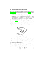
The INDEPENDENT SET problem remains NP-complete for cubic
planar graphs [GJS76]. A graph is called cubic if all vertices have
degree 3, i.e., all vertices are connected to exactly three vertices. A
graph is called planar if it can be drawn in the plane such that the
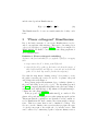
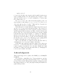
edges do not intersect. An example of a planar cubic graph is shown
in Figure 1.
14
13
8
2
0
15
9
1
7
3
4
6
5
10
11
12
Figure 1: Planar cubic graph
We consider a method that determines the maximal cardinality of
independent set of a planar cubic graph. Let us recall how the solution
to the maximum independent set can be encoded in the ground states
of a pair-interaction Hamiltonian HP .
Theorem 1 (Planar spin glass within a magnetic field)
Let G = (V, E) be a cubic planar. Determining the energy of the
ground states of the corresponding Hamiltonian
X
X
HP =
σz(k) σz(l) +
(7)
σz(k)
(k,l)∈E
k∈V
4
is equivalent to determining the maximum cardinality of independent
sets of G.
Proof. This has been shown in [Bar82] (see also [WB03]). We include
the proof here for completeness. We associate a variable Xk ∈ {0, 1}
to each vertex k ∈ V . There is an independent set whose cardinality
is at least v if and only if there is an assignment to the variables
{Xk | k ∈ V } such that
X
X
L=
Xk −
Xk Xl ≥ v .
(8)
k∈V
(k,l)∈E
This is seen as follows. If V ′ is an independent set whose cardinality
is at least v, then the assignment Xk = 1 for k ∈ V ′ and Xk = 0 for
k ∈ V \ V ′ fulfills inequality (8).
Now let X1 , . . . , Xn be an assignment that fulfills inequality (8).
If V ′ = {k | Xk = 1} is not
P an independent set, then we must have′
′
|V | ≥ v + p, where p := (k,l)∈E Xk Xl > 0 is the “penalty” for V
not being an independent set. Let (k̃, ˜l) ∈ E with X = X = 1. By
k̃
l̃
removing k̃ from V ′ (i.e. setting Xk̃ := 0) the cardinality of V ′ drops
by 1, while p drops by at least 1. After repeating this several times,
we end up with an independent set whose cardinality is at least v.
Setting Sk = 2Xk − 1 for all k ∈ V and observing that |E| = 32 |V |
for all cubic graphs, we obtain
L=−
1
1 X
1X
Sk Sl + |V | .
Sk −
4
4
8
k∈V
(9)
(k,l)∈E
For E = −4L+ 12 |V | we see that there exists an independent set whose
cardinality is at least k if and only if there is an assignment of values
to the variables Sk ∈ {−1, 1} (corresponding to the eigenvalues of σz )
such that
X
X
1
E=
Sk +
Sk Sl ≤ |V | − 4v .
(10)
2
k∈V
(k,l)∈E
Now it is clear that determining the minimal energy E is equivalent
to determining the maximal cardinality v of independent sets of G. ✷
In adiabatic quantum computing the initial Hamiltonian is chosen
as
HB =
X
k∈V
5
σx(k)
(11)
and the time-dependent Hamiltonian as
H(t) = (1 −
t
t
)HB + HP .
T
T
(12)
This Hamiltonian HP does not necessarily satisfy the locality conditions.
3
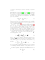
“Planar orthogonal” Hamiltonians
Due to the lattice structure of our resource Hamiltonian we need to
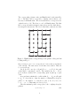
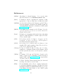
embed our graph into this structure. This can be done using planar
orthogonal embeddings of graphs [KW01]. This idea is inspired by
[KL02, RAS02]. We shall be concerned with embedding graphs into a
2D rectangular lattice.
Definition 1 (Planar orthogonal embedding)
A planar orthogonal embedding Γ of a graph G = (V, E) is a mapping
that
• maps vertices k ∈ V to lattice points Γ(k) and
• edges (k, l) ∈ E to paths in the lattice such that the images of
their endpoints Γ(k) and Γ(l) are connected and such that the
paths do not share any vertices (besides the endpoints).
Note that the map inserts “dummy vertices” if necessary to create
the paths connecting the vertices Γk and Γl . A planar orthogonal
embedding is shown in Figure 2.
Every planar graph with maximum degree 3 admits a planar orthogonal embedding on an ⌊n/2⌋ × ⌊n/2⌋. The algorithm presented
in [Kan96] computes efficiently such planar orthogonal embeddings of
graphs. We used AGD (Libary of Algorithms for Graph Drawing) to
compute the embedding [AGD02].
In the proposal of [KL02] the Hamiltonian HP is considered. The
planar orthogonal embedding gives a regular wiring among the qubits.
This means that the couplings are not spatially local. In contrast, we
need a Hamiltonian ĤP that contains only nearest-neighbor interactions. This is necessary that it can be simulated by HIsing . The
idea is to use the dummy vertices as wires that propagate the state
of a (real) vertex spin to the neighborhood of another vertex. This
can be achieved by constructing a path of adjacent dummy vertices,
6
15
11
12
10
5
1
14
0
2
13
8
4
6
3
7
9
Figure 2: Planar orthogonal embedding of the graph in Fig. 1
each interacting with its neighbor by a strong ferromagnetic coupling.
Furthermore, the first dummy at one end of this “dummy path” is
strongly ferromagnetically coupled to a vertex and the last dummy
at the other end is in the neighborhood of another real vertex, coupled to it via a usual antiferromagnetic interaction. The interaction
strength is chosen in such a way that it is always energetically better
when all dummies have the same state as the real vertex to which they
are connected to than to have a mismatch along the “ferromagnetic
path”.
Formally, this construction is as follows:
• The dummy vertices have no local σz term.
• The vertices Γ(k) have σz as local Hamiltonians.
• Let (k, l) ∈ E be an edge of G.
If Γk and Γl are adjacent, then the coupling between Γk and Γl
is chosen to be antiferromagnetic, i.e., σz ⊗ σz .
Otherwise there are m dummy vertices v1 , . . . , vm such that the
path (Γk , v1 , . . . , vm , Γl ) connects the vertices Γk and Γl . The
couplings between Γk and v1 and vi and vi+1 for i = 1, . . . , m − 1
are chosen to be ferromagnetic with coupling strength c, i.e.,
−c σz ⊗ σz . The coupling between vm and Γl is chosen to be
antiferromagnetic, i.e., σz ⊗ σz .
7
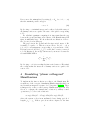
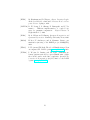
The corresponding “planar orthogonal Hamiltonian” is shown in Figure 3. The filled circles correspond to dummy vertices that do not
have any local Hamiltonian. The circles with indices correspond to the
original vertices of G. They have σz as local Hamiltonians. The thin
lines correspond antiferromagnetic interactions and the thick lines to
ferromagnetic interactions. The idea behind this construction is that
15
11
10
12
5
1
14
0
2
13
8
4
6
3
7
9
Figure 3: Hamiltonian corresponding to the planar orthogonal embedding in Fig. 2
there is a direct one-to-one correspondence between the ground states
of HP and ĤP . The same is true for the first excited states. This can
be seen as follows:
Let (k, l) ∈ E be an edge of G and (Γ1 , v1 , . . . , vm , Γl ) be the path
on the lattice connecting Γk and Γl . The variables SΓk , S1 , . . . , Sm ∈
{0, 1} indicate whether the corresponding qubit is spin up or spin
down.
A ground state satisfies the condition that S1 , . . . , Sm are all equal
to SΓk . To show this we define the number of mismatches along the
path to be the number of occurrences of SΓk 6= S1 , Si 6= Si+1 for
i = 1, . . . , m − 1. This number is denoted by δ.
Then the minimal possible energy (due to the couplings along the
path) is
c(−m + δ) − 1 .
(13)
8
If we remove the mismatches (by setting Si := SΓk for i = 1, . . . , m)
then the maximal possible energy is
−cm + 1 .
(14)
By choosing c = 3 minimal energy can be achieved only if the states of
all dummy vertices are equal to the state of the qubit corresponding
to Γk .
For adiabatic quantum computing it is important that the gap
between the ground and first excited states of the Hamiltonian at all
times is sufficiently large. We show that the modification of HP to
ĤP does not decrease this gap.
The gap between the ground and the first excited states of HP
is smaller or equal to 8. This is seen as follows. Let S1 , . . . , Sn ∈
{−1, +1} be an assignment corresponding to a ground state of HP .
Pick any vertex k and let l1 , l2 , l3 be at the three vertices connected
to k. By flipping Sk the energy can increase by at most 8 because the
relevant Hamiltonian is
σz(k)
+
3
X
σz(k) σz(li ) .
i=1
By choosing c = 9 it is seen that the first excited states of ĤP satisfy
the condition that the states all of dummy vertices are equal to the
vertex of Γk .
4 Simulating “planar orthogonal”
Hamiltonians
To implement the time-evolution according to the Hamiltonian ĤP
we make use of the concepts of simulating Hamiltonians that has been
used in nuclear magnetic resonance for a long time [EBW87]. These
techniques rely on the so-called average Hamiltonian approach. The
idea is to conjugate the natural time evolution by unitary control
operations uj , i.e., the total evolution is
uk exp(−iHtk )u†k . . . u†2 exp(−iHt2 )u†2 u1 exp(−iHt1 )u†1 ,
where the system evolves in an undisturbed way during periods of
length t1 , t2 , . . . , tk . If these periods are short compared to the time
9
scale of the natural evolution, the total dynamics is approximatively
the same as the evolution according to the average Hamiltonian
X tj
H :=
uj Hu†j
t
j
P
with t := j tj . Usually, the control operations on n particles are
assumed to be of the form
u := v1 ⊗ v2 ⊗ · · · ⊗ vn
where vj is a unitary acting on particle j. The design of simulation schemes for Hamiltonians with n particles interacting via pairinteractions leads to non-trivial combinatorial problems (e.g. [LCYY00,
DNBT01, WJB02, JWB02]). An experimental proposal for simulating
dynamics in optical systems is presented in [JVD+ 02].
Starting from the Ising Hamiltonian HIsing , we can implement the
Hamiltonian ĤP with time overhead (slow-down) 2c + 1 and 16 time
steps by interspersing the time evolution according to HIsing by local
operations in X ⊗ X ⊗ · · · ⊗ X, where X = {1, σx }.
Following the ideas of [LCYY00, WJB02] we construct a selective
decoupling scheme based on Hadamard matrices. Due to the special
form of HIsing it is sufficient to use the Hadamard matrix of size 4
only.
Our scheme consists of 4 subroutines that implement the following
couplings of ĤP :
1. horizontal σz ⊗ σz ,
2. vertical σz ⊗ σz ,
3. horizontal −c σz ⊗ σz , and
4. vertical −c σz ⊗ σz
The indices i, j enumerate the rows and the columns of the lattice.
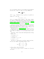
We denote the columns of the Hadamard matrix of size 4


1
1
1
1
 1 −1
1 −1 

W := 
 1
1 −1 −1 
1 −1 −1
1
by W (0, 0), W (0, 1), W (1, 0) and W (1, 1).
Let v = (v1 , v2 , v3 , v4 ) ∈ {−1, 1}4 be a column vector. We use the
abbreviation
10
“apply v at (i, j)”
to denote the following control sequence with 4 equally long time steps:
at the beginning and the end of the sth time step we apply σx on the
qubit at position (i, j) if vs = −1 and do nothing if vs = 1, where time
step s runs from 1 to 4.
Let v, v ′ ∈ {−1, 1}4 . One easily checks that applying v and v ′ at
adjacent lattice points changes σz ⊗ σz to hv, v ′ i σz ⊗ σz , where hv, v ′ i
denotes the inner product of v and v ′ . This is the key observation for
constructing the selective decoupling scheme.
In the first and second subroutines the length of the 4 time steps is
chosen to 1/4. Let us consider the first subroutine. The vertical couplings are automatically removed if we apply in rows with even indices
only W (0, 0) and W (1, 0) and in rows with odd indices W (1, 0) and
W (1, 1). The choice between W (a, 0) and W (a, 1) depends on which
horizontal interactions should remain or be switched off. Explicitly,
this choice is as follows. Choose W (a, 0) for the leftmost spin. If the
interaction between the spins (j − 1) and j should remain, then apply
the same W (a, b) to j as to (j −1). Otherwise (i.e. the coupling should
be switched off) apply the second possible W (a, b′ ) to j.
The second subroutine is obtained from the first subroutine by
exchanging the roles of rows and columns of the lattice.
In the third and fourth subroutines the length of the 4 time steps
is chosen to c/4. The third subroutine is obtained from the first subroutine by apply (−1)j v instead of v to the spin j. Finally, the fourth
subroutine is obtained from the third subroutine by exchanging the
roles rows and columns of the lattice.
Acknowledgments
This work was supported by grants of the BMBF project MARQUIS
01/BB01B.
We would like to thank Helge Rosé, Torsten Asselmeyer, and Andreas Schramm for interesting discussions that led us to consider this
problem. Therese Biedl, Thomas Decker and Khoder Elzein provided
interesting discussions on orthogonal graph drawing and installed the
graph drawing software.
11
References
[AGD02]
Algorithms for Graph Drawing. User manual, 2002.
www.ads.tuwien.ac.at /AGD/MANUAL/MANUAL.html.
[Bar82]
F. Barahona. On the computational complexity of Ising
spin models. J. Phys. A: Math. Gen., 15:3241–3253, 1982.
[DNBT01] J. L. Dodd, M. A. Nielsen, M. J. Bremner, and R. T. Thew.
Universal quantum computation and simulation using any
entangling Hamiltonian and local unitaries. LANL e-print
quant-ph/0106064, 2001.
[EBW87]
R. R. Ernst, G. Bodenhausn, and A. Wokaun. Principles
of nuclear magnetic resonance in one and two dimensions.
Clarendon Press, 1987.
[Fea01]
E. Farhi et al. A Quantum Adibatic Evolution Algorithm
Applied to Random Instances of an NP-complete Problem.
Science, 292:472, 2001.
[GJ79]
M. R. Garey and D. S. Johnson. Computers and Intractability: A guide to the Theory of NP-Completness.
W. H. Freeman and Company, 1979.
[GJS76]
M. R. Garey, D. S. Johnson, and L. Stockmeyer. Some
simplified NP-complete graph problems. Theoretical Computer Science, 1(2):237–267, 1976.
[JVD+ 02] E. Jane, G. Vidal, W. Dür, P. Zoller, and J. I. Cirac.
Simulation of quantum dynamics with quantum optical
systems. Quantum Information and Computation, 3(1):15,
2002.
[JWB02]
D. Janzing, P. Wocjan, and Th. Beth. Bounds on the
number of time steps for simulating arbitrary interaction
graphs. LANL e-print quant-ph/0203061, to appear in Int.
J. Found. Comp. Sci., 2002.
[Kan96]
G. Kant. Drawing Planar Graphs Using the Canonical
Ordering. Algorithmica, 16:4–32, 1996.
[KL02]
W. M. Kaminsky and S. Lloyd. Scalable Architecture
for Adiabatic Quantum Computing of NP-Hard Problems.
Quantum Computing & Quantum Bits in Mesoscopic Systems (Kluwer Academic 2003), see also LANL e-print
quant-ph/0211152, 2002.
12
[KW01]
M. Kaufmann and D. Wagner, editors. Drawing Graphs:
Method and Models, volume 2025 of Lecture Notes on Computer Science. Springer, 2001.
[LCYY00] D. W. Leung, I. L. Chuang, F. Yamaguchi, and Y. Yamamoto.
Efficient implementation of coupled logic
gates for quantum computation. Physical Review A,
61(4):042310–1–7, 2000.
[NC00]
M. A. Nielsen and I. Chuang. Quantum Computation and
Quantum Information. Cambridge University Press, 2000.
[RAS02]
H. Rosé, T. Asselmeyer, and A. Schramm. Private communication (meeting of the BMBF project MARQUIS).
2002.
[WB03]
P. Wocjan and Th. Beth. The 2-local Hamiltonian problem
encompasses NP. LANL e-print quant-ph/0301087, 2003.
[WJB02]
P. Wocjan, D. Janzing, and Th. Beth. Simulating arbitrary pair-interactions by a given Hamiltonian: graphtheoretical bounds on the time complexity. Quantum Information & Computation, 2(2):117, 2002. see also LANL
e-print quant–ph/1010677.
13