Download Power Viewer Plus - Software Manual

R&S Power Viewer Plus
Software Manual
R&S® Power Viewer Plus
V 5.6
Printed in Germany
Manual
1
R&S Power Viewer Plus
Dear Customer,
R&S® is a registered trademark of Rohde & Schwarz GmbH & Co. KG.
R&S® is referred to as R&S throughout this manual.
Mac and Mac OS are trademarks of Apple Inc.,
registered in the U.S. and other countries.
Microsoft and Windows are trademarks of Microsoft Corporation
in the United States and/or other countries.
Trade names are trademarks of their respective owners.
© 2011 Rohde & Schwarz GmbH & Co. KG
81671 Munich, Germany
Printed in Germany – Subject to change – Data without tolerance limits is not binding.
Manual
2
R&S Power Viewer Plus
1
Contents
1
Contents
3
2
Overview
7
3
Key Software Features
8
4
Power Sensor Technologies
13
4.1
Thermal Power Sensors .........................
13
4.2
CW Power Sensors ............................. 13
4.3
Multi-Path Diode Power Sensors ................... 14
4.4
Average Power Sensors .........................
14
4.5
Wideband Diode Power Sensors ...................
14
5
6
7
8
9
Manual
Contents
Uncertainty Calculation
16
5.1
Measurements at –10 dBm .......................
17
5.2
Measurements at –50 dBm .......................
18
5.3
The Influence of Mismatch ........................ 19
Software Installation
21
6.1
System Requirements ........................... 21
6.2
Installation on Windows-Based Systems .............. 22
6.3
Installation on Linux-Based Systems ................ 23
6.4
Installation on Mac OS X .........................
6.5
Sensor Firmware Requirements .................... 28
6.6
Supported R&S NRPZ Sensors .................... 29
6.7
Running Multiple Instances .......................
Command Line Options
25
30
31
7.1
General Options ............................... 31
7.2
Setting the Application Style ....................... 33
Connecting Sensors to the PC
34
8.1
Using Multiple Sensors .......................... 34
8.2
Using USB Extension Hardware ....................
8.2.1 R&S NRP-Z3 Active USB Adapter ............
8.2.2 R&S NRP-Z4 Passive USB Adapter ..........
8.2.3 R&S NRP-Z5 Sensor Hub ..................
8.2.4 Third-Party Products ......................
Configuring the Application
35
35
35
36
37
38
9.1
Drawing Performance ........................... 38
9.2
Hardcopy Settings .............................. 40
9.3
Timeout-Related Settings ........................ 41
9.4
USB-Related Settings ........................... 42
9.5
USB Device Tree ..............................
9.6
Debug Options ................................ 44
43
3
R&S Power Viewer Plus
Contents
10
Setting the Application Colors
45
11
First Steps
47
11.1 Numeric Entry Fields ............................ 48
11.2 The Menu Bar .................................
11.2.1 File ..................................
11.2.2 Sensor ................................
11.2.3 Measurement ...........................
11.2.4 Data Processing .........................
11.2.5 Window ...............................
11.2.6 Help ..................................
11.3 The Toolbar ..................................
49
49
49
51
52
53
54
55
11.4 Selecting a Sensor ............................. 55
12
11.5 General Measurement Settings ....................
56
Hardcopy Features
58
12.1 Print Report .................................. 58
12.2 Copy to Clipboard ..............................
59
12.3 Save Graphics to File ...........................
59
13
The Message Log
60
14
Channel Assignment
61
15
Continuous Power Measurement
62
15.1 Settings ..................................... 62
15.2 Numerical Data View ............................ 64
15.3 Negative Power Readings ........................ 65
15.4 Accuracy of Peak Power Measurements .............. 65
15.5 Relative Measurements .......................... 66
15.6 Analog Meter ................................. 67
15.7 Trend Chart .................................. 68
15.8 Histogram Display .............................. 69
15.9 Q-Q-Plot ..................................... 70
16
Trace Measurements
71
16.1 Measurement Settings .......................... 71
16.2 Custom Settings ...............................
76
16.3 Graphical Trace View ...........................
77
16.4 Context Menu ................................. 78
16.5 Trace Representations ..........................
79
16.6 View Modes .................................. 80
16.7 Lines .......................................
82
16.8 Reference Trace ............................... 82
16.9 Using Markers ................................
16.9.1 Pulse Width Measurements .................
16.9.2 Pulse Rise-Time Measurements .............
16.10 Zooming .....................................
16.10.1 Time Zoom ............................
16.10.2 Level Zoom ............................
Manual
83
84
85
86
86
87
4
R&S Power Viewer Plus
Contents
16.11 Automatic Pulse Measurement .................... 88
16.11.1 Measurement Results ..................... 91
16.12 Common Measurement Tasks ..................... 93
17
Statistics
94
17.1 Settings ..................................... 94
17.2 Graphical Data View ............................ 96
17.3 PDF Mode ................................... 97
17.3.1 PDF Background Information ............... 98
17.4 CDF Mode .................................. 100
18
17.5 CCDF Mode .................................
101
Timeslot Mode
102
18.1 Settings .................................... 102
18.2 Graphical Data View ........................... 105
19
Multi-Channel Power Measurements
106
19.1 Channel Configuration .......................... 107
19.2 Measurement Settings .......................... 108
19.3 Mathematical Expressions ....................... 109
20
Script-Based Measurement
110
20.1 Script Syntax ................................
20.1.1 Variables .............................
20.1.2 Predefined Variables .....................
20.1.3 Variable Value Assignments ...............
20.1.4 Equations .............................
20.1.5 Comments ............................
20.1.6 Suppressing Output .....................
20.1.7 Waiting Periods ........................
20.1.8 Loops ................................
20.1.9 Defining Devices ........................
20.1.10 Waiting for Measurement Completion .........
20.1.11 SCPI Commands and Queries ..............
20.1.12 Reading Scalar Results ...................
20.1.13 Reading Array Results ...................
20.1.14 Converting Readings .....................
20.1.15 Printing to the Log Window ................
20.1.16 Displaying Scalar Results .................
20.1.17 Displaying Array Data Numerically ...........
20.1.18 Displaying Array Data as a Bargraph .........
20.1.19 Displaying Array Data as a Trace ............
20.1.20 Saving Array Data to Text File ..............
20.1.21 Sending Data to Processing Panels ..........
20.2 Triggered Average Power Measurement .............
111
111
111
112
113
113
113
113
114
114
115
115
116
116
117
117
117
117
118
118
119
119
120
20.3 Burst Power Measurement ......................
121
20.4 Buffered-Mode Measurements .................... 122
21
Manual
Data Processing Panels
123
21.1 The Data Log ................................
21.1.1 Settings ..............................
21.1.2 The Context Menu ......................
21.1.3 The Time Line Indicator ...................
21.1.4 Zooming ..............................
21.2 Limit Monitoring ..............................
125
126
129
130
130
131
5
R&S Power Viewer Plus
22
Contents
21.2.1 Settings ..............................
21.2.2 Configuring the Server ...................
21.2.3 Client Connections ......................
21.3 Statistical Analysis ............................
21.3.1 Histogram Display .......................
21.3.2 Q-Q-Plot .............................
21.3.3 The Context Menu ......................
21.3.4 Analysis-Panel Settings ...................
132
134
136
137
138
139
140
141
Updating the Sensor Firmware
142
22.1 Recovering from a Failed Update .................. 144
23
Programming Guide
145
23.1 Sensor Resource Strings ........................ 145
23.2 Numeric Results ..............................
146
23.3 Opening and Closing the Sensor Connection ......... 146
23.4 Multiple Sensors ..............................
146
23.5 Error Handling ...............................
147
23.6 Zeroing ..................................... 147
23.7 Identifying a Sensor (*IDN?) ...................... 148
23.8 Continuous Average Power Measurement ........... 148
23.9 Trace Measurements ..........................
23.9.1 Single-Shot Events ......................
23.9.2 Peak Trace Data ........................
23.9.3 Automatic Pulse Measurement .............
151
153
154
155
24
Customer Support
157
25
Open Source Acknowledgment
157
26
Licenses
158
26.1 GNU Lesser General Public License (LGPL) 2.1 ....... 158
Manual
6
R&S Power Viewer Plus
2
Overview
Overview
The new R&S NRP-Z power sensors from Rohde & Schwarz represent
the latest in power measurement technology. They offer all the
functionality of conventional power meters, and more, within the small
housing of a power sensor. The USB interface on an R&S NRPZ sensor
enables operation with an R&S NRP power meter, or with a PC running
under either Microsoft® Windows®, Mac OS X, or Linux.
R&S Power Viewer Plus is an easy-to-use, feature-packed software
package that offers capabilities beyond those of a regular power meter.
It simplifies measurement tasks, such as average-power, timeslot,
statistics and trace measurements. In addition, up to four sensors can
be utilized for measuring average power simultaneously. Results, such
as the reflection coefficient or gain, can be computed from the
measured values.
Particularly the capabilities for use with a desktop or laptop PC make an
R&SNRPZ sensor an ideal and cost-effective solution for lab testing or
for automated systems. The rugged design is suitable for use in the
field for performing such tasks as servicing antenna systems.
This manual describes the installation and use of the
Power Viewer Plus software. This application is part of the
R&S®NRP Toolkit and is available free of charge from the
Rohde & Schwarz website.
To enable integration of the sensor into custom ATE systems, a
versatile and powerful VXI PnP driver is available for
Microsoft® Windows®, Mac OS X, and Linux-based systems. Coding
examples can be found at the end of this manual.
Manual
7
R&S Power Viewer Plus
3
Key Software Features
Key Software Features
Power Viewer Plus is powerful PC software that simplifies many
measurement tasks. This software is part of the R&S NRP Toolkit and
is available free of charge. The following overview lists some of the key
features that Power Viewer Plus offers.
•
Measuring the average and peak powers and viewing the
numeric results. Optionally, adding an analog bar display, a
trend chart or statistical analysis.
Fig. 3.1: Viewing measurement results.
•
Viewing the RF power envelope down to a resolution of
5 ns/div; measuring pulse parameters with automatic pulse
analysis; using markers, and measuring within time gates.
Fig. 3.2: Pulse measurement.
Manual
8
R&S Power Viewer Plus
Key Software Features
•
Measuring the average power of up to 16 sensors, and
optionally computing results from the measured values.
Fig. 3.3: Measuring average power.
•
Viewing the average and peak powers for up to 16 consecutive
timeslots in a bar chart.
Fig. 3.4: Viewing average and peak powers.
Manual
9
R&S Power Viewer Plus
Key Software Features
•
Performing statistical CCDF, CDF, or PDF analysis of the
envelope power.
Fig. 3.5: Statistical analysis.
•
Recording up to 4 channels of any measured data to memory
and/or to a file.
Fig. 3.6: Recording measured data.
Manual
10
R&S Power Viewer Plus
Key Software Features
•
Performing 4-channel statistical analysis on any measured
data.
Fig. 3.7: Four-channel statistical analysis.
•
Configuring 16-channel limit monitoring for any measured data;
optionally, sending limit violations to a remote host via a TCP/IP
server.
Fig. 3.8: Limit monitoring.
Manual
11
R&S Power Viewer Plus
Key Software Features
•
Creating custom measurements in script mode.
Fig. 3.9: Script mode for custom measurements.
Please note that some of the features listed above are only supported
by certain R&S NRP-Z power sensors. For example, thermal sensors
do not provide statistical signal analysis or trace measurements.
Manual
12
R&S Power Viewer Plus
4
Power Sensor Technologies
Power Sensor Technologies
Rohde & Schwarz offers a large choice of USB power sensors that use
different technologies and cover a wide range of frequencies and power
levels. This chapter briefly outlines the differences between the sensor
technologies and indicates which sensor would best fit certain
measurement tasks.
All R&S NRPZ power sensors are standalone instruments that contain
the detector, the analog circuitry, and the digital signal processing in a
single housing. The entire instrument is fully characterized during the
production process, which eliminates the need for later calibration using
a reference power source.
Zeroing is generally only required for measuring low power levels, in
which case the zeroing offset, noise, and drift stated in the specification
sheet contribute to the overall accuracy.
4.1
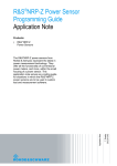
Thermal Power Sensors
Thermal sensors use a load resistor for converting the RF power into
heat. The temperature difference between this resistor and the
surrounding area is measured by thermocouples. The resulting DC
voltage is proportional to the RF power.
coaxial RF feeder
co-planar line
thermal
transducer
1 mm
tapered
transmisssion
Fig. 4.1.1: Detector design in thermal power sensor.
The Rohde & Schwarz thermal power sensors can be used from DC up
to their specified upper frequency limit. The dynamic range is typically in
the order of 55 dB and starts at power levels of around –35 dBm.
Thermal power sensors provide the highest accuracy and linearity of all
power sensors on the market. Their measurements are not influenced
by the modulation or harmonics, and the results always represent the
average signal power.
However, the nature of the underlying sensor technology limits the
dynamic range. Furthermore, the measurement speed is generally
slower than that of diode sensors. Thermal sensors cannot measure the
envelope of an RF signal.
4.2
CW Power Sensors
CW sensors are simple diode sensors that contain a half-wave or
full-wave rectifier as the detector element. At power levels below
-20 dBm, the diode characteristic provides an almost linear relationship
between the detector output voltage and the RF power. This power
range is referred to as the square-law region of the detector diode.
CW sensors typically use the diode at power levels beyond the
square-law region, and the software must compensate for the resulting
Manual
13
R&S Power Viewer Plus
Power Sensor Technologies
non-linearities. With CW signals, this compensation is possible, and
the sensor provides correct readings of the average RF power.
Modulated or pulsed signals, as well as signals containing harmonics,
may lead to large measurement errors at levels that exceed the
detector's square-law region.
Due to these limitations, the Rohde & Schwarz NRPZ product range
does not include CW sensors.
4.3
Multi-Path Diode Power Sensors
The Rohde & Schwarz multi-path diode sensors use up to three
independent full-wave diode detectors. These detectors, along with their
analog and digital signal processing, are referred to as paths. Each path
is designed for operation in a separate power range, with a 6 dB overlap
between the paths.
Fig. 4.3.1: Multi-path diode sensor design.
The data from all paths is processed in parallel. For each power level
within the specified sensor limits, at least one path operates within the
detector's square-law region and delivers an output signal that is
proportional to the RF energy. The sensor software automatically
determines the path that best fits the incident RF power.
As a result, these sensors exhibit little sensitivity to modulation and
harmonics. The sensors always measure the average signal power at a
performance level that is close to that of thermal sensors. Due to the
ease of use and excellent performance offered by these sensors,
Rohde & Schwarz calls these devices R&S Universal Power Sensors.
The universal power sensors' dynamic range and measurement speed
are higher than can be achieved with thermal sensors. For most signals
and measurement tasks, universal power sensors are ideal devices.
These sensors also allow measurement of the RF envelope, but the
sampling rate of about 150 kHz must be considered as a limiting factor
in such cases.
4.4
Average Power Sensors
The Rohde & Schwarz Average Power Sensors also use three diode
paths. Unlike the universal power sensors, the detector design used for
average power sensors allows an RF frequency as low as 9 kHz. Due to
this detector design, the bandwidth is lower. Consequently, this sensor
is only intended for performing average power measurements.
4.5
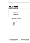
Wideband Diode Power Sensors
Wideband diode sensors use a single full-wave diode detector and
operate it across the entire useful power range. The detector's
bandwidth is much higher than with CW sensors, and the sample rate is
in the order of 80 MHz.
Manual
14
R&S Power Viewer Plus
Power Sensor Technologies
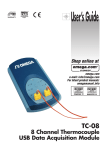
Fig. 4.5.1: Wideband power sensor design.
Similar to CW sensors, the wideband diode sensor's digital signal
processing circuitry compensates the non-linear diode characteristic in
realtime. Due to the wider bandwidth and fast sampling rate, this is even
possible for fast amplitude changes (AM) of the RF envelope.
Wideband diode sensors are ideal when the RF envelope should be
measured, e.g. for the analysis of pulsed signals. Additionally, these
devices can measure the signal statistics, such as the PDF, CDF,
CCDF, and average power for modulated signals.
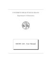
The following chart shows the relationship between power levels and
applications that generally fit a wideband diode sensor.
Average Power,
Av. Power,
fmod < BW
fmod > BW
Peak Power
Envelope (Averaged)
Envelope (Real Time)
-60 dBm
-20 dBm
+23 dBm
Fig. 4.5.2: Wideband power sensor applications.
At power levels below –20 dBm (square-law region), these sensors
exhibit little sensitivity to modulation and harmonics. Average power
measurements are possible down to a level of about –60 dBm.
For higher power levels, care must be taken when the RF envelope is
amplitude modulated at frequencies that exceed the detector's analog
bandwidth. In such cases, it is no longer possible to compensate the RF
envelope in realtime, and measurement errors in the order of several
percent may occur.
The wider bandwidth used by these sensors generally implies a higher
noise floor. Average power measurements overcome this issue by
using averaging techniques. When taking single-shot measurements,
however, the higher noise floor must be considered.
This is especially the case with peak power measurements. Please see
the chapter 15.4, "Continuous Power Measurements – Accuracy of
Peak Power Measurements" in this document for more details.
It must also be noted that triggering is always a realtime process that is
based on samples that have not yet been subject to averaging. As a
result, power levels in the order of –20 dBm or higher are required when
Manual
15
R&S Power Viewer Plus
Power Sensor Technologies
using the sensor's internal trigger feature. Decreasing the sensor's
bandwidth decreases the noise floor and, therefore, also decreases the
lower trigger-level limit.
5
Uncertainty Calculation
This chapter briefly explains how to calculate the measurement
uncertainty based on the figures provided in the sensor's specifications.
The data sheet lists the absolute uncertainty for power measurements
in dB depending on the power level and frequency. Other contributors,
such as zero offset or noise, are provided in watts and can be
converted into dB using the following equation.
e=10 dB⋅log
P P

P
This equation uses P as the power level of interest and ΔP as the
relative error. The result is the error e in dB.
Uncertainties are statistical measures, and they must be added by
summing up the squared uncertainties and then calculating the square
root:
U = U 21U 22U 23 
This equation can be used for uncertainties in logarithmic scale (dB) or
in percent (%).
Uncertainties are commonly provided in dB, but the following equation
permits conversion into percent:
U dB
U %=100%⋅10
10 dB
−1
To gain a simple approximation, the following formula can be used:
U %≈10⋅ln 10⋅U dB=23⋅U dB
Manual
16
R&S Power Viewer Plus
5.1
Uncertainty Calculation
Measurements at –10 dBm
The power level range from –10 dBm to 0 dBm is widely used.
Therefore, our first example here calculates the absolute uncertainty for
the R&S NRP-Z11 when measuring a CW signal at 2 GHz and at a
power level of –10 dBm. The temperature shall be 30 ºC.
All values marked with an arrow (►) are taken from the R&S NRPZxx
Power Sensor Specifications that are available on the Rohde & Schwarz
website.
Power level in W
► Used path
100 µW
2
► Uncertainty for absolute
power measurements
0.077
► Zero Offset
► Zero Drift
47 nW
10 nW
► Measurement noise
Multiplier for 40 ms integration
Time is sqrt(10.24s/T)
6.3 nW
Total expanded uncertainty
x 16
= 100.8 nW
dB
0.002 dB
0.0004 dB
0.004
dB
0.077
1.79
dB
%
The example shows that the influence of zero offset and drift is
negligible. Consequently, zeroing of the sensor is not required when
performing practical measurement tasks. The integration time can be
set to a very short value of 40 ms. This means that an averaging count
of one, combined with two chopper cycles and a measurement window
(aperture) of 20 ms, is sufficient.
The total integration time is twice the aperture time multiplied by the
averaging filter count.
Manual
17
R&S Power Viewer Plus
5.2
Uncertainty Calculation
Measurements at –50 dBm
This example calculates the absolute uncertainty for the R&S NRPZ11
when used for measuring a CW signal at 2 GHz and at a very low
power level of –50 dBm. The temperature shall be 30 ºC.
All values marked with an arrow (►) are taken from the R&S NRPZxx
Power Sensor Specifications that are available from the
Rohde & Schwarz website.
Power level in W
► Used path
10 nW
1
► Uncertainty for absolute
power measurements
0.081
► Zero offset after zeroing
► Zero drift after zeroing
104 pW
35 pW
► Measurement noise
Multiplier for 1.28 s integration
time is sqrt(10.24s/T)
65 pW
Total expanded uncertainty
x 2.8
= 182 pW
dB
0.045 dB
0.0015 dB
0.078
dB
0.12
2.8
dB
%
After zeroing, the absolute accuracy is 0.12 dB when using an
integration time of 1.28 s. This integration time can be achieved with an
average filter count of 32 and a measurement window of 20 ms. Further
improvement of the uncertainty is possible by increasing the averaging
filter count.
The total integration time is twice the aperture time multiplied by the
averaging filter count.
Manual
18
R&S Power Viewer Plus
5.3
Uncertainty Calculation
The Influence of Mismatch
Power sensors are always calibrated to measure the power of the
incident RF wave. This means that the sensor corrects the reading for
the internal losses and reflections. As a result, different power sensors
that were connected to an ideal 50 ohm source would all show exactly
the same result.
In the real world, however, neither the power sensor nor the source
match an impedance of 50 ohms exactly. The reflection that is caused
by the power sensor itself is specified by the standing wave ratio
(SWR), which is typically around 1.2. This means that a small portion of
the RF wave is reflected back towards the source as a return wave. An
ideal source would absorb this return wave entirely. Since the power
sensor is calibrated to measure the incident wave and compensates for
its own reflections, the reading is correct.
Real signal sources are not ideal either. They also reflect a portion of
the return wave back to the power sensor. This portion adds to the
incident RF wave and influences the measurement result.
The uncertainty calculations in the previous chapter did not include the
error caused by mismatch. The following equation shows the minimum
and maximum possible incident power based on the reflection
coefficient of the source and the load:
P GZ0
1r G r L 
P i 
2
PGZ0
1−r G r L 
2
PGZ0: Power from signal source
Pi: Incident power to power
sensor
rG: Generator reflection
coefficient
rL:
Load reflection coefficient
Depending on the phase angle, the incident power varies between the
left and right term of the equation. The following equations can
approximate the maximum relative deviation εmax between the source
power PGZ0 and the incident power Pi:
 max %≈200 % r G r L
 max dB≈8.7 dB r G r L
for  max 20 %
for max 1 dB
Uncertainty calculations use statistical figures instead of the εmax errors
from the equations above. The following equation shows the
relationship between the expanded uncertainty (k = 2) and the error.

U dB=2⋅ max dB
2
This shows that the expanded uncertainty used for the uncertainty
calculation is higher than the maximum error.
Manual
19
R&S Power Viewer Plus
Uncertainty Calculation
Data sheets often express the impedance matching of a device as a
standing wave ratio (SWR). The relationship between the SWR and the
reflection coefficient is expressed by the following equations:
s=
1r L
1−r L
r L=
s−1
s1
The example below demonstrates the influence of mismatch caused by
a signal source that is directly connected to a power sensor:
Load:
Source:
R&S NRPZ11
R&S SMBV100A
SWR = 1.2
SWR = 1.6
rL = 0.09
rG = 0.23
UdB = 2 · 0.707 · ± 8.7 dB · 0.09 · 0.23 = ± 0.25 dB
Manual
20
R&S Power Viewer Plus
6
Software Installation
Software Installation
The following section outlines the process for installing
Power Viewer Plus on various platforms.
6.1
System Requirements
If the sensors are to be controlled by a PC rather than by using the
R&S NRP base unit, certain prerequisites must be fulfilled.
Hardware requirements
• Desktop PC or laptop, or an Intel-based Apple Mac
• Keyboard and mouse
• 800 x 600 screen resolution (1024 x 768 recommended)
• USB 1.1 or 2.0 interface
• Multi-TT based USB hub architecture recommended
• R&S NRP-Z3, R&S NRP-Z4, or R&S NRP-Z5 adapter
Operating systems (choice of)
• Microsoft® Windows® XP 32-Bit
• Microsoft® Windows® 7 32/64-Bit
• Mac OS X
• 32-Bit Linux distribution with kernel ≥ 2.6.x
(e.g. Ubuntu 10.4 LTS x86, 11.4 x86)
R&S software packages
• R&S NRP Toolkit. It provides the required USB drivers.
• The Power Viewer Plus software is supplied with the R&S NRP
Toolkit.
Manual
21
R&S Power Viewer Plus
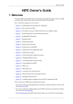
6.2
Software Installation
Installation on Windows-Based Systems
The application is part of the R&S NRP Toolkit. This toolkit contains all
required USB drivers, as well as toolkit applications and
Power Viewer Plus.
1. Disconnect all NRP-Zxx power sensors from the PC.
2. Start the R&S NRP Toolkit installer and follow the instructions.
3. In the Choose Components window, you must enable the USB
drivers if the toolkit has never been installed before. If a
previous R&S NRP Toolkit installation is found, the installer
may offer an option to update the drivers. It is highly
recommended that you enable the USB driver update.
4. Enable R&S NRP Toolkit if you need additional toolkit
programs, such as the S-parameter update, or the classic
Power Viewer.
5. Enable R&S Power Viewer Plus.
Fig. 6.2.1: R&S NRP Toolkit installer.
After the installation has completed, the sensors can be connected to
the PC. If the USB drivers were updated or newly installed, recognizing
the sensor may take more time when it is plugged in for the very first
time.
Manual
22
R&S Power Viewer Plus
6.3
Software Installation
Installation on Linux-Based Systems
This application is part of the R&S NRP Toolkit. In contrast to the
Windows R&S NRP Toolkit, the Linux version contains the following
components:
•
•
•
•
•
•
NrpZ
Kernel module
NrpLib
Low-level driver
RsNrpZ
VXI PnP driver
HTML help files for the VXI PnP driver
Power Viewer Plus and PDF manual
Example programs for use with VXI PnP driver
The toolkit comes as a self-extracting archive that must be run with root
user permissions:
# sudo ./NrpLinuxPckg_<date>.run
Running the installer requires the following tools and packages to be
present in the system:
•
•
•
•
dialog, base64, tar, gcc
ia32-libs (on amd64 systems only)
Kernel modules under /lib/modules/<version>
Kernel headers under /usr/include/linux
The self-extracting archive first extracts it's content to a temporary
directory under /tmp and then transfers control to the installation script
in this directory.
Fig. 6.3.1: R&S NRP Toolkit installer for Linux.
If the basic system requirements are met, the screen shown above
should appear and prompt the user to confirm if the installation should
start.
Next, the legal terms are displayed. Use q to quit this screen, and then
accept the license terms.
Manual
23
R&S Power Viewer Plus
Software Installation
Fig. 6.3.2: Accepting the license terms.
The license terms must be accepted in order to continue with the
installation.
The following screen allows the user to select the items for installation.
The first entry compiles the kernel module and installs all required
drivers. This step is crucial for operating the sensors on a Linux system.
It is also required for running the Power Viewer Plus application or for
compiling the example programs.
Fig. 6.3.3: Installation items.
After the installation has been completed, the Power Viewer Plus
application is launched by a start script:
PowerViewerPlus
This script first verifies that it is not being called with super-user
privileges. Then it starts the Power Viewer Plus binary.
Manual
24
R&S Power Viewer Plus
6.4
Software Installation
Installation on Mac OS X
This application is part of the R&S NRP Toolkit. In contrast to the
Windows R&S NRP Toolkit, the Mac OS X version contains the
following components:
•
•
•
•
•
RsNrpLib.framework
Low-level driver
RsNrpz.framework
VXI PnP driver
HTML help files for the VXI PnP driver
Power Viewer Plus and PDF manual
Example programs for use with the VXI PnP driver
The toolkit comes as a .dmg disk image that can be mounted by
double-clicking the file in the Mac OS X Finder. This image contains the
NrpToolkit.mpkg installer. Double-click this entry in the disk image view.
Fig. 6.4.1: Contents of the .dmg image.
Manual
25
R&S Power Viewer Plus
Software Installation
The welcome message provides an overview of the packages that are
part of the installer and indicates their default installation location.
Fig. 6.4.2: R&S NRP Toolkit installer for Mac OS X.
After the legal notices have been accepted, the installer presents a
menu that allows selection of the components for installation.
The first entry contains the driver frameworks and is mandatory.
Fig. 6.4.3: Installation selection.
The Application Development entry is optional and is not enabled by
default. It installs simple C programs that use the VXI PnP driver. These
small programs may be used as starting points for your own
implementations.
Manual
26
R&S Power Viewer Plus
Software Installation
After successful installation, the Power Viewer Plus application can be
started from the Rohde-Schwarz folder that was created in the
Mac OS X application directory.
Fig. 6.4.4: The "Rohde-Schwarz" folder.
Manual
27
R&S Power Viewer Plus
6.5
Software Installation
Sensor Firmware Requirements
Power Viewer Plus may require newer firmware versions on certain
power sensors. Please see the firmware update section in this manual
for more details on updating the sensor firmware. The latest firmware
files are available free of charge from the Rohde & Schwarz website.
R&S NRP-Z8x
R&S NRP-Z1x
R&S NRP-Z2x
R&S NRP-Z3x
R&S NRP-Z5x
Manual
1.16 or later (1.20 recommended)
4.08 or later
4.08 or later
4.08 or later
4.08 or later
28
R&S Power Viewer Plus
6.6
Software Installation
Supported R&S NRPZ Sensors
The following table provides an overview of the sensors that are
supported in Power Viewer Plus.
Sensor
USB
ID
NRP-Z11
0x0C
Cont
●
Supported Measurement
Trace
Timeslot
Statistics
●
●
NRP-Z21
0x03
●
●
●
NRP-Z211
0xA6
●
●
●
NRP-Z22
0x13
●
●
●
NRP-Z221
0xA7
●
●
●
NRP-Z23
0x14
●
●
●
NRP-Z24
0x15
●
●
●
NRP-Z31
0x2C
●
●
●
NRP-Z41
0x96
●
●
●
NRP-Z51
0x16
●
NRP-Z52
0x17
●
NRP-Z55
0x18
●
NRP-Z56
0x19
●
NRP-Z57
0x70
●
NRP-Z58
0xA8
●
NRP-Z91
0x21
●
NRP-Z81
0x23
●
●
●
●
NRP-Z85
0x83
●
●
●
●
NRP-Z86
0x95
●
●
●
●
NRP-Z27
0x2F
●
NRP-Z28
0x51
●
●
●
NRP-Z37
0x2D
●
NRP-Z92
0x62
●
NRP-Z98
0x52
●
NRPC33
0xB6
●
NRPC40
0x8F
●
NRPC50
0x90
●
NRPC33-B1
0xC2
●
NRPC40-B1
0xC3
●
NRPC50-B1
0xC4
●
FSH-Z1
0x0B
●
FSH-Z18
0x1A
●
If no sensor is detected, Power Viewer Plus automatically activates a
simulated sensor called NRP-Z00.
The vendor ID for all R&S NRP-Zxx sensors is 0x0AAD.
Manual
29
R&S Power Viewer Plus
6.7
Software Installation
Running Multiple Instances
Only one instance of Power Viewer Plus can be run at a time. This
limitation is required, because the low-level drivers do not support
simultaneous access to the sensors from multiple applications.
Power Viewer Plus checks to see if any other instance is already
running on the system. If so, a warning message appears.
Fig. 6.7.1: Warning message indicating that an application is already
running.
Power Viewer Plus does not detect if any other application is already
accessing the low-level drivers. For this reason, it is advisable to close
all other R&S NRP-Z-related applications before starting
Power Viewer Plus.
Manual
30
R&S Power Viewer Plus
Command Line Options
7
Command Line Options
7.1
General Options
The Power Viewer Plus software supports a set of command line
options that affect the application's look and feel as well its startup
behavior:
--native
The user interface look is left as native as possible.
--classic-pv
This option starts Power Viewer Plus in a mode in which it only displays
the continuous power measurement window. This is similar to the
classic Power Viewer application:
• Disables all features but the continuous power measurement.
• Always starts with a fixed application window size.
• Continuous power measurement is activated.
• The analog bar and trend display are not available.
• The measurement starts automatically if a sensor is detected.
--no-splash
This option omits the initial splash screen and speeds up the application
startup.
--project <file>
This option loads a specific project file at startup. If the application is
available, the default project file is written. If the specified project file is
not available, the default settings are applied.
--sensor <sensor>
This option includes –no-splash and omits the initial sensor scanning.
Instead, the specified sensor is made available regardless of its
physical availability. The sensor must be defined by the sensor type and
by its serial number (for example: “Z11,123456”).
--no-multi
Disables the multi-channel measurement mode.
Manual
31
R&S Power Viewer Plus
Command Line Options
--no-flash
Disables the firmware flash dialog.
--no-timeslot
Disables the timeslot measurement mode.
--no-statistics
Disables the statistics measurement mode.
--no-trace
Disables the trace measurement mode.
--no-scripting
Disables the scripting measurement mode.
--no-datalog
Disables the data log window.
--no-analysis
Disables the data analysis window.
--no-monitor
Disables the limit monitoring window.
--debug
Writes additional log messages to the message log window. This may
be useful for debugging software problems.
Manual
32
R&S Power Viewer Plus
7.2
Command Line Options
Setting the Application Style
The style of the Power Viewer Plus user interface can be changed using
the -style command-line option. Changing the style might be useful if
the application should use the operating system's look and feel. By
default, Power Viewer Plus uses an internal style that is independent of
the underlying operating system.
-style <style>
<style>
User Interface Example
Plastique
Cleanlooks
Windows
Motif
WindowsXP
Manual
33
R&S Power Viewer Plus
8
Connecting Sensors to the PC
Connecting Sensors to the PC
Please see your R&S NRP-Z power sensor's manual for information on
how to put the sensor into operation. Follow these instructions to
prevent damage to the sensor, particularly if you are putting it into
operation for the first time.
The following section provides additional information that is related to
the USB interface or to operating multiple sensors simultaneously.
8.1
Using Multiple Sensors
If multiple sensors need to be connected to a single computer, check to
ensure that the overall current requirements for operating all sensors
can be met. Each single sensor draws between 300 mA and 500 mA,
depending on the sensor type.
Example:
The R&S NRP-Z81 sensor is rated at up to 500 mA supply current.
Using four sensors simultaneously on one hub requires a total current
of at least two amperes. Many consumer hubs cannot provide this
current over a long period of time, even if they are rated for this value.
For industrial-grade applications, it is advisable to use USB hubs for a
DIN rail mount that can provide up to one ampere per USB port and run
off a 24 V power supply. These two manufacturers provide such
devices:
• Beckhoff ( www.beckhoff.com ) CU8005
• Lütze ( www.luetze.de ) 745581 DIOHUB USB 4
Other industrial or office-type hubs that have shown good performance
at the time of writing (2009) are:
• BELKIN® Hi-Speed USB 2.0 7-Port Hub F5U237eaAPL-S
• Digi® Hubport/4c or Hubport/7c
The following hub specifications are crucial when multiple power
sensors shall be connected to the hub:
• Multi-TT switched architecture
• Individual port power management, 500 mA per channel
Manual
34
R&S Power Viewer Plus
Connecting Sensors to the PC
8.2
Using USB Extension Hardware
8.2.1
R&S NRP-Z3 Active USB Adapter
The figure shows the configuration with the R&S NRP-Z3 active USB
adapter, which also makes it possible to feed in a trigger signal for the
timeslot and trace modes. The order in which the cables are connected
is not critical.
Fig. 8.2.1: Configuration with the active USB adapter.
8.2.2
R&S NRP-Z4 Passive USB Adapter
The figure below is a schematic of the measurement setup. The order
in which the cables are connected is not critical.
Fig. 8.2.2: Configuration with the passive USB adapter
Manual
35
R&S Power Viewer Plus
8.2.3
Connecting Sensors to the PC
R&S NRP-Z5 Sensor Hub
The R&S NRP-Z5 sensor hub allows up to four power sensors to be
operated on one PC. It combines the following functions:
• 4-port USB 2.0 hub with Multi-TT architecture
• Power supply
• Through-wired trigger bus
• Trigger input and trigger output via BNC sockets
It is possible to cascade several R&S NRP-Z5 sensor hubs by
connecting the R&S Instrument port of an R&S NRP-Z5 to one of the
sensor ports of another R&S NRP-Z5. However, external triggering and
the use of the Trigger Master function are then not possible. Instead, it
is recommended that you connect all R&S NRP-Z5 hubs individually to
the USB host or to an interposed USB hub. Then feed the external
trigger signal to all R&S NRP-Z5 hubs via their trigger inputs.
Fig. 8.2.3: Connecting the USB hub.
Manual
36
R&S Power Viewer Plus
8.2.4
Connecting Sensors to the PC
Third-Party Products
This section lists devices that are manufactured by other vendors and
have been used successfully with R&S NRP-Zxx power sensors.
Rohde & Schwarz cannot provide a continuous guarantee that these
products will work with R&S NRP-Zxx sensors, because technical
changes or newer versions of these products are not retested:
Icron (www.icron.com) offers the USB Ranger 110/410 products that
are compliant with the USB 1.1 specification and can be used to cover a
distance of up to 100 meters by using standard Cat 5 UTP cabling.
Icron (www.icron.com) offers the USB Ranger 2224 product that is
compliant with the USB 2.0 specification and can be used to cover a
distance of up to 500 meters by using a multi-mode optical fiber.
When large distances between the control PC and the sensor(s) are
required, a combination of the USB Ranger 2224 and the R&S NRP-Z5
has demonstrated reliable operation.
Fig. 8.2.4: Setup with 100 m optical fibre.
Digi (www.digi.com) makes the AnywhereUSB® Network-enabled USB
hub. This product is used to access a USB device over a TCP/IP
network.
Manual
37
R&S Power Viewer Plus
9
Configuring the Application
Configuring the Application
Power Viewer Plus provides a settings dialog that can be accessed by
selecting Configure → Options from the main menu.
This dialog box is structured using separate tabs for drawing
operations, timeouts, hardcopies, USB, and debugging.
9.1
Drawing Performance
The drawing performance can be adjusted to accommodate slow PCs.
Activating these features lowers CPU load or adds additional idle time.
Fig. 9.1.1: Drawing performance settings.
Disable Transparency Effects
Lowers CPU consumption by avoiding semi-transparent drawing
operations. Transparent drawing is used, for example, for the grid lines
in the trace mode, because it makes it possible to see trace points that
fall exactly onto a grid line.
Number of Video Points for Traces
Set to 500 by default, this number provides a good compromise
between measurement speed and resolution. The higher the number of
video points, the higher the CPU load and acquisition time. On lowperformance PCs, it may be desirable to lower this number.
Manual
38
R&S Power Viewer Plus
Configuring the Application
Set Additional Video Update Time
Adds idle time between two measurements. This reduces CPU load and
provides resources to other applications. The default idle time between
two measurements is in the order of 100 ms.
Disable LCD Background
Replaces the blue color gradient used in all LCD displays with a simple
gray color. This option is useful for increasing the display contrast and
for reducing CPU usage.
Disable Trace Anti-Aliasing
Turns off anti-aliasing in all trace and statistics measurement panels.
Turning anti-aliasing off speeds up drawing operations and reduces
CPU usage.
Manual
39
R&S Power Viewer Plus
9.2
Configuring the Application
Hardcopy Settings
Power Viewer Plus creates print reports or copies measurement results
to the system clipboard. This greatly simplifies documentation tasks.
Please see the "Hardcopy Features" and "Copy to Clipboard" sections
for additional details.
Fig. 9.2.1: Hardcopy settings.
Do Not Invert Colors
By default, the application uses printer-friendly colors when copying
data to the system clipboard. This feature can be turned off by choosing
not to invert the screen colors.
Use Custom Size...
The Copy to Clipboard function always creates a bitmap of a fixed size.
This simplifies documentation tasks, since any display resolution may
be used, and you do not need to specifically rescale captured images.
Manual
40
R&S Power Viewer Plus
9.3
Configuring the Application
Timeout-Related Settings
The Timeout tab is shown below and is mainly used for connections
across USB extenders or USB-to-LAN interfaces. These devices often
introduce large turnaround times that need to be taken care of.
Fig. 9.3.1: Timeout settings.
USB Communication
By default, this value is set internally to 5 seconds. Connections across
the Internet (e.g. using the Digi AnywhereUSB® device, www.digi.com)
may require values of up to 15 seconds.
Measurement Timeout
This function is used internally to set the time between the point when a
measurement is initiated and the maximum waiting time for the result.
Normally, the internal time of 5 seconds should be sufficient. However,
very slow connections may make it necessary to increase this time.
Manual
41
R&S Power Viewer Plus
9.4
Configuring the Application
USB-Related Settings
The USB tab is shown below and is used for altering USB interface
related settings on Microsoft Windows-based operating systems.
Fig. 9.4.1: USB settings.
Long Distance Mode
This mode is only available for Windows-based operating systems. It
reduces the number of simultaneous read processes, which lowers
USB resource allocation in the operation systems dramatically.
AnywhereUSB® connections, for example, require activation of the Long
Distance Connection mode.
Selective Suspend Mode
Windows can turn off unused USB hubs or unused ports on USB hubs.
This is the default setting on most fresh installations. In some situations
this mechanism does not work properly and can leave a hub turned off
or in an undefined state. Disabling selective suspend turns this power
saving mechanism off for all hubs and subsequently requires a system
reboot. The selective suspend should only be turned off if USB devices
do not get activated after they were plugged into a USB port.
Manual
42
R&S Power Viewer Plus
9.5
Configuring the Application
USB Device Tree
The Sensors tab is shown below and is used for analyzing the USB
device tree on Microsoft Windows-based operating systems. The tree is
mainly intended for diagnostic purposes because some sensor / hub
configurations have shown poor performance. These configurations are
highlighted with a yellow exclamation mark.
Fig. 9.5.1: USB device tree.
The following USB configurations should be avoided:
•
•
•
NRP-Z sensors that are directly connected to Single-TT USB
hubs.
NRP-Z sensors that are directly connected to bus powered USB
hubs.
NRP-Z sensors that are directly connected to the PC's USB
port (root hub).
Rohde & Schwarz generally recommends to operate NRP-Z power
sensors with Multi-TT USB hubs. The hub should be equipped with a
power supply that is rated for the total current of all connected sensors.
Each individual hub port should be capable of delivering up to 500 mA
to the USB device.
Manual
43
R&S Power Viewer Plus
9.6
Configuring the Application
Debug Options
The debug options are mainly intended for debugging purposes. The
following list contains debug options that may be used with certain
measurements:
contav.fastmode=1
multi.fastmode=1
This option increases the measurement rate in the continuous power or
multi-channel measurement mode and is explained in more detail in the
related section in this manual.
trace.thick=1
This option draws bold traces in the trace measurement instead of
using thin lines. Combined with a low trace point count, this setting is
useful for outdoor service applications.
trace.meastime=1
When this option is enabled, the Power Viewer software displays the
total trace measurement time in the trace window. This time is the
period starting at the initiation of the measurement and ending when all
data is received by the host.
tsl.peak=0
When this setting is disabled, the Power Viewer software omits peak
readings in the timeslot measurement mode. Please note that peak
measurements are subject to higher noise content, and the readings
are only useful for levels greater than –5 dBm.
contav.cmd=<cmd_list>
trace.cmd=<cmd_list>
multi.cmd<ch>=<cmd_list>
If set accordingly, Power Viewer Plus appends the SCPI commands
provided in the command list <cmd_list> at the end of the
measurement configuration. The command list can either be a single
SCPI command or a list of commands separated by a semicolon (;).
For the multi-channel measurement mode, the channel number must
also be provided.
Using these commands is risky, because it may leave the sensor and
user interface in different states.
trace.noinfo=1
This option suppresses the Measure information box in the trace
window.
Manual
44
R&S Power Viewer Plus
10
Setting the Application Colors
Setting the Application Colors
Power Viewer Plus provides a color settings dialog box that can be
accessed by selecting Configure → Colors from the main menu.
All color changes are applied immediately in all application windows.
Therefore, it is possible to open windows, such as the trace
measurement, and observe the color changes directly.
Fig. 10.1: Color settings dialog box.
Preset
The entire application can be set to one of the predefined color
schemes or to a user-defined color set.
Save As…
This button saves the user color scheme to a file.
Load…
This button loads a color scheme from a file and replaces the current
user color set.
Manual
45
R&S Power Viewer Plus
Setting the Application Colors
Brightness
The brightness control changes the brightness for the entire application.
Changing the brightness setting does not affect any of the user's color
definitions.
Contrast
The contrast control changes the contrast setting for the entire
application. Increasing the contrast reduces the brightness of
background colors and increases the brightness of foreground colors.
Changing the contrast does not affect any of the user's color definitions.
Color tiles
The small colored tiles represent the color of the individual elements.
One of these tiles can be selected for editing using the HSV color
controls.
HSV color control
The application uses the HSV color model to define the application
colors. This color model uses hue, saturation and value instead of red,
green and blue components.
The hue represents the angle on the color wheel between 0° and 360°.
This value is meaningless for non-chromatic colors, such as gray. The
saturation is set in the range between 0 and 255; it defines how strong
the color is. Grayish colors have very low saturation, whereas strong
colors use high saturation values. The value defines the lightness; this
parameter is also set between 0 and 255. The brighter the color is, the
higher the value is.
Manual
46
R&S Power Viewer Plus
11
First Steps
First Steps
The main application window is divided into three major sections.
•
•
•
The measurement window area
The settings panel on the right side
The upper and lower toolbars
Only one measurement can be active at a time, but it is possible to tile
multiple measurement windows and switch from one to the other. All
measurement windows have the same sensor assigned.
If the settings panel is enabled, it is always located on the right side. Its
content changes with the currently activated measurement window.
Measurement window
Measurement-related settings
Measurement selection
Sensor selection
Data log running indicator
Measurement running indicator
General
parameters
Fig. 11.1: The main application window.
Manual
47
R&S Power Viewer Plus
11.1
First Steps
Numeric Entry Fields
The Power Viewer Software uses custom entry fields for most numeric
data. These entry fields are closely related to regular text entry boxes
that allow the user to enter any text. Custom entry fields differ from
regular entry fields in that they format and validate the user input when
the enter button is pressed, or the field looses the focus.
During the editing process, the entry field changes its background color.
That change informs the user that the current data has not yet been
accepted.
Fig. 11.1.1: Custom data entry field after (left) and during (right) editing.
Numbers are entered with or without their unit. The unit can be one of
the following letters:
G
M
k
m
n
u
p
f
Giga
Mega
kilo
milli
nano
micro
pico
femto
The entry fields also provide a "tooltip" help function that shows the
minimum and maximum permissible input value. Additionally, a step
size can be defined to increase or decrease the value when the mouse
wheel is turned.
Fig. 11.1.2 Example of the help tooltip function.
The step value can be defined as follows: First place the cursor in front
of the digit that should serve as the step size. Then press the right
mouse key and select “Set Step from Csr” in the context menu.
Manual
48
R&S Power Viewer Plus
First Steps
11.2
The Menu Bar
11.2.1
File
Fig. 11.2.1: File settings.
File → Load Project
Loads a previously saved configuration. These settings affect all
measurements and fully restore the state of the entire application,
including window positions.
File → Save Project As
Saves the configuration of the entire application to a file. This file may
later be used to restore a measurement configuration. Measurement
data is not saved as part of the settings file.
File → Exit
Aborts all running measurements, disconnects from the power sensor,
and subsequently ends the application.
11.2.2
Sensor
Fig. 11.2.2: Sensor menu.
Sensor → Zero
Starts the zeroing sequence for the selected sensor. For this purpose,
the RF signal must be switched off, or the sensor must be disconnected
from the signal source. The sensor automatically detects the presence
of any significant power, which causes zeroing to be aborted followed
by output of an error message.
Manual
49
R&S Power Viewer Plus
First Steps
The zeroing process may take more then 8 seconds to complete and
varies with the sensor model.
Generally, it is possible to run the sensor zeroing with a small signal
(such as broadband noise) applied to the sensor. This makes it possible
to compensate for this signal in later measurements.
Sensor → Properties
Displays a panel that contains a set of important sensor properties,
such as the frequency and power range, as well as the firmware
version.
Sensor → Query Extended Information
Reads all available information from the selected sensor. This menu
option is only available when no measurements are running.
Sensor → Run Self Test
Performs a self-test on the selected sensor and returns the results as
text message. The detector's noise level is measured as part of the
sensor self-test routines. This only works when no RF signal is applied
to the sensor's input while the test is running.
Sensor → Scan for Sensors
Starts the process of detecting available R&S NR-Z USB sensors.
Activating this menu item repopulates the sensor selection control. If no
sensor is detected, a sensor simulation function (R&S NRP-Z00) will be
available.
Scanning is also performed automatically when new sensors are
connected to the PC or sensors are removed. The automatic scanning
capabilities are inhibited while measurements are running, and they
resume after all measurements have been stopped.
Sensor → Channel Assignment
Displays a panel that allows the user to assign alias names to each
sensor. This simplifies working with multiple sensors. Alias names are
only valid within Power Viewer Plus.
Sensor → Update Firmware
Opens the sensor firmware update dialog. Please see the firmware
update section for detailed information about the update process.
Manual
50
R&S Power Viewer Plus
11.2.3
First Steps
Measurement
Fig. 11.2.3: Measurement menu.
Measurement → Start
Starts the measurement in the window that is currently active. This
button is disabled when another measurement window is already
running. Please note that some sensors may not support all
measurement modes. In such cases, the start button is disabled, even if
the measurement window is open and no measurement is running.
Measurement → Stop
Stops the currently active measurement. To add a level of protection, a
measurement can only be stopped when its window is active and
selected. This prevents unintentional stopping of a measurement.
Measurement → Continuous
Opens the panel for the continuous measurement mode. In this mode,
the power sensors perform asynchronous measurements on the signal
power over a definable time interval (aperture time).
Measurement → Trace
Opens the panel for the Trace measurement mode. The panel displays
the envelope power versus time.
Measurement → Statistics
Opens the panel for the Statistics measurement mode. In this mode,
the signals CDF, CCDF, or PDF can be measured.
Measurement → Timeslot
Opens the panel for the Timeslot measurement mode. This mode
measures the average and peak power of a definable number of
successive timeslots.
Measurement → Multi Channel
Opens a panel that can display continuous power readings for up to 16
sensors.
Measurement → Scripting
Opens the scripting window. The scripting measurement module is
used to execute SCPI scripts or to define custom measurements.
Please see the scripting section for additional details.
Manual
51
R&S Power Viewer Plus
11.2.4
First Steps
Data Processing
Fig. 11.2.4: Data Processing menu.
This menu contains functions that do not perform measurements but
receive measured values for evaluation. Most data processing functions
must be started manually after the measurement has begun. Typically,
the data processing automatically finishes when the measurement
stops.
Data Processing → Data Log
The data log captures up to four different values over a definable
period. The data is captured in two ways: The default method stores the
readings in up to 20000 data bins (memory). This data can be viewed
and exported to a file. The second method writes the captured values
directly to a file while the measurement is running. There is no limitation
on the number of data points when writing to a file.
Data Processing → Analysis
The analysis window evaluates up to four measurands statistically. In
the default configuration, the Power Viewer Plus creates a histogram
view in each analysis channel.
Data Processing → Limit Monitor
The limit monitor module compares up to 16 measurands against upper
and lower warning and error limits. It can send limit violations to a
remote host via its internal TCP/IP server.
Manual
52
R&S Power Viewer Plus
11.2.5
First Steps
Window
Fig.11.2.5: Window menu.
Window → Copy Graphics to Clipboard
Sends the content of the currently activated measurement window to
the system clipboard. This option is only available for measurements
that display their results in graphical form (such as trace, statistics,
timeslot and data log measurements). The copy-to-clipboard function
simplifies documentation tasks, because the graphics can simply be
pasted into other applications.
Please see chapter 12.2 "Copy to Clipboard" for a detailed description.
Window → Save Graphics to File
This function is similar to the above menu option, but it creates a .png
file on the user's desktop that contains the screen shot.
Window → Print Report
Creates a printout of the measurement that is currently activated. The
printout is a one-page document that contains the measurement and all
important sensor settings. Colors are inverted where necessary to avoid
a black background. This option is only available for measurements that
display their result as graphics (such as trace, statistics, timeslot, and
data log measurements).
Please see chapter 12.1 "Print Report" for additional details.
Window → Save Measurement Data
Saves measurement data from the currently active window to a .csv file.
This extension stands for comma-separated values. Files in this format
list data in columns that are separated by a single comma. This option
is only available for measurements such as the trace, statistics or data
log measurements. Comma-separated value lists can easily be
imported into most applications, such as Microsoft® Excel® or Open
Office.
Window → Show Tool Bar
Enables or disables the upper tool bar. Disabling the tool bar is useful if
the application shall be used with screen resolutions of 800 x 600 pixels
or less.
Window → Toggle Settings Panel
Enables or disables the settings panel on the right side of the
application window. Removing the settings panel frees some display
Manual
53
R&S Power Viewer Plus
First Steps
space and can be useful if the screen resolution is limited, e.g. 640x480
pixels.
11.2.6
Help
Fig. 11.2.6: Help menu option.
Help → About This Software
Displays program information, such as the software version number
and licensing information.
Manual
54
R&S Power Viewer Plus
11.3
First Steps
The Toolbar
The application provides a main toolbar that is located at the top of the
main program window. This toolbar hosts shortcuts to commonly used
functions and measurements.
Stop measurement
Start measurement
Zero sensor
Toggle settings
Save measurement data
Save graphics to file
Copy graphics to clipboard
Print measurement report
Save project file
Load project file
Fig. 11.3.1: The main toolbar.
11.4
Selecting a Sensor
A second toolbar is located at the lower border. It is used for sensor
selection and for general settings. This toolbar is divided into two
sections: The left side provides measurement and data-log running
indicators as well as a control for sensor selection. If no sensor was
detected during the last USB bus scan, only the sensor simulation
function (NRP-Z00) is available. This simulation capability can be used
for basic demonstration and testing of the program's functionality.
Fig. 11.4.1: Second toolbar with sensor selection.
The application remembers the last sensor selection and tries to reuse
this device if it was detected during a USB scan. If the last sensor that
was used is no longer detected, the first detected sensor is used
instead.
Please note that changing the sensor type may affect measurement
settings. Power Viewer Plus double-checks measurement settings
before a measurement is started and corrects values if necessary.
Manual
55
R&S Power Viewer Plus
11.5
First Steps
General Measurement Settings
The right toolbar section provides general settings for defining the
signal frequency, level offset, or gamma correction settings, or for
selecting the use of an S-parameter set.
Fig. 11.5.1: Second toolbar with general settings.
Please note that the general settings are applicable to all measurement
functions, except for multi-channel measurements. The multi-channel
measurement function provides individual settings for each sensor.
Signal Frequency
This frequency is used to correct measurement results in various ways.
It is essential that the current carrier frequency be set. Otherwise,
non-linearities or temperature dependencies considerably greater than
those stated in the data sheet can arise.
Level Offset
The offset accounts for external losses. If, for example, a 60 dB
directional coupler is used to sense power from a DVB-T transmitter,
the coupling loss can be used as the offset. Power Viewer Plus sets up
the sensor accordingly and displays the corrected power
measurements.
Gamma Correction
The gamma correction value sets the source's complex reflection
coefficient. A magnitude value of zero corresponds to an ideally
matched source, and a value of one to total reflection. The phase angle
can be set between –360.0 and +360.0 degrees.
S-Parameters (embedding)
This check box activates S-parameter correction by setting the default
S-parameter data set stored in the sensor. S-parameter correction is
used to compensate for a component (attenuator, directional coupler)
connected ahead of the sensor by means of its S-parameter data set.
Using S-parameters instead of a fixed offset allows more precise
measurements, because the interaction between the sensor and the
component can be taken into account.
Manual
56
R&S Power Viewer Plus
First Steps
S-Parameter sets are loaded into the sensor using the
Update S-Parameters tool from the R&S NRP Toolkit. The following
screen shot shows an example dialog for configuring the R&S NRP-Z81
sensor with a file (S2P) describing a 10 dB attenuator pad.
Fig. 11.5.2: S-Parameter tool from the R&S NRP Toolkit.
Please note that the nominal power limits provided in this dialog box set
the sensor's power range when the S-parameter set is enabled. In the
example shown above, the NRP-Z81's default power range is changed
from the range of –60 dBm to +20 dBm to the range of –50 dBm to
+30 dBm.
These limits are, for example, used as the trigger-level limits in the
Trace or Statistics measurement modes. Leaving the values at zero
restricts the sensor so that it only accepts a 0 dBm trigger level.
Manual
57
R&S Power Viewer Plus
12
Hardcopy Features
Hardcopy Features
Power Viewer Plus provides two features that greatly simplify
documentation tasks. With a simple mouse click, it is possible to create
a print report for the trace, statistics, or data log panel. Additionally, the
current graphics can be copied to the system clipboard and pasted into
any other application.
12.1
Print Report
The print button in the toolbar automatically creates a one-page
measurement report from the current data. Colors are inverted for
printer friendliness. The picture below shows an example of the
generated form.
Fig. 12.1.1: Example of a printed report.
On Linux-based systems, the printer selection dialog offers printing
directly to a .pdf file, in which case a PDF document is created without
the use of any third-party software.
Manual
58
R&S Power Viewer Plus
12.2
Hardcopy Features
Copy to Clipboard
The copy-to-clipboard function creates a bitmap of fixed size from the
current measurement and subsequently places the bitmap into the
system clipboard.
By default, colors are inverted, and a resolution of 800 x 600 pixels is
used. If this is not acceptable, these parameters can be changed in the
settings dialog box.
The figure below shows a captured measurement at a resolution of
800 x 600 pixels.
Fig. 12.2.1: Graphics copied to clipboard.
12.3
Save Graphics to File
The save graphics to file function creates a bitmap of fixed size from the
current measurement and subsequently creates a .png file on the
desktop or in the user's home directory.
By default, colors are inverted, and a resolution of 800 x 600 pixels is
used. If this is not acceptable, these parameters can be changed in the
settings dialog box.
Manual
59
R&S Power Viewer Plus
13
The Message Log
The Message Log
The Message Log window can be activated from the Window menu.
This window lists text messages, warnings, and errors that are
generated by the application or by the VXI PnP driver.
Fig. 13.1: The message log window.
Clear
Clears all of the window's content.
Copy
Copies the window content as text to the system clipboard. This text
may then be pasted into other applications, such as email clients.
Dealing with unexpected behavior
If the program or sensor displays unexpected behavior, it is advisable to
forward a detailed problem description along with system information
(such as the sensor type, serial number and firmware version string) to
the R&S customer support:
customersupport@rohde-schwarz.com
Manual
60
R&S Power Viewer Plus
14
Channel Assignment
Channel Assignment
Power Viewer Plus maintains a list of alias names that can be assigned
to sensors. Each R&S NRP-Z sensor can have an individual name
assigned to it, which is displayed throughout the application as an
additional piece of information.
If no alias name is set for a sensor, the application only displays its type
and serial number in all sensor selection controls.
The Channel Assignment dialog uses the placeholder <name> if no
alias name has been defined. Double-clicking the name field allows the
user to edit the entry.
Fig. 14.1: The channel assignment dialog.
Using alias names simplifies measurement tasks that involve multiple
sensors. For example, calculating an amplifier gain requires
measurement of the input and output power. Alias names, such as
“input” or “output,” may be assigned to the sensors connected to these
ports.
Sensors that are detected during a scan are indicated by illuminated
light bulbs, whereas unavailable devices appear as gray bulbs.
Manual
61
R&S Power Viewer Plus
15
Continuous Power Measurement
Continuous Power Measurement
In this mode, the measurement signal's average power is measured
asynchronously within definable time intervals. This time interval is
referred to as the sampling window or aperture time. The width of a
sampling window is preset to a length that is optimal for the selected
sensor, but it can be changed to other values. The measurements are
performed with chopper stabilization to obtain more accurate results
with reduced noise and zero offset. Therefore, a measurement is
always performed over two sampling windows, with the polarity of the
detector output signal being reversed for the second window. Taking
the difference between the output signals minimizes the video path's
influence on noise and and on zero drift. When the averaging function is
activated, the averaging factor determines how often the described
measurement cycle is repeated.
15.1
Settings
Fig. 15.1.1: Settings for continuous power measurements.
Averaging
The averaging mode can be set to either Auto or Manual. In manual
mode, the sensor uses an averaging factor that is set by the user
between 1 (no averaging) and 65536.
In auto mode, the sensor determines the optimum average filter count
based on a resolution of 0.01 dB.
Count
This is the number of measured values that have to be averaged to
generate the measurement results. Raising the averaging factor
reduces fluctuation in measured values and lengthens the amount of
time required to complete the measurement.
Manual
62
R&S Power Viewer Plus
Continuous Power Measurement
Duty Cycle
The duty cycle can be set as a percentage when pulse-modulated
signals are corrected. With correction activated, the sensor calculates
pulse power from the duty cycle and the average power.
Sampling Window (Aperture)
The sampling window (aperture time) is the time period that is used to
form one sample. The Power Viewer Plus software automatically uses a
default window that best fits the selected sensor. Wider sampling
windows may be required if the measurement result exhibits
fluctuations due to modulation. In this case, it is beneficial to set the
sampling window length to a value equal to the modulation period.
Smoothing
The smoothing filter is a steep-slope digital lowpass filter used to
suppress result variations due to modulation. Smoothing should be
activated to reduce result variations due to modulation when the size of
the sampling window cannot, or should not, be set to exactly equal the
modulation period. If the selected sampling window is 5 to 9 times
larger than a modulation period, the display variations are usually
sufficiently reduced. With smoothing deactivated, 300 to 3000 periods
are required to obtain the same effect.
When smoothing is deactivated, the sampling values are considered to
be equivalent, and they are averaged in a sampling window, which
means that the measuring instrument acts as an integrator. As
described above, optimum suppression of result variations is obtained
when the size of the sampling window exactly equals the modulation
period. Otherwise, modulation can have a considerable influence, even
if the sampling window is much larger than the modulation period. The
response can be improved considerably by weighting samples, which is
equivalent to video filtering. This is exactly what happens when
smoothing is activated.
Since the smoothing filter increases the sensor's inherent noise by
approx. 20%, it should always be deactivated when it is not required.
Debug settings
Debug settings are entered in the debug options field in the program
settings dialog. Open this dialog from the program menu by selecting
Configure → Options → Debug.
contav.fastmode=0|1
In normal measurement mode, the sensor measurements are initiated
at a lower rate. All measurements are forwarded to the data processing
panels. Only one measurement within a time period of 100 ms is sent to
the numeric display. This ensures a convenient display update rate
while simultaneously allowing for fast settling of the moving average
filter.
In applications in which CPU consumption is not critical, it is possible to
increase the measurement rate to capture more sensor readings in data
processing panels, such as the data log.
Manual
63
R&S Power Viewer Plus
15.2
Continuous Power Measurement
Numerical Data View
Power Viewer Plus displays average power readings in numerical and
graphical form. The numerical display shows the main measurement as
well as additional information, such as the averaging count,
measurement mode, and measurement window (aperture).
Icons
Averaging filter count
Sampling window (aperture)
Absolute or relative indicator
Peak power
Peak-to-average ratio
Average power
Fig. 15.2.1: The numerical data view.
The units can be switched between dBm, dBW, and W.
A context menu can be activated by right-clicking in the display area.
This menu sets the display resolution to 0.001, 0.01, or 0.1. The display
resolution setting does not affect the measurement itself, it only limits
the number of visible digits.
Both linear and logarithmic power readings are average measurements
based on the current average filter setting. If the sensor provides peak
power data, these readings are displayed below the main reading.
In the upper left display corner, a set of icons informs the user about the
measurement state.
Duty-cycle correction
This icon is displayed in the display's upper left corner when duty-cycle
correction is active.
S-parameter device
This icon is displayed in the display's upper left corner when Sparameter correction is active.
Offset
This icon is displayed in the display's upper left corner when a level
offset is set.
Manual
64
R&S Power Viewer Plus
Continuous Power Measurement
Over-range warning
This icon is displayed in the display's upper left corner when the power
level approaches the sensor destruction limit.
15.3
Negative Power Readings
When a noisy signal is measured close to the power level at which the
sensor was zeroed, negative power readings may occur in the linear
scale. The logarithmic scale ignores the polarity and always uses the
linear power reading's absolute value.
In rare cases, the reading may be exactly zero. Since it is impossible to
convert zero into a logarithmic scale, a value that is 20 dB below the
minimum specified measurement level is used instead.
15.4
Accuracy of Peak Power Measurements
Please note that care must be taken to ensure the accuracy of peak
power readings. Chopper stabilization or averaging techniques cannot
be used with peak measurements. As a result, the measurement noise
level is substantially higher. The following section discusses the
influence of the higher noise level in great detail.
Noise needs to be looked at as a statistical process which can be
described by a normal distribution. The figure below shows the shape of
this distribution. The dark area marks values that are less than one
standard deviation away from the mean value µ. For a normal
distribution, 68.2 % of all values fall into this range.
Fig. 15.4.1: Normal distribution.
Peak power measurements record the maximum power that was
detected within the observation period. The longer this observation
period is, the more likely it is that a higher power value will occur.
The following discussion explains the influence of noise on the
peak-power measurement accuracy. This example uses the technical
data for the R&S NRP-Z81 wideband power sensor.
•
•
Manual
An observation time of 500 µs at full bandwidth (a 12.5 ns
sampling time) results in 40000 samples that are to be
evaluated.
The sample noise specified for the NRP-Z81 sensor running at
full bandwidth is typically 2 µW (for 2 standard deviations). This
means that 34.1 % of all values are less than 1 µW above the
average value.
65
R&S Power Viewer Plus
Continuous Power Measurement
•
The probability for one sample out of the given 40000 values is
1 / 40000 = 2.5-5. The associated σ value for this probability for
the normal distribution is about 4.5 according to the following
equation:
 x=
•
•
•
•
1
 2⋅
e
1 2
− x
2
The peak sampling noise that needs to be expected based on
the normal distribution is, therefore: 1 µW * 4.5 = 4.5 µW.
Due to the detector's non-linear response, additional noise
multiplying factors need to be considered depending on the
signal level applied to the sensor. These factors are provided in
the sensor's technical specifications. For a signal level of 1 mW
at room temperature, the noise multiplication factor is 3.8.
The overall noise power that needs to be expected calculates
to: 4.5 µW * 3.8 = 17.1 µW.
The total error based on the above assumption for a 0 dBm
signal would then be:
17.1 µW
100 %⋅
=1.71 %
1 mW
Power Viewer Plus removes the numeric peak and peak-to-average
ratio for peak readings below –3 dBm.
15.5
Relative Measurements
Relative measurements display the current reading relative to a
previously set reference power level. This measurement mode is useful
when the measurement task requires analysis of a power reading's
stability or drift.
When the measurement mode is changed to relative,
Power Viewer Plus saves the current reading as a reference value.
Subsequent mode changes then no longer alter this reference power
level, and a new level is set using the →REF button.
Manual
66
R&S Power Viewer Plus
15.6
Continuous Power Measurement
Analog Meter
Power Viewer Plus also displays power readings graphically as an
analog bar graph. The bar graph shows the average power level as a
blue arrow and the peak power level as a red arrow. Each arrow holds
the maximum value for a time period of about 5 seconds. Maximum
readings are indicated by the smaller and darker arrows.
Sensor limit
Max. hold for 5 seconds
Average power reading
Peak power reading
Fig. 15.6.1: Analog meter in absolute measurement mode.
The analog meter can also be used in the relative measurement mode,
in which case it displays the change in the measured value relative to a
previously set value. A context menu can be invoked by a right mouse
click and used to change the display range between a 20 dB, 10 dB,
2 dB, and 1 dB full scale.
Fig. 15.6.2: Analog meter in relative measurement mode.
Please note that some sensors only provide average power
measurements. In such cases, the red arrow is not visible.
Manual
67
R&S Power Viewer Plus
15.7
Continuous Power Measurement
Trend Chart
For analysis of power readings over time, Power Viewer Plus provides
an additional statistics panel. This panel supports multiple views, such
as a trend chart, a histogram, or the Q-Q-plot. The view mode is
selected via the panel's context menu.
The trend display shows past measured values over time. New values
are appended on the right side of the chart, and they move to the left
side with time.
Average power
Peak power
Fig. 15.7.1: Trend chart in absolute measurement mode.
Analogously to the analog meter, the blue trace indicates average
power, whereas the red trace is used for peak power readings. The
trend chart does not provide a time scale, because the time varies
depending on the filter and measurement-window settings.
Please note that Power Viewer Plus sets the sensor to a moving
average filter mode. This ensures a constant measurement rate
regardless of the averaging filter count or sampling window length. As a
result, fast level changes do not appear as a step in the trend chart.
Instead, they exhibit a smooth transition from one level to the other.
Fig. 15.7.2: Step response for a measurement taken with an NRP-Z81
on a 3GPP signal with the manual averaging filter set to 256
and the aperture set to 10 ms.
Manual
68
R&S Power Viewer Plus
15.8
Continuous Power Measurement
Histogram Display
The histogram sorts the measured values into categories (data bins)
that are evenly distributed between the minimum and maximum
readings. The results are displayed as a bar chart in which the height of
a bar indicates how many measurements fall into each category. The
number of samples that are used for evaluation can be 250, 1000 or
5000.
Min and max power
Count
Min power
Statistics
Max power
Average power
Standard deviation
Fig. 15.8.1: Histogram display.
The minimum (Min) and maximum (Max) power readings are displayed
in the upper left corner.
The count (Cnt) indicates how many readings were accumulated for the
analysis. The count remains at a constant value as soon as the set
number of readings has been reached.
The average (Avg) power of all accumulated readings and the sample
standard deviation (s) is displayed in the panel's upper right corner. The
following formulas are used to calculate these two parameters:
x =

1
N
N
∑ xi
i =1
N
1
s=
 xi −x 2
∑
N −1 i=1
The terms "L95" and "U95" are used for the 95 % confidence intervals
for the average power level:
L95≃x −
Manual
2⋅s
N
U95 ≃x 
2⋅s
N
69
R&S Power Viewer Plus
15.9
Continuous Power Measurement
Q-Q-Plot
The Q-Q-Plot (Quantile-Quantile-Plot) is a graphical method for
comparing two probability distributions.
The Power Viewer Plus software provides a normal probability plot that
compares the probability distribution of the measured values against an
ideal normal distribution.
If the measured values are distributed normally, all graph points are
located on a straight line. Departures from this straight line indicate that
the normal distribution model is a poor fit for the distribution of the
measured values.
Fig. 15.9.1: Q-Q-Plot display.
Two additional red lines mark the 95 % confidence band. If all graph
points are located within this band, the measured values have a normal
distribution at a 95 % confidence level.
The diagram is vertically and horizontally scaled to σ. Therefore, each
grid line represents a step size of 1 σ.
The Q-Normal-Plot is used as a graphical test for normal distribution.
Manual
70
R&S Power Viewer Plus
16
Trace Measurements
Trace Measurements
In the trace mode, the envelope power can be recorded as a function of
time. This is done by sampling power over a time interval that can be
specified by the user. The power values are assigned to a number of
pixels (video points) that each contain data, such as the average power,
the maximum power and a randomly sampled value.
16.1
Measurement Settings
The power scale is defined by two parameters: the reference level and
the level step per division. Both values can be changed in steps by
pressing the plus and minus buttons on the settings panel. In addition,
values can be entered manually in a logarithmic or linear scale.
Fig.: Settings for trace measurements.
Reference level (Ref)
Specifies the upper limit of the trace view area. This setting only affects
the graphical data representation in the application. It has no influence
on the measurement or sensor configuration.
/div
Sets the scaling of the level axis. Zooming operations keep the
reference level constant and adjust the lower level accordingly.
Auto Set
Tries to adjust the level scaling, trigger level and timing to match the
applied signal. All other parameters are set back to defaults. If the auto
set process fails, all settings are left untouched.
Fig. 16.1.1: Setting the time scale.
Power Viewer Plus uses a fixed grid of 10 divisions for the time scale.
The time resolution is set per division with the lowest possible value
being 5 ns/div.
Please note that not all sensors support the same time resolution.
Additional information can be found in the sensor data sheets.
The two buttons (plus and minus) increase or decrease the time per
division value in fixed steps. These steps follow the order
1 → 2 → 5 → 10 or vice versa. The appropriate unit is automatically
added to the numeric value.
Manual
71
R&S Power Viewer Plus
Trace Measurements
Fig. 16.1.2: Setting the averaging count.
Averaging Count
This value sets the number of traces to be evaluated to form one
measurement result. Averaging reduces the noise level of the average
trace but increases measurement time. Changing the averaging count
does not have any effect on traces that represent random sampling
data. A peak trace representation usually increases slightly in level with
an increase in the averaging count.
It should also be noted that using trace averaging requires a stable
trigger event. Otherwise, traces with different timings are averaged,
which leads to erratic results.
The averaging count can be set to Real Time, in which case all
averaging is turned off entirely. This is useful for measuring single-shot
events. When the averaging function is deactivated, measurements are
performed without chopper stabilization, meaning that a measurement
then consists of a single sampling sequence activated by a trigger
event. Otherwise, the detector’s output-voltage polarity is reversed
automatically for alternate sampling sequences. This suppresses lowfrequency noise and increases the accuracy with which the average
power is measured at each pixel. Averaging has no effect on the
randomly selected samples; the largest values for each averaging
sequence are output as peak values.
Manual
72
R&S Power Viewer Plus
Trace Measurements
Fig. 16.1.3: Setting the trigger.
Mode
The trigger mode can be set to Free Run, Auto, Normal, or Single
mode.
In free run mode, the sensor does not wait for trigger events and
continuously acquires waveforms. The waveform display is not
synchronized, and the waveforms typically roll across the display.
Averaging is disabled in this mode.
In auto trigger mode, the sensor acquires data, even if no trigger event
occurs. Auto mode uses a timer that starts when a trigger occurs. After
1 s has elapsed, the software forces a trigger release and restarts its
timer. In the absence of valid trigger events, the acquired waveforms
are not synchronized. Average filter settings do not apply in this case.
When valid triggers exist, the waveforms become synchronized and
averaging can be used.
In normal mode, the sensor only acquires a waveform when it is
triggered by an internal or external trigger event. If no trigger event
occurs over a period of about 2 seconds, the Trig? indication is shown
on the user interface. The last waveform acquired remains on the
display, and the sensor keeps waiting for the next trigger event. If no
waveform has been acquired, the display remains blank.
In single mode, the sensor arms its trigger unit when the ARM button is
pressed. Subsequently, it performs one acquisition as soon as the
trigger condition is met. If no trigger event occurs over a period of about
2 seconds, the Trig? indication is shown on the user interface. The
waveform acquisition includes averaging, which means that 2*N trigger
events must occur before the acquisition completes. If single-shot
events are to be analyzed, the averaging filter count must be set to Real
Time.
Source
This setting establishes the trigger signal's source. Internal means that
the trigger event is generated by the applied RF signal and by the set
trigger level. The External setting uses the BNC input signal from the
R&S NRP-Z3 or R&S NRP-Z5 adapter. When an external source is
used, the trigger level and hysteresis functions are not effective.
Manual
73
R&S Power Viewer Plus
Trace Measurements
Slope
The trigger slope can be set to either the positive or negative edge. This
setting is available for all trigger sources.
Level
This level setting establishes the trigger threshold for internal triggering
derived from the test signal. In order to achieve stable triggering
conditions, a trigger level above −40 dBm is advisable.
Holdoff
The holdoff setting suppresses trigger events within the set holdoff time
(in seconds), starting from the time of the last successful triggering. The
holdoff time must be larger than the total trace time.
Dropout
This setting establishes the dropout time in microseconds. With a
positive (or alternatively: negative) trigger slope, the dropout time is the
minimum time for which the signal must be below (above) the trigger
power level before triggering can occur again. As with the holdoff
parameter, unwanted trigger events can be excluded. The set dropout
time only affects the internal trigger source.
Trigger level
Fig. 16.1.4: Holdoff time (red) and dropout time (blue).
The figure above shows the various times related to a trigger event.
The green diamonds mark the trigger point in time, located on the rising
edge of a pulse. The red arrow marks the holdoff time. This time must
elapse before the trigger system is rearmed and the system can retrigger. The blue arrows mark the dropout time periods. The signal level
must remain below the trigger threshold before the system can retrigger.
Manual
74
R&S Power Viewer Plus
Trace Measurements
Using the dropout time is useful in many applications:
• Triggering on the first pulse of a pulse train.
• Triggering on bursts that contain intra-pulse modulation with AM
content.
• Triggering on levels that are close to the pulse top.
Fig. 16.1.5: Setting the trigger position.
Trigger Position
This setting defines the trigger point's position within the trace view
area. The arrow buttons move the trace back or forth by one division.
The trace position setting allows the user to view the signal at times
before the physical trigger point. Please note that this time interval
(pre-trigger) depends on the sensor hardware used. Power Viewer Plus
automatically corrects invalid ranges for the current sensor.
Delay
The trigger delay creates a delayed trigger point that is not identical to
the physical trigger point. Power Viewer Plus uses the delayed trigger
point as the zero position for the time axis. The delay setting can be
used to compensate for signal delays caused by long cabling and
external trigger source.
Fig. 16.1.6: Additional measurement settings.
Pulse
This button opens the Auto Pulse Settings panel. Use this panel to
configure all parameters that are relevant to the automatic pulse
measurement. The check-box is used to enable or disable the
automatic pulse measurement globally.
Marker
This button opens the Advanced Marker Settings panel. Use this panel
to configure all parameters that are relevant to the marker
measurements. The check-box is used to enable or disable the marker
measurements globally.
Manual
75
R&S Power Viewer Plus
16.2
Trace Measurements
Custom Settings
The Power Viewer Plus software provides a mechanism for adding
custom settings to the trace measurement configuration. For this
purpose, SCPI commands can be sent at the end of the trace
measurement configuration. Adding these commands is generally not
required, but it may be useful for special applications or for debugging.
The SCPI commands can be specified on the debug page for the
program settings dialog. This dialog is reached from the menu bar by
selecting Configure → Options → Debug.
The syntax for adding custom commands is:
trace.cmd=<command>
Multiple lines may be appended after each other. Lines starting with a
hash mark (#) are treated as a comment and ignored.
•
Disabling the NRP-Z81 equivalent sampling mode:
trace.cmd=SENS:TRAC:ESAM:AUTO OFF
•
NRP-Z81 trace measurements at reduced bandwidth:
trace.cmd=SENS:BWID:VID "5 MHz"
•
Using a specific sensor path with the 3-path diode sensors:
trace.cmd=SENS:RANG:AUTO OFF
trace.cmd=SENS:RANG 2
Manual
76
R&S Power Viewer Plus
16.3
Trace Measurements
Graphical Trace View
The graphical trace view contains the information shown below.
Reference level
Legend
Delayed trigger
Physical trigger
Scaling
Level lines
Trigger level
Number of samples / Trigger
Measurement
Time gate area
Time at right screen border
Time at left screen border
Fig. 16.3.1: The graphical trace view.
Manual
77
R&S Power Viewer Plus
Trace Measurements
If the trigger level is located outside of the visible area, the green trigger
level line disappears. In its place, a little arrow next to the T indicates
the direction in which the trigger level is located.
Fig. 16.3.2: Trigger level located above the visible area.
If the trigger position (time) is located outside the display area, the
green arrow rotates and indicates the direction in which the physical
trigger position is located.
Fig. 16.3.3: Trigger position to the left of the visible area.
16.4
Context Menu
The graphical trace view provides a context menu that can be activated
by right-clicking the mouse. This context menu contains all functions
directly related to the graphical data representation, and its settings do
not affect sensor settings.
Fig. 16.4.1: Context menu for the graphical trace view.
Manual
78
R&S Power Viewer Plus
Trace Measurements
Log / Lin
Trace data can be viewed in a linear scale (watts) or in a logarithmic
scale (dBm). The menu switches back and forth between these two
views. However, when switching from linear to log mode, negative
y-values are truncated, and the lowest dBm level set to −60 dBm.
16.5
Trace Representations
Some power sensors (e.g. the R&S® NRP-Z8x) return multiple trace
data representations. Due to the high sampling rate that these sensors
use, the average, random and peak power information is available for
each video point. The difference between these representations is
outlined below.
Average
This representation averages the power values of identical
measurement points, i.e. points at the same distance from the trigger
point. This reduces noise, since the noise reduction is proportional to
the square root of the averaging factor. This is the default
representation, and it is available with all sensors.
Peak
The maximum of all samples taken at identical measurement points, i.e.
points at the same distance from the trigger point, are found and output.
Random
The random values are obtained from the first measurement cycle.
Repetition of the measurement cycle has no effect on the result.
Manual
79
R&S Power Viewer Plus
16.6
Trace Measurements
View Modes
The view modes affect the way that trace data is rendered on the
display. View modes do not affect the sensor configuration. Therefore,
any view mode can be combined with any sensor configuration.
Normal
In normal mode, each trace captured by the sensor is rendered on the
screen. Newer traces replace older ones. This is the default view mode,
and it is useful for most applications.
Envelope
In the envelope mode, trace data is accumulated over up to 256 traces,
and the area between the minimum and maximum readings is filled with
a semi-transparent color. The current trace is highlighted within this
area. This mode is very useful for finding glitches, transients, or other
random events.
The screen shot below shows an EDGE burst in the envelope view
mode, and all traces average, random and peak activated.
Fig. 16.6.1: EDGE burst in envelope view mode.
Manual
80
R&S Power Viewer Plus
Trace Measurements
Persistent Dots
In the persistent-dots mode, the software collects data on up to 32 trace
measurements. These trace data points are displayed without
interconnecting lines. This mode is useful for analyzing waveform
anomalies.
The example below shows a jittered AM signal that is captured in
realtime mode (no averaging).
Fig. 16.6.2: Jittered AM signal in persistent dots view mode.
Moving Average and Exp. Moving Average
The moving average modes provide additional video filtering of up to
512 trace measurements. The regular moving-average mode displays
the average trace data of the last 512 measurements. All traces are
weighted equally. This filter provides the best noise reduction.
The exponential moving average filter uses an exponential weighting of
the last 512 measurements. The last measurement is weighted the
most, whereas older measurements only have little influence on the
displayed result. This filter responds faster to signal changes but
provides less noise reduction.
Since the view modes do not affect the measurement itself, it is
generally possible to combine these video averaging filters with
un-triggered measurements, e.g. noise-like signals. The result is the
average power of uncorrelated signal portions.
Manual
81
R&S Power Viewer Plus
16.7
Trace Measurements
Lines
Fig. 16.7.1: Measurements related to level lines and the time gate.
Time-gate and level lines may be activated for simple measurement
tasks. Both line sets can be dragged by holding down the left mouse
button. Text boxes at the lower border show all related readings, such
as delta values and power readings within the gated area.
Time Gate
1
The position of line 1 relative to the trigger position
2
The position of line 2 relative to the trigger position
Δ The time difference between both lines
Gated Meas.
Av The average power between the time-gate lines
Pk The peak power between the time-gate lines
Δ The ratio of the peak and average powers
Level Lines
1
The level at which line 1 is positioned
2
The level at which line 2 is positioned
Δ The ratio of both levels
Measure Mod. Depth
The level lines can optionally be used for measuring a signal's
modulation depth according to the following equation:
 P 1−  P 2
 P 1  P 2
∣
Depth %=100⋅
16.8
∣
Reference Trace
Trace data can be saved to memory and shown as a reference curve.
The To Ref context menu entry saves all active traces to memory and
displays them in a slightly darker color together with the measured
traces. Reference trace data gets scaled or moved when the x- or
y-scaling is changed. Clicking Clear Ref removes all reference trace
data from memory.
Manual
82
R&S Power Viewer Plus
16.9
Trace Measurements
Using Markers
Markers can be tied to trace points for performing automated
measurements. The context menu is used to activate the Marker
Configuration dialog shown below.
Fig. 16.9.1: Marker configuration dialog.
Power Viewer Plus offers one reference and up to four delta markers.
Each of the markers can be assigned to the average, random, or peak
trace. This assignment is independent of whether the trace is enabled
for viewing.
The reference marker is set to a point in time relative to the trigger
point. Alternatively, it may be set to automatic peak-tracking mode,
which positions the marker to the maximum power value within the
visible trace area.
Fig. 16.9.2: Markers in trace display.
The reference marker is indicated with a small purple arrow that points
downward to the trace that it is associated with.
Delta markers can be defined relative to the reference marker or
relative to other delta markers. This allows the user to build chains of
markers and perform measurements between marker points.
Each delta marker can be operated in different operating modes. These
modes are outlined below.
Fixed Time
This mode is available for the reference and the delta markers. The
marker is positioned at a fixed point in time. This time is relative to the
trigger point, whereas the delta marker time is related to the marker that
it is dependent on. Fixed time markers can be dragged using the
mouse.
Auto Peak
This option is only available for the reference marker. If selected, this
marker automatically tracks the peak-power value within the visible
trace area.
Δ Level
This option is only available for the delta markers. If selected, this
marker is automatically positioned at the desired signal level by
Manual
83
R&S Power Viewer Plus
Trace Measurements
searching to the right or left. The level is entered as a value that is
relative to the power level upon which the marker is dependent. An
additional exclude time can be set to inhibit searching within this period
of time.
Next Peak
This option is only available for the delta markers. If selected, this
marker automatically searches for the next signal peak. The level value
defines a relative threshold for the peak search. It should be set so that
noise peaks are not accidentally evaluated as signal peaks. An
additional exclude time can be set to inhibit searching within this period.
16.9.1
Pulse Width Measurements
An automatic pulse width measurement can be performed using three
markers. The reference marker is set to a fixed point in time at which its
level exactly matches the pulse top power.
The first delta marker is set to search a level that is 3 dB down from the
reference marker to the left side. This positions marker one at the rising
edge's 50 % power level.
The second delta marker is set to search the same power level to the
right side. It is related to the first delta marker and thus marks positions
at the same power level on the falling edge.
The result is shown in the figure below.
Fig. 16.9.3: Markers in a pulse-width measurement.
The pulse width can be read from the ΔT measurement for delta marker
two.
Fig. 16.9.4: Marker readings for the pulse width measurement.
Manual
84
R&S Power Viewer Plus
16.9.2
Trace Measurements
Pulse Rise-Time Measurements
The rise or fall time of a pulse can be measured using a set of two delta
markers and the reference marker. The reference marker is set to a
fixed point in time at which its level exactly matches the pulse top
power.
The first delta marker is set to search a level that is 1 dB down to the
left side. It is related to the reference marker.
The second delta marker is set to search a level that is 19 dB down to
the left side. It is related to the first delta marker.
The result is shown in the figure below.
Fig. 16.9.5: Rise time measurement using markers.
The pulse rise time can be read from the ΔT measurement for delta
marker two.
Fig. 16.9.6: Marker readings for the pulse rise-time measurement.
Manual
85
R&S Power Viewer Plus
16.10
Trace Measurements
Zooming
The Power Viewer Software supports time and level zooming in the
trace panel. Both zoom operations are controlled using the left mouse
key and the mouse wheel. Time zoom operations always reconfigure
the sensor, whereas level zooms only adjust the view port.
16.10.1 Time Zoom
The time zoom mode is entered by holding the left mouse key down
while dragging the mouse cursor horizontally. A blue area highlights the
minimum area that will be shown when the zoom operation completes.
When the left mouse key is released, two horizontal arrows indicate that
the zoom operation can now be performed using the mouse wheel.
Fig. 16.10.1: Time zoom in a trace measurement.
Rolling the mouse (scroll) wheel forward or clicking into the marked
area zooms into the trace and magnifies the marked area. The time
resolution is rounded to the next useful value on a 1-2-5 scale.
Rolling the mouse wheel backwards zooms out. The center point for the
zoom operation is the center point of the marked area. The time
resolution is rounded to the next useful value on a 1-2-5 scale.
After the zoom operation has completed, the marked area and the
arrows disappear. The zoom operation can be aborted by clicking the
right or left mouse key instead of rolling the mouse wheel.
Undo
When no zoom area is selected, the mouse wheel serves as an undo
function for the time zoom. Rolling the mouse wheel backwards
restores the previous timing.
Manual
86
R&S Power Viewer Plus
Trace Measurements
16.10.2 Level Zoom
The level zoom mode is activated by clicking and releasing the left
mouse key in the trace window. A set of vertical arrows marks the zoom
level and indicates that the zoom operation can now be completed
using the mouse wheel.
Fig. 16.10.2: Level zoom in a trace measurement.
Rolling the mouse wheel forward magnifies the trace and centers it
around the selected zoom point.
Rolling the mouse wheel backwards undoes the last level-zoom
operation.
The level-zoom mode is automatically aborted if the mouse cursor is
moved without rolling the wheel. This prevents users from remaining in
level zoom-mode unintentionally.
Manual
87
R&S Power Viewer Plus
16.11
Trace Measurements
Automatic Pulse Measurement
Pulses are measured in line with the international IEC 469 standard.
The algorithm in the power sensor first determines the pulse amplitude
of the measured trace by establishing the distance between the top
power and base power. This pulse amplitude then serves as the basis
for the percentage values for the three reference levels that can be
preset – high, mid, and low. These three levels are used to measure the
pulse. Typical values are 90 %, 50 %, and 10 %. While the low and high
reference levels are only employed to determine the pulse’s rise and fall
times, the "mid" reference level is used to determine all other timing
parameters.
Automatic pulse measurement can be activated in the trace settings if
the sensor supports this feature (e.g. R&S NRP Z-8x). The
measurement is performed inside the sensor, and data is provided for
each captured trace.
Pulse measurement data can also be sent to the data processing
panels.
The following figure explains the terms used with the automatic pulse
measurement.
Peak power
Top power
High ref. level
Mid ref. level
Pulse width
Low ref. level
Base power
Rise time
Fall time
Fig. 16.11.1: Automatic pulse measurement.
Base power
The base power is the average power for the period without any signal
content. Typically, this is the average noise power. The base power is
referred to as the 0 % level.
Manual
88
R&S Power Viewer Plus
Trace Measurements
Top power
The top power is the pulse power excluding any overshot at the
beginning of the pulse. This power level is referred to as the 100 %
level.
Peak power
The peak power is the maximum power value captured in the trace.
The low, mid, and high reference levels
The three reference power levels are specified by the user as a
percentage of the pulse amplitude. The amplitude is the power
difference between the pulse's top power and its base power.
The three reference power levels are used to determine all pulse timing
related values, such as the rise time and fall time or the pulse width and
pulse repetition time.
Please note that automatic pulse measurements are based on the
average trace data returned from the sensor. It is important that stable
trigger conditions exist and that the average count is set high enough in
order to run the automatic pulse measurement function.
Enabling automatic pulse measurement slightly slows down the
measurement rate. This is normal and is due to the sensor's internal
processing routines.
The automatic pulse measurement settings are configured in a
separate dialog that is accessible from the trace measurement
configuration dialog box.
Fig. 16.11.2: Automatic pulse measurement settings.
Algorithm
This control is used to select the analysis algorithm for determining the
pulse-top and pulse-base powers. These two power levels are
fundamental for all further signal analysis.
The default setting, Histogram, determines the pulse-top and pulseManual
89
R&S Power Viewer Plus
Trace Measurements
base power levels by evaluating the probability density of all the values
for one recorded trace. This algorithm is recommended for most pulses.
The Integration algorithm approximates the pulse by an ideal signal with
the same energy content, pulse duration, and pulse period. Use this
algorithms for pulses with fast rise times and fall times as well as for
pulses with amplitude variations (e.g. modulation).
The Peak algorithm is not available on all of the wideband power
sensor's firmware versions. Please consult the sensor firmware's
release notes to see if this feature is supported. The algorithm uses the
overall peak power as the reference and is useful for Gaussian pulse
shapes.
Prefer High Res.
This check box enables high-resolution pulse analysis if the sensor
firmware supports this feature. High-resolution pulse analysis uses an
equivalent sampling technique and provides more precise
measurement results. Measurement time increases when highresolution pulse analysis is used.
When the sensor uses high-resolution pulse analysis, an additional line
in the results table displays the equivalent sampling time.
Ref Level
The low, mid, and high reference-level values define the levels used for
determining the pulse timing. All values are specified as a percentage of
the pulse amplitude (the difference between the top and base powers).
Levels are related to power readings in watts. The following table
compares levels expressed in volts, watts and dBW.
Manual
Level (% V)
Level (% W)
Level (dBW)
10
1
20
50
25
6
90
81
0.92
10
10
50
3
90
0.46
90
R&S Power Viewer Plus
Trace Measurements
16.11.1 Measurement Results
These check boxes select which results are shown in the graphical
trace view. Low-level and high-level values are marked by small
horizontal lines for the rising and falling edge that the sensor evaluates.
The positions of the rising and falling edge are marked with small
diamonds.
Fig. 16.11.3: Automatic pulse measurement in trace view.
Algorithm
The analysis algorithm is used to determine the pulse-top and pulsebase powers. These two power levels are fundamental for the pulse
analysis, because they are required for calculating the pulse amplitude.
The reference levels are specified as a percentage of the pulse
amplitude, and they are required for measuring the entire pulse timing.
Equiv Sampling
This entry is only displayed if the high-resolution pulse analysis is used
by the sensor firmware and shows the equivalent sampling time. This
time provides a good measure of the accuracy that is achieved with the
automatic pulse measurements. The following example demonstrates
the difference in resolution:
Without equivalent sampling:
20 µs/div @ 500 video points
< 400 ns / sample
With equivalent sampling:
Signal dependent
2.5 ns
High-resolution pulse analysis is useful when pulses with large duty
cycles need to be measured (for example, in radar applications).
Manual
91
R&S Power Viewer Plus
Trace Measurements
Unit
The reference level values are specified as a percentage of the pulse
amplitude, and they can be voltage or power related.
Level
The low, mid, and high reference levels that are used for the automatic
pulse measurement. The levels are set as a percentage of the pulse
amplitude.
Pulse Duration
The time between the pulse's first rising edge and subsequent falling
edge. If the duration cannot be determined, "---" is displayed.
Pulse Period
The time between two consecutive edges of the same type. If the period
cannot be determined, "---" is displayed.
Rise Time
The time of the first rising edge. The rise time is defined as the period
between the point in time when the signal exceeds the lower reference
level and the point in time when it exceeds the upper reference level. If
no rising edge can be detected, "---" is displayed.
Rising Edge
The point in time when the first rising edge occurs, i.e. the point in time
at which the signal exceeds the average reference level. The rising
edge position is based on the delayed trigger point.
Rising Edge To Phys. Trig.
Unlike the standard rising edge time, this time is related to the physical
trigger. If no trigger delay is set, this measurement is omitted.
Fall Time
The time of the first falling edge. The fall time is defined as the period
between the point in time when the signal falls below the upper
reference level and the point in time when it falls below the lower
reference level. If no falling edge can be detected, "---" is displayed.
Falling Edge
The point in time when the first falling edge occurs, i.e. the point in time
at which the signal falls below the average reference level. The fallingedge position is referenced to the delayed trigger point.
Falling Edge To Phys. Trig.
In contrast to the standard falling-edge time, this time is related to the
physical trigger. If no trigger delay is set, this measurement is omitted.
Peak Power
The maximum power value for the entire trace.
Top Power
The pulse's top power. This power level is determined by the analysis
algorithm and is fundamental for the entire pulse analysis.
Manual
92
R&S Power Viewer Plus
16.12
Trace Measurements
Common Measurement Tasks
The trace panel can be used for many different measurement tasks.
The following overview provides advice on how to configure the trace
measurement for common signals.
Repetitive pulsed signals without jitter
Trigger
Normal
Averaging
≥2
View
Normal
This is the most commonly used setting. It measures the signal's
envelope power continuously.
Repetitive pulsed signals with jitter
Trigger
Normal
Averaging
Real Time (OFF)
View
Envelope, Persistent Dots
Continuously measures the envelope power. Averaging should not be
used if the jitter needs to be observed.
CW-like signals, e.g. WCDMA without trigger
Trigger
Free Run
Averaging
N/A
View
Moving Average
Continuously measures the average power level of asynchronous trace
measurements.
Single-shot signals
Trigger
Averaging
View
Single → ARM
Real Time (OFF)
Normal
The averaging should be set to real time, because the sensor otherwise
requires multiple trigger events to generate one measurement result.
Manual
93
R&S Power Viewer Plus
17
Statistics
Statistics
The Statistics mode makes it possible to measure the envelope
power's complementary cumulative distribution function (CCDF) or
probability density function (PDF).
17.1
Settings
Fig. 17.1.1: Settings for the statistics mode.
Distribution Function
Power Viewer Plus displays the CDF, CCDF, or PDF for a signal.
The CCDF shows how often a measured power value is above a certain
level. For this purpose, the x-axis uses a logarithmic power scale. The
y-coordinate is scaled logarithmically and in probabilities from 100 %
down to 10-4 %. The CCDF can also be viewed as a relative graph, in
which case the x-axis is scaled to the signal's average power.
Total Samples
The number of samples determines the length of the evaluation
window. The overall window length is calculated from the sampling rate
(80 MHz, 12.5 ns interval) and the sample count.
The default evaluation length is one million samples, and the maximum
permissible value is 768 million samples.
The application uses an asynchronous measurement mode for the
statistics measurement. Thus, a measurement is started without waiting
for any trigger event and stopped when the set evaluation period has
elapsed.
Manual
94
R&S Power Viewer Plus
Statistics
Sample counts larger than 24 million points are divided into up to 32
sets of measurements, each of which evaluates up to 24 million points.
At full bandwidth, the time required for one measurement with 24 million
samples is 0.3 seconds. Therefore, larger sample counts require more
time for the measurement to stabilize.
Reference Curves
The current curve can be saved as a reference curve and used for
comparisons with later measurements. Any reference curve data is only
stored locally in the graphics view. It cannot be saved to a file.
The statistics view supports up to four reference curves in addition to
live measurement data.
Show AWGN Reference Curve
When this function is enabled, the system plots an ideal AWGN curve.
This reference curve can be used with all statistics modes.
Manual
95
R&S Power Viewer Plus
Statistics
17.2
Graphical Data View
The graphical data view may contain the information shown below. The
level and probability lines are activated with a right mouse click into the
graphics area.
Average power indicator
Level line
Legend
Numeric readings
Probability line
Maximum level
Probability line values
Level line values
Minimum level
Fig. 17.2.1: The graphical data view.
The application supports absolute or relative CCDF displays as well as
the PDF and CDF displays.
If numeric results are required, the display can be tiled to show the table
with numeric results on the right side.
Fig. 17.2.2: Tiling the display to show the table with numeric results.
Table mode
This mode is activated by calling up the context menu (by right clicking
into the graphics area) and selecting Table View.
Manual
96
R&S Power Viewer Plus
17.3
Statistics
PDF Mode
PDF stands for probability density function. It shows the probability at
which readings occur at a given level.
For this purpose, the logarithmic level scale is divided into sections,
which are referred to as bins. Each measurement that falls within a bin
increases the bin counter by one. At the end of the measurement cycle,
all bin counts are normalized by the linear scale's bin boundaries.
Fig. 17.3.1: The PDF curve of a 3GPP signal with an AWGN reference
curve at an average power level of 0 dBm.
The figure above shows a 3GPP signal that has a power distribution
similar to that of AWGN. At low signal levels (left side) the resolution of
the sensor's A/D converter might become visible.
Manual
97
R&S Power Viewer Plus
17.3.1
Statistics
PDF Background Information
This section outlines the relationship between the displayed PDF curve
and various signals, such as 3GPP or WCDMA.
For a (gauss) noise-like signal, it can be assumed that the signal is
being generated by I/Q modulation of an RF carrier. Both the I-signal
and the Q-signal are normally distributed with a mean value of zero and
a standard deviation of one. The resulting carrier envelope power is
proportional to the sum of I2 and Q2:
2
P ∝ I Q
2
The figure below shows the resulting vector and RF signal based on the
two normally distributed baseband signals.
Q
I
Fig. 17.3.2: Vector resulting from I/Q
modulation and a modulated RF carrier.
The PDF of a normal distribution can be described by the following
formula:
f  , , x =
1
− x−2
exp 

  2
22
If a new random variable is created from k independent, normally
distributed random variables with a mean of zero (µ=0) and a variance
of one ( σ=1 ), the resulting distribution is the chi-square distribution:
{
k /2
1/2
x k / 2−1 e− x/ 2 x0
f  x , k =   k /2
0
x0
Manual
}
98
R&S Power Viewer Plus
Statistics
In the case of I/Q modulation, the degree of freedom is two (k=2), which
simplifies the PDF according to the following equation:
1
1 − x
f  x ,2= e 2
2
This equation demonstrates that the AWGN signal produces a PDF that
can be approximated by the exponential function. This is the AWGN
reference curve that the Power Viewer Software adds as the reference.
The statistics become more complex when the signal consists of two
components, such as a constant RF carrier with a modulated signal.
Q
I
Fig. 17.3.3: Vector resulting from a
Fig. 17.3.4: Constant signal with added I/Q modulation and PDF.
In this case, the mean values of the I- and Q-signals are not zero (µ≠0)
and the chi-square distribution cannot be used for the resulting
envelope power.
Please note that the assumptions above are valid for power levels that
are significantly higher than the power-sensor noise level.
Manual
99
R&S Power Viewer Plus
17.4
Statistics
CDF Mode
Fig. 17.4.1: The CDF curve of a 3GPP signal with an AWGN reference
curve at an average power level of 0 dBm.
CDF stands for cumulative distribution function and is the integral of the
PDF curve. The advantage of the CDF curve is that it emphasizes
minimum power values.
The ideal AWGN reference signal remains the exponential function,
because the integral of ex remains ex.
Manual
100
R&S Power Viewer Plus
17.5
Statistics
CCDF Mode
Fig. 17.5.1 The CCDF curve of a 3GPP signal with an AWGN reference
curve at an average power level of 0 dBm.
CCDF stands for complementary cumulative distribution function and is
the complement of the CDF curve. Its curve is calculated using the
following equation:
CCDF =1−CDF
The advantage of the CCDF curve is that it emphasizes peak power
values. That is the main reason why the CCDF plays an important role
in many applications.
The ideal AWGN reference signal is described by the exponential
function.
Manual
101
R&S Power Viewer Plus
18
Timeslot Mode
Timeslot Mode
This mode measures the average power of a definable number (up to
16) of successive timeslots within a frame structure with equal spacing.
When the averaging function is activated (averaging factor of two or
more), measurements are performed with chopper stabilization to
obtain more accurate results with reduced noise and zero offset.
Chopper stabilization involves reversing the polarity of the detector
output signal from frame to frame. Taking the difference of the output
signals minimizes the video path's effect on noise and zero drift.
18.1
Settings
The power scale section sets the y-axis for the timeslot display. The
numbers do not affect the measurement itself.
Fig.: Setting the timeslot display's y-axis.
Ref
Sets the maximum power level for the timeslot display.
/div
Defines the scaling between 0.1 dB/div and 20 dB/div.
Fig. 18.1.1: Setting the timeslot structure.
The timing section sets all parameters that are required to precisely
define the timeslot structure for the signal to be analyzed. To obtain
stable and reliable results, it is essential that these parameters match
the signal exactly.
Manual
102
R&S Power Viewer Plus
Timeslot Mode
Number
Defines the number of timeslots that belong to a single frame. The
permissible range is from one to 16.
Width
Sets the width of a single timeslot within the frame structure. Each
timeslot has exactly the same width.
Exclude
Defines the time gaps at the beginning or at the end of a timeslot that is
not evaluated for the measurement. These parameters are used to
define the spacing between adjacent timeslots.
Delay
Specifies the time between the physical trigger event and the start of
the first timeslot.
The averaging filter reduces the noise level significantly.
Fig. 18.1.2: Setting the filter count for the averaging filter.
Count
The filter count sets the number of frames that are to be evaluated to
form one measurement result.
Timeslot measurements always require stable and reliable trigger
conditions. This is particularly important when averaging is enabled and
multiple measurements are used for one result.
Fig. 18.1.3: Trigger settings.
Source
The trigger source can be either internal or external. When an external
source is used (R&S NRP-Z3 or R&S NRP-Z5 adapter), only the
settings for polarity and holdoff time are available.
Slope
The trigger slope can be set to either the positive or negative edge. This
setting is available for all trigger sources.
Manual
103
R&S Power Viewer Plus
Timeslot Mode
Level
Sets the trigger threshold for internal triggering derived from the test
signal. In order to achieve stable trigger conditions, it is advisable to use
a trigger level above –20 dBm.
Holdoff
Suppresses trigger events within the set holdoff time (in seconds),
starting from the time of the last successful triggering.
Dropout
Sets the dropout time in microseconds. With a positive (or alternatively:
negative) trigger slope, the dropout time is the minimum time for which
the signal must be below (above) the trigger power level before
triggering can reoccur. As with the holdoff parameter, unwanted trigger
events can be excluded. The set dropout time only affects the internal
trigger source.
Manual
104
R&S Power Viewer Plus
18.2
Timeslot Mode
Graphical Data View
The graphical timeslot power view contains the information shown in the
figure below.
Reference level
Level scaling
Trigger level
Timeslot width
Marker measurement
Average filter count
Fig. 18.2.1: The timeslot panel.
All bars are updated continuously. The update rate depends mainly on
the setting for the average filter count. The higher the filter count, the
lower the update rate and the noise level.
Markers
A maximum of four markers can be placed on any of the 16 timeslots to
achieve precise average power readings. These readings are displayed
below the bar graph area.
Fig. 18.2.2: Context menu in the timeslot average view.
A context menu can be activated within the bargraph view by right-
Manual
105
R&S Power Viewer Plus
Timeslot Mode
clicking with the mouse. This menu is used for selecting the active
marker (one to four). As a next step, markers can be dragged by
holding down the left mouse button within the graphics area. A thin line
displays the column on which the marker is to be placed. Moving the
mouse to the very left or very right border disables the marker.
19
Multi-Channel Power Measurements
Many power measurement tasks require simultaneous measurement of
multiple channels. The multi-channel measurement panel provides up
to 16 parallel power measurements. In addition, four results can be
computed using mathematical expressions.
Channel number and sensor
Averaging count
Sensor status
Measured value
Mathematical configuration
Sampling window
Computed value
Fig. 19.1: Multi-channel measurement.
Each of the 16 channels use a separate sensor configuration.
Therefore, assigning the same sensor to multiple channels is not
permitted.
Data Processing
All measured values are automatically forwarded to the data processing
panels.
Manual
106
R&S Power Viewer Plus
19.1
Multi-Channel Power Measurements
Channel Configuration
Power Viewer Plus continuously measures the average power of up to
16 sensors. These measurements are referred to as channels (Ch 1
through Ch 16). Each channel must be either turned OFF or assigned to
an R&S NRP-Z sensor.
Fig. 19.1.1: Sensor zeroing settings.
Zero This
This button starts the sensor zeroing process for the currently selected
channel only. None of the other channels are affected. For sensor
zeroing to work, no RF power may be applied to the sensor and no
measurement may be running.
Zero All
Starts the sensor zeroing process for all configured sensors. Only
sensors that are marked by a green LED can be zeroed.
The left and right arrows
These buttons switch the system to the previous or next channel.
Sensor selection
This control lists all sensors that were discovered during the last scan
and the sensors required by the currently loaded project. Available
devices are marked with a green LED. Devices that are required by the
currently loaded project but appear to be unavailable are marked with a
yellow LED.
Sensors that are already assigned to a measurement channel display
their channel numbers in square brackets. These devices cannot be
assigned again to a different channel.
Each sensor can be configured individually. This accounts for the use of
different sensor technologies or individual path losses or measurement
frequencies within one setup.
If an alias name has been assigned to a sensor, this name is displayed
first followed by the sensor type and serial number in parentheses.
Manual
107
R&S Power Viewer Plus
19.2
Multi-Channel Power Measurements
Measurement Settings
The measurement settings are similar to the ones available for the
continuous power average mode. Please refer to the chapter 15,
"Continuous Power Measurements," for a more detailed discussion of
these parameters.
Fig. 19.2.1: Multi-channel measurement settings.
The general correction settings, such as the frequency, level offset, or
S-parameter correction, are not used in multi-channel measurement
mode. Instead, each channel provides its own settings.
Manual
108
R&S Power Viewer Plus
19.3
Multi-Channel Power Measurements
Mathematical Expressions
Power Viewer Plus provides a set containing the most commonly
required mathematical operations that can be computed from two
measured values. These four computed values are referred to as
channels M1, M2, M3 and M4.
Fig. 19.3.1: Mathematical settings for multi-channel measurements.
Sum
Two measured power values are added in linear scale (watts). The
result is displayed in watts or dBm.
Diff
Two measured values are subtracted from each other in linear scale
(watts). The result is displayed in watts or dBm.
Ratio
The ratio is calculated by dividing one measurement by the other one.
The result is displayed without a unit or is converted to dB.
RCoeff
The reflection coefficient is computed from two measured values in
logarithmic scale using the following equation:
RC = 10
P1 − P2
20
SWR
The standing wave ratio is computed from two measured values using
the following equation:
SWR =
Manual
1 + RC
1 − RC
109
R&S Power Viewer Plus
20
Script-Based Measurement
Script-Based Measurement
The script-based measurement function is useful for implementing
custom measurement tasks that cannot be covered by the
measurement panels provided in Power Viewer Plus. For this purpose,
a script language is used. This language consist of SCPI commands
that are sent to the sensor, as well as instructions that are interpreted
by Power Viewer Plus.
Fig. 20.1: The script window.
The scripting panel provides three pages on its main panel. The first
page contains the measurement results and status messages during
script execution. Data can be viewed numerically or graphically as trace
or bar chart. The layout of this panel is designed by the UI editor which
is located on the third page.
The second page contains the script editor.
Data generated by the script measurement can be sent to the data
processing modules for evaluation.
Manual
110
R&S Power Viewer Plus
20.1
Script-Based Measurement
Script Syntax
The script language consists of three major elements:
•
•
•
Comments
SCPI commands and queries
Instructions
Comments are ignored during script execution and may be used for
explanatory purposes.
SCPI commands start with an optional instrument ID and the '<'
character and are sent directly to the sensor. They are used to
configure it or to read measurement results.
Instructions are evaluated by the script parser and are not sent to the
power sensor.
20.1.1
Variables
The script language supports variables for storing measurement results
or other sensor readings. Variable names always start with the dollar
sign ($).
Variables are created automatically when they are accessed for the first
time, and they exist for as long as the script runs. A variable can contain
data of different types, such as floating point data, array data, integer
data, or text. This data type is automatically set when data is assigned
to the variable.
Individual array elements can be accessed by enclosing the index in
square brackets and appending it to the variable name. The index can
either be a numeric value or another variable expression that evaluates
to a positive scalar value. The index of the first array element is one.
Variables may also contain a unit text that can optionally be set when
data is assigned to the variable.
Syntax of a variable expression that evaluates to scalar data:
$<ScalarVar>
$<ArrayVar>[ <index> | <scalar var. expression> ]
Syntax of a variable expression that evaluates to an array:
$<ArrayVar>
$<ArrayVar>[ <index>, <index>, ... ]
$<ArrayVar>[ <start index> - <stop index> ]
20.1.2
Predefined Variables
The script language supports predefined variables. The content of these
variables cannot be changed.
$_TIME
Manual
Elapsed time in seconds since start of script.
111
R&S Power Viewer Plus
20.1.3
Script-Based Measurement
Variable Value Assignments
The script language supports different types of variable data
assignments. Common to all assignments is that the target variable is
automatically created if it did not exist before the assignment. A unit text
can optionally be set.
Variable data can either be assigned from a constant value, a list of
constant values, or from a SCPI query. These assignment types are
explained below.
$<ScalarVar> = <Value> [“<Unit>”]
The assignment creates a scalar variable from a numeric value. The
unit text may optionally be set.
$<StrVar> = “<String>”
The assignment creates a string variable from the given text string.
$<ArrayVar> = <Start>:<Inc>:<Stop> [“<Unit>”]
The assignment creates an array which contains numeric values
starting with the value specified by <Start>. The array values are
automatically increased or decreased by the amount specifies by <Inc>.
Filling the array is stopped when the <Stop> value has been reached or
exceeded. All three parameters can be either numeric values or scalar
variable expressions.
$<ArrayVar> = {<Val>[,<Val>...]} [“<Unit>”]
The assignment creates an array which contains the values listed in the
assignment.
Examples:
• Assign an integer value without unit to a variable. The variable
is created if it did not exist.
$Counter = 1
• Assign a floating point value without unit to a variable. The
variable is created if it did not exist.
$Data = 5.3
• Create an array variable with given values. The array always
contains floating point values. The unit is set to 'dBm'.
$ArrData = {-20,-30,-40,-50} “dBm”
• Create an array variable with a range of values starting at 10-4
and ending at 10-3. The increment is 2*10-4. The unit is set to
'W'.
$ArrData = 1e-4:2e-4:1e-3 “W”
Variable data can also be assigned with SCPI queries. In this case the
variable data type is set according to the data type returned by the
query. Please see the section “SCPI Commands and Queries” for more
details.
Manual
112
R&S Power Viewer Plus
20.1.4
Script-Based Measurement
Equations
The script value supports mathematical equation which can be used to
alter the value of variables. All variable expressions used in equations
must evaluate to a scalar value. The target variable of an expression is
always a scalar float type.
Example:
• Convert a linear power value into 'dBm'
$Plog = 10 * log10( 1e-32 + abs( $Plin ) ) + 30
20.1.5
Comments
Comments are not evaluated by the Power Viewer Plus script parser.
They can be added by using the following syntax:
•
•
20.1.6
All text following the #, // or ; character(s)
Lines starting with a #, //, or ; character
Suppressing Output
A leading @ ("at sign") entirely suppresses this code line's output during
script execution. This can be useful when time-critical measurements
need to be implemented.
Permanently suppressing the output is possible by using the ECHO
instruction.
Syntax:
20.1.7
ECHO ON | OFF
Waiting Periods
The DELAY instruction is used to wait for a definable amount of time.
The waiting period is specified in seconds, and script execution is
suspended for at least this amount of time.
Example:
• Pause for 5 seconds:
DELAY 5.0
• Pause for a time defined by a scalar variable expression:
DELAY $Var
Manual
113
R&S Power Viewer Plus
20.1.8
Script-Based Measurement
Loops
Loops are used to repeat script sections multiple times. The script
section to be repeated is enclosed by the LOOP and the associated END
instruction. Loops can be nested. The argument defines how many
times the script section is repeated. Using the keyword INF as the loop
count repeats the loop infinitely (LOOP INF). A scalar variable or a
variable expression that evaluates to a scalar result may also be used
as the loop count.
Examples:
• Repeat the enclosed section five times:
LOOP 5
…
END
• Repeat the section until the user stops the script using the Stop
button:
LOOP INF
…
END
20.1.9
Defining Devices
The primary task for the script language is to remote control power
sensors via SCPI commands. By default all SCPI commands are routed
to the sensor which is selected for all measurements. This sensor is
referred to as device index zero. Other sensors may be defined for use
with the script language in which case device index values starting at
one will be assigned.
The DEVICE instruction defines a sensor ID and also opens the sensor
connection. It must always be used before attempting to send SCPI
commands to a sensor.
All sensor connections are automatically closed when the script
finishes. If this is not desired an infinite loop must be added to the end
of the script.
The DEVICE instruction may also be used to define VISA interface
connections to Rohde&Schwarz signal generators. In this case the
argument is interpreted as the VISA resource string.
Syntax:
DEVICE 0
DEVICE <ID> “NRP-Z<SensorType>, <Serial>”
DEVICE <ID> “<VISA Resource String>”
Example:
• Open the default device:
DEVICE 0
• Open two devices:
DEVICE 1 “NRP-Z11, 100123”
DEVICE 2 “NRP-Z11, 100246”
• Open signal generator at GPIB address 28
DEVICE 1 “GPIB0::28”
Manual
114
R&S Power Viewer Plus
Script-Based Measurement
20.1.10 Waiting for Measurement Completion
The WAIT instruction waits for the occurrence of an event or until the
definable timeout has expired. This is useful when it is necessary to
synchronize to the measurement completion state. During the waiting
period, the user can stop the script using the Stop button.
Example:
• Start a measurement and wait for its completion. The maximum
waiting time is set to 10 seconds:
< INIT:IMM
WAIT OPC,10
< FETCH?
20.1.11 SCPI Commands and Queries
SCPI commands are directly send to the sensor. The list of available
commands can be found in the instrument's user manual. It is important
to note that the capital letters used in the commands are mandatory,
whereas the lower case letters are optional:
Command in user manual:
Possible syntax:
SENSe:AVERage:COUNt 32
< SENS:AVER:COUN 32
Queries are used similarly to SCPI commands, but they end with a
question mark.
All SCPI commands or queries start with an optional instrument ID and
the '<' character. The '<' character is mandatory and tells the script
parser to treat the following text as SCPI language. If the initial
instrument ID is omitted the script parser assumes device index zero.
SCPI queries may use two additional arguments. The first argument
defines a variable that receives the result. If no variable is specified, the
result is not memorized.
The second argument may be used to assign a unit text to the variable.
Syntax:
[<ID>] < <Query>? [<Args>] [$<Var>] [“<Unit>”]
Examples:
• Read the average filter count from device index zero. The value
is not assigned to a variable:
< SENS:AVER:COUN?
• Read the correction frequency (floating point) and save it to the
Freq variable using the unit Hz:
< SENS:FREQ? $Freq “Hz”
• Read the serial number of the sensor with the device ID of one
and save it to the $Serial variable:
1 < SYST:INFO? “Serial” $Serial
• Read the measurement along with the two AUX channels.
Since READ? is a pseudo-SCPI command that always returns
floating point data, the data type is omitted. If AUX channels are
read, the script engine automatically creates the variables Pwr,
Pwr:aux1, and Pwr:aux2. The unit text "W" is assigned to all
three variables:
< READ:AUX? $Pwr “W”
Manual
115
R&S Power Viewer Plus
Script-Based Measurement
20.1.12 Reading Scalar Results
Reading measurement data is achieved by using the READ? or FETCH?
queries. Both queries conform to the SCPI language but cannot be
found in the sensor's manual, because the sensors do not directly
support them. Instead, the sensor sends the measured values in binary
format to the driver layer. The driver caches this information and returns
it when the FETCH? command is evaluated. The READ? query initiates
the measurement and returns the result once it becomes available.
Assigning the returned data to a variable is optional. If the variable is
not provided, the script engine does not memorize the result.
The results from these queries are always in the "float" data type.
Syntax:
< READ[:AUX]? [$<Var> [“<Unit>”] ]
< FETCH[:AUX]? [$<Var> [“<Unit>”] ]
Examples:
• Initiate a measurement and read the data when the
measurement has completed. The data is not saved to any
variable:
< READ?
• Initiate a measurement and read the data with the two AUX
channels when the measurement has completed. The data is
saved to the variables Pow, Pow:aux1, and Pow:aux2. All
variables use the unit text "W":
< READ:AUX? $Pow “W”
• Fetch the measurement result from the driver and save it to the
variable Pow. A unit text is not assigned:
< FETCH? $Pow
The READ? query initiates a measurement, waits for up to 5 seconds,
and then fetches one single float-type result.
The READ:AUX? query initiates a measurement, waits for up to 5
seconds, and then fetches a set of three scalar results. The READ:AUX?
query can only be used if the sensor is configured for AUX mode.
The FETCH? queries are similar to the READ? queries, but they do not
initiate a measurement. Instead, the sensor is immediately queried for a
result. An error is generated if no result is available.
20.1.13 Reading Array Results
Four additional queries read or fetch buffer (array) measurement data
from the sensor.
Syntax:
< READ:BUFF[:AUX]? [$<Var> [“<Unit>”] ]
< FETCH:BUFF[:AUX]? [$<Var> [“<Unit>”] ]
In contrast to the READ? and FETCH? queries, which read scalar results,
these queries return an entire array of floating-point values.
If the returned data is saved to a variable, this variable is automatically
set to the floating-point array data type.
Manual
116
R&S Power Viewer Plus
Script-Based Measurement
20.1.14 Converting Readings
Variable data of the float or float array type can be converted from linear
units to dBm or dBW. The CONVERT instruction is used to do this:
Syntax:
CONVERT $<Var> “<target unit>”
Example:
• Convert the data saved in the Power variable into dBm:
CONVERT $Power DBM
20.1.15 Printing to the Log Window
Any text or variable content can be printed to the log window. The
PRINT instruction is used to do this.
Syntax:
PRINT “<Text>”
PRINT $<Var>
20.1.16 Displaying Scalar Results
Scalar variable data can be displayed in one of the three numeric
displays using the NUM instruction. The unit is taken from the variable
definition.
The second argument is the reference name. This name references the
numeric display on the output panel.
With array data, the index of the desired element must be specified in
square brackets:
Syntax:
NUM $<Array>[<index>] “<ref>”
NUM $<Scalar> “<ref>”
Examples:
• Show the scalar value of the Power variable in the field labeled
"AvPower":
NUM $Power “AvPower”
• Show the scalar value of the variable Power:aux1 in the field
labeled "PkPower". Later, replace the display content with the
variable "Power2:aux1":
NUM $Power:aux1 “PkPower”
...
NUM $Power2:aux1 “PkPower”
• Show the scalar value stored at position 5 (zero based) from
the BuffData variable in a field labeled "Trace".
NUM $BuffData[5] “Trace”
20.1.17 Displaying Array Data Numerically
Float-type array variables can be displayed numerically in a table field
using the TABLE instruction:
Syntax:
Manual
TABLE $<ArrayVar> “<ref>”
117
R&S Power Viewer Plus
Script-Based Measurement
20.1.18 Displaying Array Data as a Bargraph
Floating-point arrays of up to 32 elements can be displayed as
bargraphs using the BARS instruction.
The reference name serves as the name reference for the graph.
The data representation for the bargraph always uses a logarithmic
scale (dBm).
Syntax:
BARS $<Array> “<ref>”
20.1.19 Displaying Array Data as a Trace
Floating-point arrays of any length can be displayed as trace graphs
using the TRACE instruction.
The reference name serves as the reference for the graph.
The data representation for the trace always uses a logarithmic scale
(dBm).
Syntax:
TRACE $<Array> “<ref>”
Manual
118
R&S Power Viewer Plus
Script-Based Measurement
20.1.20 Saving Array Data to Text File
Array variables of the float-array type can be saved to a text file by
using the SAVE instruction.
Syntax:
SAVE $<ArrayVar> “<file name>”
20.1.21 Sending Data to Processing Panels
Scalar variable data can be forwarded to all data sinks using the SEND
instruction.
The channel number must be in the range between one and four. It
addresses the channel in the data-processing panels.
When an array variable is used, the element index (zero based) must
be specified in square brackets.
Syntax:
SEND $<ScalarVar> <channel number>
SEND $<ArrayVar>[<index>] <channel number>
Examples:
• Send the value stored in the Power variable to the data
processing panels as channel number one:
SEND $Power 1
• Send the value stored in the Power:aux1 variable to the data
processing panels as channel number three:
SEND $Power:aux1 3
• Send the element at index 128 (zero based) of the array data
stored in the PowerArray variable to the data processing
panels as channel number one:
SEND $PowerArray[128] 1
Manual
119
R&S Power Viewer Plus
20.2
Script-Based Measurement
Triggered Average Power Measurement
The triggered continuous average measurement measures a single
scalar power value once a trigger event occurs.
In the example below, a pulse with a duration of 50 ms occurs once
every second. The pulse's power level varies slowly. The sensor should
provide an individual reading for each pulse.
The example script uses a measurement window of 20 ms. Each result
is generated from two internal measurements (with chopper enabled)
within the sensor. Averaging is turned off in order to measure each
pulse individually:
DEVICE 0
< *RST
< SENS:FUNC "POW:AVG"
< SENS:FREQ 1e9
< TRIG:LEV 0.001e-3
< TRIG:SOUR INT
< TRIG:SLOP POS
< SENS:AVER:STAT OFF
< SENS:POW:AVG:APER 20e-3
LOOP INF
< READ? $Pow “W”
CONVERT $Pow “DBM”
NUM $Pow “Pav”
SEND $Pow 1
DELAY 0.1
END
# open default sensor
# power measurement
# signal frequency
# trigger level
# no averaging
# 1 measurement window
# init and read result
# wait for 0.1 seconds
The screen shot below shows the readings as they were captured in the
data log window:
Fig 20.2.1: Triggered average power measurement readings.
Manual
120
R&S Power Viewer Plus
20.3
Script-Based Measurement
Burst Power Measurement
The average burst measurement measures the average burst power.
The burst timing is determined automatically based on the trigger
threshold and the exclude times.
The following signal is used with this measurement:
Fig. 20.3.1: Signal for the average burst measurement.
This example script measures the average burst power in dBm:
DEVICE 0
< *RST
< SENS:FUNC "POW:BURST:AVG"
< SENS:FREQ 1e9
< TRIG:LEV 0.1e-3
< SENS:POW:BURST:DTOL 50e-6
< SENS:TIM:EXCL:START 10e-6
< SENS:TIM:EXCL:STOP 10e-6
< SENS:AVER:COUN 32
< SENS:AVER:STAT ON
< SENS:AVER:TCON REP
LOOP INF
< READ? $Pow “W”
CONVERT $Pow “DBM”
NUM $Pow “Pav”
DELAY 0.5
END
Manual
# open default sensor
#
#
#
#
#
#
#
burst measurement
signal frequency
trigger level
dropout tolerance
exclude at start
exclude at end
averaging
# init and read result
# wait for 0.5 seconds
121
R&S Power Viewer Plus
20.4
Script-Based Measurement
Buffered-Mode Measurements
In buffered mode, the sensor captures a predefined number of
measurements and then sends all results back to the PC. In the
example below, a single-shot sequence of 20 bursts is measured using
an individual trigger for each burst.
Fig. 20.4.1: Buffered-mode measurement of a 20-burst sequence.
The INIT:IMM command starts the measurement cycle. The sensor
evaluates 20 trigger events and sets a flag once the measurement has
been completed. The WAIT command synchronizes to the
measurement completion state and waits for maximum of 10 seconds.
DEVICE 0
< *RST
< SENS:FUNC "POW:AVG"
< INIT:CONT OFF
< SENS:FREQ 1e9
< TRIG:LEV 0.1e-3
< TRIG:SOUR INT
< TRIG:SLOP POS
< TRIG:DELAY 3e-3
< TRIG:COUNT 20
< SENS:AVER:STAT OFF
< SENS:POW:AVG:APER 1e-3
< SENS:POW:AVG:BUFF:SIZE 20
< SENS:POW:AVG:BUFF:STATE ON
< INIT:IMM
WAIT OPC,10
< FETCH:BUFF? $Array
BARS $Array
Manual
# open default sensor
# power measurement
# signal frequency
# trigger level
#
#
#
#
20 measurements
no averaging
1 measurement window
20 measurements
#
#
#
#
start measurement
wait for max 10 s
fetch data
display the results
122
R&S Power Viewer Plus
21
Data Processing Panels
Data Processing Panels
Power Viewer Plus distinguishes between measurements and data
processing panels. Measurements (continuous, trace, etc.) generate
data, whereas the data processing panels only receive these
measurands. Internally, all measurands are supplemented with an exact
time stamp and sent to the data processing panels. These panels
feature input filters and sort out values of interest.
The figure below shows the principle architecture implemented in
Power Viewer Plus.
Processing
Measurements
Continuous
Trace
Data Log
Statistics
Value
Timestamp
Unit
Timeslot
Limit
Analysis
Multi-Ch.
Scripting
Fig. 21.1: Power Viewer Plus data flow.
Each data processing panel can be configured individually. Therefore,
different data-processing panels could evaluate different data
simultaneously.
The input filter of each data processing panel is configured by the
following parameters.
•
•
Source
Measurand 1 … 4
The Source denominates the measurement from which the panel may
receive data. Depending on which measurement this is, there is a
corresponding set of measurands that can be assigned to the dataprocessing panel's input channels.
Manual
123
R&S Power Viewer Plus
Data Processing Panels
The table below lists data that is available to the data-processing panels
for each measurement.
Cont.
Multi Ch.
Timeslot
Statistics
Trace
Script
Manual
Pav
Ppk
Pav, rel
Pav, rel
Average
Ch 1...16
M 1...4
Mkr 1
Mkr 2
Mkr 3
Mkr 3
Pav
R @ n%
Gate Pav
Gate Ppk
Mkr Ref P
Mkr Dn dP
Mkr Dn dT
Rise Time
Fall Time
Pulse Width
Period Time
Pulse Ptop
Pulse Ppk
Ch 1...4
W
W
1
%
1
W
W
W
W
W
W
dB
W
W
W
1
s
s
s
s
s
dBm
dBm
Average power
Peak power
Average power, relative
Average power, relative
Average filter count
Measurement channel 1...16
Math channel 1...4
Marker 1 reading
Marker 2 reading
Marker 3 reading
Marker 4 reading
Average power
Reading at n %
Gated measurement, average
Gated measurement, peak
Reference marker, power
Marker n, power ratio
Marker n, time difference
Pulse rise time
Pulse fall time
Pulse width
Pulse period time
Pulse top power
Pulse peak power
Channel 1...4
124
R&S Power Viewer Plus
21.1
Data Processing Panels
The Data Log
The Data Log panel captures up to four scalar measurements over a
period of several days. A maximum of 20000 data points is available for
memory recordings in the log panel. Writing captured data to a file
places no restrictions on the number of recorded samples (other than
file size restrictions imposed by the underlying operating system).
Memory recording and file recording are independent and can be
configured separately.
The log panel shows a preview of all 20000 data points. If multiple
measured values fall within the time period covered by one video point,
statistics containing minimum, maximum, and average values are
automatically generated.
X-zoom area
Y-unit
Leveling mode
View mode
Time-line data
Level lines
Channel name
Write indicator
Time-line indicator
Measurement and time information
Fig. 21.1.1: Data log panel.
Manual
125
R&S Power Viewer Plus
21.1.1
Data Processing Panels
Settings
The data-log panel has its own settings dialog similar to the one for
measurements. Unlike measurements, the data log does not generate
data but rather processes measurands from active measurements.
Fig. 21.1.2: State settings.
Start / Stop
The data log process does not start automatically when a measurement
is started; it needs to be activated separately. This allows the user to
setup the measurement first and then start the log.
Starting the log erases all previous data from the log memory.
The data log's capturing state is indicated by a hard disk icon in the
lower left corner of the application window.
The data log is not active.
The data log captures data.
Manual
126
R&S Power Viewer Plus
Data Processing Panels
Fig. 21.1.3: Feed definitions.
Feeds
First, set the Source to select the measurement that feeds data into the
log panel. Second, select up to four measurands for the four data-log
channels.
Power values are normally received in watts but may be converted into
dBm.
Fig. 21.1.4: Capture time settings.
Max. Capture Time
The maximum capture time can be set to a period of up to seven days.
The 20000 data points in the panel's internal buffer are spaced evenly
across the capture time. Once the capture time has elapsed, the data
log is automatically deactivated, and no more data is recorded.
Please note that the data recorder captures up to 20000 data points to
memory. Additionally, live file writing can be activated with no limit for
the number of data points. These two processes are independent of
each other.
The data-log panel's captured data may also be saved to a file with the
save button from the application's tool bar.
The output format is ASCII .csv, which saves data in individual columns
that are separated by commas.
Manual
127
R&S Power Viewer Plus
Data Processing Panels
Fig. 21.1.5: Live file output settings.
Log Data to File
The data log can be configured for writing measured data to a file while
the measurement is running. Writing takes place instantaneously and
may, therefore, slow down the measurement.
Interval
The interval sets the time period for accumulating data before a new file
entry is written. For each time interval, the data-log panel generates the
signal statistics which contain the average, minimum, and maximum
reading for each channel. Depending on the desired capturing time,
Rohde & Schwarz recommends setting a time interval that keeps the
output file size within reasonable limits.
File Name
The file name specifies the file to which data is appended during the log
process. The file format is .csv. Besides regular file names, there is a
set of place holders that can be used within the file name.
$t
$h
%m
%d
%t
The temporary directory
The user's home directory
The name of the measurement
The day when the data log was started
The time when the data log was started
Example:
$t\pvp-%m-%d-%t.csv
This creates log files with the name pvp-Continuous-20090624154627.csv if used with the "continuous" measurement mode. The
storage location is the temporary folder set in the operating system, e.g.
C:\TEMP.
Manual
128
R&S Power Viewer Plus
21.1.2
Data Processing Panels
The Context Menu
The data-log panel provides a context menu that can be activated by
right-clicking in the graphics area. When multiple traces are visible, the
context menu is invoked for the trace that is located at the current
mouse position.
Fig. 21.1.6: Context menu for the data-log panel
Auto Level This
This option sets the current trace back to full auto leveling. This is
useful when previous zoom actions were used to magnify trace details.
Entire Time
This menu item sets all traces back to the entire log time. This option is
useful when previous zoom actions were used to magnify trace details.
The time axis is always common for all traces. Therefore, this action
involves all traces.
Auto Scale All
This option combines both of the above options. It sets the x-axis back
to the entire log time and returns all traces back to full auto leveling.
Show Statistics
The data log always uses 20000 data points evenly spaced across the
total log time. Each data point represents a bin that may contain
multiple measured values. To prevent the loss of any information, each
bin is represented by the average, minimum, and maximum value that
was received.
By default, the envelope of the recorded data is displayed (minimum
and maximum). If this is not desired, the statistics view can be disabled
so that it only shows average data.
Manual
129
R&S Power Viewer Plus
Data Processing Panels
Lines
This menu item activates level lines and time lines. The functionality of
these lines is similar to the ones described in the chapter 16, "Trace
Measurements."
Time Lines to Window
Places the time lines back into the viewing area at the 10 % and 90 %
points.
Clear All Data
This menu entry stops the data log and removes all data from the log.
To prevent unintentional deletions, the user is queried before the log is
stopped and data is erased.
21.1.3
The Time Line Indicator
The time-line indicator is located below the data log traces. It shows the
overall log time and the currently visible area in case a trace section is
magnified using the zoom operations.
Fig. 21.1.7: The time-line indicator.
Additionally, the time-line indicator displays a small marker at the
current write position as well as the position of the two time lines.
21.1.4
Zooming
Zooming can be performed in the x- or y-direction separately by using
the left mouse button and the mouse wheel.
Y-direction
• Select the center point for the y-zoom and
click once using the left mouse button. A
zoom-point indicator is placed at this point.
• Turn the mouse wheel forward to zoom in.
• Turn the mouse wheel backwards to zoom out.
• Press the left mouse key again to disable zoom mode and remove
the zoom-point indicator.
X-direction
• Position the mouse at the beginning of the
x-range that should be magnified.
• Press the left mouse key and hold it while you
move the mouse to the right side. Release the
left mouse key at the right end of the x-zoom
area. A semi-transparent area marks the
zoom range.
• Turn the mouse wheel forward to zoom into
the highlighted area.
The the system remembers the x-zoom ranges. Turning the mouse
wheel backwards restores the last display range.
Manual
130
R&S Power Viewer Plus
21.2
Data Processing Panels
Limit Monitoring
The limit monitoring panel receives up to 16 scalar measurands and
compares them against warning and error thresholds. The limit
monitoring panel does not take measurements itself; instead, it
evaluates data that is generated by the measurement panels
(continuous, trace, timeslot, etc.).
The screen shot below shows the limit-monitoring panel receiving data
from a continuous power measurement.
Fig. 21.2.1: Limit monitoring panel.
The limit monitor continuously compares incoming data against high
and low warning thresholds and error thresholds. Each time a
measurand passes one of these thresholds, the software generates an
entry in the incident log. The capacity of this log is limited, and it only
displays the most recent entries.
Besides playing an acoustic warning signal, the limit monitor can also
log the incidents in a file or send them via TCP/IP to a remote host.
Manual
131
R&S Power Viewer Plus
21.2.1
Data Processing Panels
Settings
Fig. 21.2.2: The limit monitor settings.
Enable
Enables or disables limit monitoring globally.
Source / Channels
These settings define the origin of the measurands that are to be
monitored for limit violations.
Alias Name
Each channel can use an alias name instead of the combination of
measurement and measurand.
Fig. 21.2.3: Settings for warning and error levels.
Warning Thresholds / Error Thresholds
When these functions are enabled, the system compares the
measurand against the upper and lower limit values. Each time the
measurand passes one of these thresholds, an entry is generated in the
incident log. Power values can be entered in watts (default) or in dBm.
Manual
132
R&S Power Viewer Plus
Data Processing Panels
Fig. 21.2.4: Action settings for responses to threshold incidents.
Actions
By default, incidents are logged to the incident log. The capacity of this
log is limited, and it only displays the most recent entries. The action
settings are used to enable additional features, such as writing to a log
file or sending incidents to a remote host.
Log to File
A file entry is generated each time a limit violation occurs or ceases.
New incidents are appended to the end of the log file. Writing occurs
immediately. Consequently, this can slow down the measurement rate.
TCP/IP Server
The limit monitor can be configured to start a TCP/IP server process for
as long as a measurement is active. Remote applications can connect
to this server and receive incidents.
Beep
An acoustic signal is generated each time a limit violation occurs or
ceases.
Manual
133
R&S Power Viewer Plus
21.2.2
Data Processing Panels
Configuring the Server
The server process allows for one TCP/IP connection from a remote
host. Once this connection is established, all incidents are sent to the
remote host as text messages.
The limit monitor starts the server when the measurement is started
and stops it when the measurement is stopped. Only one client
connection is allowed at a time.
Note: Running the server process may present a security risk to your IT
network. By default, the server is configured to only allow connections
from the local host (127.0.0.1). It may also be required to configure your
local firewall software to allow for inbound traffic on the port used by the
server.
Fig. 21.2.5: The server settings dialog.
Host IP
Sets the IP address for the network interface at which the server is
listening for incoming connections. By default, the IP address 127.0.0.1
is used for the local machine.
Port
Sets the port at which the server listens for incoming connections. It
must be ensured that the port is not already being used by another
service.
The command:
netstat -an | find /i “listening”
provides a list of all ports that the system is currently listening to.
Manual
134
R&S Power Viewer Plus
Data Processing Panels
Access Rules
The access rules define which clients are allowed to connect to the limit
monitoring server. For this purpose, two lists of IP addresses define
hosts that are denied and hosts that are allowed to connect. The order
in which these two lists are evaluated can be selected. The second list
to be evaluated takes precedence over the list that is evaluated first.
Each list may contain the keyword "All" or a comma-separated list of IP
addresses, or fractions of IP addresses.
Example:
Order:
Deny:
Allow:
Deny, Allow
All
192.168
In the example above, the deny list is evaluated first. The keyword "All"
indicates that any incoming request will be rejected. Second, the allow
list is evaluated. All servers that match 192.168.x.x are allowed to
connect.
Require Authentication
When this authentications setting is enabled, the server prompts a
connecting client for a login and a password.
Server status messages are shown on the application's message-log
panel. This window can be activated from the menu bar by selecting
Window → Message Log.
Manual
135
R&S Power Viewer Plus
21.2.3
Data Processing Panels
Client Connections
The telnet and netcat tools can be used as clients for connecting to the
limit-monitoring server. The client is invoked from the command line
using one of the following commands:
•
•
telnet <ip-address> <port>
nc <ip-address> <port>
If the server can be reached, a welcome message is printed and the
user may be requested to enter the authentication data.
Fig. 21.2.6: Client communication.
Note: Netcat is a very versatile tool, and it can also be used to install
malicious "backdoors" on the host PC. For this reason, most virus
protection software packages classify nc.exe as a threat and disable its
execution.
The limit monitoring server uses port 16000 by default. This port is not
typically used by other applications. The default telnet port is 23.
Manual
136
R&S Power Viewer Plus
21.3
Data Processing Panels
Statistical Analysis
The analysis panel receives up to four scalar measurands and performs
a statistical analysis on this data. Similar to the data log, the analysis
panel does not take measurements itself but merely evaluates data that
is generated in the measurement panels (continuous, trace, timeslot,
etc.).
The screen shot below shows the analysis panel receiving data from a
trace measurement (pulse analysis).
Fig. 21.3.1: The analysis panel.
Each of the four views within the analysis panel can be configured to a
histogram display or a quantile plot. The four analysis views operate
independently and can be freely assigned to any available measurand.
By default, each view is configured to the histogram display and for
evaluation of the last 1000 measurements. These settings can be
changed using the context menu for the individual view.
Manual
137
R&S Power Viewer Plus
21.3.1
Data Processing Panels
Histogram Display
The histogram sorts the measured values into categories (data bins)
that are evenly distributed between the minimum and maximum
reading. The result is displayed as a bar chart, with the height of the
bars indicating how many measurements fall into each category. The
number of samples that are used for evaluation can be selected to be
250, 1000, or 5000.
Min and max power
Statistics
Count
Average power
Standard deviation
Fig. 21.3.2: Histogram display.
The minimum (Min) and maximum (Max) power readings are displayed
in the upper left corner.
The count (Cnt) indicates how many readings were accumulated for the
analysis. The count remains at a constant value as soon as the set
number of readings has been reached.
The average (Avg) power of all accumulated readings and the sample
standard deviation (s) is displayed in the panel's upper right corner. The
following formulas are used to calculate these two parameters:
1
x =
N
s=

N
∑ xi
i =1
N
1
∑  x −x 2
N −1 i=1 i
The terms L95 and U95 are used for the 95 % confidence intervals for
the average power level:
L95≃x −
Manual
2⋅s
N
U95 ≃x 
2⋅s
N
138
R&S Power Viewer Plus
21.3.2
Data Processing Panels
Q-Q-Plot
The Q-Q-Plot (Quantile-Quantile-Plot) is a graphical method for
comparing two probability distributions.
The Power Viewer Plus software provides a normal probability plot that
compares the probability distribution of the measured values against a
normal distribution. The Q-Normal-Plot is, therefore, used as a
graphical test for normal distribution.
Fig. 21.3.3: Q-Q-Plot display.
The outer pair of red lines marks the 95 % confidence band. If all graph
points are located within this band, the normal probability test is positive
at a 95 % confidence level.
The diagram is vertically and horizontally scaled to steps of one σ.
When all measured values are distributed normally, all graph points are
located on a straight line. Departures from this straight line indicate that
the normal distribution model is a poor fit for the distribution of the
measured values.
Fig. 21.3.4: Example distribution.
Fig. 21.3.4 shows a non-ideal normal distribution. The number of
measured quantiles for higher values (on the right side in the histogram)
is larger than it should be for normally distributed data. The Q-Q-Plot
shows this deviation in the upper right corner.
Manual
139
R&S Power Viewer Plus
21.3.3
Data Processing Panels
The Context Menu
Each view has its own context menu that is used to configure the data
representation in this view.
Fig. 21.3.5: Context menu for a view.
Points
The view always captures the last 5000 measured values, but the
number of evaluated samples can be set to the last 250 or 1000 values
or to all 5000 of them. Changing the number of evaluated samples does
not erase any data.
Histogram / Q-Q-Plot
These settings determine the view to the histogram or the quantiles
display. Both representations are calculated from the same data, and
changing the representation does not erase any data.
Clear
Clears all data in this view.
After the data is cleared, the message “Waiting for data...” appears in
the quantile plot representation until 50 samples have been collected. In
the histogram representation, the histogram is not painted for less than
50 samples.
Manual
140
R&S Power Viewer Plus
21.3.4
Data Processing Panels
Analysis-Panel Settings
The analysis panel has its own settings dialog similar to the
measurements. Unlike measurements, the analysis panel does not
generate any data but merely captures readings from active
measurements.
Fig. 21.3.6: Analysis-panel settings.
Start / Stop
The analysis process does not start automatically when a measurement
is started. Instead, it needs to be activated separately. This allows the
user to setup the measurement before starting the analysis.
Starting the analysis erases all previous data from the views.
Clear All
This button clears the data in all analysis views.
Default All
This button sets all views back to the histogram display of the last 1000
measurements. It also deletes the data in all views.
Feeds
First, set the Source to select the measurement that feeds data into the
log panel. Second, select up to four measurands for the four data log
channels.
Manual
141
R&S Power Viewer Plus
22
Updating the Sensor Firmware
Updating the Sensor Firmware
Power Viewer Plus provides a dialog for updating the R&S NRP-Z
sensor firmware. You can call up the dialog for this by selecting
Sensor → Firmware Update from the menu bar.
Please ensure that the following requirements are met before
attempting to update the sensor firmware.










Manual
Download the firmware file (.nrp) from the Rohde & Schwarz
website and store it on a local hard drive. Do not use a network
storage location.
Make sure that you are able to operate the sensor without
getting any USB interface errors. Test your PC's USB interface
with the sensor before you attempt to start the update process.
Ensure that the USB port that the sensor is connected to
provides enough power. Do not use simple office-quality USB
hubs, because they often use thermal fuses that could be
tripped when too much current is consumed. Instead, use a
direct USB port on your PC.
Rohde & Schwarz recommends having only one sensor
connected during the update process. Remove any unneeded
USB hardware and any other R&S USB sensors before starting
the update process. This is not a requirement for a regular
firmware update process, but it lowers the risk of overloading
the USB interface by drawing too much current.
Do not use laptops for the update, and ensure that power
saving is disabled. If you need to use a laptop and you
encounter errors (timeout messages) during the update, it is
advisable to connect the sensor via a USB hub that uses its
own power supply. This is required, because some laptop
computers use USB hardware that issues regular suspend
commands that could interrupt the firmware update process.
Directly connect the sensor to the PC without using any USB
extenders (such as USB LAN adapters, etc).
Do not interrupt the update process. Wait until you either get an
error message or the Done message and the update is
completed.
Do not run or start any other software accessing the sensor
during the firmware update process.
Do not start or use any other applications that may cause a high
CPU load during the firmware update process.
Ensure that the selected firmware file fits the sensor model.
142
R&S Power Viewer Plus
Updating the Sensor Firmware
Once all the above requirements are met, the firmware update process
can be started. Rohde & Schwarz recommends following the steps
below:







Setup the sensor connection and wait for the operating system to
update the USB drivers (if required).
Start Power Viewer Plus. Verify that the sensor was detected
during the initial scan.
Do not start any measurements, but open the firmware update
dialog from the menu bar.
Ensure that the correct sensor is selected.
Ensure that the correct sensor information is listed. Verify the
sensor type and serial number.
Select the sensor firmware file (.nrp).
Press the Start button and wait until the update sequence has
finished.
Fig. 22.1: Dialog for updating firmware.
Manual
143
R&S Power Viewer Plus
22.1
Updating the Sensor Firmware
Recovering from a Failed Update
After an unsuccessful update, the sensor is usually still accessible via
USB, but it will no longer operate normally. In this case, the update
process needs to be repeated, or an alternative update method must be
tried. Please see the description of the two methods below.
Method 1: Repeat the update
If the sensor still appears as an R&S NRP-Z sensor during a scan, the
procedure described above must be repeated until the update finishes
with the Done" message.
Method 2: Unknown device
If the sensor firmware becomes corrupted in such a way that the device
no longer appears as an R&S NRP-Z sensor but as an unknown device,
the update procedure must be executed differently:
1. Disconnect all sensors, and then start Power Viewer Plus.
2. Open the firmware update dialog and make a select "(Any
available device)" from the sensor list.
3. Select the firmware file that fits the selected sensor. The panel
should now look as shown below.
Fig. 22.1.1: Flashing an "unknown device."
4. Click the Start button.
5. Wait for the text "Bootloader of * ?" to appear. Then quickly
connect the sensor. The message appears about 5 seconds
after the Start button is pressed.
6. Wait until the update has finished.
Manual
144
R&S Power Viewer Plus
23
Programming Guide
Programming Guide
The Power Viewer Plus software is based entirely on the
Rohde & Schwarz VXI PnP drivers for the R&S NRP power sensors.
This driver provides a C function interface and is recommended for all
user applications. Please see the NRP software download section for
the latest version of the VXI PnP driver.
Custom applications must include the rsnrpz.h file when using the
VXI PnP driver. This driver uses VISA data types, but if VISA is not
installed, the required data types are defined in the header file itself.
It should be noted that multiple applications cannot access the NRP
driver simultaneously.
The minimum requirement for using the VXI PnP driver functions is
installation of the R&S NRP Toolkit. The toolkit package contains the
USB drivers as well as the NrpControl2 low-level driver DLL.
Generally, it is possible to build applications with the rsnrpz.c and
rsnrpz.h files directly compiled into the application. In this case, the
application only depends on NrpControl2.lib. Alternatively, the
application can include rsnrpz.h and link against rsnrpz.lib.
The following diagram shows the NRP-Z driver architecture and
possible application options.
Application
Application
(rsnrpz.h / NrpControl2.lib)
(rsnrpz.h / rsnrpz.lib)
rsnrpz_32.dll,
rsnrpz_64.dll
rsnrpz.c
NrpControl2.dll, NrpControl2_64.dll
USB Driver
Fig. 23.1: Driver architecture on Windows-based systems.
23.1
Sensor Resource Strings
The power sensors are identified by a unique VISA resource string. This
string is passed on to the rsnrpz_init() function in order to open the
sensor connection.
The resource string has the following format:
USB::0x0AAD::<usb-id>::<serial>
The value 0x0AAD is the Rohde & Schwarz vendor ID, and it cannot be
changed. The USB ID is unique for each sensor type. A list of USB
device ID numbers is provided in chapter 6.6, "Supported R&S NRPZ
Sensors." The serial number is the serial number for the individual
sensor.
Manual
145
R&S Power Viewer Plus
23.2
Programming Guide
Numeric Results
All numeric power readings are provided in watts. The reading includes
a level offset that is either set by the user or provided by the Sparameter device.
In many applications, however, it is desirable to show power readings
on a logarithmic scale. Conversion can be performed by taking the
absolute value of the power reading, adding a very small offset, and
then using the log10() function:
double dValdBm = 30.0 +
10.0 * log10( fabs( dValW ) + 1e-32 )
The small offset ensures that the log10 function's argument can never
be exactly zero.
23.3
Opening and Closing the Sensor Connection
The first step is to open the sensor connection. The following code lines
demonstrate how this is done using the driver functions. The example
sets the USB timeout to 5 seconds and does not reset the sensor. The
return value is the USB session that must be used in all further
communication with the sensor:
ViStatus lErr
ViSession ulUSBSession
rsnrpz_setTimeout( 5000 )
lErr = rsnrpz_init ( <USB resource string>,
false, false,
&ulUSBSession )
if( lErr!=0 ) ...error handling...
If the sensor is no longer needed for further measurements, the
connection should be closed. The following lines demonstrate how to do
this. After the sensor is closed, the session number must not be used
anymore:
lErr = rsnrpz_close( ulUSBSession )
ulUSBSession = 0
23.4
Multiple Sensors
Multiple sensors may be opened simultaneously within one application.
The rsnrpz_init() function must be called once for each sensor
using the sensor resource string. The USB session ID numbers
returned from this function are then used to access the individual
sensors.
Manual
146
R&S Power Viewer Plus
23.5
Programming Guide
Error Handling
Most rsnrpz_ driver functions return an error code. If the function call is
successful, the return value is zero. If an error was returned, further
information may be obtained from the rsnrpz_error_message()
function. This function translates the error code into a human-readable
text message:
char szMessage[256]
rsnrpz_error_message( ulUSBSession,
lErr, szMessage )
Additionally, errors that arise inside the sensor can be queried from the
sensor error queue. The rsnrpz_error_query() should be called as
long as the lErr2 return variable is not equal to zero and the return
code lErr is zero:
lErr = rsnrpz_error_query( ulUSBSession,
&lErr2, szMessage )
Please note that both functions require a valid session number. If the
rsnrpz_init() function fails and no valid session number is available
(session is zero), these functions cannot be used. In most cases, this
indicates that the sensor has already been opened by another
application, or that the sensor firmware is outdated.
23.6
Zeroing
Zeroing the sensor might be required if very low signal levels need to be
measured. The time required for the zeroing procedure varies from
sensor to sensor. It must also be noted that the zero offset value is not
permanent. A sensor reset command does not clear the zero offset, but
a power loss requires re-zeroing.
The following example starts the zeroing process with the function
rsnrpz_chan_zero(). This function returns immediately. The following
call to rsnrpz_chan_isZeroComplete() determines the completion
state of the zeroing process. The function should be called repeatedly in
a loop, but it must be ensured that there is enough CPU time available
for the driver process (→ Sleep(), → SwitchToThread() ). Using a
short sleep that gives the CPU away to the background thread is
recommended. If the zeroing fails, an error code that is not equal to
zero is returned:
lErr = rsnrpz_chan_zero( ulUSBSession, 1 )
unsigned short usMeasCompleted
lErr = rsnrpz_chan_isZeroComplete(
ulUSBSession, 1,
&usMeasCompleted )
Manual
147
R&S Power Viewer Plus
23.7
Programming Guide
Identifying a Sensor (*IDN?)
It is often necessary to identify a sensor and retrieve its type and serial
number. The *IDN? command is available in the SCPI language for this
task. The C-based VXIPnP driver provides functions that read extended
sensor information and can be used for this purpose:
char szManuf[256];
lErr = rsnrpz_chan_info( ulUSBSession, 1,
"Manufacturer", 256, szManuf );
char szType[256];
lErr = rsnrpz_chan_info( ulUSBSession, 1,
"Type", 256, szType );
char szSerial[256];
lErr = rsnrpz_chan_info( ulUSBSession, 1,
"Serial", 256, szSerial );
printf( "%s,%s,%s", szManuf, szType, szSerial );
23.8
Continuous Average Power Measurement
This example demonstrates how to implement a simple continuous
average power measurement.
First, the sensor's operation mode needs to be set. This step only
needs to be performed once when multiple average power
measurements are required:
lErr = rsnrpz_chan_mode( ulUSBSession, 1,
RSNRPZ_SENSOR_MODE_CONTAV )
Second, the carrier frequency must be set. Setting the carrier frequency
is always required for precise measurements:
lErr = rsnrpz_chan_setCorrectionFrequency(
ulUSBSession, 1, dCarrierHz )
Manual
148
R&S Power Viewer Plus
Programming Guide
In many cases, the power sensor is not directly connected to the DUT
and compensation must be made for additional cable loss. The two
functions described below enable and set the level offset. Please note
that further level-related commands expect levels that include the
correction factor:
lErr = rsnrpz_corr_setOffset(
ulUSBSession, 1, dOffsetdB )
lErr = rsnrpz_corr_setOffsetEnabled(
ulUSBSession, 1, true )
The aperture time is the time for which the sensor integrates the signal
in order to generate a a single sample. Normally, the sensor uses a
default aperture that is best for noise and measurement speed. When
measuring AM modulated signals with a known period time, it is
advisable to set the aperture time to multiples of the period time. In
such cases, using a low averaging filter count, such as two, can deliver
stable measurement results:
lErr = rsnrpz_chan_setContAvAperture(
ulUSBSession, 1, dWindowS )
The averaging filter can be configured to either manual mode or
automatic mode. The auto mode example below sets the filter to a
0.01 dB resolution:
lErr = rsnrpz_avg_configureAvgAuto(
ulUSBSession, 1, 3 )
Alternatively, the averaging filter mode can be set to a fixed value, such
as 2, 4, 8, or 16. This setting is best if a constant measurement time is
required and the signal level does not change much:
lErr = rsnrpz_avg_configureAvgManual(
ulUSBSession, 1, ulAvCnt )
The averaging filter can be configured to repeating mode or moving
filter mode. In repeating mode, each measurement cycle initially clears
the filter and then accumulates measurements until the filter is entirely
filled:
lErr = rsnrpz_avg_setTerminalControl(
ulUSBSession, 1,
RSNRPZ_TERMINAL_CONTROL_REPEAT )
Manual
149
R&S Power Viewer Plus
Programming Guide
The rsnrpz_chan_initiate() function starts one measurement
cycle. The function returns immediately. Therefore, the application must
subsequently poll the sensor for measurement completion:
lErr = rsnrpz_chan_initiate( ulUSBSession, 1)
The completion state should be polled in a loop, but it must be ensured
that the CPU is made available to the driver thread between subsequent
polls:
Sleep( 100 ) or SwitchToThread()
ViBoolean bMeasCompleted
lErr = rsnrpz_chan_isMeasurementComplete(
ulUSBSession, 1, &bMeasCompleted )
When the measurement cycle has completed successfully, the result
can be read, and a new measurement cycle may be started:
ViReal64 fMeasResult
lErr = rsnrpz_meass_fetchMeasurement(
ulUSBSession, 1, &fMeasResult )
Manual
150
R&S Power Viewer Plus
23.9
Programming Guide
Trace Measurements
This example demonstrates how to implement a trace measurement for
a repeating signal that provides a stable trigger condition.
First, the sensor's operation mode needs to be set. This step is only
required initially:
lErr = rsnrpz_chan_mode(
ulUSBSession, 1, RSNRPZ_SENSOR_MODE_SCOPE )
Second, the carrier frequency must be set. Setting the carrier frequency
is required for precise power measurements:
lErr = rsnrpz_chan_setCorrectionFrequency(
ulUSBSession, 1, dCarrierHz )
In many cases, the power sensor is not directly connected to the DUT,
and compensation must be made for additional cable loss. The
following two functions enable and set the level offset:
lErr = rsnrpz_corr_setOffset(
ulUSBSession, 1, dOffsetdB )
lErr = rsnrpz_corr_setOffsetEnabled(
ulUSBSession, 1, bEnOffset )
The function below configures the measurement bandwidth. Using a
lower bandwidth decreases measurement noise and increases trigger
sensitivity. The list of available bandwidth IDs can be obtained using
rsnrpz_bandwidth_getBwList():
lErr = rsnrpz_bandwidth_setBw(
ulUSBSession, 1, 0 )
The number of video points for the trace measurement is set using
rsnrpz_scope_setPoints(). Using 500 points usually represents a
good compromise between USB transfer speed and resolution. The
trace data's transfer time increases with the number of video points:
lErr = rsnrpz_scope_setPoints(
ulUSBSession, 1, iVideoPoints )
Manual
151
R&S Power Viewer Plus
Programming Guide
The trace time sets the overall capture time for one trace measurement.
Each video point represents the time period resulting from the trace
time divided by the number of video points:
lErr = rsnrpz_scope_setTime(
ulUSBSession, 1, dTraceTime )
The offset time is used to capture signal portions before the trigger
point. The valid time range depends on the sensor and must be looked
up in the sensor manual. The function call is not required if this feature
is not needed. An offset time of zero starts trace capturing at the trigger
position:
lErr = rsnrpz_scope_setOffsetTime(
ulUSBSession, 1, dOffsetTime )
Configuring the trigger condition is crucial for all trace measurements.
The following lines configure the trigger system to internal triggering on
a positive slope. The hysteresis should be set to a small value (e.g.
1 dB) to allow for stable triggering. The dropout time can be set
optionally and requires the signal to fall below the trigger threshold for
the defined period of time before the trigger system rearms again.
Please note that the trigger level is set in linear units.
lErr = rsnrpz_trigger_setSource(
ulUSBSession, 1,
RSNRPZ_TRIGGER_SOURCE_INTERNAL )
lErr = rsnrpz_trigger_setSlope(
ulUSBSession, 1, RSNRPZ_SLOPE_POSITIVE )
lErr = rsnrpz_trigger_setDropoutTime(
ulUSBSession, 1, dDropoutTime )
lErr = rsnrpz_trigger_setHysteresis(
ulUSBSession, 1, 1 )
lErr = rsnrpz_trigger_setLevel(
ulUSBSession, 1, dTrigLevelW )
Setting an averaging filter is, in most cases, desired when trace data is
to be measured. Averaging reduces the noise dramatically and
therefore increases the dynamic range:
lErr = rsnrpz_scope_setAverageCount(
ulUSBSession, 1, iAverageCount )
lErr = rsnrpz_scope_setAverageEnabled(
ulUSBSession, 1, true )
The averaging filter can be operated in either repeating or moving
mode. In repeating mode, the filter content is cleared at the beginning of
the measurement cycle. Once the filter is entirely filled, the
measurement terminates and the result can be read:
lErr = rsnrpz_scope_setAverageTerminalControl(
ulUSBSession, 1,
RSNRPZ_TERMINAL_CONTROL_REPEAT )
The rsnrpz_chan_initiate() function call starts the measurement
cycle and returns immediately.
lErr = rsnrpz_chan_initiate( ulUSBSession, 1)
Before any data can be read from the sensor, the measurement status
must be polled repeatedly. This polling must be implemented in such a
way that the CPU becomes available to the driver thread periodically:
Manual
152
R&S Power Viewer Plus
Programming Guide
Sleep( 100 ) or SwitchToThread()
ViBoolean bMeasCompleted
lErr = rsnrpz_chan_isMeasurementComplete(
ulUSBSession, 1, &bMeasCompleted )
After the measurement has completed, the data array can be read
using the rsnrpz_meass_fetchBufferMeasurement() function. The
values that are returned are in linear units and include any offset
configured using rsnrpz_corr_setOffset(). The number of trace
points must match the number of video points set with
rsnrpz_scope_setPoints():
ViReal64 pdMeasAv[iTracePoints]
ViInt32 iReadCount
lErr = rsnrpz_meass_fetchBufferMeasurement(
ulUSBSession, 1,
iTracePoints, pdMeasAv, &iReadCount )
The settings from the above example return the average trace
representation. Based on the averaging filter settings and the trace
time, the sensor captures multiple samples and calculates the average
trace data.
The return data is provided in linear units. However, many applications
require power values on a logarithmic scale. The conversion can be
done using the following equation:
Plog = 10 · log10( Plin ) dBm + 30 dBm
Care must be taken if signal portions close to the noise floor must be
converted. Depending on the zero reference point for the internal
analog-to-digital converter, negative power readings may occur.
This is normal behavior, and in most cases, it is possible to simply use
the linear power reading's absolute value for the log10() function. The
low power values do not typically contribute to any measurement.
In very rare cases, a power value that is exactly zero may arise. Zero
cannot be converted into the logarithmic scale and must, therefore, be
replaced by another value. The Power Viewer Plus software uses the
closest valid point in such cases.
23.9.1
Single-Shot Events
Measuring single-shot events requires slightly different averaging filter
settings. Please note that disabling averaging also reduces the sensor's
dynamic range.
The average filter count is set to one, and the filter is disabled:
lErr = rsnrpz_scope_setAverageCount(
ulUSBSession, 1, 1 )
lErr = rsnrpz_scope_setAverageEnabled(
ulUSBSession, 1, false )
Additionally, non-Z81 sensors require enabling of the real-time mode. In
this mode, the chopper is turned off and only one single trace is
processed. (The Z81 sensor does not require this command.):
rsnrpz_scope_setRealtimeEnabled(
ulUSBSession, 1, true )
Manual
153
R&S Power Viewer Plus
23.9.2
Programming Guide
Peak Trace Data
Wideband sensors, such as the NRP-Z81, provide multiple trace data
representations. The AVERAGE trace representation is always sent and
cannot be deselected. Alternatively, the sensor can be switched to
auxiliary mode, and it can send two additional representations, such as
the RANDOM and MAXIMUM trace data:
lErr = rsnrpz_chan_setAuxiliary(
ulUSBSession, 1, RSNRPZ_AUX_RNDMAX )
When auxiliary data is enabled, the trace data must be read from the
driver cache using the
rsnrpz_meass_fetchBufferMeasurementAux()
function. In a way similar to the regular fetch function, all data is
provided in linear units and contains the level offset:
ViReal64 pdMeasAv[iTracePoints]
ViReal64 pdMeasRnd[iTracePoints]
ViReal64 pdMeasPeak[iTracePoints]
ViInt32 iReadCount
lErr = rsnrpz_meass_fetchBufferMeasurementAux(
ulUSBSession, 1, 0, iTracePoints,
pdMeasAv, pdMeasRnd, pdMeasPeak,
&iReadCount )
Manual
154
R&S Power Viewer Plus
23.9.3
Programming Guide
Automatic Pulse Measurement
Wideband sensors, such as the NRP-Z81, can perform automatic pulse
measurements in trace mode. Enabling the automated pulse
measurement increases the measurement and processing time inside
the sensor.
The following two functions enable the automatic pulse measurement
and set the algorithm to the histogram type.
lErr = rsnrpz_scope_meas_setMeasEnabled(
ulUSBSession, 1, true )
lErr = rsnrpz_scope_meas_setMeasAlgorithm(
ulUSBSession, 1,
RSNRPZ_SCOPE_MEAS_ALG_HIST )
The only three configuration parameters required by the automatic
pulse analysis are the low, mid, and high thresholds as a percentage of
the pulse top power.
lErr = rsnrpz_scope_meas_setLevelThresholds(
ulUSBSession, 1,
dLevMidPercent, dLevLowPercent, dLevHighPercent )
After completion of the trace measurement, the pulse measurement
results can be read from the driver cache using the functions listed
below. Values that cannot be determined are indicated using a quiet
NaN.
#ifdef LINUX
#define __isnan(_X) (fpclassify((float)_X)==FP_NAN)
#else
#define __isnan(_X) ((_X)!=(_X))
#endif
The general pulse timing can be read using the
rsnrpz_scope_meas_getPulseTimes() function. The duty cycle and
period time require at least two pulses to fall into the trace window. The
measurement of the pulse width requires at least a rising and falling
edge.
rsnrpz_scope_meas_getPulseTimes( ulUSBSession, 1,
&dDutyCycle, &dPulseWidth, &dPeriodTime )
Manual
155
R&S Power Viewer Plus
Programming Guide
The rising and falling edge times are read using the same function
twice:
rsnrpz_scope_meas_getPulseTransition(
ulUSBSession, 1,
RSNRPZ_SLOPE_POSITIVE,
&dRiseTime, &dRisePosition, &dRiseOvershot )
rsnrpz_scope_meas_getPulseTransition(
ulUSBSession, 1,
RSNRPZ_SLOPE_NEGATIVE,
&dFallTime, &dFallPosition, &dFallOvershot )
There is a series of functions available for the measuring the different
pulse-power levels. The pulse peak power and the pulse top power are
typically of greater interest:
rsnrpz_scope_meas_getPulsePower(
ulUSBSession, 1,
&dAveragePower, &dMinPeak, &dMaxPeak )
rsnrpz_scope_meas_getPulseLevels(
ulUSBSession, 1,
&dTopPower, &dBasePower )
rsnrpz_scope_meas_getPulseReferenceLevels(
ulUSBSession, 1,
&dLowRefLevel, &dHighRefLevel, &dMidRefLevel )
Please note that all power readings are in linear units, and they contain
any level offset that was previously set.
Manual
156
R&S Power Viewer Plus
24
Customer Support
Customer Support
Technical support – where and when you need it
For quick, expert help with any Rohde & Schwarz equipment, contact
one of our Customer Support Centers. A team of highly qualified
engineers provides telephone support and will work with you to find a
solution to your query on any aspect of the operation, programming or
application of Rohde & Schwarz equipment.
Up-to-date information and upgrades
To keep your instrument up-to-date and to be informed about new
application notes related to your instrument, please send an e-mail to
the Customer Support Center stating your instrument and your wish.
We will take care to ensure that you get the right information.
Europe, Africa, Middle East Phone +49 89 4129 12345
customersupport@rohde-schwarz.com
North America Phone 1-888-TEST-RSA (1-888-837-8772)
customer.support@rsa.rohde-schwarz.com
Latin America Phone +1-410-910-7988
customersupport.la@rohde-schwarz.com
Asia/Pacific Phone +65 65 13 04 88
customersupport.asia@rohde-schwarz.com
25
Open Source Acknowledgment
This software makes use of valuable open-source software packages.
The verbatim license texts are provided in the following section.
Package
Crystal Icons
Crystal SVG Icons
Manual
Link
www.yellowicons.de
www.kde-look.org
www.everaldo.com
License
LGPL V2.1
LGPL
157
R&S Power Viewer Plus
Licenses
26
Licenses
26.1
GNU Lesser General Public License (LGPL) 2.1
Version 2.1, February 1999
Copyright (C) 1991, 1999 Free Software Foundation, Inc.
51 Franklin Street, Fifth Floor, Boston, MA 02110-1301 USA
Everyone is permitted to copy and distribute verbatim copies
of this license document, but changing it is not allowed.
TERMS AND CONDITIONS FOR COPYING, DISTRIBUTION AND MODIFICATION
0. This License Agreement applies to any software library or other program which contains a notice placed by the copyright holder or other
authorized party saying it may be distributed under the terms of this Lesser General Public License (also called "this License"). Each licensee
is addressed as "you".
A "library" means a collection of software functions and/or data prepared so as to be conveniently linked with application programs (which
use some of those functions and data) to form executables.
The "Library", below, refers to any such software library or work which has been distributed under these terms. A "work based on the Library"
means either the Library or any derivative work under copyright law: that is to say, a work containing the Library or a portion of it, either
verbatim or with modifications and/or translated straightforwardly into another language. (Hereinafter, translation is included without
limitation in the term "modification".)
"Source code" for a work means the preferred form of the work for making modifications to it. For a library, complete source code means all
the source code for all modules it contains, plus any associated interface definition files, plus the scripts used to control compilation and
installation of the library.
Activities other than copying, distribution and modification are not covered by this License; they are outside its scope. The act of running a
program using the Library is not restricted, and output from such a program is covered only if its contents constitute a work based on the
Library (independent of the use of the Library in a tool for writing it). Whether that is true depends on what the Library does and what the
program that uses the Library does.
1. You may copy and distribute verbatim copies of the Library's complete source code as you receive it, in any medium, provided that you
conspicuously and appropriately publish on each copy an appropriate copyright notice and disclaimer of warranty; keep intact all the notices
that refer to this License and to the absence of any warranty; and distribute a copy of this License along with the Library.
You may charge a fee for the physical act of transferring a copy, and you may at your option offer warranty protection in exchange for a fee.
2. You may modify your copy or copies of the Library or any portion of it, thus forming a work based on the Library, and copy and distribute
such modifications or work under the terms of Section 1 above, provided that you also meet all of these conditions:
•
a) The modified work must itself be a software library.
•
b) You must cause the files modified to carry prominent notices stating that you changed the files and the date of any
change.
•
c) You must cause the whole of the work to be licensed at no charge to all third parties under the terms of this License.
•
d) If a facility in the modified Library refers to a function or a table of data to be supplied by an application program that
uses the facility, other than as an argument passed when the facility is invoked, then you must make a good faith effort
to ensure that, in the event an application does not supply such function or table, the facility still operates, and
performs whatever part of its purpose remains meaningful.
(For example, a function in a library to compute square roots has a purpose that is entirely well-defined independent of the
application. Therefore, Subsection 2d requires that any application-supplied function or table used by this function must be
optional: if the application does not supply it, the square root function must still compute square roots.)
These requirements apply to the modified work as a whole. If identifiable sections of that
work are not derived from the Library, and can be reasonably considered independent
and separate works in themselves, then this License, and its terms, do not apply to those
sections when you distribute them as separate works. But when you distribute the same
sections as part of a whole which is a work based on the Library, the distribution of the
whole must be on the terms of this License, whose permissions for other licensees
extend to the entire whole, and thus to each and every part regardless of who wrote it.
Thus, it is not the intent of this section to claim rights or contest your rights to work written entirely by you; rather, the intent is to exercise the
right to control the distribution of derivative or collective works based on the Library.
Manual
158
R&S Power Viewer Plus
Licenses
In addition, mere aggregation of another work not based on the Library with the Library (or with a work based on the Library) on a volume of
a storage or distribution medium does not bring the other work under the scope of this License.
3. You may opt to apply the terms of the ordinary GNU General Public License instead of this License to a given copy of the Library. To do
this, you must alter all the notices that refer to this License, so that they refer to the ordinary GNU General Public License, version 2, instead
of to this License. (If a newer version than version 2 of the ordinary GNU General Public License has appeared, then you can specify that
version instead if you wish.) Do not make any other change in these notices.
Once this change is made in a given copy, it is irreversible for that copy, so the ordinary GNU General Public License applies to all
subsequent copies and derivative works made from that copy.
This option is useful when you wish to copy part of the code of the Library into a program that is not a library.
4. You may copy and distribute the Library (or a portion or derivative of it, under Section 2) in object code or executable form under the terms
of Sections 1 and 2 above provided that you accompany it with the complete corresponding machine-readable source code, which must be
distributed under the terms of Sections 1 and 2 above on a medium customarily used for software interchange.
If distribution of object code is made by offering access to copy from a designated place, then offering equivalent access to copy the source
code from the same place satisfies the requirement to distribute the source code, even though third parties are not compelled to copy the
source along with the object code.
5. A program that contains no derivative of any portion of the Library, but is designed to work with the Library by being compiled or linked
with it, is called a "work that uses the Library". Such a work, in isolation, is not a derivative work of the Library, and therefore falls outside
the scope of this License.
However, linking a "work that uses the Library" with the Library creates an executable that is a derivative of the Library (because it contains
portions of the Library), rather than a "work that uses the library". The executable is therefore covered by this License. Section 6 states terms
for distribution of such executables.
When a "work that uses the Library" uses material from a header file that is part of the Library, the object code for the work may be a
derivative work of the Library even though the source code is not. Whether this is true is especially significant if the work can be linked
without the Library, or if the work is itself a library. The threshold for this to be true is not precisely defined by law.
If such an object file uses only numerical parameters, data structure layouts and accessors, and small macros and small inline functions (ten
lines or less in length), then the use of the object file is unrestricted, regardless of whether it is legally a derivative work. (Executables
containing this object code plus portions of the Library will still fall under Section 6.)
Otherwise, if the work is a derivative of the Library, you may distribute the object code for the work under the terms of Section 6. Any
executables containing that work also fall under Section 6, whether or not they are linked directly with the Library itself.
6. As an exception to the Sections above, you may also combine or link a "work that uses the Library" with the Library to produce a work
containing portions of the Library, and distribute that work under terms of your choice, provided that the terms permit modification of the
work for the customer's own use and reverse engineering for debugging such modifications.
You must give prominent notice with each copy of the work that the Library is used in it and that the Library and its use are covered by this
License. You must supply a copy of this License. If the work during execution displays copyright notices, you must include the copyright
notice for the Library among them, as well as a reference directing the user to the copy of this License. Also, you must do one of these things:
•
a) Accompany the work with the complete corresponding machine-readable source code for the Library including
whatever changes were used in the work (which must be distributed under Sections 1 and 2 above); and, if the work is
an executable linked with the Library, with the complete machine-readable "work that uses the Library", as object code
and/or source code, so that the user can modify the Library and then relink to produce a modified executable
containing the modified Library. (It is understood that the user who changes the contents of definitions files in the
Library will not necessarily be able to recompile the application to use the modified definitions.)
•
b) Use a suitable shared library mechanism for linking with the Library. A suitable mechanism is one that (1) uses at
run time a copy of the library already present on the user's computer system, rather than copying library functions into
the executable, and (2) will operate properly with a modified version of the library, if the user installs one, as long as
the modified version is interface-compatible with the version that the work was made with.
•
c) Accompany the work with a written offer, valid for at least three years, to give the same user the materials specified
in Subsection 6a, above, for a charge no more than the cost of performing this distribution.
•
d) If distribution of the work is made by offering access to copy from a designated place, offer equivalent access to
copy the above specified materials from the same place.
•
e) Verify that the user has already received a copy of these materials or that you have already sent this user a copy.
For an executable, the required form of the "work that uses the Library" must include any data and utility programs needed for reproducing the
executable from it. However, as a special exception, the materials to be distributed need not include anything that is normally distributed (in
either source or binary form) with the major components (compiler, kernel, and so on) of the operating system on which the executable runs,
unless that component itself accompanies the executable.
Manual
159
R&S Power Viewer Plus
Licenses
It may happen that this requirement contradicts the license restrictions of other proprietary libraries that do not normally accompany the
operating system. Such a contradiction means you cannot use both them and the Library together in an executable that you distribute.
7. You may place library facilities that are a work based on the Library side-by-side in a single library together with other library facilities not
covered by this License, and distribute such a combined library, provided that the separate distribution of the work based on the Library and
of the other library facilities is otherwise permitted, and provided that you do these two things:
•
a) Accompany the combined library with a copy of the same work based on the Library, uncombined with any other
library facilities. This must be distributed under the terms of the Sections above.
•
b) Give prominent notice with the combined library of the fact that part of it is a work based on the Library, and
explaining where to find the accompanying uncombined form of the same work.
8. You may not copy, modify, sublicense, link with, or distribute the Library except as expressly provided under this License. Any attempt
otherwise to copy, modify, sublicense, link with, or distribute the Library is void, and will automatically terminate your rights under this
License. However, parties who have received copies, or rights, from you under this License will not have their licenses terminated so long as
such parties remain in full compliance.
9. You are not required to accept this License, since you have not signed it. However, nothing else grants you permission to modify or
distribute the Library or its derivative works. These actions are prohibited by law if you do not accept this License. Therefore, by modifying or
distributing the Library (or any work based on the Library), you indicate your acceptance of this License to do so, and all its terms and
conditions for copying, distributing or modifying the Library or works based on it.
10. Each time you redistribute the Library (or any work based on the Library), the recipient automatically receives a license from the original
licensor to copy, distribute, link with or modify the Library subject to these terms and conditions. You may not impose any further restrictions
on the recipients' exercise of the rights granted herein. You are not responsible for enforcing compliance by third parties with this License.
11. If, as a consequence of a court judgment or allegation of patent infringement or for any other reason (not limited to patent issues),
conditions are imposed on you (whether by court order, agreement or otherwise) that contradict the conditions of this License, they do not
excuse you from the conditions of this License. If you cannot distribute so as to satisfy simultaneously your obligations under this License and
any other pertinent obligations, then as a consequence you may not distribute the Library at all. For example, if a patent license would not
permit royalty-free redistribution of the Library by all those who receive copies directly or indirectly through you, then the only way you could
satisfy both it and this License would be to refrain entirely from distribution of the Library.
If any portion of this section is held invalid or unenforceable under any particular circumstance, the balance of the section is intended to
apply, and the section as a whole is intended to apply in other circumstances.
It is not the purpose of this section to induce you to infringe any patents or other property right claims or to contest validity of any such
claims; this section has the sole purpose of protecting the integrity of the free software distribution system which is implemented by public
license practices. Many people have made generous contributions to the wide range of software distributed through that system in reliance on
consistent application of that system; it is up to the author/donor to decide if he or she is willing to distribute software through any other
system and a licensee cannot impose that choice.
This section is intended to make thoroughly clear what is believed to be a consequence of the rest of this License.
12. If the distribution and/or use of the Library is restricted in certain countries either by patents or by copyrighted interfaces, the original
copyright holder who places the Library under this License may add an explicit geographical distribution limitation excluding those countries,
so that distribution is permitted only in or among countries not thus excluded. In such case, this License incorporates the limitation as if
written in the body of this License.
13. The Free Software Foundation may publish revised and/or new versions of the Lesser General Public License from time to time. Such new
versions will be similar in spirit to the present version, but may differ in detail to address new problems or concerns.
Each version is given a distinguishing version number. If the Library specifies a version number of this License which applies to it and "any
later version", you have the option of following the terms and conditions either of that version or of any later version published by the Free
Software Foundation. If the Library does not specify a license version number, you may choose any version ever published by the Free
Software Foundation.
14. If you wish to incorporate parts of the Library into other free programs whose distribution conditions are incompatible with these, write to
the author to ask for permission. For software which is copyrighted by the Free Software Foundation, write to the Free Software Foundation;
we sometimes make exceptions for this. Our decision will be guided by the two goals of preserving the free status of all derivatives of our free
software and of promoting the sharing and reuse of software generally.
NO WARRANTY
15. BECAUSE THE LIBRARY IS LICENSED FREE OF CHARGE, THERE IS NO WARRANTY FOR THE LIBRARY, TO THE EXTENT
PERMITTED BY APPLICABLE LAW. EXCEPT WHEN OTHERWISE STATED IN WRITING THE COPYRIGHT HOLDERS AND/OR
OTHER PARTIES PROVIDE THE LIBRARY "AS IS" WITHOUT WARRANTY OF ANY KIND, EITHER EXPRESSED OR IMPLIED,
INCLUDING, BUT NOT LIMITED TO, THE IMPLIED WARRANTIES OF MERCHANTABILITY AND FITNESS FOR A PARTICULAR
PURPOSE. THE ENTIRE RISK AS TO THE QUALITY AND PERFORMANCE OF THE LIBRARY IS WITH YOU. SHOULD THE
LIBRARY PROVE DEFECTIVE, YOU ASSUME THE COST OF ALL NECESSARY SERVICING, REPAIR OR CORRECTION.
16. IN NO EVENT UNLESS REQUIRED BY APPLICABLE LAW OR AGREED TO IN WRITING WILL ANY COPYRIGHT HOLDER,
OR ANY OTHER PARTY WHO MAY MODIFY AND/OR REDISTRIBUTE THE LIBRARY AS PERMITTED ABOVE, BE LIABLE TO
Manual
160
R&S Power Viewer Plus
Licenses
YOU FOR DAMAGES, INCLUDING ANY GENERAL, SPECIAL, INCIDENTAL OR CONSEQUENTIAL DAMAGES ARISING OUT OF
THE USE OR INABILITY TO USE THE LIBRARY (INCLUDING BUT NOT LIMITED TO LOSS OF DATA OR DATA BEING
RENDERED INACCURATE OR LOSSES SUSTAINED BY YOU OR THIRD PARTIES OR A FAILURE OF THE LIBRARY TO
OPERATE WITH ANY OTHER SOFTWARE), EVEN IF SUCH HOLDER OR OTHER PARTY HAS BEEN ADVISED OF THE
POSSIBILITY OF SUCH DAMAGES.
Manual
161