Download Beta-version of parallel routines: User manual

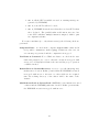
MONFISPOL Grant no.: 225149
Deliverable 2.2.2
Beta-version of parallel routines: user manual.
Marco Ratto, European Commission, Joint Research Centre
Ivano Azzini, Houtan Bastani, Sebastien Villemot, DYNARE Team
July 8, 2011
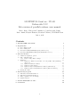
Contents
1 The DYNARE environment
3
2 Requirements
2.1 For a Windows grid . . . . . . . . . . . . . . . . . . . . .
2.2 For a UNIX grid . . . . . . . . . . . . . . . . . . . . . . .
2.3 For hybrid UNIX/WINDOWS grids (UNIX master ) . . .
2.4 For hybrid WINDOWS/UNIX grids (WINDOWS master )
.
.
.
.
.
.
.
.
.
.
.
.
.
.
.
.
.
.
.
.
.
.
.
.
.
.
.
.
.
.
.
.
.
.
.
.
3 The user interface
3.1 Parallel Computation options . . . . . . . . . . . . . . . . . . . . . . . . .
3.2 The configuration file . . . . . . . . . . . . . . . . . . . . . . . . . . . . . .
3.2.1 Preprocessing cluster settings . . . . . . . . . . . . . . . . . . . . .
3.3 Examples . . . . . . . . . . . . . . . . . . . . . . . . . . . . . . . . . . . .
3.3.1 Syntax for Windows and Unix, for local parallel runs (assuming
quad-core) . . . . . . . . . . . . . . . . . . . . . . . . . . . . . . . .
3.3.2 Syntax for Windows clusters . . . . . . . . . . . . . . . . . . . . .
3.3.3 Syntax for Unix clusters . . . . . . . . . . . . . . . . . . . . . . . .
3.3.4 Syntax for hybrid Unix/Windows clusters (Unix master) . . . . . .
3.3.5 Syntax for hybrid Unix/Windows clusters (Windows master) . . .
3.4 Testing the cluster . . . . . . . . . . . . . . . . . . . . . . . . . . . . . . .
4 The
4.1
4.2
4.3
4.4
Developers guide
The function masterParallel.m .
The function fmessageStatus.m .
Write a parallel code: an example .
Synchronization . . . . . . . . . . .
.
.
.
.
.
.
.
.
.
.
.
.
.
.
.
.
.
.
.
.
.
.
.
.
.
.
.
.
.
.
.
.
.
.
.
.
.
.
.
.
.
.
.
.
.
.
.
.
.
.
.
.
.
.
.
.
.
.
.
.
.
.
.
.
.
.
.
.
.
.
.
.
.
.
.
.
.
.
.
.
.
.
.
.
.
.
.
.
.
.
.
.
5
5
5
5
6
7
. 7
. 8
. 11
. 13
.
.
.
.
.
.
13
13
16
17
19
21
.
.
.
.
23
28
29
30
34
5 Parallel DYNARE: test suite
36
6 Conclusions
36
1
Abstract
In this document we describe the parallel package within DYNARE
(called the “Parallel DYNARE” hereafter). The parallel methodology
has been developed taking into account two different perspectives: the
“User perspective” and the “Developers perspective”. The fundamental requirement of the “User perspective” is to allow DYNARE users
to use the parallel routines easily, quickly and appropriately. Under
the “Developers perspective”, on the other hand, we need to build a
core of parallelizing routines that are sufficiently abstract and modular
to allow DYNARE software developers to use them easily as a sort of
‘parallel paradigm’, for application to any DYNARE routine or portion of code containing computational intensive loops suitable for parallelization. The Parallel DYNARE comes with the official DYNARE
installation package, so the preprocessor part required to interpret the
cluster definition is built-in the standard DYNARE installation.
2
1
The DYNARE environment
MATLAB does not allow concurrent programming: it does not support
multi-threads, without the use (and purchase) of MATLAB Distributed
Computing Toolbox. Then, the solution implemented for Parallel DYNARE
can be synthesized as follows:
When the execution of the code should start in parallel, instead
of running it inside the active MATLAB session, the following
steps are performed:
1. the control of the execution is passed to the operating system
(Windows/Linux) that allows for multi-threading;
2. concurrent threads (i.e. MATLAB instances) are launched
on different processors/cores/machines;
3. when the parallel computations are concluded the control is
given back to the original MATLAB session that collects
the result from all parallel ‘agents’ involved and coherently
continue along the sequential computation.
Three core functions have been developed implementing this behavior,
namely MasterParallel.m, slaveParallel.m and fParallel.m. The first
function (MasterParallel.m) operates at the level of the ‘master’ (original) thread and acts as a wrapper of the portion of code to be distributed
in parallel, distributes the tasks and collects the results from the parallel
computation. The other functions (slaveParallel.m and fParallel.m)
operate at the level of each individual ‘slave’ thread and collect the jobs distributed by the ‘master’, execute them and make the final results available
to the master. The two different implementations of slave operation comes
from the fact that, in a single DYNARE session, there may be a number
parallelized sessions that are launched by the master thread. Therefore,
those two routines reflect two different versions of the parallel package:
Open-Close: the ‘slave’ MATLAB sessions are closed after completion of
each single job, and new instances are called for any subsequent parallelized task (fParallel.m);
Always-Open: once opened, the ‘slave’ MATLAB sessions are kept open
during the DYNARE session, waiting for new jobs to be executed,
3
and are only closed upon completion of the DYNARE session on the
‘master’ (slaveParallel.m).
We have seen in the previous report (Deliverable 2.2.1) that none of the
two options is superior to the other, depending on the model size. Namely,
if the model is large and the computations very heavy, the time required to
open new MATLAB instance for every new job is negligible, so the AlwaysOpen mode of execution does not provide a significant reduction in the total
time of the computation with respect to the Open-Close mode. On the other
hand, when the model is not too large, the Always-Open can increase the
speed of the parallel execution.
We have considered the following DYNARE components suitable to be
parallelized using the above strategy:
1. the Random Walk- (and the analogous Independent-)-Metropolis-Hastings
algorithm with multiple chains: the different chains are completely independent and do not require any communication between them, so it
can be executed on different cores/CPUs/Computer Network easily;
2. a number of procedures performed after the completion of Metropolis,
that use the posterior MC sample:
(a) the diagnostic tests for the convergence of the Markov Chain
(McMCDiagnostics.m);
(b) the function that computes posterior IRF’s (posteriorIRF.m).
(c) the function that computes posterior statistics for filtered and
smoothed variables, forecasts, smoothed shocks, etc..
(prior_posterior_statistics.m).
(d) the utility function that loads matrices of results and produces
plots for posterior statistics (pm3.m).
4
2
Requirements
2.1
For a Windows grid
1. a standard Windows network (SMB) must be in place;
2. PsTools (Russinovich, 2009) must be installed in the path of the master
Windows machine;
3. the Windows user on the master machine has to be user of any other
slave machine in the cluster, and that user will be used for the remote
computations.
2.2
For a UNIX grid
1. SSH must be installed on the master and on the slave machines;
2. the UNIX user on the master machine has to be user of any other
slave machine in the cluster, and that user will be used for the remote
computations;
3. SSH keys must be installed so that the SSH connection from the master
to the slaves can be done without passwords, or using an SSH agent.
2.3
For hybrid UNIX/WINDOWS grids (UNIX master )
Here, the same configuration as for standard Unix grid must be in place,
i.e.:
1. SSH must be installed on the master and on the slave Win/Unix machines;
2. the UNIX user on the master machine has to be user of any other
slave machine in the cluster, and that user will be used for the remote
computations;
3. SSH keys must be installed so that the SSH connection from the master
to the Win/Unix slaves can be done without passwords, or using an
SSH agent.
5
2.4
For hybrid WINDOWS/UNIX grids (WINDOWS master )
1. SSH must be installed on the master and on the slave Unix machines;
2. the user on the Windows master machine has to be user of any other
UNIX slave machine in the cluster, and that user will be used for the
remote computations;
3. SSH keys must be installed so that the SSH connection from the master
to the slaves can be done without passwords, or using an SSH agent;
4. for Windows slaves, the same applies as for standard Windows grids.
6
3
The user interface
We assume here that the reader has some familiarity with DYNARE and its
use. For the DYNARE users, the parallel routines are fully integrated and
hidden inside the DYNARE environment.
3.1
Parallel Computation options
Parallel computation will be triggered by the following options passed to the
DYNARE command:
Command line options:
• conffile=<path>: specify the location of the configuration file if it is
not standard ($HOME/.dynare under Unix/Mac, %APPDATA%
dynare.ini under Windows1 );
• parallel: trigger parallel computation using the first cluster specified
in the configuration file;
• parallel=<clustername>: trigger parallel computation, using the
given cluster;
• parallel slave open mode: use the Always-Open mode in the cluster, otherwise the default Open-Close mode is triggered;
• parallel test: just test the cluster, don’t actually run the MOD file;
• console: the console mode is also applicable to the parallel operation,
where all graphical waitbars are replaced by printed information on the
command window.
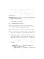
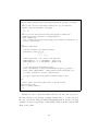
We show in Syntax 1 some examples of DYNARE calls triggering various
parallel options and configurations. We assume that the model file is called
ls2003.mod.
1
c:\Documents and Setting\<username>\Application Data\dynare.ini on XP
7
Standard parallel call (Open-Close mode and configuration file in standard location):
dynare ls2003 parallel
Parallel call with configuration file not in standard location:
dynare ls2003 conffile=’c:\dynare_tests\parallel\JaguarCluster.txt’ parallel
Testing the cluster, using a configuration file named JaguarCluser not placed in the standard
location:
dynare ls2003 conffile=’c:\dynare_tests\parallel\JaguarCluster.txt’ parallel_test
Parallel call with Always-Open mode using the cluster named c2 in the configuration file:
dynare ls2003 parallel=c2 parallel_slave_open_mode
Parallel call with Always-Open mode, console mode and using the cluster named jaguar in
the configuration file:
dynare ls2003 parallel=jaguar parallel_slave_open_mode console
Syntax 1. Examples of various DYNARE parallel calls.
3.2
The configuration file
The general idea is to put all the configuration of the cluster in a config file
different from the MOD file, and to trigger the parallel computation with
option(s) on the dynare command line. The configuration file is designed
as follows:
• allow to specify several clusters, each one associated with a nickname;
• For each cluster, specify a list of slaves with a list of options for each
slave [if not explicitly specified by the configuration file, the preprocessor sets the options to default];
The list of slave options includes:
Name : name of the node;
CPUnbr : this is the number of CPU’s to be used on that computer; if
CPUnbr is a vector of integers, the syntax is [s:d], with d>=s (d, s
are integer); the first core has number 1 so that, on a quad-core, use
4 to use all cores, but use [3:4]to specify just the last two cores (this
8
is particularly relevant for Windows where it is possible to assign jobs
to specific processors);
ComputerName : Computer name on the network or IP address; use the
NETBIOS name under Windows2 , or the DNS name under Unix.;
UserName : required for remote login; in order to assure proper communications between the master and the slave threads, it must be the same
user name actually logged on the ‘master’ machine. On a Windows
network, this is in the form DOMAIN\username, like DEPT\JohnSmith,
i.e. user JohnSmith in windows group DEPT;
Password : required for remote login (only under Windows): it is the user
password on DOMAIN and ComputerName;
RemoteDrive : Drive to be used on remote computer (only for Windows,
for example the drive C or drive D);
RemoteDirectory : Directory to be used on remote computer, the parallel
toolbox will create a new empty temporary subfolder which will act
as remote working directory;
DynarePath : path to matlab directory within the Dynare installation
directory;
MatlabOctavePath : path to MATLAB or Octave executable: note that
hybrid executions using matlab or octave in different machines is allowed (e.g. localhost uses matlab, remote slave uses octave);
SingleCompThread : disable MATLAB’s native multithreading;
OperatingSystem : the operating system of the machine in the cluster:
this is useful for hybrid clusters unix/win and viceversa;
Those options have the specifications shown in Syntax 2.
2
In Windows XP it is possible find this name in ’My Computer’ − > mouse right click
− > ’Property’ − > ’Computer Name’.
9
Node Options
Name
CPUnbr
ComputerName
UserName
Password
RemoteDrive
RemoteDirectory
DynarePath
MatlabOctavePath
SingleCompThread
OperatingSystem
type
example
default
Local
*
*
string
integer
or array
string
Win
Remote
*
*
n1
(stop)
1
(stop)
[2:4]
localhost,
(stop)
karaba.cepremap.org
string
houtanb
empty
string
passwd
empty
string
C
empty
string
/home/houtanb
empty
string
/home/houtanb/
empty
dynare/matlab
string
matlab
empty
boolean
true
true
string
unix
empty
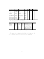
Syntax 2. Configuration file: node options.
Local
*
*
Unix
Remote
*
*
*
*
*
*
*
*
*
*
The cluster options are shown in Syntax 3.
Cluster Options
Name
Members
Members
type
string
string
example
c1
n n2 n3
n4
n(3)
n2(2)
n3(1)
n4(2)
default
empty
empty
Meaning
name of the node
list of members in this
cluster
string
empty
list of members in
this cluster, with their
weights. If no weights
are specified, node use is
distributed evenly.
Syntax 3. Configuration file: cluster options.
Required
*
*
*
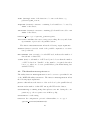
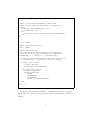
The syntax of the configuration file will take the following form (the
order in which the clusters and nodes are listed is not significant):
10
[cluster]
Name = c1
Members = n1(1) n2(2) n3(2)
[cluster]
Name = c2
Members = n2 n3
[node]
Name = n1
ComputerName = localhost
CPUnbr = 1
[node]
Name = n2
ComputerName = karaba.cepremap.org
CPUnbr = 5
UserName = houtanb
RemoteDirectory = /home/houtanb/Remote
DynarePath = /home/houtanb/dynare/matlab
MatlabOctavePath = matlab
[node]
Name = n3
ComputerName = hal.cepremap.ens.fr
CPUnbr = 3
UserName = houtanb
RemoteDirectory = /home/houtanb/Remote
DynarePath = /home/houtanb/dynare/matlab
MatlabOctavePath = matlab
Example 1. A configuration file.
3.2.1
Preprocessing cluster settings
The DYNARE pre-processor treats user-defined configurations by filling a
dedicated sub-structure in the options_ structure, named parallel. The
structure parallel is a vector, each element corresponding to each node of
the cluster, with the following fields:
11
options_.parallel=
struct(’Local’, Value,
’ComputerName’, Value,
’CPUnbr’, Value,
’UserName’, Value,
’Password’, Value,
’RemoteDrive’, Value,
’RemoteFolder’, Value,
’DynarePath’, Value,
’MatlabOctavePath’, Value,
’OperatingSystem’, Value,
’NodeWeight’, Value,
’SingleCompThread’, Value );
All these fields correspond to the node specifications listed in Syntax 2
except for Local, which is set by the pre-processor according to the value
of ComputerName:
Local: the variable Local is binary, so it can have only two values 0 and 1. If
ComputerName is set to localhost, the preprocessor sets Local = 1
and the parallel computation is executed on the local machine, i.e.
on the same computer (and working directory) where the DYNARE
project is placed. For any other value for ComputerName, we will have
Local = 0;
In addition to the parallel structure there is another options_ field,
called parallel_info, which stores all options that are common to all cluster.
options_.parallel_info=
struct(’leaveSlaveOpen’, Value,
’RemoteTmpFolder’, Value);
In particular, according to the parallel_slave_open_mode in the command line, the parallel_info.leaveSlaveOpen field takes values:
leaveSlaveOpen=1 : with parallel_slave_open_mode, i.e. the slaves operate ‘Always-Open’.
leaveSlaveOpen=0 : without parallel_slave_open_mode, i.e. the slaves
operate ‘Open-Close’;
12
Moreover, when the parallel computations are done on a remote machine, the
field parallel_info.RemoteTmpFolder stores the name of the temporary
subdirectory which acts as the working directory of the remote computations. In fact, to avoid possible erroneous overwriting or deletion of the
information stored on the disks of the remote machine, the remote working
directory is not directly the one specified in parallel.RemoteFolder, but
it is a new, empty, temporary subdirectory, whose name is generated according to the date and time when the parallel computations are initialized.
For example, a typical temporary directory name is
parallel_info.RemoteTmpFolder=2011-7-7-12h43m7s
and, assuming parallel.RemoteFolder=’/home/houtan’, the full path to
the remote working directory will thus be /home/houtan/2011-7-7-12h43m7s.
3.3
3.3.1
Examples
Syntax for Windows and Unix, for local parallel runs (assuming quad-core)
In this case, the only slave options are ComputerName and CPUnbr.
[cluster]
Name = local
Members = n1
[node]
Name = n1
ComputerName = localhost
CPUnbr = 4
Example 2. Local parallel configuration.
3.3.2
Syntax for Windows clusters
• the Windows Password has to be typed explicitly;
• RemoteDrive has to be typed explicitly;
• for UserName, ALSO the group has to be specified, like DEPT\JohnSmith,
i.e. user JohnSmith in windows group DEPT;
• ComputerName is the name of the computer in the windows network,
i.e. the output of hostname, or the full IP address.
13
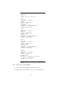
In Example 3, parallel codes are run on a remote computer named
vonNeumann with eight cores, using only the cores 4,5,6, working on the
drive ’C’ and folder ’dynare_calcs\Remote’. The computer vonNeumann is
in a net domain of the CompuTown university, with user John logged with
the password *****.
[cluster]
Name = vonNeumann
Members = n2
[node]
Name = n2
ComputerName = vonNeumann
CPUnbr = [4:6]
UserName = COMPUTOWN\John
Password = *****
RemoteDrive = C
RemoteDirectory = dynare_calcs\Remote
DynarePath = c:\dynare\matlab
MatlabOctavePath = matlab
Example 3. Remote parallel configuration.
We can build clusters, combining local and remote runs. In Example 4,
the configuration file includes the two previous configurations but also gives
the possibility (with cluster name c2) to build a grid with a total number
of 7 CPU’s and where the remote vonNeumann machine has a double weight
with respect to the local machine.
14
[cluster]
Name = local
Members = n1
[cluster]
Name = vonNeumann
Members = n2
[cluster]
Name = c2
Members = n1(1) n2(2)
[node]
Name = n1
ComputerName = localhost
CPUnbr = 4
[node]
Name = n2
ComputerName = vonNeumann
CPUnbr = [4:6]
UserName = COMPUTOWN\John
Password = *****
RemoteDrive = C
RemoteDirectory = dynare_calcs\Remote
DynarePath = c:\dynare\matlab
MatlabOctavePath = matlab
Three types of clusters can be called, using the same
configuration file, using the different DYNARE command
line options:
dynare ls2003 parallel=local
dynare ls2003 parallel=vonNeumann
dynare ls2003 parallel=c2
Example 4. Windows: configuration of a cluster (local
and remote executions).
We can build a cluster, combining many remote machines, as in Example
5 where we build a grid of four machines with a total number of 14 CPU’s.
15
[cluster]
Name = c4
Members = n1(1) n2(2) n3(3) n4(3)
[node]
Name = n1
ComputerName = vonNeumann1
CPUnbr = 4
UserName = COMPUTOWN\John
Password = *****
RemoteDrive = C
RemoteDirectory = dynare_calcs\Remote
DynarePath = c:\dynare\matlab
MatlabOctavePath = matlab
[node]
Name = n2
ComputerName = vonNeumann2
CPUnbr = 4
UserName = COMPUTOWN\John
Password = *****
RemoteDrive = C
RemoteDirectory = dynare_calcs\Remote
DynarePath = c:\dynare\matlab
MatlabOctavePath = matlab
[node]
Name = n3
ComputerName = vonNeumann3
CPUnbr = 2
UserName = COMPUTOWN\John
Password = *****
RemoteDrive = D
RemoteDirectory = dynare_calcs\Remote
DynarePath = c:\dynare\matlab
MatlabOctavePath = matlab
[node]
Name = n4
ComputerName = vonNeumann4
CPUnbr = 4
UserName = COMPUTOWN\John
Password = *****
RemoteDrive = C
RemoteDirectory = John\dynare_calcs\Remote
DynarePath = c:\dynare\matlab
MatlabOctavePath = matlab
Example 5. Windows: configuration of a cluster (remote executions).
3.3.3
Syntax for Unix clusters
• no Password and RemoteDrive fields are needed;
• ComputerName is the full IP address or the DNS address.
16
In the case of one remote slave, Example 6 defines remote runs on the
machine name.domain.org.
[cluster]
Name = unix1
Members = n2
[node]
Name = n2
ComputerName = name.domain.org
CPUnbr = 4
UserName = JohnSmith
RemoteDirectory = /home/john/Remote
DynarePath = /home/john/dynare/matlab
MatlabOctavePath = matlab
Example 6. Unix: configuration for remote executions.
We can combine local and remote runs, as in Example 7.
[cluster]
Name = unix2
Members = n1 n2
[node]
Name = n1
ComputerName = localhost
CPUnbr = 4
[node]
Name = n2
ComputerName = name.domain.org
CPUnbr = 4
UserName = JohnSmith
RemoteDirectory = /home/john/Remote
DynarePath = /home/john/dynare/matlab
MatlabOctavePath = matlab
Example 7. Unix: configuration for local and remote
executions.
3.3.4
Syntax for hybrid Unix/Windows clusters (Unix master)
• unix machines in the cluster follow the same rules as for standard Unix
clusters;
17
• for windows machines the field ComputerName is the full IP address
or the DNS address (i.e. no longer the NETBIOS in the Windows
network);
• for windows machines the field UserName is the user name for the unix
machine, no longer the GROUP\username of the windows network;
• for windows machines the field OperatingSystem must be set equal to
’windows’;
• SSH must be installed on the remote windows machines, and SSH keys
have to be installed such that the unix master is allowed to connect to
the remote Windows without password or through an SSH agent (so
also for windows machines the field Password can be left empty).
In Example 8, the unix master uses a remote windows machine, while in
Example 9 it uses both unix and windows machines. Also note the hybrid
matlab/octave computations in the latter cluster.
[cluster]
Name = hybrid1
Members = n1 n2
[node]
Name = n1
ComputerName = localhost
CPUnbr = 4
[node]
Name = n4
ComputerName = vonNeumann4.computown.org
CPUnbr = 4
UserName = John
RemoteDrive = C
RemoteDirectory = John\dynare_calcs\Remote
DynarePath = c:\dynare\matlab
MatlabOctavePath = matlab
OperatingSystem = windows
Example 8. Unix master combined with remote windows
executions.
18
[cluster]
Name = hybrid2
Members = n1(2) n2(1) n4(2)
[node]
Name = n1
ComputerName = localhost
CPUnbr = 4
[node]
Name = n2
ComputerName = name.domain.org
CPUnbr = 4
UserName = JohnSmith
RemoteDirectory = /home/john/Remote
DynarePath = /home/john/dynare/matlab
MatlabOctavePath = octave
OperatingSystem = unix
[node]
Name = n4
ComputerName = vonNeumann4.computown.org
CPUnbr = 4
UserName = John
RemoteDrive = C
RemoteDirectory = John\dynare_calcs\Remote
DynarePath = c:\dynare\matlab
MatlabOctavePath = matlab
OperatingSystem = windows
Example 9. Windows master combined with remote
unix/windows executions.
3.3.5
Syntax for hybrid Unix/Windows clusters (Windows master)
• unix machines in the cluster follow the same rules as for standard Unix
clusters;
• for unix machines the field OperatingSystem must be set equal to
’unix’;
• windows machines in the cluster follow the same rules as for standard
Windows clusters;
• SSH must be installed on the master windows machine, and SSH keys
19
have to be installed such that the windows master is allowed to connect
to the remote unix machines without password or through an SSH
agent.
In Example 10 we show the case of a Windows master performing local
executions and remote executions on a unix machine, while in Example 11
remote machines are both unix and windows. Moreoever, the remote unix
machine does not have a MATLAB license, so octave is used instead, so we
assume that matlab executions have double weight with respect to octave
ones.
[cluster]
Name = hybrid3
Members = n1(2) n2(1)
[node]
Name = n1
ComputerName = localhost
CPUnbr = 4
[node]
Name = n2
ComputerName = name.domain.org
CPUnbr = 4
UserName = JohnSmith
RemoteDirectory = /home/john/Remote
DynarePath = /home/john/dynare/matlab
MatlabOctavePath = octave
OperatingSystem = unix
Example 10. Windows master combined with remote
unix executions.
20
[cluster]
Name = hybrid4
Members = n1(2) n2(1) n4(2)
[node]
Name = n1
ComputerName = localhost
CPUnbr = 4
[node]
Name = n2
ComputerName = name.domain.org
CPUnbr = 4
UserName = JohnSmith
RemoteDirectory = /home/john/Remote
DynarePath = /home/john/dynare/matlab
MatlabOctavePath = octave
OperatingSystem = unix
[node]
Name = n4
ComputerName = vonNeumann4
CPUnbr = 4
UserName = COMPUTOWN\John
Password = *****
RemoteDrive = C
RemoteDirectory = John\dynare_calcs\Remote
DynarePath = c:\dynare\matlab
MatlabOctavePath = matlab
Example 11. Windows master combined with remote
unix/windows executions.
3.4
Testing the cluster
In this section we describe the testing routine that checks if the cluster
defined in the configuration file works properly. In parallel DYNARE there
is a utility (AnalyseComputationalEnvironment.m) devoted to this task
(this is triggered by the command line option parallel_test).
For both local and remote machines, the following checks are performed:
CPUnbr: the value for this variable is in the form [s:d] or simply d:
the testing routine checks if d CPUs (or cores) are available on the
computer. Suppose that this check returns an integer nC. We can have
three possibilities:
21
1. nC= d; all the CPU’s available are used, no warning message are
generated by DYNARE;
2. nC> d; some CPU’s will not be used;
3. nC< d; DYNARE alerts the user that there are less CPU’s than
those declared. The parallel tasks would run in any case, but
some CPU’s will have multiple instances assigned, with no gain
in computational time.
For remote machines (i.e. only when Local=0), the following check are
performed:
ComputerName : we check if the computer ComputerName exists and if
it is possible communicate with it (ping). If this is not the case, an
error message is generated and the computation is stopped.
UserName & Password: For a Windows cluster, we check if the user
name and password are correct, otherwise execution is stopped with
an error; for a Unix/hybrid cluster, the user and the proper operation
of SSH is checked.
RemoteDrive & RemoteDirectory: we try to copy a file (Tracing.txt)
in this remote location. If this operation fails, the DYNARE execution
is stopped with an error. if Local = 1, these fields are not required
since the working directory of the ‘slaves’ will be the same of the
‘master’.
MatlabOctavePath & DynarePath: MATLAB/octave instances are tried
on slaves and the DYNARE path is also checked. If this operation fails,
the DYNARE execution is stopped with an error.
22
4
The Developers guide
In this section we describe with some accuracy the DYNARE parallel routines.
Windows: With Windows operating system, the parallel package requires
the installation of a free software package called PsTools (Russinovich,
2009). PsTools suite is a resource kit with a number of command line
tools that mimics administrative features available under the Unix
environment. PsTools can be downloaded from
http://technet.microsoft.com/en-us/sysinternals/bb896649.aspx
and extracted in a Windows directory on your computer: to make
PsTools working properly, it is mandatory to add this directory to
the Windows path. After this step it is possible to invoke and use
the PsTools commands from any location in the Windows file system. PsTools, MATLAB and DYNARE have to be installed and work
properly on all the machines in the grid for parallel computation.
Unix: With Unix operating system, SSH must be installed on the master
and on the slave machines. Moreover, SSH keys must be installed so
that the SSH connections from the master to the slaves can be done
without passwords or using an SSH agent.
Hybrid Unix/Win grids: the parallel operation for hybrid grids, where
machines can have different operating systems, is done via the SSH
protocol. So, the latter also has to be installed on the Windows machines as for a standard Unix grid. The SSH protocol is available for
Windows either with cygwin or openSSH.
As soon as the computational environment is set-up for working on a
grid of CPU’s, the parallel package allows to parallelize any loop that is
computationally expensive, following the step by step procedure showed
in Table 1. This is done using five basic functions: masterParallel.m,
fParallel.m or slaveParallel.m, fMessageStatus.m, closeSlave.m.
masterParallel is the entry point to the parallelization system:
• It is called from the master computer, at the point where the parallelization system should be activated. Its main arguments are
23
the name of the function containing the task to be run on every
slave computer, inputs to that function stored in two structures
(one for local and the other for global variables), and the configuration of the cluster; this function exits when the task has
finished on all computers of the cluster, and returns the output
in a structure vector (one entry per slave);
• all file exchange through the filesystem is concentrated in this
masterParallel routine: so it prepares and send the input information for slaves, it retrieves from slaves the info about the
status of remote computations stored on remote slaves by the
remote processes; finally it retrieves outputs stored on remote
machines by slave processes;
• there are two modes of parallel execution, triggered by option
parallel_slave_open_mode:
– when parallel_slave_open_mode=0, the slave processes are
closed after the completion of each task, and new instances
are initiated when a new job is required; this mode is managed by fParallel.m [‘Open-Close’];
– when parallel_slave_open_mode=1, the slave processes are
kept running after the completion of each task, and wait
for new jobs to be performed; this mode is managed by
slaveParallel.m [‘Always-Open’];
slaveParallel.m/fParallel.m: are the top-level functions to be run on
every slave; their main arguments are the name of the function to be
run (containing the computing task), and some information identifying
the slave; the functions use the input information that has been previously prepared and sent by masterParallel through the filesystem,
call the computing task, finally the routines store locally on remote
machines the outputs such that masterParallel retrieves back the
outputs to the master computer;
fMessageStatus.m: provides the core for simple message passing during
slave execution: using this routine, slave processes can store locally on
remote machine basic info on the progress of computations; such information is retrieved by the master process (i.e. masterParallel.m)
24
allowing to echo progress of remote computations on the master; the
routine fMessageStatus.m is also the entry-point where a signal of
interruption sent by the master can be checked and executed; this
routine typically replaces calls to waitbar.m;
closeSlave.m is the utility that sends a signal to remote slaves to close
themselves. In the standard operation, this is only needed with the
‘Always-Open’ mode and it is called when DYNARE computations
are completed. At that point, slaveParallel.m will get a signal to
terminate and no longer wait for new jobs. However, this utility is
also useful in any parallel mode if, for any reason, the master needs to
interrupt the remote computations which are running;
The parallel toolbox also includes a number of utilities:
• AnalyseComputationalEnviroment.m: this a testing utility that checks
that the cluster works properly and echoes error messages when problems are detected;
• InitializeComputationalEnviroment.m : initializes some internal
variables and remote directories;
• distributeJobs.m: uses a simple algorithm to distribute evenly jobs
across the available CPU’s;
• a number of generalized routines that properly perform delete, copy,
mkdir, rmdir commands through the network file-system (i.e. used
from the master to operate on slave machines); the routines are adaptive to the actual environment (Windows or Unix);
dynareParallelDelete.m : generalized delete;
dynareParallelDir.m : generalized dir;
dynareParallelGetFiles.m : generalized copy FROM slaves TO
master machine;
dynareParallelMkDir.m : generalized mkdir on remote machines;
dynareParallelRmDir.m : generalized rmdir on remote machined;
dynareParallelSendFiles.m : generalized copy TO slaves FROM
master machine;
25
• a number of utilities that allow the master to retrieve files generated by
remote machines on-the-fly, i.e. as soon as they are available without
waiting that the entire remote thread is finished:
dynareParallelFindNewFiles.m : on-the-fly list new files saved by
remote machines;
dynareParallelGetNewFiles.m : on-the-fly copy new files FROM
remote TO master machine;
dynareParallelSnapshot.m : snapshot of all files present in the remote working directory;
In Table 1 we have synthesized the main steps for parallelizing MATLAB
codes.
So far, we have parallelized the following functions, by selecting the most
computationally intensive loops:
1. the cycle looping for multiple chain random walk Metropolis:
random_walk_metropolis_hastings,
random_walk_metropolis_hastings_core;
2. the cycle looping for multiple chain independent Metropolis:
independent_metropolis_hastings.m,
independent_metropolis_hastings_core.m;
3. the cycle looping over estimated parameters computing univariate diagnostics:
McMCDiagnostics.m,
McMCDiagnostics_core.m;
4. the Monte Carlo cycle looping over posterior parameter subdraws performing the IRF simulations (<*>_core1) and the cycle looping over
exogenous shocks plotting IRF’s charts (<*>_core2):
posteriorIRF.m,
posteriorIRF_core1.m, posteriorIRF_core2.m;
5. the Monte Carlo cycle looping over posterior parameter subdraws, that
computes filtered, smoothed, forecasted variables and shocks:
prior_posterior_statistics.m,
prior_posterior_statistics_core.m;
26
1. locate within DYNARE the portion of code suitable to be parallelized,
i.e. an expensive cycle for;
2. suppose that the function tuna.m contains a cycle for that is suitable
for parallelization: this cycle has to be extracted from tuna.m and put
it in a new MATLAB function named tuna_core.m;
3. at the point where the expensive cycle should start, the function
tuna.m invokes the utility masterParallel.m, passing to it the
options_.parallel structure, the name of the of the function to be
run in parallel (tuna_core.m), the local and global variables needed
and all the information about the files (MATLAB functions *.m; data
files *.mat) that will be handled by tuna_core.m;
4. the function masterParallel.m reads the input arguments provided
by tuna.m and:
• decides how to distribute the task evenly across the available CPU’s (using the utility routine distributeJobs.m); prepares and initializes the computational environment (i.e. copy
files/data) for each slave machine;
• uses the PsTools and the Operating System commands to launch
new MATLAB instances, synchronize the computations, monitor
the progress of slave tasks through a simple message passing system (see later) and collect results upon completion of the slave
threads;
5. the slave threads are executed using the MATLAB functions
fParallel.m/slaveParallel.m as wrappers for implementing the
tasks sent by the master (i.e. to run the tuna_core.m routine);
6. the utility fMessageStatus.m can be used within the core routine
tuna_core.m to send information to the master regarding the progress
of the slave thread;
7. when all DYNARE computations are completed, closeSlave.m closes
all open remote MATLAB/OCTAVE instances waiting for new jobs
to be run.
Table 1: Procedure for parallelizing portions of codes.
27
6. the cycle looping over endogenous variables making posterior plots of
filter, smoother, forecasts: pm3.m, pm3_core.m.
Essentially, developers need to interface with only two of the above mentioned functions: masterParallel.m and fmessageStatus.m. All other
functions act as internal functions and knowing their usage is not necessary
for the developer.
function masterParallel.m is used to break the serial computation and
initiate parallel implementation;
function fmessageStatus.m is used in parallel threads to send information
about the status of computations.
4.1
The function masterParallel.m
The function masterParallel.m has the following input arguments:
Parallel (struct vector): copy of options_.parallel, i.e. the vector
of structures describing each machine in the cluster;
fBlock (int): index number of the first thread (between 1 and nBlock);
nBlock (int): index number of the last thread: the loop [fBLock:nBLock]
will be broken and distributed across all available CPU’s in the cluster;
NamFileInput (cell array): contains the list of input files to be copied
in the working directory of remote slaves. It is made of 2 columns,
with as many lines as there are files (i) first column contains directory
paths relative to the remote working directory (i.e. if the files have to
be moved to the remote working directory, the entry in the first column
will be an empty string!) (ii) second column contains filenames (e.g.
<model>_static.m, <model>_dynamic.m, <model>_steadystate.m),
for exmple:
NamFileInput(1,:) = {’’,[ModelName ’_static.m’]};
NamFileInput(2,:) = {’’,[ModelName ’_dynamic.m’]};
if options_.steadystate_flag,
NamFileInput(3,:)={’’,[ModelName ’_steadystate.m’]};
end
28
fname (string): name of the function to be run on the slaves, e.g.
posterior_IRF_core.m;
fInputVar (struct): structure containing local variables to be used by
fName on the slaves;
fGlobalVar (struct): structure containing global variables needed to run
fName on the slaves;
Parallel info: copy of options_.parallel_info;
initialize: initializes the remote temporary working directory and cleans
up remnants of previous local parallel sessions.
The function masterParallel.m has the following output arguments:
fOutVar (struct vector): result of the parallel computation, one structure per thread;
nBlockPerCPU (int vector): for each CPU used, indicates the number of
threads run on that CPU;
totCPU (int): total number of CPU used (can be lower than the number
of CPU declared in ”Parallel”, if the number of required threads is
lower, e.g. when one does two parallel Metropolis chains having four
available CPU’s).
4.2
The function fmessageStatus.m
The utility function fMessageStatus.m can be seen as a generalized form
of the MATLAB utility waitbar.m. The function fMessageStatus.m has
the following input arguments:
prtfrc: this indicates the fraction of the work done by the parallel thread;
whoiam: index number of this CPU among all CPUs in the cluster;
waitbarString: a running string that updates some info during the computation (e.g. the acceptance rate in Metropolis);
waitbarTitle: a title string;
Parallel: the configuration options for this machine, i.e. a copy of
options .parallel(ThisMatlab).
29
4.3
Write a parallel code: an example
Using a MATLAB pseudo (but very realistic) code, we now describe in detail how to use the above step by step procedure to parallelize the random
walk Metropolis Hastings algorithm. Any other function can be parallelized
in the same way. It is obvious that most of the computational time spent
by the
random_walk_metropolis_hastings.m function is given by the cycle looping over the parallel chains performing the Metropolis:
function random_walk_metropolis_hastings
(TargetFun, ProposalFun, ..., varargin)
[...]
for b = fblck:nblck,
...
end
[...]
Since those chains are totally independent, the obvious way to reduce the
computational time is to parallelize this loop, executing the (nblck-fblck)
chains on different computers/CPUs/cores.
To do so, we remove the for cycle and put it in a new function named
<*>_core.m:
30
function myoutput =
random_walk_metropolis_hastings_core(myinputs,fblck,nblck, ...)
[...]
just list global variables needed (they are set-up properly by fParallel or slaveParallel)
global bayestopt_ estim_params_ options_
M_ oo_
here we collect all local variables stored in myinputs
TargetFun=myinputs.TargetFun;
ProposalFun=myinputs.ProposalFun;
xparam1=myinputs.xparam1;
[...]
here we run the loop
for b = fblck:nblck,
...
end
[...]
here we wrap all output arguments needed by the ‘master’ routine
myoutput.record = record;
[...]
The split of the for cycle has to be performed in such a way that the new
<*>_core function can work in both serial and parallel mode. In the latter
case, such a function will be invoked by the slave threads and executed for
the number of iterations assigned by masterParallel.m.
The modified random_walk_metropolis_hastings.m is therefore:
31
function random_walk_metropolis_hastings(TargetFun,ProposalFun,,varargin)
[...]
% here we wrap all local variables needed by the <*>_core function
localVars = struct(’TargetFun’, TargetFun, ...
[...]
’d’, d);
[...]
% here we put the switch between serial and parallel computation:
if isnumeric(options_.parallel) || (nblck-fblck)==0,
% serial computation
fout = random_walk_metropolis_hastings_core(localVars, fblck,nblck, 0);
record = fout.record;
else
% parallel computation
% global variables for parallel routines
globalVars = struct(’M_’,M_, ...
[...]
’oo_’, oo_);
% which files have to be copied to run remotely
NamFileInput(1,:) = {’’,[ModelName ’_static.m’]};
NamFileInput(2,:) = {’’,[ModelName ’_dynamic.m’]};
[ ...]
% call the master parallelizing utility
[fout, nBlockPerCPU, totCPU] = masterParallel(options_.parallel, ...
fblck, nblck, NamFileInput, ’random_walk_metropolis_hastings_core’,
localVars, globalVars, options_.parallel_info);
% collect output info from parallel tasks provided in fout
[ ...]
end
% collect output info from either serial or parallel tasks
irun = fout(1).irun;
NewFile = fout(1).NewFile;
[...]
Finally, in order to allow the master thread to monitor the progress of
the slave threads, some message passing elements have to be introduced in
the <*>_core.m file, using the utility fMessageStatus.m. In the following
example, we show a typical use of this utility, again from the random walk
Metropolis routine:
32
[...]
% define a title message waitbarTitle, common for the
% entire execution (typically which machine is doing the job)
if whoiam
if options_.parallel(ThisMatlab).Local,
waitbarTitle=[’Local ’];
else
waitbarTitle=[options_.parallel(ThisMatlab).ComputerName];
end
end
[...]
for j = 1:nruns
[...]
% define the progress of the loop:
prtfrc = j/nruns;
% define a running message:
% first indicate which chain is running on the current CPU [b]
% out of the chains [mh_nblock] requested by the DYNARE user
waitbarString = [ ’(’ int2str(b) ’/’ int2str(mh_nblck) ’) ...
% then add possible further information, like the acceptation rate
’ sprintf(’%f done, acceptation rate %f’,prtfrc,isux/j)]
if mod(j, 3)==0 & ~whoiam
% serial computation
waitbar(prtfrc,hh,waitbarString);
elseif mod(j,50)==0 & whoiam,
% parallel computation
fMessageStatus(prtfrc, ...
whoiam, ...
waitbarString, ...
waitbarTitle, ...
options_.parallel(ThisMatlab))
end
[...]
end
In the previous example, a number of arguments are used to identify
which CPU and which computer in the cluster is sending the message,
namely:
33
%
%
%
%
whoiam [int]
ThisMatlab [int]
index number of this CPU among all CPUs in the
cluster
index number of this slave machine in the cluster
(entry in options_.parallel)
The message is stored as a MATLAB data file
[’comp_status_’,fname,’*.mat’]
saved on the working directory of remote slave computer. The master will
will check periodically for those messages and retrieve the files from remote
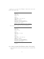
computers and produce an advanced monitoring plot.
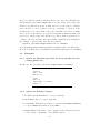
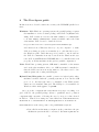
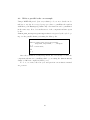
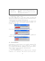
So, assuming to run two Metropolis chains, under the standard serial
implementation there will be a first waitbar popping up on matlab, corresponding to the first chain:
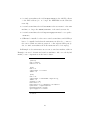
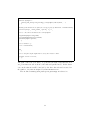
followed by a second waitbar, when the first chain is completed.
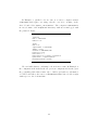
On the other hand, under the parallel implementation, a parallel monitoring plot will be produced by masterParallel.m:
4.4
Synchronization
Synchronization is a critical element for proper parallel computations. The
function masterParallel needs to wait for all threads to be completed
before wrapping up all results and continuing the serial execution. Synchronization is assure creating/deleting files: namely files named
[’P_’,fname,’_*End.txt’]
are created by masterParallel in the working directories of all parallel threads, one for each thread. Those files are deleted by the remote
34
threads as their last instruction after completion of all required tasks. Then
masterParallel waits until all files [’P_’,fname,’_*End.txt’] are deleted
before proceeding further. In practice, masterParallel does two operations
while parallel threads are running:
1. checks every second the status of remote computations, i.e. looks for
files named
[’comp_status_’,fname,’*.mat’]
saved by fmessageStatus.m;
2. checks that all threads are completed, i.e. deletion of all files
[’P_’,fname,’_*End.txt’].
In the case of the ”Always-Open” mode, further synchronization is needed
for the function slaveParallel.m having to wait for new jobs arriving. New
jobs are sent by masterParallel.m by means of a file
[’slaveJob’,int2str(whoiam),’.mat’]
which stores all info about the thread to be run. So, slaveParallel.m waits
and checks the existence of such files every second. When this file is on the
working directory, new threads are started. In order to avoid that remote
MATLAB instances stay open forever (e.g. in the case master crashes for
some reason), the remote MATLAB closes after 1200 seconds without any
new request. The master can reset the counter of 1200 seconds by sending
a file named
[’stayalive’,int2str(whoiam),’.txt’]
to the remote working directory: slaves check for the existence of such a file,
if it exist the counter is reset to zero and the file deleted. The master can
impose the remote MATLAB to close at any time by deleting files named
[’slaveParallel_input’,int2str(whoiam),’.mat’]
(the closeSlave.m utility does this operation). Remote slaves check periodically the existence of such files and if they are deleted they exit MATLAB.
The existence of such files is also checked by fmessageStatus whenever it
is invoked by the _core routine: in this way, a signal of breaking remote
execution can be sent also inside computational threads.
35
5
Parallel DYNARE: test suite
We provide in the official DYNARE distribution tests for parallel execution
(tests/parallel subfolder).
6
Conclusions
The parallel DYNARE is built around a few ‘core’ routines, that act as a
sort of ‘parallel paradigm’. Based on those routines, parallelization of expensive loops is made quite simple for DYNARE developers. A basic message
passing system is also provided, that allows the master thread to monitor
the progress of slave threads. The test model ls2003.mod is available in the
folder \tests\parallel of the DYNARE distribution, that allows running
parallel examples.
References
M. Russinovich.
PsTools v2.44, 2009.
available at Microsoft TechNet,
http://technet.microsoft.com/en-us/sysinternals/bb896649.aspx.
36