Download GiD

GiD
THE PERSONAL PRE
AND POSTPROCESSOR
The universal, adaptive and user
friendly pre and post processing
system for computer analysis
in science and engineering
User Manual
Version 8
Developers
Ramon Ribó
Miguel de Riera Pasenau
Enrique Escolano
Jorge Suit Pérez Ronda
Abel Coll Sans
Cover design
Lluis Font González
For further information please contact
International Center for Numerical Methods in Engineering
Edificio C1, Campus Norte UPC
Gran Capitán s/n, 08034 Barcelona, Spain
http://www.gidhome.com
gid@cimne.upc.edu
Depósito legal:B-34.736-02
ISBN User Manual: 84-95999-94-3
ISBN Obra Completa: 84-95999-96-x
© CIMNE (Barcelona, Spain)
TABLE OF CONTENTS
Presentation of GiD……………………………………………………………………………………. 1
Initiation to GiD……………………………………………………………………………………….. 23
Case study 1: implementing a mechanical part…………………………………………………... 42
Case study 2: implementing a cooling pipe……………………………………………………….. 73
Assigning element sizes for generation the mesh………………………………………………... 96
Methods for generating the mesh……………………………………………………………….… 111
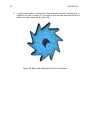
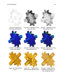
A postprocess case study: postprocessing a ratchet wheel………………………………….…128
Importing files: a case study………………………………………………………………………...160
Defining a problem type……………………………………………………………………………..183
GID USER MANUAL
1
PRESENTATION OF GID
This chapter will introduce the user to the user-interface and graphic environment of GiD.
GiD is a general purpose pre-postprocessor for computer analysis.
All the data, geometry and mesh generation can be performed inside. Also, the visualization of
all types of results can be performed.
It can be adapted to a specific analysis module by the creation of a 'problem type'.
Typical problems that can be successfully tackled with GiD include most situations in solid and
structural mechanics, fluid dynamics, electromagnetics, heat transfer, geomechanics, etc. using
finite element, finite volume, boundary element, finite difference or point based (meshless)
numerical procedures.
2
PRESENTATION OF GID
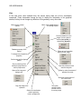
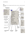
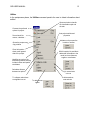
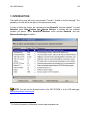
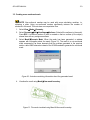
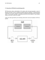
USER INTERFACE
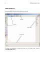
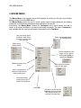
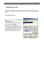
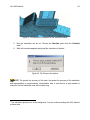
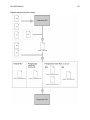
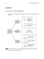
Upon opening GiD, the following window appears on the screen:
Top menu
Toolbars
Right buttons
Command line
To change the configuration of toolbars and menus, use the toolbars option, located in
UtilitiesÆToolsÆToolbars.
GID USER MANUAL
3
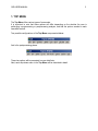
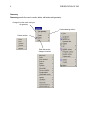
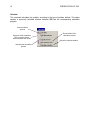
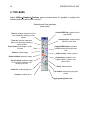
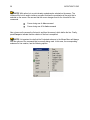
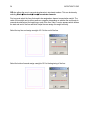
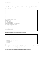
1. TOP MENU
The Top Menu offers various types of commands.
It is important to note that these options will differ depending on the whether the user is
performing a preprocessing or postprocessing analysis, and that the options needed in each
case differ as well.
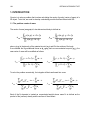
Two possible configurations of the Top Menu are presented below:
And in the postprocessing phase:
These two options will be presented in more detail later.
Next, each drop-down menu in the Top Menu will be described in detail.
4
PRESENTATION OF GID
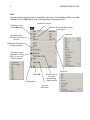
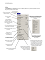
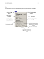
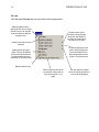
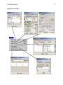
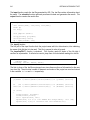
Files
Two main types of functions can be controlled in this menu: 1) the handling of files (i.e. create,
read, save, etc.) of GiD projects; and, 2) the importing and exporting of files.
Creates a new project
Reads a previously
created GiD project
Saves to disc all information related
to the project
Import files
Saves information
with name chosen by
the user
Changes the configuration for
postprocess phase
Saves the drawing
image shown on the
screen, in one of the
following formats
Export files
Closes GiD
Printing options
Window to set up
some print
properties and
image properties
Open the
last models
GID USER MANUAL
5
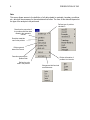
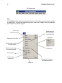
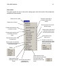
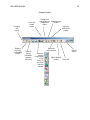
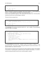
View
In the view menu (also available from the mouse menu) there are all the visualization
commands. These commands change the way to display the information in the graphical
window, but they do not change any definition of the geometry or any other data.
Offers various rotation
options:
Offers various zoom options
for viewing of piece
Permits translations of the
image, from one point to
another (two points), or
dynamically (dynamic)
Redraws geometry of the
project
To change to a perspective
projection
Offers various illumination
options for the image
Set the near and far clipping
planes
Show numbering of the
entities for preprocess as
well for postprocess
Draw the surfaces normal
sans line tangents
Opens a file image as a
background
Draw by colors the amount of
parents of an entity
Saves the actual position of
the current view
Copy the image to the
clipboard
Switch the visualization
mode to geometry
mesh or postprocess
This option
permits to have
several views of
the same project
6
PRESENTATION OF GID
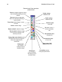
Geometry
Geometry permits the user to create, delete, edit and model geometry.
Changes from the mesh viewing to
the geometry
Creates drawing entities
Deletes entities
Edits and permits
changes to entities
GID USER MANUAL
7
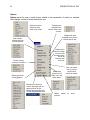
Utilities
In the Utilities menu, GiD allows the user to define preferences or perform operations on both
the geometry and the mesh entities.
Chooses the preferred
options for project
Undo commands
executed during the work
session
Opens the layers
window
GiD is flexible in its configuration of the
screen and accommodates different
menus depending on the user’s
preference
Moves entities as
translation, rotation,
symmetry, scale, in this
case without duplicating
entities
Gives information about useful
general data of the project
Lists project entities and
properties
Shows labels and
coordinates of new
or existing points
Copies all types of entities by
performing a translation,
rotation, mirror symmetry or
entity scaling
Indicates on the screen the
location of entities
Manage the orientation of
the entity normal
Renumbers the entity labels, in order
to avoid gaps in numbering caused
by the elimination of entities during
the description of geometry and its
properties. Renumbers the mesh to
decrease the analysis interval
Calculates the distance
between points
Checks the internal coherence
of the data base
With this option it's possible to
add textual information to the
model, such as distances,
angles or coordinates.
8
PRESENTATION OF GID
Data
This menu allows access to the definition of all data related to materials, boundary conditions,
etc., which will be necessary for the calculations that follow. The form of this data will depend on
the type of the analysis to be performed.
Defines type of problem
calculation
Describes the properties of
the problem and other data
related to the geometric
entities
Describes materials
used in the problem
Defines general
data of the interval
Describes generally the
problem data
Defines the units
used in the problem
Divides information of
problem into intervals
Changes and defines local
coordinate axes
GID USER MANUAL
9
Mesh
Mesh permits the user to generate and edit the mesh, as well as to select mesh creation
preferences.
Defines a structured
mesh
Assigns element sizes
to entities for non
structured mesh
Defines a semi
structured mesh
Describes element
type to be used
Chooses default mesh
criteria, meshing of
determined entities or
not of others
Deletes assigned
information for mesh
generation
Assign element
type to entities
Draw in different
colors the different
mesh information
Generates the mesh
Shows
boundaries
of meshing
process
Cancels previously
generated mesh
Open the window with
the last meshing error
message
Shows quality of
mesh elements
generated
Create
boundaries
of meshing
process
Edits and permits
changes to the mesh
10
PRESENTATION OF GID
Calculate
This command calculates the problem, according to the type of problem defined. This option
requires a previously activated interface between GiD and the corresponding calculation
program.
Start calculation
process
Sends the mesh created by
GiD to a remote server,
which calculates the results
Interrupts the calculation
process
Shows details of the
calculation process
Opens the calculate window
GID USER MANUAL
11
Help
This menu permits the user to obtain different types of help and information about GiD.
Interactive help
covering all GiD
options
What is new in
this version
Use this option to
register GiD and use
its professional version
Register problem types
Help on how to configure
GiD for a particular type of
analysis
GiD tutorials
Frequently asked questions
about GiD
Ask for the file that contains
passwords for all calculating
modules
Go to the official website
Gives basic information for
GiD and the version being
used
12
PRESENTATION OF GID
GiD Postprocess
Files
This Top Menu of the postprocess phase is the same of that as the preprocess phase and has
the same name. The user can read and save files, save screen images, return to preprocess
phase options and exit the program.
Starts a new
postprocess project
Reads mesh and
results information
from an ASCII file
Import files
Reads postprocess files
Reads postprocess files with
multiples meshes
Save the current image
in the selected format
Export files
Printing options
Send the image
to the printer
Changes user interface to
the preprocess phase
Closes GiD
GID USER MANUAL
13
Utilities
In the postprocess phase, the Utilities command permits the user to obtain information about
entities.
Opens a window to handle
the visualization style and
the sets
Chooses the preferred
options for project
Lists project entities and
properties
Several tools like
macros, calculator …
Indicates on the screen the
location of entities
Opens the postprocess
copy window
Gives information
about useful general
data of the project
With this option it's possible to
add textual information to the
model, such as distances,
angles or coordinates.
Identifies any node of the
mesh being viewed, showing
its label number and spatial
coordinates
Calculates distance
between two points
To collapse nodes those
are together in a set
To join several sets
into one
To add textures
to sets
To delete meshes,
sets and cuts
14
PRESENTATION OF GID
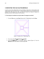
Do cuts
With the option Do cuts the user can make cuts through entities.
Makes parallel sections,
defining an axis in the normal
direction to the cuts, and the
number of divisions desired
along this axis
Divides volume sets in
two parts, cutting through
two points and relative to
the plane perpendicular to
the screen, or by three
Creates a set with the user
selection
Divides surface sets in two
parts, cutting through two
points and relative to the
plane perpendicular to the
screen, or by three points
Makes section through a
plane. This can be defined
by two points and relative to
the plane perpendicular to
the screen, or by three points
Makes a spherical cut
With this options cuts can be
converted to surface sets so
they can be saved, or cut
again
The user specifies a plane
which is used to get the lines
at one side of this plane
GID USER MANUAL
15
View results
This option permits the user to choose the viewing type in which the results of the postprocess
calculation will be presented.
Results are not viewed
Graphs are not viewed
Selects for which step of
analysis results will be
viewed
Same as contour fill, but with
defined ranges.
Chooses which result to view
in colored iso areas
Chooses which result to view
in smoothed colored iso
areas
Chooses which result to view
in colored lines
Shows outline of a particle by
vector field as lines tangent
to the result vectors
Shows location and value of
a selected maximum and
minimum numerical result
Selects which vector
result to view
Creates iso areas of the
results showing with colored
strips the place where each
subdivision finished
Graphs
Draws a scalar result
following the element Shows mesh deformation
according to a
normal
displacement field
Graph-style lines will be
drawn over the line elements
(only active when line
elements are used in the
mesh)
16
PRESENTATION OF GID
Options
Options permit the user to make choices related to the presentation of results: for example,
color changes, number of result subdivisions, etc.
Selects box which
shows the value
scale of the results.
Changes color
assigned to the
volume, surface and
cut sets.
Changes the name
assigned to the volume,
surface and cut sets.
How volumes,
surfaces and cuts
should be drawn
Allows user to
select the number
of colors in the
chromatic scale,
size of the
intervals, color
scale, etc.
Selects viewing
options of iso areas
Stream lines
options: kind of
label, color, and
delete option.
Defines options for
viewing graphics
User can choose
how to view the
vectors which
define the results
Elevations are lines that
connect the nodes and the
gauss points of the line
element and the graph style
line that represents the result
Defines options
surfaces
for
result
GID USER MANUAL
Postprocess windows
17
18
PRESENTATION OF GID
2. TOOLBARS
Option UtilitiesÆGraphicalÆToolbars opens a window where it’s possible to configure the
toolbars position or switch them on and off.
Geometry and View operations
(preprocess)
Zoom in: enlarges image area which
user indicates by drawing a mouse
window
Zoom out: reduces image area
which user indicates by drawing a
mouse window
Zoom frame: places image in center
of screen
Redraw: redraws image
Rotate trackball: rotates the image
Pan two points: displaces image
from one point to another, both
chosen by the user
Create NURBS line: creates a line of
type NURBS
Create polyline: creates polyline
apart from other lines
Create NURBS surface: creates a
NURBS surface defined by border
lines
Create volume: creates a volume
Create object: rectangle, circle,
polygon, sphere, cylinder, cone,
prism, thorus.
Delete: deletes entities
Create line: creates straight line
Create arc: creates an arc
List entities: permits listing of project
entities
Toggle geometry/mesh view
GID USER MANUAL
19
Standard toolbar
Creates a
new
project
Reads a
previously
created GiD
project
Prints the
current
project
Saves to
disc all
information
related to
the project
Changes the
configuration for Opens the copy
window
postprocess
phase
opens the
preferences
window
Opens the
layers window
Saves the
drawing
image shown
on the
screen, in
one of the
following
formats:
Opens the help
window
GiD info
button
Quits GiD
20
PRESENTATION OF GID
Geometry and View operations
(postprocess)
Zoom in: enlarges image area which
user indicates by drawing a mouse
window
Switch volume
sets on or off
Zoom out: reduces image area
which user indicates by drawing a
mouse window
Switch surface
sets on or off
Zoom frame: places image in center
of screen
Switch cut sets
on or off
redraw: redraws image
Do cuts: 2 points, 3
points, succession
axis
Rotate trackball: rotates the image
Pan two points: displaces image
from one point to another, both
chosen by the user
Set maximum value
(Contour fill)
Change light vector direction: with
this option the user can change the
vector of the light direction
interactively
Set minimum value
(Contour fill)
Reset contour limit
values (Contour fill)
Display style:
how volumes,
surfaces and cuts
should be drawn
Culling style:
none, front faces,
back faces or front
and back Faces.
List entities: permits
listing of project entities
GID USER MANUAL
21
3. MOUSE MENU
The Mouse Menu is the auxiliary menu which appears by clicking on the right mouse button
while the cursor is over the GiD screen.
The Mouse Menu permits the user to quickly access various image placement and viewing
commands, to facilitate easy management and definition of the project.
Furthermore, the Mouse Menu contains the Contextual menu, which permits the user to
access to all options available in previously performed commands. The option Contextual is
only available after the user has performed a command from the Top Menu.
User can access options
available in each distinct
command, once they have
been executed
Offers various zoom options
for viewing of piece
Offers various
rotation options:
Permits translations of the
image, from one point to
another (two points), or
dynamically (dynamic)
Redraws geometry of the
project
Offers various illumination
options for the image
Show numbering of the
entities for preprocess as
well for postprocess
Copies the drawing
image shown on the
screen to the clipboard
closes GiD
Activates or de-activates the
layers which form the project
and changes entities from
one layer to another layer.
22
PRESENTATION OF GID
4. COMMAND LINE
The Command Line option allows the user to directly enter all executable GiD commands,
without accessing the commands through drop-down menus.
These commands should be written following the order which GiD would use to define them,
according to the Right buttons menus.
A side comment in reference to the Command Line: GiD does not distinguish between the use
of capital and small letters. In addition, in cases where ambiguities do not exist, commands
need not be written in entire words, but can be written with the primary characters of each word.
GID USER MANUAL
23
INITIATION TO GID
With this example, the user is introduced to the basic tools for the creation of geometric entities
and mesh generation.
24
INITIATION TO GID
FIRST STEPS
Before presenting all the possibilities that GiD offers, we will present a simple example that will
introduce and familiarize the user with the GiD program.
The example will develop a finite element problem in one of its principal phases, the preprocess,
and will include the consequent data and parameter description of the problem. This example
introduces creation, manipulation and meshing of the geometrical entities used in GiD.
First, we will create a line and the mesh corresponding to the line. Next, we will save the project
and it will be described in the GiD data base form. Starting from this line, we will create a square
surface, which will be meshed to obtain a surface mesh. Finally, we will use this surface to
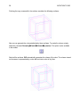
create a cubic volume, from which a volume mesh can then be generated.
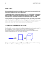
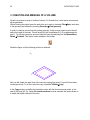
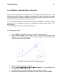
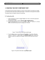
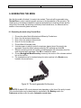
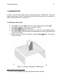
1. CREATION AND MESHING OF A LINE
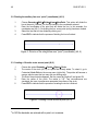
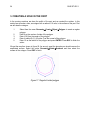
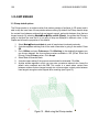
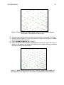
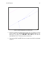
We will begin the example creating a line by defining its origin and end points, points 1 and 2 in
the following figure, whose coordinates are (0,0,0) and (10,0,0) respectively.
It is important to note that in creating and working with geometric entities, GiD follows the
following hierarchical order: point, line, surface, and volume.
1
2
1
2
1
2
To begin working with the program, open GiD, and a new GiD project is created automatically.
From this new database, we will first generate points 1 and 2.
GID USER MANUAL
25
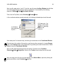
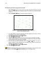
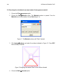
Next, we will create points 1 and 2. To do this, we will use an Auxiliary Window that will allow
us to simply describe the points by entering coordinates. It is accessed by the following
sequence: UtilitiesÆToolsÆCoordinates Window
Then, from the Top Menu, select GeometryÆCreateÆPoint
In the coordinate window opened previously, the following indicated steps should be used:
(1) Introduce
the coordinates
of point 1
(2) Create point 1 by
clicking on the button
Apply or by pressing
Enter on the
keyboard
And create point 2 in the same way, introducing its coordinates in the Coordinates Window.
The last step in the creation of the points, as well as any other command, is to press Escape,
either via the Escape button on the keyboard or by pressing the central mouse button. Select
Close to close the Coordinates Window.
Now, we will create the line that joins the two points. Choose from the Top Menu:
GeometryÆCreateÆStraight line. Option in the Toolbar shown below can also be used.
Next, the origin point of the line must be defined. In the Mouse Menu, opened by clicking the
right mouse button, select ContextualÆJoin C-a.
26
INITIATION TO GID
NOTE: With option Join, a point already created can be selected on the screen. The
command No Join is used to create a new point that has the coordinates of the point that is
selected on the screen. We can see that the cursor changes form for the Join and No Join
commands.
Cursor during use of Join command
Cursor during use of No Join command
Now, choose on the screen the first point, and then the second, which define the line. Finally,
press Escape to indicate that the creation of the line is completed.
NOTE: It is important to note that the Contextual submenu in the Mouse Menu will always
offer the options of the command that is currently being used. In this case, the corresponding
submenu for line creation, has the following options:
GID USER MANUAL
27
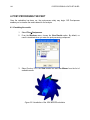
Once the geometry has been created, we can proceed to the line meshing. In this example, this
operation will be presented in the simplest and most automatic way that GiD permits. To do this,
from the Top Menu select: MeshÆGenerate mesh.
And an Auxiliary Window appears, in which the size of the elements should be defined by the
user.
NOTE: The size of an element with two nodes is the length of the element. For, surfaces
or volumes, the size is the mean length of the edge of the element.
In this example, the size of the element is defined in concordance with the length of the line,
chosen for this case as size 1.
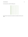
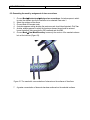
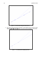
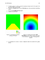
Automatically GiD generates a mesh for the line. The finite element mesh is presented on the
screen in a green color.
The mesh is formed by ten linear elements of two nodes. To see the numbering of the nodes
and mesh elements, select from the Mouse Menu: LabelÆAll, and the numbering for the 10
elements and 11 nodes will be shown, as below.
28
INITIATION TO GID
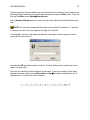
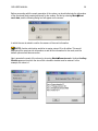
Once the mesh has been generated, the project should be saved. To save the example select
from the Top Menu: FilesÆSave.
The program automatically saves the file if it already has a name. If it is the first time the file has
been saved, the user is asked to assign a name. For this, an Auxiliary Window will appear
which permits the user to browse the computer disk drive and select the location in which to
save the file. Once the desired directory has been selected, the name for the actual project can
be entered in the space titled File Name.
NOTE: Next, the manner in which GiD saves the information of a project will be explained.
GiD creates a directory with a name chosen by the user, and whose file extension is .gid. GiD
creates a set of files in this directory where all the information generated in the present example
is saved. All the files have the same name of the directory to which they belong, but with
different extensions. These files should have the name that GiD designates and should not be
changed manually.
Each time the user selects option save the database will be rewritten with the new information
or changes made to the project, always maintaining the same name.
To exit GiD, simply choose FilesÆQuit.
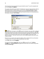
To access the example, ejemplo.gid, simply open GiD and select from the Top Menu:
FilesÆOpen. An Auxiliary Window will appear which allows the user to access and open the
directory iniciación.gid.
GID USER MANUAL
29
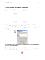
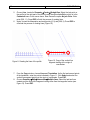
2. CREATION AND MESHING OF A SURFACE
We will now continue with the creation and meshing of a surface.
First, we will create a second line between points 1 and 3.
3 (0,10,0)
1 (0,0,0)
2 (10,0,0)
We will now generate the second line. We will now use again the Coordinates Window to enter
the points. (UtilitiesÆToolsÆCoordinates Window)
Select the line creation tool in the toolbar. Enter point (0,10,0) in the Coordinates Window and
click Apply.
With option Join (Contextual mouse menu) click over point 1. A line should be created between
(0,10,0) and (0,0,0). Press Escape.
With this, a right angle of the square has been defined. If the user wants to view everything that
has been created to this point, the image can be centered on the screen by choosing in the
Mouse Menu: ZoomÆFrame. This option is also available in the toolbar.
30
INITIATION TO GID
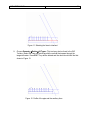
Finish the square by creating point (10,10,0) and the lines that join this point with points 2 and 3.
3 (0,10,0)
1 (0,0,0)
2 (10,0,0)
Now, we will create the surface that these four lines define. To do this, access the create
surface command by choosing: GeometryÆCreateÆNURBS surfaceÆBy contour. This
option is also available in the toolbar:
GiD then asks the user to define the 4 lines that describe the contour of the surface. Select the
lines using the cursor on the screen, either by choosing them one by one or selecting them all
with a window. Next, press Escape.
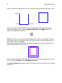
As can be seen below, the new surface is created and appears as a smaller, magenta-colored
square drawn inside the original four lines.
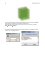
Once the surface has been created, the mesh can be created in the same way as was done for
the line. From the Top Menu select: MeshÆGenerate mesh.
An Auxiliary Window appears which asks for the maximum size of the element, in this example
defined as 1.
GID USER MANUAL
31
We can see that the lines containing elements of two nodes have not been meshed. Rather the
mesh generated over the surface consists of planes of three-nodded, triangular elements.
NOTE: GiD meshes by default the entity of highest order with which it is working.
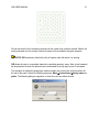
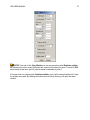
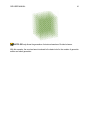
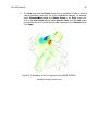
GiD allows the user to concentrate elements in specified geometry zones. Next, a brief example
will be presented in which the elements are concentrated in the top right corner of the square.
This operation is realized by assigning a smaller element size to the point in this zone than for
the rest of the mesh. Select the following sequence: MeshÆ UnstructuredÆAssign sizes on
points. The following dialog box appears, in which the user can define the size:
32
INITIATION TO GID
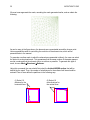
We must now regenerate the mesh, canceling the mesh generated earlier, and we obtain the
following:
As can be seen in the figure above, the elements are concentrated around the chosen point.
Various possibilities exist for controlling the evolution of the element size, which will be
presented later in the manual.
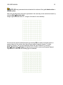
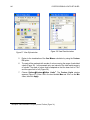
To generate a surface mesh in which the elements are presented uniformly, the user can select
the option for a structured mesh. This guarantees that the same number of elements appears
around a node and that the element size is as uniform as possible. To generate this type of
mesh, choose: MeshÆStructuredÆSurfaces.
Using this command, the user should first select the 4-sided NURBS surface that will be
defined by the mesh. Then, the number of subdivisions for the surface limit lines should be
entered. Pairs of lines define the partitions in the following way:
(1) Select 10
divisions for the
horizontal lines
(2) Select 10
more divisions for
the vertical lines
GID USER MANUAL
33
NOTE: GiD only generates structured meshes for surfaces of the type 4-sided surface or
NURBS surface.
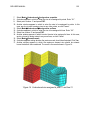
When this has been done, the mesh is generated in the same way as the unstructured mesh, by
choosing MeshÆGenerate mesh.
Assign a general element size of 1, though in this case it is not necessary.
We can see here that the default element type used by GiD to create a structured mesh is a
square element of four nodes rather than a three-nodded, triangular element. To obtain
triangular elements, the user can specifically define this type of element, by choosing
MeshÆElement typeÆTriangle, and selecting the surface to mesh as a triangular element.
Regenerate the mesh, and the following figure is obtained:
34
INITIATION TO GID
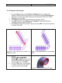
GiD also allows the user to concentrate elements in structured meshes. This can be done by
selecting MeshÆStructuredÆLinesÆConcentrate elements
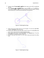
First, we must select the lines that need to be assigned an element concentration weight. The
value of this weight can be either positive or negative, depending on whether the user wants to
concentrate elements at the beginning or end of the lines. Next, a vector appears which defines
the start and end of the line and which helps the user assign the weight correctly.
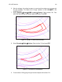
Select the top line and assign a weight of 0.5 to the end of the line:
Select the bottom line and assign a weight of 0.5 to the beginning of the line:
GID USER MANUAL
From these operations, we obtain the following mesh:
We can see that in the figure above, the elements are concentrated in the left zone of the
square.
35
36
INITIATION TO GID
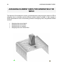
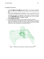
3. CREATION AND MESHING OF A VOLUME
We will now present a study of entities of volume. To illustrate this, a cube and a volume mesh
will be generated.
Without leaving the project, save the work done up to now by choosing FilesÆSave, and return
to the geometry last created by choosing GeometryÆView geometry.
In order to create a volume from the existing geometry, firstly we must create a point that will
define the height of the cube. This will be point 5 with coordinates (0,0,10), superimposed on
point 1. To view the new point, we must rotate the figure by selecting from the Mouse Menu,
RotateÆTrackball. This option is also available in the toolbar:
Rotate the figure until the following position is achieved:
5
1
Next, we will create the upper face of the cube by copying from point 1 to point 5 the surface
created previously. To do this, select the copy command, UtilitiesÆCopy.
In the Copy window, we define the translation vector with the first and second points, in this
case (0,0,0) and (0,0,10). Option Do extrude surfaces must be selected; this option allows us
to create the lateral surfaces of the cube.
GID USER MANUAL
37
NOTE: If we look at the Copy Window, we can see an option called Duplicate entities.
By activating this option, when the entities are copied (in this case from point 1 to point 5) GiD
would create a new point (point 6) with the same coordinates as point 5.
If the user does not choose option Duplicate entities, point 6 will be merged with point 5 when
the entities are copied. By labeling the entities we could verify that only one point has been
created.
38
INITIATION TO GID
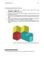
Finishing the copy command for the surface, we obtain the following surfaces:
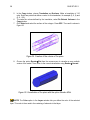
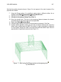
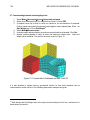
Now, we can generate the volume delimited by these surfaces. To create the volume, simply
select the command GeometryÆCreateÆVolumeÆBy contour. This option is also available
in the toolbar:
Select all the surfaces. GiD automatically generates the volume of the cube. The volume viewed
on the screen is represented by a cube with an interior color of sky blue.
GID USER MANUAL
39
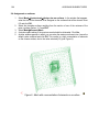
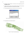
Before proceeding with the mesh generation of the volume, we should eliminate the information
of the structured mesh created previously for the surface. Do this by selecting MeshÆReset
mesh data, and the following dialog box will appear on the screen:
In which the user is asked to confirm the erasure of the mesh information.
NOTE: Another valid option would be to assign a size of 0 to all entities. This would
eliminate all the previous size information as well as the information for the mesh, and the
default options would become active.
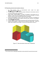
Next, generate the mesh of the volume by choosing MeshÆGenerate mesh. Another Auxiliary
Window appears into which the size of the volumetric element must be entered. In this
example, the value is 1.
40
INITIATION TO GID
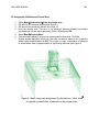
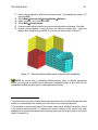
The mesh generated above is composed of tetrahedral elements of four nodes, but GiD also
permits the use of hexahedral, eight-nodded structured elements.
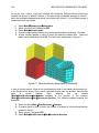
We will generate a structured mesh of the volume of the cube. This is done by selecting
MeshÆStructuredÆVolumes.
Now select the volume to mesh and enter the number of partitions in its edges which will be
created. Then, create again the mesh.
GID USER MANUAL
41
NOTE: GiD only allows the generation of structured meshes of 6-sided volumes.
With this example, the user has been introduced to the basic tools for the creation of geometric
entities and mesh generation.
42
CASE STUDY 1
CASE STUDY 1
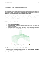
IMPLEMENTING A MECHANICAL PART
The objective of this case study is implementing a mechanical part in order to study it through
meshing analysis. The development of the model consists of the following steps:
•
•
•
Creating a profile of the part
Generating a volume defined by the profile
Generating the mesh for the part
At the end of this case study, you should be able to handle the 2D tools available in GiD as well
as the options for generating meshes and visualizing the prototype.
GID USER MANUAL
43
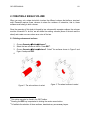
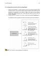
1. WORKING BY LAYERS
1.1. Defining the layers
A geometric representation is composed of four types of entities, namely points, lines, surfaces,
and volumes.
A layer is a grouping of entities. Defining layers in computer-aided design allows us to work
collectively with all the entities in one layer.
The creation of a profile of the mechanical part in our case study will be carried out with the help
of auxiliary lines. Two layers will be defined in order to prevent these lines from appearing in the
final drawing. The lines that define the profile will be assigned to one of the layers, called the
“profile” layer, while the auxiliary lines will be assigned to the other layer, called the “aux” layer.
When the design of the part has been completed, the entities in the “aux” layer will be erased.
44
CASE STUDY 1
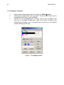
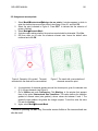
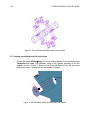
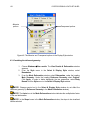
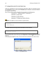
1.2. Creating two new layers
1.
2.
3.
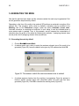
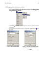
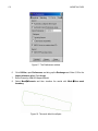
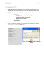
Open the layer management window. This is found in UtilitiesÆLayers.
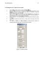
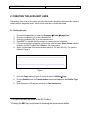
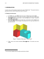
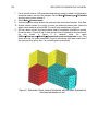
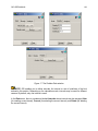
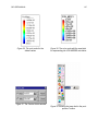
Create two new layers called “aux” and “profile.” Enter the name of each layer in
the Layers window (Figure 1) and click New.
Choose “aux” as the activated layer. To do this, click on “aux” to highlight it and
then click on the Layer To Use button. (Next to this button the name of the
activated layer will appear, “aux” in the present case.) From now on, all the entities
created will belong to this layer.
Figure 1. The Layers window
GID USER MANUAL
45
2. CREATING A PROFILE
In our case, the profile consists of various teeth. Begin by drawing one of these teeth, which will
be copied later to obtain the entire profile.
2.1. Creating a size-55 auxiliary line
1.
2.
3.
4.
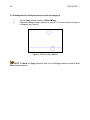
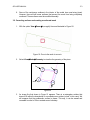
Choose the Line option, by going to GeometryÆCreateÆStraight line or by
going to the GiD Toolbox1.
2
Enter the coordinates of the beginning and end points of the auxiliary line . For our
example, the coordinates are (0, 0) and (55, 0), respectively. Besides creating a
straight line, this operation implies creating the end points of the line.
3
Press ESC to indicate that the process of creating the line is finished.
If the entire line does not appear on the screen, use the Zoom Frame option,
which is located in the GiD Toolbox and in Zoom in the mouse menu.
Figure 2. Creating a straight line
NOTE: The Undo option, located in UtilitiesÆUndo, enables you to undo the most recent
operations. When this option is selected, a window appears in which all the operations to be
undone can be selected.
1
The GiD Toolbox is a window containing the icons for the most frequently executed
operations. For information on a particular tool, click on the corresponding icon with the right
mouse button.
2
The coordinates of a point may be entered on the command line either with a space or a
comma between them. If the Z coordinate is not entered, it is considered 0 by default. After
entering the numbers, press Return. Another option for entering a point is using the
Coordinates Window, found in UtilitiesÆToolsÆCoordinates Window.
3
Pressing the ESC key is equivalent to pressing the center mouse button.
46
CASE STUDY 1
2.2. Dividing the auxiliary line near “point” (coordinates) (40, 0)
1.
2.
3.
4.
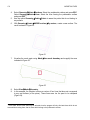
Choose GeometryÆEditÆDivideÆLinesÆNearPoint. This option will divide the
line at the point (“element”) on the line closest to the coordinates entered.
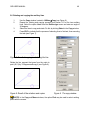
Enter the coordinates of the point that will divide the line. In this example, the
coordinates are (40, 0). On dividing the line, a new point (entity) has been created.
Select the line that is to be divided by clicking on it.
Press ESC to indicate that the process of dividing the line is finished.
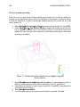
Figure 3. Division of the straight line near “point” (coordinates) (40, 0)
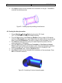
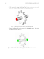
2.3. Creating a 3.8-radius circle around point (40, 0)
1.
2.
3.
4.
5.
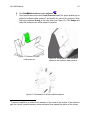
Choose the option GeometryÆCreateÆObjectÆCircle.
The center of the circle (40, 0) is a point that already exists. To select it, go to
ContextualÆJoin Ctrl-a in the mouse menu (right-click). The pointer will become a
square, which means that you may click an existing point.
The Enter Normal window appears. Set the normal as Positive Z and press OK.
4
Enter the radius of the circle. The radius is 3.8 . Two circumferences are
visualized; the inner circumference represents the surface of the circle.
Press ESC to indicate that the process of creating the circle is finished.
Figure 4. Creating a circle around a point (40, 0)
4
In GiD the decimals are entered with a point, not a comma.
GID USER MANUAL
47
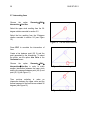
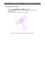
2.4. Rotating the circle -3 degrees around a point
1.
2.
3.
4.
5.
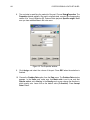
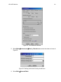
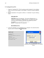
6.
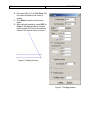
Use the Move window, which is located in UtilitiesÆMove.
Within the Move menu and from among the Transformation possibilities, select
Rotation. The type of entity to receive the rotation is a surface, so from the
Entities Type menu, choose Surfaces.
Enter -3 in the Angle box and check the Two dimensions box. (Provided we
define positive rotation in the mathematical sense, which is counter-clockwise, -3
degrees equates to a clockwise rotation of 3 degrees.)
Enter the point (0, 0, 0) under First Point. This is the point that defines the center
of rotation.
Click Select to select the surface that is to rotate, which in this case is that of the
circle.
Press ESC (or Finish in the Move window) to indicate that the selection of
surfaces to rotate has been made, thus executing the rotation.
Figure 5. The Move window
48
CASE STUDY 1
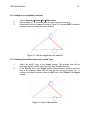
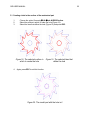
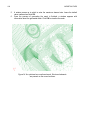
2.5. Rotating the circle 36 degrees around a point and copying it.
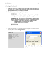
1.
2.
Use the Copy window, located in UtilitiesÆCopy.
Repeat the rotation process explained in section 2.4, but this time with an angle of
36 degrees (see Figure 6).
Figure 6. Result of the rotations
NOTE: The Move and Copy operations differ only in that Copy creates new entities while
Move displaces entities.
GID USER MANUAL
49
2.6. Rotating and copying the auxiliary lines
1.
2.
3.
4.
Use the Copy window, located in UtilitiesÆCopy (see Figure 9).
Repeat the rotating and copying process from section 2.5 for the two auxiliary
lines. Select the option Lines from the Entities type menu and enter an angle of
36 degrees.
Select the lines to copy and rotate. Do this by clicking Select in the Copy window.
Press ESC to indicate that the process of selecting lines is finished, thus executing
the task (see Figure 7).
Figure 7. Result of copying and rotating the line.
Rotate the line segment that goes from the origin to
point (40, 0) by 33 degrees and copy it (see Figure 8).
Figure 8. Result of the rotations and copies
Figure 9. The copy window
NOTE: In the Copy and Move windows, the option Pick may be used to select existing
points with the mouse.
50
CASE STUDY 1
2.7. Intersecting lines
Choose
the
option
IntersectionÆLine-line.
GeometryÆEditÆ
Select the upper circle resulting from the 36degree rotation executed in section 2.5.
Select the line resulting from the 33-degree
rotation executed in section 2.6 (see Figure
10).
Figure 10. The two lines selected
Press ESC to conclude the intersection of
lines.
Create a line between point (55, 0) and the
point generated by the intersection. To select
the points, use the option Join Ctrl-a in the
Contextual menu.
Choose
the
option
GeometryÆEditÆ
IntersectionÆLine-line in order to make
another intersection between the lower circle
and the line segment between point (40, 0) and
point (55, 0) (see Figure 11).
Figure 11. Intersecting lines
Then continue selecting to make an
intersection between the upper circle and the
farthest segment of the line that was rotated 36
degrees (see Figure 12).
Figure 12. Intersecting lines
GID USER MANUAL
51
2.8. Creating an arc tangential to two lines
1.
2.
3.
Choose GeometryÆCreateÆArcÆFillet curves.
Enter a radius of 1.35 in the command line (see footnote 2 on page 4).
Now select the two line segments shown in Figure 13. Then press ESC to indicate
that the process of creating the arcs is finished.
Figure 13. The line segments to be selected
2.9. Translating the definitive lines to the “profile” layer
1.
2.
Select the “profile” layer in the Layers window. The auxiliary lines will be
eliminated and the “profile” layer will contain only the definitive lines.
In the Sent To menu of the Layers window, choose Lines in order to select the
lines to be translated. Select only the lines that form the profile (Figure 14). To
conclude the selection process, press the ESC key or click Finish in the Layers
window.
Figure 14. Lines to be selected
52
CASE STUDY 1
2.10. Deleting the “aux” layer
1.
2.
3.
4.
5.
6.
Click Off the profile layer.
Choose GeometryÆDeleteÆAll Types (or use the GiD Toolbox).
Select all the lines and surfaces that appear on the screen. (The click-and-drag
technique may be used to make the selection.)
Press ESC to conclude the selection of elements to delete.
Select the “aux” layer in the Layers window and click Delete.
Select the “profile” layer.
NOTE: When a layer is clicked Off, GiD reminds you of this. From this moment on,
whatever is drawn does not appear on the screen since it is in the hidden layer.
NOTE: To cancel the deletion of elements after they have been selected, open the mouse
menu, go to Contextual and choose Clear Selection.
NOTE: Elements forming part of higher level entities may not be deleted. For example, a
point that defines a line may not be deleted.
NOTE: A layer containing information may not be deleted. First the contents must be
deleted.
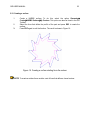
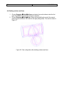
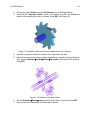
2.11. Rotating and obtaining the final profile
1.
2.
3.
4.
5.
Make sure that the activated layer is the “profile” layer. (Use the option Layer To
use.)
In the Copy window, select the line rotation (Rotation, Lines).
Enter an angle of 36 degrees. Make sure that the center is point (0, 0, 0) and that
you are working in two dimensions.
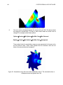
In the Multiple Copies box enter 9. This way, 9 copies will be made, thus
obtaining the 10 teeth that form the profile of the model (9 copies and the original).
Click Select and select the profile. Press the ESC key or click Finish in the Copy
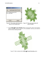
window in order to conclude the operation. The result is shown in Figure 15.
Figure 15. The part resulting
from this process
GID USER MANUAL
53
2.12. Creating a surface
1.
2.
3.
Create a NURBS surface. To do this, select the option GeometryÆ
CreateÆNURBS SurfaceÆBy Contour. This option can also be found in the GiD
Toolbox.
Select the lines that define the profile of the part and press ESC to create the
surface.
Press ESC again to exit the function. The result is shown in Figure 16.
Figure 16. Creating a surface starting from the contour
NOTE: To create a surface there must be a set of lines that define a closed contour.
54
CASE STUDY 1
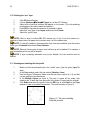
3. CREATING A HOLE IN THE PART
In the previous sections we drew the profile of the part and we created the surface. In this
section we will make a hole, an octagon with a radius of 10 units, in the surface of the part. First
we will draw the octagon.
1.
2.
3.
4.
5.
Select from the menu GeometryÆCreateÆObjectÆPolygon to create a regular
polygon.
Enter 8 as the number of sides of the polygon.
Enter (0,0,0) as the center of the polygon.
Enter or select (0,0,1) (Positive Z) as the normal of the polygon.
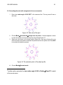
Enter 10 as the radius of the polygon and press ENTER. Press ESC to finish the
action.
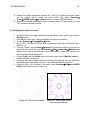
We get the result as shown in figure 20. As we only need the boundary we should remove the
associated surface. Select the option GeometryÆDeleteÆSurfaces and then select the
surface of the octagon. Press ESC to finish.
Figure 17. Regular 8-sided polygon
GID USER MANUAL
55
3.1. Creating a hole in the surface of the mechanical part
1.
2.
3.
Choose the option GeometryÆEditÆHole NURBS Surface.
Select the surface in which to make the hole (Figure 18).
Select the lines that define the hole (Figure 19) and press ESC.
Figure 18. The selected surface in
which to create the hole
4.
Figure 19. The selected lines that
define the hole
Again, press ESC to exit this function.
Figure 20. The model part with the hole in it
56
CASE STUDY 1
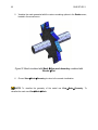
4. CREATING VOLUMES FROM SURFACES
The mechanical part to be constructed is composed of two volumes: the volume of the wheel
(defined by the profile), and the volume of the axle, which is a prism with an octagonal base that
fits into the hole in the wheel. Creating this prism will be the first step of this stage. It will be
created in a new layer that we will name “prism”.
4.1. Creating the “prism” layer and translating the octagon to this layer
1.
2.
3.
4.
In the Layers window, type the name of the new layer and click New.
Select the “prism” layer and click Layer To use to choose it as the activated layer.
Choose Lines in the Sent To menu in the Layers window. Select the lines that define
the octagon. Press ESC to conclude the selection.
Select the “profile” layer and click Off to deactivate it.
Figure 21. The lines that form the octagon
GID USER MANUAL
57
4.2. Creating the volume of the prism
1.
2.
First copy the octagon a distance of -50 units relative to the surface of the wheel, which
is where the base of the prism will be located. In the Copy window, choose
Translation and Lines. Since we want to translate 50 units, enter two points that
define the vector of this translation, for example (0, 0, 0) and (0, 0, 50). (Make sure that
the Multiple Copies value is 1, since last time the window was used its value was 9).
Choose Select and select the lines of the octagon. Press ESC to conclude the
selection.
Figure 22. Selection of the lines that form the octagon
3.
Since the Z axis is parallel to the user’s line of vision, the perspective must be changed
to visualize the result. To do this, use the Rotate Trackball tool, which is located in the
GiD Toolbox and in the mouse menu.
Figure 23. Copying the octagon and changing the perspective
4.
Choose GeometryÆCreateÆNURBS surfaceÆBy contour. Select the lines that
form the displaced octagon and press ESC to conclude the selection. Again, press
ESC to exit the function of creating the surfaces.
Figure 24. The surface created on the translated octagon
58
CASE STUDY 1
5.
6.
7.
In the Copy window, choose Translation and Surfaces. Make a translation of 110
units. Enter two points that define a vector for this translation, for example (0, 0, 0) and
(0, 0, -110).
To create the volume defined by the translation, select Do Extrude Volumes in the
Copy window.
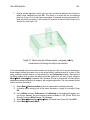
Click Select and select the surface of the octagon. Press ESC. The result is shown in
Figure 25.
Figure 25. Creation of the volume of the prism
8.
Choose the option RenderÆFlat from the mouse menu to visualize a more realistic
version of the model. Then return to the normal visualization using RenderÆ Normal.
Figure 26. Visualization of the prism with the option RenderÆFlat.
NOTE: The Color option in the Layers window lets you define the color of the selected
layer. This color is then used in the rendering of elements in that layer.
GID USER MANUAL
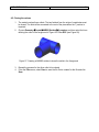
59
4.3. Creating the volume of the wheel
1.
2.
3.
4.
5.
6.
7.
Visualize the “profile” layer and activate it. The volume of the wheel will be created in
this layer. Deactivate the “prism” layer in order to make the selection of the entities
easier.
In the Copy window, choose Translation and Surfaces. A translation of 10 units will
be made. To do this, enter two points that define a vector for this translation, for
example (0, 0, 0) and (0, 0, -10).
Choose the option Do Extrude Volumes from the Copy window. The volume that is
defined by the translation will be created.
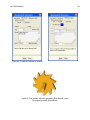
Make sure that the Maintain Layers option is not checked.
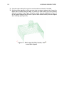
Click Select and select the surface of the wheel. Press ESC.
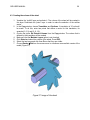
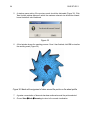
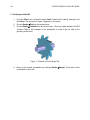
Select the two layers and click them On so that they are visible.
Choose RenderÆFlat from the mouse menu to visualize a more realistic version of the
model (Figure 27).
Figure 27. Image of the wheel
60
CASE STUDY 1
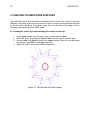
5. GENERATING THE MESH
Now that the part has been drawn and the volumes created, the mesh may be generated. First
we will generate a simple mesh by default.
Depending on the form of the entity to be meshed, GiD performs an automatic correction of the
element size. This correction option, which by default is activated, may be modified in the
Meshing card of the Preferences window, under the option Automatic correct sizes.
Automatic correction is sometimes not sufficient. In such cases, it must be indicated where a
more precise mesh is needed. Thus, in this example, we will increase the concentration of
elements along the profile of the wheel by following two methods: 1) assigning element sizes
around points, and 2) assigning element sizes around lines.
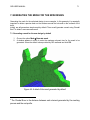
5.1. Generating the mesh by default
1.
2.
Choose MeshÆGenerate Mesh.
A window comes up in which to enter the maximum element size of the mesh to be
generated (Figure 28). Leave the default value given by GiD unaltered and click OK.
Figure 28. The window in which the maximum element size is entered
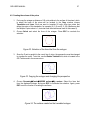
3.
A window appears showing how the meshing is progressing. Once the process is
finished, another window opens with information about the mesh that has been
generated (Figure 29). Click OK to visualize the resulting mesh (Figure 30).
GID USER MANUAL
Figure 29. The window with information
about the mesh generated
4.
61
Figure 30. The mesh generated with
default settings
Use the MeshÆView mesh boundary option to see only the contour of the volumes
meshed without the interiors (Figure 31). This visualization mode may be combined
with the various rendering methods.
Figure 31. Mesh visualized with the MeshÆView mesh boundary option
62
CASE STUDY 1
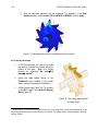
5.
Visualize the mesh generated with the various rendering options in the Render menu,
located in the mouse menu.
Figure 32. Mesh visualized with MeshÆView mesh boundary combined with
RenderÆFlat.
6.
Choose ViewÆModeÆGeometry to return to the normal visualization.
NOTE: To visualize the geometry of the model use ViewÆModeÆGeometry. To
visualize the mesh use ViewÆModeÆMesh.
GID USER MANUAL
63
5.2. Generating the mesh with assignment of size around points
1.
5
Enter view rotate angle -90 90 ESC in the command line. This way we will have a
side view.
Figure 33. Side view of the part.
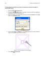
2.
3.
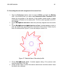
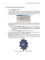
Choose MeshÆUnstructuredÆAssign sizes on points. A window appears in which
to enter the element size around the point to be selected. Enter 0.7.
Select only the points on the wheel profile (Figure 34). One way of doing this is to
select the entire part and then deselect the points that form the prism hole. Press ESC
to conclude the selection process.
Figure 34. The selected points of the wheel profile
4.
5
Choose MeshÆGenerate mesh.
Another option equivalent to view rotate angle -90 90 is RotateÆPlane XY, located
in the mouse menu.
64
CASE STUDY 1
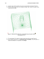
5.
A window opens asking if the previous mesh should be eliminated (Figure 35). Click
Yes. Another window appears in which the maximum element size should be entered.
Leave the default value unaltered.
Figure 35
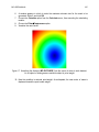
6.
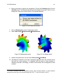
A third window shows the meshing process. Once it has finished, click OK to visualize
the resulting mesh (Figure 36).
Figure 36. Mesh with assignment of sizes around the points on the wheel profile
7.
8.
A greater concentration of elements has been achieved around the points selected.
Choose ViewÆModeÆGeometry to return to the normal visualization.
GID USER MANUAL
65
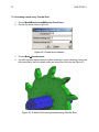
5.3. Generating the mesh with assignment of size around lines
1.
2.
3.
Open the Preferences window, which is found in Utilities, and select the Meshing
card. In this window there is an option called Unstructured Size Transitions which
defines the size gradient of the elements. A high gradient number means a greater
concentration of elements on the wheel profile. To do this, select a gradient size of 0.8.
Click Accept.
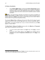
Choose MeshÆReset mesh data to delete the previously assigned sizes from section
5.2.
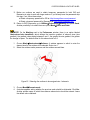
Choose MeshÆUnstructuredÆAssign sizes on lines. A window appears in which to
enter the element size around the lines to be selected. Enter size 0.7. Select only the
lines of the wheel profile (Figure 37) in the same way as in section 5.2.
Figure 37. Selected lines of the wheel profile
4.
5.
Choose MeshÆGenerate mesh. A window appears asking if the previous mesh
should be eliminated. Click Yes.
Another window opens in which the maximum element size should be entered. Leave
the default value unaltered.
66
CASE STUDY 1
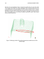
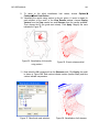
6.
A greater concentration of elements has been achieved around the selected lines. In
contrast to the case in section 5.2, this mesh is more accurate since lines define the
profile much better than points do (Figure 38).
Figure 38. Mesh with assignment of sizes around lines
GID USER MANUAL
67
6. OPTIMIZING THE DESIGN OF THE PART
The part we have designed can be optimized, thus achieving a more efficient product. Given
that the part will rotate clockwise, reshaping the upper part of the teeth could reduce the weight
of the part as well as increase its resistance. We could also modify the profile of the hole in
order to increase resistance in zones under axle pressure.
To carry out these optimizations, we will use new tools such as NURBS lines. The final steps in
this process will be generating a mesh and visualizing the changes made relative to the
previous design.
This example begins with a file named “optimizacion.gid”.
6.1. Modifying the profile
1.
2.
Choose Read from the Files menu and open the file “optimizacion.gid”.
The file contents appear on the screen. In order to work more comfortably, select
Zoom In, thus magnifying the image. This option is located both in the GiD Toolbox
and in the mouse menu under Zoom.
Figure 39. Contents of the file “optimizacion.gid”.
3.
4.
5.
6.
Make sure that the “aux” layer is activated.
Choose GeometryÆEditÆDivideÆLinesÆNum Divisions. This option divides a line
into a specified number of segments.
A window comes up in which to enter the number of partitions. Enter 8.
Select the line segment from the upper part of a tooth (Figure 39) and press ESC.
68
CASE STUDY 1
7.
8.
Using the option GeometryÆCreateÆPoint, and create a point with the coordinates
(40, 8.5).
Choose GeometryÆCreateÆNURBS line to create a NURBS curve. The NURBS line
to be created will pass through the two first points which have been created on dividing
the line at point (40, 8.5) and by the two last points of the divided line.
Figure 40. Optimizing the design
9.
Select the first point through which the curve will pass. To do this use Join Ctrl-a,
located in Contextual in the mouse menu.
10. One at a time, select the rest of the points except the last one. Use Join Ctrl-a each
time in order to ensure that the line passes through the point.
11. Before selecting the last point, choose Last Point in the Contextual menu. Then finish
the NURBS line. The result is shown in Figure 40.
12. Send the new profile (See Figure 41) to the “profile” layer and eliminate the auxiliary
lines.
Figure 41. Optimizing the design
GID USER MANUAL
69
13. Repeat the process explained in sections 2.11 and 2.12 to create the wheel surface:
use the rotation tool to create the entire profile and, using GeometryÆ
CreateÆNURBS SurfaceÆBy contour, select it to create a NURBS surface.
14. Repeat the processes explained in section 3 (except section 3.1) and sections 4.1 and
4.2 to create the prismatic volume.
6.2. Modifying the profile of the hole
1.
2.
3.
4.
5.
6.
7.
8.
Move the lines of the octagon placed in the profile surface to the “profile” layer (with the
Send To button).
Click Off the “prism” layer. Hiding it simplifies the space on the screen.
Choose GeometryÆCreateÆObjectÆCircle.
Enter (-10.5, 0) as the center point. Enter a normal to the XY plane (Positive Z) and a
radius of 1.5.
From the Toolbox, use the DeleteÆSurfaces tool to delete the surface of the circle so
that only the line is left. This way the GeometryÆEditÆ IntersectionÆMultiple Lines
option may be used to intersect the circle (circumference). Select only the circle and
the two straight lines that intersect it.
Choose Copy from the Utilities menu and make seven copies (Multiple copies=7),
rotating the circle -45 degrees.
Using the intersection options, delete the auxiliary lines leaving only the valid lines,
thus obtaining the new profile of the hole. The result is illustrated in Figure 42.
Create the hole in the surface of the wheel using GeometryÆEditÆHole NURBS
Surface (the result is shown in Figure 43).
Figure 42. The new hole profile
Figure 43. The surface of the
new optimized design
70
CASE STUDY 1
6.3. Creating the volume of the new design
Repeat the same process as in section 4.3:
1.
2.
3.
In the Copy window, choose Translation and Surfaces. Enter two points that define a
translation of 10 units, for example (0, 0, 10) and (0, 0, 0). (Make sure that the Multiple
Copies value is 1).
Choose Do Extrude Volume in the Copy window.
Click Select and select the surface of the wheel. Press ESC.
Figure 44. The volume of the optimized design
4.
Click On the “prism” layer.
GID USER MANUAL
71
7. GENERATING THE MESH FOR THE NEW DESIGN
Generating the mesh for the optimized design is more complex. In this geometry it is especially
important to obtain a precise mesh on the surfaces around the hole and on the surfaces of the
teeth.
Initially, we will generate a simple mesh by default. Then we will generate a mesh using Chordal
6
Error to obtain a more accurate result.
7.1. Generating a mesh for the new design by default
1.
2.
Choose the option MeshÆGenerate mesh.
A window appears in which to enter the maximum element size for the mesh to be
generated. Leave the default value provided by GiD unaltered and click OK.
Figure 45. A detail of the mesh generated by default
6
The Chordal Error is the distance between each element generated by the meshing
process and the real profile.
72
CASE STUDY 1
7.2. Generating a mesh using "Chordal Error"
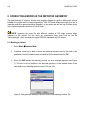
1.
2.
Choose MeshÆUnstructuredÆSizes by Chordal error.
Provide the values shown in figure 46.
Figure 46. Chordal error windows
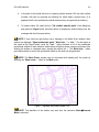
3.
4.
Choose MeshÆGenerate mesh.
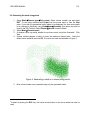
A greatly improved approximation has been achieved in zones containing curves and,
more specifically, along the wheel profile and the profile of the hole (see Figure 47).
Figure 47. A detail of the mesh generated using Chordal Error
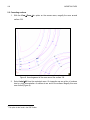
GID USER MANUAL
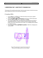
73
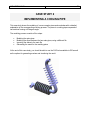
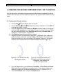
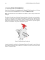
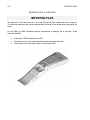
CASE STUDY 2
IMPLEMENTING A COOLING PIPE
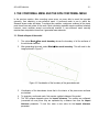
This case study shows the modeling of a more complex piece and concludes with a detailed
explanation of the corresponding meshing process. The piece is a cooling pipe composed of
two sections forming a 60-degree angle.
The modeling process consists of four steps:
•
•
•
•
Modeling the main pipes
Modeling the elbow between the two main pipes, using a different file
Importing the elbow to the main file
Generating the mesh for the resulting piece
At the end of this case study, you should be able to use the CAD tools available in GiD as well
as the options for generating meshes and visualizing the result.
74
CASE STUDY 2
1. WORKING BY LAYERS
Various auxiliary lines will be needed in order to draw the part. Since these auxiliary lines must
not appear in the final drawing, they will be in a different layer from the one used for the finished
model.
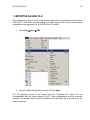
1.1. Creating two new layers
Open
the
layer
management
window,
which
is
found
in
the
UtilitiesÆLayers menu.
Create two new layers called “aux” and “ok”.
Enter the name for each layer in the Layers
window (Figure 1) and click New.
Choose “aux” as the activated layer. To do
this, click on "aux" to highlight it and then click
on the Layer To Use button. (The name of
the activated layer will appear next to the
button, "aux" in this case.) From now on, all
the entities created will belong to this layer.
Figure 1. The Layers window
GID USER MANUAL
75
2. CREATING THE AUXILIARY LINES
The auxiliary lines used in this project are those that make it possible to determine the center of
rotation and the tangential center, which will be used later to create the model.
2.1. Creating the axes
1.
2.
3.
4.
5.
6.
Choose the Line option, by selecting GeometryÆCreateÆStraight line1.
Enter the coordinate (0, 0) in the command line.
Enter the coordinate (200, 0) in the command line.
2
Press ESC to indicate that the process of creating the line is finished.
If the entire line does not appear on the screen, use the option Zoom Frame, which is
located in the GiD Toolbox and in Zoom in the mouse menu.
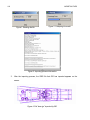
Again, choose Line. Draw a line between points (0, 25) and (200, 25). The result is
shown in Figure 2.
Figure 1
7.
8.
9.
Go to the Copy window (Figure 4), which is found in UtilitiesÆCopy.
Choose Rotation from the Transformation menu and Lines from the Entities Type
menu.
Enter an angle of -60 degrees and click on Two dimensions.
1
This option can also be found in the GiD Toolbox.
2
Pressing the ESC key is equivalent to pressing the center mouse button.
76
CASE STUDY 2
10. Enter point (200, 0, 0) in First Point. This
is the point that defines the center of
rotation.
11. Click Select to select the first line we
drawn.
12. After making the selection, press ESC (or
Finish in the Copy window) to indicate
that the selection of lines to be rotated is
finished. The result is shown in Figure 3.
Figure 2. Creating the axes
Figure 3. The Copy window
GID USER MANUAL
77
2.2. Creating the tangential center
1.
2.
3.
Choose the menu option GeometryÆCreateÆStraight line. On the mouse menu,
choose Contextual and use Join Ctrl-a to select points (0, 0) and (0, 25). Press ESC.
In the Copy window, choose Rotation from the Transformation menu and Lines from
the Entities Type menu. Enter an angle of 120 degrees, and the coordinates (0, 25, 0)
in First point also check the Two dimensions option. Finally select last line created.
In the Copy window, choose Translation from the Transformation menu and Lines
from the Entities Type menu. The translation vector for the translation to be made is
the line just created. As the first point of the translation, select the point farthest from
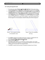
this line segment. For the second point, select the other point of the line (Figure 5).
First point
Second point
Figure 4. The line segment selected
is the translation vector.
4.
5.
6.
7.
8.
Figure 5. Result of the translation
with copy
Click Select to select the line segment that forms an angle of -60 degrees with the
horizontal. Press ESC to indicate that the selection has been made.
Choose GeometryÆEditÆIntersectionÆLine-line.
Select the two inner lines.
Click Yes to confirm that there is an intersection and that, therefore, the shortest
distance between the two entities is 0. The intersection between the two entities (lines)
creates a point. This point will be the tangential center.
Press ESC to indicate that the process of intersection between lines is finished.
78
CASE STUDY 2
Center of
Tangency
Figure 6. The auxiliary lines
NOTE: The Undo option allows you to undo the operations most recently carried out. If an
error is made, go to UtilitiesÆUndo; a window appears where you can select all the options to
be eliminated.
GID USER MANUAL
79
3. CREATING THE FIRST COMPONENT PART
In this section the entire model, except the T junction, will be created. The model to be created
is composed of two pipes forming a 60-degree angle. To start with, the first pipe will be created.
This pipe will then be rotated to create the second pipe.
3.1. Creating the profile
1.
2.
3.
Select the ok layer and click on Layer To use. From now on, all entities created will
belong to the ok layer.
Choose the Line option, located in GeometryÆCreateÆStraight line.
Enter the following points: (0, 11), (8, 11), (8, 31), (11, 31), (11, 11) and (15, 11). Press
ESC to indicate that the process of creating lines is finished.
Figure 7. Profile of one of the disks around the pipe
4.
From the Copy window, choose Lines and Translation. A translation defined by
points (0, 11) and (15, 11) will be made. In the Multiple copies option, enter 8 (the
number of copies to be added to the original). Select the lines that have just been
drawn.
Figure 8. The profile of the disks using Multiple copies
80
CASE STUDY 2
5.
6.
Choose Line, located in GeometryÆCreateÆStraight line. Select the last point on
the profile (at the right part of the profile) using the option Join Ctrl-a, which is in the
Contextual menu in the mouse menu. Now choose the option No join Ctrl-a. Enter
point (200, 11). Press ESC to finish the process of creating lines.
Again, choose the Line option and enter points (0, 9) and (200, 9). Press ESC to
conclude the process of creating lines (Figure 10).
Figure 9. Creating the lines of the profile
7.
8.
Figure 10. Copy of the vertical line
segment starting at the origin of
coordinates
From the Copy window, choose Lines and Translation. As the first and second points
of the translation, enter the points indicated in Figure 11. Click Select and select the
vertical line segment starting at the origin of coordinates. Press ESC.
Choose GeometryÆEditÆIntersectionÆMultiple lines. Select the last two lines
created and the vertical line segment coming down from the tangential center (see
Figure 12). Press ESC.
GID USER MANUAL
81
Figure 11. Selecting the lines to intersect
9.
Choose GeometryÆDeleteÆAll Types. (This tool may also be found in the GiD
Toolbox.) Select the lines and points beyond the vertical that passes through the
tangential center. Press ESC. They will be deleted and the result should look like that
shown in Figure 13.
Figure 12. Profile of the pipe and the auxiliary lines
82
CASE STUDY 2
3.2. Creating the volume by revolution
1.
2.
3.
Rotation of the profile will be carried out in two rotations of 180 degrees each. This
way, the figure will be defined by a greater number of points.
From the Copy window, select Lines and Rotation. Enter an angle of 180 degrees
and from the Do extrude menu, select Surfaces. The axis of rotation is that defined by
the line that goes from point (0, 0) to point (200, 0). Enter these two points as the First
Point and Second Point. Be sure to enter 1 in Multiple Copies.
Click Select. For an improved view when selecting the profile, click Off the “aux” layer.
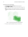
Press ESC when the selection is finished. The result should be that illustrated in Figure
14.
Figure 13. Result of the first step in the rotation (180 degrees)
4.
5.
6.
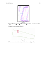
Repeat the process, this time entering an angle of –180 degrees.
To return to the side view (elevation), choose RotateÆPlane XY.
Choose RenderÆFlat from the mouse menu to visualize a more realistic version of the
model. Return to the normal visualization with RenderÆNormal. This option is more
comfortable to work with.
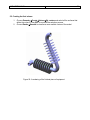
GID USER MANUAL
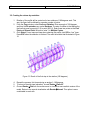
83
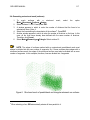
Figure 14. The pipe with disks, created by rotating the profile.
NOTE: To select the profile once the first rotation has been performed, first select all the
lines and then delete those that do not form the profile. Use the option RotateÆTrackball from
the mouse menu to rotate the model and make the process of selection easier.
84
CASE STUDY 2
3.3. Creating the union of the main pipes
1.
2.
3.
Choose the ZoomÆIn option from
the mouse menu. Magnify the right
end of the model.
Make sure the "aux" layer is
visible.
From the Copy window, select
Lines and Rotation. Enter an
angle of 120 degrees and from the
Do
extrude
menu,
select
Surfaces. Since the rotation may
be done in 2D, choose the option
Two Dimensions. The center of
the rotation is the tangential
center.
Figure 15. The magnified right end of
the model, and the lines to be selected
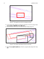
4.
Click Select and select the four lines that define the right end of the pipe (see Figure
16). Press ESC when the selection is finished.
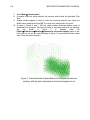
Figure 16. Result of the rotation
GID USER MANUAL
85
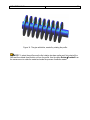
3.4. Rotating the main pipe
1.
2.
From the Copy window, select Surfaces and Rotation. Enter an angle of -60 degrees.
Since the rotation may be done in 2D, choose the Two Dimensions option. The center
of the rotation is the intersection of the axes, namely point (200, 0). Ensure the Do
Extrude menu is set to No.
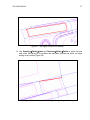
Click Select and select all the surfaces except those defining the elbow of the pipe.
Press ESC when the selection is finished.
Figure 17. Geometry of the two pipes and the auxiliary lines
86
CASE STUDY 2
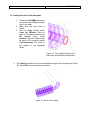
3.5. Creating the end of the pipe
1.
2.
3.
4.
From the Copy window, select Surfaces and Rotation. Enter an angle of 180
degrees. Since the rotation may be done in 2D, choose the option Two Dimensions.
The center of rotation is the upper right point of the pipe elbow. Make sure the Do
Extrude menu is set to No.
Click Select and select the surfaces that join the two pipe sections.
In the Move window, select Surfaces and Translation. The points defining the
translation vector are circled in Figure 19.
Click Select and select the surfaces to be moved. Press ESC. The result should be as
is shown in Figure 20.
Figure 18. The circled points define the
translation vector.
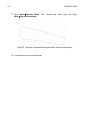
5.
6.
Figure 19. The final position of the translated
elbow.
Choose
GeometryÆCreateÆNURBS
surfaceÆBy contour and select the
four lines that define the opening of
the pipe (Figure 21). Press ESC.
From the Files menu, choose Save
in order to save the file. Enter a
name for the file and click Save.
Figure 20. Opening at the end of the pipe
GID USER MANUAL
87
4. CREATING THE SECOND COMPONENT PART: THE T JUNCTION
Now, an intersection composed of two pipe sections will be created in a separate file and the
surfaces will be trimmed. Then this file will be imported to the original model to create the entire
piece.
4.1. Creating one of the pipe sections
1.
2.
3.
4.
5.
Choose FilesÆNew, thus starting work in a new file.
Choose GeometryÆCreateÆPoint and enter points (0, 9) and (0, 11). Press ESC to
conclude the creation of points.
From the Copy window, select Points and Rotation. Enter an angle of 180 degrees
and from the Do extrude menu, select Lines. The axis of rotation is the x axis. Enter
two points defining the axis, one in First Point and the other in Second Point, for
example, (0, 0, 0) and (100, 0, 0) (Figure 22).
Click Select and select the two points just created.
Repeat the process, this time entering an angle of –180 degrees, thus creating the
profile of the pipe section with a second rotation of 180 degrees. The rotation could
have been carried out in only one rotation of 360 degrees. However, in the present
example, each circumference must be defined between two points (Figure 23).
Figure 21. The result of the first
180-degree rotation.
6.
7.
Figure 22. The combined result of the
first rotation and the second rotation of
–180 degrees, thus obtaining the
profile of the pipe section.
From the Copy window, choose Lines and Translation. In First Point and Second
Point, enter the points defining the translation vector. Since the pipe section must
measure 40 length units, the vector is defined by points (0, 0, 0) and (-40, 0, 0).
From the Do extrude menu, choose the Surfaces option.
88
CASE STUDY 2
8.
Click Select to select the lines that define the cross-section of the pipe. Press ESC to
conclude the selection process.
Figure 23. Creating a pipe by extruding circumferences
4.2. Creating the other pipe section
1.
2.
3.
4.
5.
6.
Choose GeometryÆCreateÆPoint and enter points (-20, 9) and
(-20, 11). Press ESC to conclude the creation of points.
From the Copy window, select Points and Rotation. Enter an angle of 180 degrees
and from the Do extrude menu, select Lines. Since the rotation can be done on the xy
plane, choose Two Dimensions. The center of rotation is the coordinates (-20, 0, 0).
Click Select and select the two points just created. Repeat the process, this time
entering an angle of -180 degrees.
From the Copy window, select Lines and Translation. In First Point and Second
Point enter the points defining the translation vector. Since this pipe section must also
measure 40 length units, the vector is defined by points (0, 0, 0) and (0, 0, 40).
From the Do extrude menu, select the Surfaces option.
Click Select to select the lines that define the cross-section of the second pipe. Press
ESC to conclude the selection.
Figure 24. A rendering of the two intersecting pipes
GID USER MANUAL
4.3. Creating the lines of intersection
1.
2.
3.
Choose GeometryÆEditÆIntersectionÆSurface-surface.
Select the outer surfaces of each pipe, thus forming the intersection of the two
surfaces selected.
Repeat the process to obtain the four lines of intersection.
Figure 25. Creating lines of intersection between the surfaces
89
90
CASE STUDY 2
4.4. Deleting surfaces and lines
1.
2.
Choose GeometryÆDeleteÆSurfaces and select the small surfaces inside the first
pipe. Press ESC to conclude the process of selection.
Choose GeometryÆDeleteÆLines. Select the lines defining the end of the second
pipe (foreground) that are still inside the first pipe (background). The result is shown in
Figure 27.
Figure 26. Final configuration after deleting surfaces and lines
GID USER MANUAL
91
4.5. Closing the volume
1.
2.
The model now has three outlets. The two farthest from the origin of coordinates must
be closed. The third will be connected to the rest of the piece when the T junction is
imported.
Choose GeometryÆCreateÆNURBS SurfaceÆBy contour and then select the lines
defining the outlet in the foreground of Figure 28. Press ESC (see Figure 28).
Figure 27. Creating a NURBS surface to close the outlet in the foreground
3.
4.
Repeat the process for the other outlet to be closed.
From the Files menu, select Save to save the file. Enter a name for the file and click
Save.
92
CASE STUDY 2
5. IMPORTING THE T JUNCTION TO THE MAIN FILE
The two parts of the model have been drawn. Now they must be joined so that the final volume
may be created and a mesh of the volume may be generated.
5.1. Importing a GiD file
1.
2.
3.
4.
Choose Read from the Files menu. Select the file where the first part, created in
section 3, was saved. Click Open.
Choose FilesÆImportÆInsert GiD geometry from the menu. Select the file where
the second part, created in section 4, was saved. Click Open.
The T junction appears. Bear in mind that the lines which define the end of the first
pipe (background) of the T junction, and which have been imported, were already
present in the first file. Notice that the lines overlap. This overlapping will be remedied
by collapsing the lines.
Choose the option GeometryÆEditÆCollapseÆLines. Select the overlapping lines
and press ESC.
Figure 28. Importing the T junction file to the main file.
Some points are duplicated and must be collapsed.
GID USER MANUAL
93
5.2. Creating the final volume
1.
2.
Choose GeometryÆCreateÆVolumeÆBy contour and select all the surfaces that
define the volume. Press ESC to conclude the selection process.
Choose RenderÆSmooth to visualize a more realistic version of the model.
Figure 29. A rendering of the finished piece of equipment
94
CASE STUDY 2
6. GENERATING THE MESH
Now that the model is finished, it is ready to be meshed. The mesh will be generated using
Chordal Error in order to achieve greater accuracy in the discretization of the geometry. The
chordal error is the distance between the element generated by the meshing process and the
real profile of the model. By selecting a sufficiently small chordal error, the elements will be
smaller in the zones with greater curvature.
6.1. Generating the mesh using Chordal Error
1.
2.
3.
4.
5.
6.
7.
8.
9.
Choose the option MeshÆUnstructuredÆSizes by Chordal error.
Enter 1 for the minimum element size.
Enter 15 for the maximum element size.
Enter 0.2 for the chordal error.
Choose MeshÆGenerate mesh.
A window opens in which to enter the maximum element size of the mesh to be
generated. Leave the default value provided by GiD unaltered and click OK.
When the meshing process is finished, a window appears with information about the
mesh that has been generated. Click OK to visualize the mesh.
Choose MeshÆView Mesh Boundary to see only the contour of the volumes meshed
but not the interiors.
The visualization may be rendered using the various options in the Render menu,
located in the mouse menu.
Figure 30. The mesh generated for the piece
NOTE: By default GiD corrects element size depending on the form of the entity to mesh.
This correction option may be deactivated or reactivated in the Meshing card in the
Preferences window under the option Automatic correct sizes.
GID USER MANUAL
95
6.2. Generating the mesh by assignment of sizes on surfaces
1.
2.
3.
4.
5.
6.
Choose MeshÆUnstructuredÆAssign sizes on surfaces. A window opens in which
to enter the element size for the surfaces to be selected. Enter size 1.
Select the surfaces of the elbow.
Choose MeshÆGenerate mesh.
A window appears asking whether the previous mesh should be eliminated. Click Yes.
Another window appears in which the maximum element size should be entered.
Leave the default value provided by GiD unaltered and click OK.
Choose MeshÆView Mesh Boundary to see only the contour of the meshed volumes
but not the interiors (Figure 32).
Figure 31. The mesh with a concentration of elements on the surfaces of the elbow
7.
A greater concentration of elements has been achieved on the selected surfaces.
96
ASSIGNING ELEMENT SIZES
ASSIGNING ELEMENT SIZES FOR GENERATING THE
MESH
The objective of this example is to mesh a mechanical piece using the various options in GiD for
assigning sizes to elements, and the different surface meshers available. In this example a
mesh is generated for each of the following methods for assigning sizes, using different surface
meshers:
•
•
•
•
Assigning sizes around points
Assigning sizes around lines
Assigning sizes on surfaces
Assigning sizes with Chordal Error
GID USER MANUAL
97
1. INTRODUCTION
In order to carry out this example, start by opening the project “ToMesh4.gid”. This project
contains a geometry that will be meshed using four different methods, each one resulting in a
different density of elements in certain zones.
1.1. Reading the initial project
1.
2.
3.
4.
5.
In the Files menu, select Read. Select the project “ToMesh4.gid” and click Open.
The geometry appears on the screen. It is a set of surfaces.
1
Select RenderÆFlat from the mouse menu .
Select RotateÆTrackball from the mouse menu. (This tool is also available within the
GiD Toolbox.) Make several changes in the perspective so as to get a good idea of the
geometry of the object.
Finally, return to the normal visualization, selecting RenderÆNormal. This mode is
more user-friendly.
Figure 1. Contents of the project “ToMesh4.gid”.
1
The mouse menu appears when the right mouse button is clicked.
98
ASSIGNING ELEMENT SIZES
GID USER MANUAL
99
2. ELEMENT- SIZE ASSIGNMENT METHODS
GiD automatically corrects element sizes according to the shape of the entity to be meshed and
its surrounding entities. This default option may be deactivated and reactivated by going to the
2
3
Mesh menu, selecting Preferences , and then Automatic correct sizes .
Sometimes, however, this type of correction is not sufficient and it is necessary to indicate
where on the mesh greater accuracy is needed. In these cases, GiD offers various options and
methods allowing sizes to be assigned to elements. Five examples are shown to illustrate the
default method and the four other methods.
2.1. Assignment using default options
1.
2.
3.
Select MeshÆGenerate Mesh.
A window appears showing the maximum element size. Leave this default size
unaltered and click OK.
A meshing process window opens. Then another window appears with information
about the mesh generated. Click OK to visualize the mesh (see Figure 2).
Figure 2. Meshing by default.
2
3
The Preferences option can also be found in the Utilities menu.
Automatic correct sizes automatically executes the options Assign sizesÆBy
geometry and Assign sizesÆCorrect sizes.
100
ASSIGNING ELEMENT SIZES
Note that in the zone highlighted in Figure 3, elements are smaller than in the rest of the model.
This is because of the shape of the surface placed there. When all meshing preferences are set
to their default levels, as for this example, the RFAST surface mesher is used. In this way,
geometrical entities are meshed hierarchically: first of all lines are meshed, then the surfaces,
and finally the volumes. The line elements size depends on the shape of surfaces (as can be
seen in this example). Later on we will see an example using RJUMP mesher, where element
sizes are distributed differently.
Figure 3. Meshing by default. Zone where elements are smaller because of the
surface shape.
GID USER MANUAL
101
2.2. Assignment around points
1.
2.
3.
4.
5.
Select MeshÆUnstructuredÆAssign size on points. A window appears in which to
enter the element size around the points to be chosen. Enter 0.1 and click OK.
4
Select the point indicated in Figure 4. Press ESC to indicate that the selection of
points is finished.
Select MeshÆGenerate Mesh.
A window opens asking whether the previous mesh should be eliminated. Click Yes.
GiD then asks you to enter the maximum element size. Leave the default value
unaltered and click OK.
Figure 4. Geometry of the model. The point
around which the mesh will be concentrated.
6.
7.
8.
4
Figure 5. The mesh with a concentration of
elements around the point.
A concentration of elements appears around the chosen point, given the selected size
(0.1) of these elements (see Figure 5).
Go to Utilities and open Preferences. Click Meshing. In the window that appears
there is the option Unstructured Size Transitions. This option defines the transition
gradient of element sizes (size gradient), whose values are between 0 and 1. The
greater the size gradient, the greater the change in space. To test this, enter the value
0.4 and click Accept.
Again, select MeshÆGenerate Mesh.
Instead of pressing the ESC key, the center mouse button or the mouse wheel can
also be used.
102
ASSIGNING ELEMENT SIZES
9. A window opens asking whether the previous mesh should be eliminated. Click Yes.
10. GiD then asks you to enter the maximum element size. Leave the default value
unaltered and click OK.
Figure 6. Mesh with the elements concentrated around a point, with a
size gradient of 0.8.
11. The size gradient (0.4) results in a higher density around the point (see Figure 6).
12. Now go back and enter 0.6 in Unstructured Size Transitions. This will result in a
mesh more suitable for our objectives. Click Accept.
GID USER MANUAL
103
2.3. Assignment around lines
1.
2.
3.
4.
5.
Select MeshÆUnstructuredÆAssign size on lines. In the window that appears,
enter the size of the elements around the lines that will be chosen. Enter 0.5 and click
OK.
Select the lines defining the base of the prism (i.e. lines 1, 2, 3, 4 and 40). To see
entity numbers select Label from the mouse menu or from the View menu. If you wish
geometrical entity labels to be displayed, the view mode has to be set to Geometry
using ViewÆModeÆGeometry (this option may also be found in the GiD Toolbox),
and the render mode must be set to Normal. Press ESC.
Select MeshÆGenerate Mesh.
A window opens asking if the previous mesh should be eliminated. Click Yes.
Another window appears in which you may enter a maximum element size. Leave the
default value unaltered and click OK. This results in a high concentration of elements
around the chosen lines, given that the selected element size (0.5) is much smaller
than that of the rest of the elements in the model (see Figure 7).
Figure 7. Mesh with a concentration of elements around lines.
104
ASSIGNING ELEMENT SIZES
2.4. Assignment on surfaces
1.
2.
3.
4.
5.
Select MeshÆUnstructuredÆAssign size on surfaces. In the window that appears,
enter the size of the elements to be assigned on the surfaces that will be chosen. Enter
0.5 and click OK.
Select the triangular surface resulting from the section of one of the vertexes of the
prism (surface number 1). Press ESC.
Select MeshÆGenerate Mesh.
A window opens asking if the previous mesh should be eliminated. Click Yes.
Another window appears in which you can enter the maximum element size. Leave the
default value unaltered and click OK. This results in a high concentration of elements
on the chosen surface; due to the value selected (0.5) (see Figure 8).
Figure 8. Mesh with a concentration of elements on a surface.
GID USER MANUAL
105
2.5. Assignment with Maximum Chordal Error
1.
2.
3.
4.
5.
6.
7.
Select MeshÆUnstructuredÆSizes by chordal error….
GiD asks for the minimum element size. Enter 0.1.
GiD asks for the maximum element size. Enter 10.
Enter the chordal error. This error is the maximum distance between the element
generated and the real object (geometry). Enter 0.05 and press OK.
Select MeshÆGenerate Mesh.
A window opens asking if the previous mesh should be eliminated. Click Yes.
Another window appears in which you can enter a maximum element size. Leave the
default value unaltered and click OK. This results in a high concentration of elements
in curved areas. Now our approximation is significantly improved (see Figure 9).
Figure 9. Mesh using sizes assignment by chordal error. Here, there
is a greater concentration of elements in the curved zones.
106
ASSIGNING ELEMENT SIZES
3. RJUMP MESHER
3.1. RJump default options
The RJump mesher is a surface mesher that meshes patches of surfaces (in 3D space) and is
able to skip the inner lines of these patches when meshing. By default, the RJump mesher skips
the contact lines between surfaces that are tangent enough, and points between lines that are
tangent enough. By selecting MeshÆDrawÆ Skip entities (Rjump), the entities that RJump is
going to skip and the ones that it is not going to skip are displayed in different colors. In this
chapter we will see the properties of this mesher.
1.
2.
3.
4.
5.
6.
Select MeshÆReset mesh data to reset all mesh sizes introduced previously.
A window appears advising that all the mesh information is going to be erased. Press
OK.
Go to Utilities and open Preferences. Click Meshing. In the window that appears you
can choose between the three surface meshers available in GiD (RFast, RSurf and
RJump). Select RJump mesher. Click Accept.
Select MeshÆGenerate Mesh.
A window opens asking if the previous mesh should be eliminated. Click Yes.
Another window appears in which you can enter a maximum element size. Leave the
default value unaltered and click OK. This results in a mesh where contact lines
between surfaces that are tangent enough do not have nodes; contact points between
lines tangent enough are also skipped when meshing (see Figure 10).
Figure 10. Mesh using the RJump mesher.
GID USER MANUAL
107
Note that the smaller elements shown in Figure 3 do not appear in this mesh, because of the
properties this mesher.
7.
8.
9.
10.
11.
12.
13.
Using the RJump mesher it is possible to assign sizes to different entities. As an
example, select MeshÆUnstructuredÆSize by chordal error….
GiD asks for the minimum element size. Enter 0.1.
GiD asks for the maximum element size. Enter 10.
Enter the chordal error. This error is the maximum distance between the element
generated and the real object. Enter 0.05 and press OK.
Again, select MeshÆGenerate Mesh.
A window opens asking if the previous mesh should be eliminated. Click Yes.
Another window appears in which you can enter a maximum element size. Leave the
default value unaltered and click OK. This results in a high concentration of elements
in curved areas, without the nodes in the lines and points that mesher skips. Now our
approximation is significantly improved (see Figure 11).
Figure 11. Mesh using the RJump mesher and assigning sizes
by chordal error.
108
ASSIGNING ELEMENT SIZES
3.2. Force to mesh some entity
If there is a line or a point that the RJump mesher would usually skip, but that you wish to be
meshed, you can specify the entity so that it is not skipped. As an example, we will force Rjump
to mesh line number 43, in order to concentrate elements around point number 29, as it was
done in chapter 2.2.
1.
2.
Select MeshÆMesh criteriaÆNo skipÆlines, and select line number 43. Press ESC.
Select MeshÆDrawÆ Skip entities (Rjump) to display the entities that will and will
not be skipped in different colors. As is shown in Figure 12, line 43 will now not be
skipped; the rest of the lines are unaffected, and RJump will either skip or mesh them
according to its criteria.
Figure 12. Entities that will be skipped and not skipped using the
RJump mesher.
3.
4.
5.
6.
Select MeshÆUnstructuredÆAssign size on points. A window appears in which to
enter the element size around the points to be chosen. Enter 0.1 and click OK.
Select the point indicated in Figure 4 (point number 29). Press ESC to indicate that the
selection of points is finished.
Select MeshÆGenerate Mesh.
A window opens asking if the previous mesh should be eliminated. Click Yes.
GID USER MANUAL
7.
109
Another window appears in which you can enter a maximum element size. Leave the
default value unaltered and click OK. This results in a mesh like the one obtained
before (in Figure 10), but with high concentration of elements around point number 29.
Note that there are nodes on line number 43 because we have forced RJump not to
skip this line (see Figure 13).
Figure 13. Mesh using the RJump mesher, assigning sizes by
chordal error and forcing an entity to be meshed.
In this last example we have forced the mesher not to skip an entity, but it may be interesting in
some models to allow the mesher only to skip a few entities, meshing almost all or them. In this
case, a different surface mesher can be selected (in the Preferences window). One option is
the RSurf mesher which meshes everything except the entities that you ask it to skip, using the
MeshÆMesh criteriaÆSkip command. Here, because RJump is not selected, no entity will be
skipped automatically according to tangency with neighboring entities. The next example shows
how to work with this mesher.
8.
9.
Select MeshÆReset mesh data to reset all mesh sizes introduced previously.
A window opens advising that all the mesh information is going to be erased. Press
OK.
10. Go to Utilities and open Preferences. Click Meshing. In the window that appears you
can choose between the three surface meshers available in GiD (RFast, RSurf and
RJump). Select the RSurf mesher. Click Accept.
11. Select MeshÆMesh criteriaÆSkipÆlines, and select lines 48 and 53. Press ESC.
12. Select MeshÆGenerate Mesh.
110
ASSIGNING ELEMENT SIZES
13. A window opens asking if the previous mesh should be eliminated. Click Yes.
14. Another window appears in which you can enter a maximum element size. Leave the
default value unaltered and click OK. The result is a mesh similar to the first example
obtained in chapter 2 (see Figure 2), but the smaller elements highlighted in Figure 3
do not appear because lines 48 and 53 (which were meshed before) are now skipped
when meshing (see Figure 14).
Figure 14. Mesh using the RSurf mesher, with
some lines skipped.
GID USER MANUAL
111
METHODS FOR GENERATING THE MESH
The objective of this example is to mesh a model using the various options available in GiD for
controlling the element type in structured, semi-structured and unstructured meshes. It also
presents how to concentrate elements and control the distribution of mesh sizes.
The six methods covered are:
•
•
•
•
•
•
Generating a mesh using tetrahedra
Generating a volume mesh using points
Generating a mesh using quadrilaterals
Generating a structured mesh on surfaces and volumes
Generating a semi-structured volume mesh
Generating a mesh using quadratic elements
112
METHODS FOR GENERATING THE MESH
1. INTRODUCTION
In order to carry out this example, start from the project "ToMesh3.gid". This project contains a
geometry that will be meshed using different types of elements.
1.1. Reading the initial project
1.
2.
3.
In the Files menu, select Read. Select the project “ToMesh3.gid” and click Open.
The geometry appears on the screen. It is a set of surfaces and three volumes. Select
RenderÆFlat from the mouse menu1 or from the View menu. In Figure 1 shows the
geometrical model loaded.
Select RotateÆTrackball from the mouse menu. (This option is also available in the
GiD Toolbox.) Make several changes in the perspective so as to get a good idea of the
geometry involved.
Figure 1. Contents of the project “ToMesh3.gid”.
4.
1
Finally, return to the normal visualization RenderÆNormal. This mode is more userfriendly.
The mouse menu appears when the right mouse button is clicked.
GID USER MANUAL
113
2. GENERATING THE MESH - TYPES OF MESHES
Using GiD the mesh may be generated in different ways, depending on the needs of each
2
project. The two basic types of meshes are the structured mesh and the unstructured mesh.
For volumes only there is one additional type, the semi-structured3 mesh. For all these types of
mesh a variety of elements may be used (linear ones, triangles, quadrilaterals, tetrahedra,
hexahedra, prisms, spheres or points). In this tutorial you will become familiarized with the
mesh-generating combinations available in GiD.
2.1. Generating the mesh by default
1.
2.
3.
4.
5.
2
Select MeshÆGenerate mesh.
A window comes up in which to enter the maximum element size for the mesh to be
generated. Leave the default value unaltered and click OK.
A meshing process window comes up. Then another window appears with information
about the mesh generated. Click OK to visualize the mesh.
The result is the mesh in Figure 2. There are various surfaces and volumes. By default,
mesh generation in GiD obtains unstructured meshes of triangles on surfaces and
tetrahedra on volumes.
Select RenderÆFlat to see the mesh in render mode. As is shown in Figure 3, volume
meshes are represented a little bit differently from surface meshes, although in both
cases triangles are shown. If the triangles you see are the boundary of a volume mesh,
they are shown with black edges that are thicker than surface meshes triangles. If the
triangles form a boundary volume mesh and, at the same time, a triangle surface mesh
(this can be obtained if surfaces are selected with the option MeshÆMesh
criteriaÆMeshÆSurfaces), the wider edges are colored with the color of the surface
layer. Examples of these different kinds of render are shown in Figure 3.
A structured mesh is one in which each node is connected to a constant number of elements.
A semi-structured volume mesh is one in which you can distinguish a fixed structure in one
direction, i.e. there is a fixed number of divisions. However, within each division the mesh need
not be structured. This kind of mesh is only practical for topologically prismatic volumes.
3
114
METHODS FOR GENERATING THE MESH
Figure 2. Generating the mesh by default.
a)
b)
c)
Figure 3. Different render styles: a) surface mesh, b)
volume mesh, c) surface mesh and volume mesh together
(surface layer is red and volume layer is blue).
GID USER MANUAL
115
2.2. Generating the mesh using points
1.
2.
3.
4.
Select MeshÆElement typeÆOnly points. Select volume number one and press
ESC4. To see entity numbers select Label from the mouse menu or from the View
menu. If you wish the geometrical entity labels to be displayed, the view mode needs
to be changed to Geometry using ViewÆModeÆGeometry (this option may also be
found in the GiD Toolbox). Select RenderÆNormal to see the labels.
Select MeshÆGenerate mesh.
A window comes up asking whether the previous mesh should be eliminated. Click
Yes.
Another window appears in which to enter the maximum element size. Leave the
default value unaltered and click OK. The result is a mesh as illustrated in Figure 4.
Figure 4. Generating a mesh on a volume using points.
5.
4
Now volume number one is meshed using only the generated nodes.
Instead of pressing the ESC key, the center mouse button or the mouse wheel can also be
used.
116
METHODS FOR GENERATING THE MESH
2.3. Generating the mesh using quadrilaterals
1.
2.
3.
4.
Select MeshÆElement typeÆQuadrilateral. Select surface number 10.
Select MeshÆGenerate mesh.
A window comes up asking whether the previous mesh should be eliminated. Click
Yes.
Another window appears in which the maximum element size can be entered. Leave
the default value unaltered and click OK. The result will be the mesh illustrated in
Figure 5.
Figure 5. An unstructured mesh generated using quadrilaterals.
5.
The surface is meshed with quadrilaterals, forming an unstructured mesh.
GID USER MANUAL
117
2.4. Generating a structured mesh (surfaces)
1.
2.
3.
4.
5.
6.
To
mesh
surfaces
with
a
structured
mesh,
select
the
option
MeshÆStructuredÆSurfacesÆAssign.
Select surfaces 11 and 12 and press ESC.
A window appears in which to enter the number of divisions that the lines to be
selected will have. Enter 4.
5
Select the lines defining the boundaries of the surfaces . Press ESC.
Another window appears in which to enter the number of divisions on the lines. In this
case, all the lines have already been defined with the same number of divisions.
Therefore, click Cancel.
Select MeshÆElement typeÆTriangle. Select surface 12.
NOTE: The edges of surfaces meshed with an unstructured quadrilateral mesh must
always be divided into an even number of segments. So, if these surfaces share edges with a
structured surface mesh, the edges of the structured surface must also be divided into an even
number of segments. In this example, therefore, lines are divided into 4 segments.
Figure 6. Structured mesh of quadrilateral and triangular elements on surfaces.
5
When selecting a line, GID automatically selects all lines parallel to it.
118
METHODS FOR GENERATING THE MESH
7.
8.
Select MeshÆGenerate mesh.
A window comes up asking whether the previous mesh should be eliminated. Click
Yes.
9. Another window appears in which to enter the maximum element size. Leave the
default value unaltered and click OK. The result is the mesh shown in Figure 6.
10. As seen in Figures 6 and 7, GiD can obtain surface structured meshes made of
quadrilaterals or triangles. There are two kinds of structured mesh that use triangles:
the
one
shown
in
Figure
6
is
obtained
when
the
UtilitiesÆPreferencesÆMeshingÆSymmetrical structured triangles option is set.
If this option is not set, the mesh presented in Figure 7 is produced (with fewer nodes
than if using the previous option).
Figure 7. Structured mesh of quadrilateral and triangular elements on
surfaces, with the option Symmetrical structured triangles not set.
GID USER MANUAL
119
2.5. Generating structured meshes (volumes)
1.
2.
3.
4.
5.
6.
To
mesh
volumes
with
a
structured
mesh,
select
the
option
MeshÆStructuredÆVolumes.
6
Select volumes 1 and 2 and press ESC .
A window appears in which to enter the number of divisions that the lines to be
selected will have. Enter 6.
Select lines of both volumes parallel to the X- and Z-axes. GiD automatically selects all
the lines in each volume parallel to these in order to create the structured mesh. Press
ESC.
Another window appears in which to enter the number of divisions on the lines. Divide
the lines parallel to the Y-axis into 8 segments. Enter 8 and click OK.
Select an edge of volume 1 or 2 parallel to the Y-axis and press ESC. Again, the linedivision window comes up. Since we have already finished the assignments, click
Cancel.
Figure 8. Structured volume mesh of hexahedra and tetrahedra.
6
Only volumes that are topologically cubic can be meshed with a structured mesh.
120
METHODS FOR GENERATING THE MESH
7.
For structured volumes, GiD generates hexahedron meshes by default, but tetrahedron
structured meshes can also be assigned. Select MeshÆElement typeÆTetrahedra
and then select volume number 2.
8. Select MeshÆGenerate mesh.
9. A window appears asking whether the previous mesh should be eliminated. Click Yes.
10. Another window comes up in which to enter the maximum element size. Leave the
default value unaltered and click OK. The result is the mesh shown in Figure 8.
11. GiD can obtain volume structured meshes made of hexahedra, tetrahedra or prisms.
As can be seen in Figures 8 and 9, there are two kinds of tetrahedron structured mesh:
the
one
shown
in
Figure
8
is
obtained
when
the
option
UtilitiesÆPreferencesÆMeshingÆSymmetrical structured tetrahedra is set. If this
option is not set, the mesh presented in Figure 9 is produced (with fewer nodes than if
using the previous option; also, it is not topologically symmetrical).
Figure 9. Structured volume mesh of tetrahedra with the option Symmetrical
structured tetrahedra not set.
GID USER MANUAL
121
2.6. Generating semi-structured meshes (volumes)
1.
2.
3.
4.
5.
6.
7.
To mesh volumes with a semi-structured mesh, select the option
MeshÆSemiStructuredÆVolumes.
A window appears in which to enter the number of divisions for the direction in which it
is structured (the prismatic one). Enter 8.
7
Select volume 3 and press ESC . As volume 3 is prismatic in one direction only (i.e.
parallel to Y-axis) GiD will automatically detect this fact and will select it to be the
direction in which the semi-structured volume mesh is structured.
Another window appears in which to enter the number of divisions in the direction of
the structure. In this case we do not want to select any more volumes, so click Cancel.
Select MeshÆGenerate mesh.
A window appears asking whether the previous mesh should be eliminated. Click Yes.
Another window appears in which to enter the maximum element size. Leave the
default value unaltered and click OK. The result is the mesh shown in Figure 10.
Figure 10. Semi-structured volume mesh of tetrahedra.
7
Only volumes that are topologically prismatic can be meshed with a semi-structured mesh.
122
METHODS FOR GENERATING THE MESH
As can be seen, volume 3 has been meshed with tetrahedra. Semi-structured volumes are
meshed with prisms, by default. However, in this case it was not possible because of volume 2,
which has tetrahedra assigned and shares one surface with volume 3. In the following steps a
hexahedron mesh is produced.
8.
9.
10.
11.
12.
Select MeshÆElement typeÆHexahedra.
Select volumes 2 and 3 and press ESC.
Select MeshÆGenerate mesh.
A window opens asking whether the previous mesh should be eliminated. Click Yes.
Another window appears in which to enter the maximum element size. Leave the
default value unaltered and click OK. The result is the mesh shown in Figure 11.
Figure 11. Semi-structured volume mesh of hexahedra.
In case of volume number 3 there is only one direction in which it can possibly be structured (i.e.
in the direction of the prism). If the volume is prismatic in more than one direction, there are two
ways
to
choose
between
them:
selecting
one
top
surface
(MeshÆSemiStructuredÆSetÆMaster surface) or the direction of the structure
(MeshÆSemiStructuredÆSetÆStructured direction). The following example explains this
procedure.
13. Select the option MeshÆSemiStructuredÆVolumes.
14. A window opens in which to enter the number of divisions in the structured direction
(prismatic). Enter 6.
15. Select volume 1 and press ESC.
16. Select MeshÆSemiStructuredÆSetÆStructured direction.
GID USER MANUAL
123
8
17. Select one line parallel to the X-axis of volume number 1 (for example line number 11)
and press ESC.
18. Select MeshÆUnstructuredÆAssign EntitiesÆSurfaces.
19. Select surfaces 1 and 6 and press ESC9.
20. Select MeshÆGenerate mesh.
21. A window opens asking whether the previous mesh should be eliminated. Click Yes.
22. Another window appears in which to enter the maximum element size. Leave the
default value unaltered and click OK. The result is the mesh shown in Figure 12.
Figure 12. Semi-structured volume mesh of prisms and hexahedra.
NOTE: As can be seen, by selecting different element types for different geometrical
entities, several kinds of meshes can be generated. Remember always to take care over the
compatibility between element types in shared geometrical entities.
8
Volume number one have not been selected as semi-structured, but GiD will assign this mesh
criteria to it automatically when selecting one of its lines to be a structured direction.
9
It’s necessary to set one top surface of the volume “unstructured” because, otherwise, volume
1 will become totally structured. It is because all contour surfaces of this volume have been
assigned as structured automatically when assigning previously this kind of mesh to the volume
(step 2 of chapter 2.5).
124
METHODS FOR GENERATING THE MESH
2.7. Concentrating elements and assigning sizes
1.
2.
3.
4.
5.
6.
Select MeshÆStructuredÆLinesÆConcentrate elements.
Select some structured lines, for example lines 3 and 23. Press ESC.
A window comes up in which to enter two values for the concentration of elements.
Positive values concentrate the elements and negative values spread them. Enter 1 as
10
Start Weight and –0.5 as End Weight .
Select MeshÆGenerate mesh.
A window opens asking whether the previous mesh should be eliminated. Click Yes.
Another window appears in which to enter the maximum element size. Leave the
default value unaltered. The result is the mesh shown in Figure 13.
Figure 13. Concentration of elements on lines 3 and 23.
It is also possible to assign sizes to geometrical entities, so that mesh elements can be
concentrated in certain zones. In the following steps some examples are given.
10
Start Weight and End Weight refer to the start point and end point of the line, oriented as it is
drawn when you select it.
GID USER MANUAL
7.
8.
9.
10.
11.
12.
13.
14.
15.
16.
17.
125
Select MeshÆUnstructuredÆAssign sizes on points.
A window appears in which to enter the size to be assigned to points. Enter “0.1”.
Select point number 11 and press ESC.
Another window appears in which to enter the size to be assigned to points. In this
case, we do not want to assign sizes to any other points, so click Cancel.
Select MeshÆUnstructuredÆAssign sizes on lines.
A window appears in which to enter the size to be assigned to lines. Enter “0.5”.
Select line number 21 and press ESC.
Another window appears in which to enter the size to be assigned to lines. In this case,
we do not want to assign sizes to any more lines, so click Cancel.
Select MeshÆGenerate mesh.
A window appears asking whether the previous mesh should be eliminated. Click Yes.
Another window appears in which the maximum element size should be entered.
Leave the default value unaltered. The result is the mesh shown in Figure 14.
Figure 14. Unstructured size assigned in point 11 and line 21.
126
METHODS FOR GENERATING THE MESH
2.8. Generating the mesh using quadratic elements
1.
2.
Select ZoomÆIn from the mouse menu (this option may also be found in the GiD
Toolbox or in the View menu). Enlarge one area of the mesh (e.g. the zone near point
number 3).
Select LabelÆAll inÆPoints. The result is shown in Figure 15.
Figure 15. Each number identifies a node. There is a
node for each element vertex.
3.
The node identifiers created by generating the mesh appear on the screen. There is
one identifier for each vertex of each element.
4. Select MeshÆQuadratic elementsÆQuadratic.
5. Select MeshÆGenerate mesh.
6. A window opens asking whether the previous mesh should be eliminated. Click Yes.
7. Another window appears in which the maximum element size should be entered.
Leave the default value unaltered and click OK.
8. Once the mesh has been generated, select LabelÆAll inÆPoints. The result is
shown in Figure 16. Now, there are not only nodes at the vertices, but also at the
midpoints of the edges of the elements.
9. Select MeshÆQuadratic elementsÆQuadratic9.
10. Select MeshÆGenerate mesh.
NOTE: By default GiD meshes with first degree (linear) elements. To find out which mode
GiD is working in, select MeshÆQuadratic elements, and it is the flagged option.
GID USER MANUAL
127
Figure 16. Each number identifies a node. There is a node at each element
vertex and at the midpoint of each edge.
11. A window opens asking whether the previous mesh should be eliminated. Click Yes.
12. Another window appears in which the maximum element size should be entered.
Leave the default value unaltered.
13. Select LabelÆAll inÆPoints (see Figure 17).
14. Notice that the four-sided elements (quadrilaterals) also have a node in the center, in
addition to the nodes at the vertices and midpoints of the edges. Similarly, hexahedra
also have a node at their center point.
Figure 17. Each number identifies a node. There is a node at each vertex, at
the midpoint of each edge and in the center of quadrilaterals and hexahedra.
128
POSTPROCESSING A RATCHET WHEEL
A POST-PROCESS CASE STUDY
POST-PROCESSING A RATCHET WHEEL
The objective of this case study is to run a post-process analysis of a steel ratchet wheel
subjected to a set of forces. We will observe the stresses on the material and the resulting
deformations.
The analysis is carried out in four steps:
•
•
•
•
Redefining the part
Entering conditions and materials
Generating the mesh for the entire part and calculating the stresses
Visualizing the results
By the end of this study, you should be able to run a structural analysis of a model subjected to
external forces and visualize the results in GiD Post-process.
GID USER MANUAL
129
1. INTRODUCTION
The model in this study will be the one created in Tutorial 1, located in the file “pieza.gid”. The
geometry in this file will be the object of this post-process study.
1
In order to follow this tutorial, the calculating module Ramsolid must be installed. To install
Ramsolid, select DataÆProblem typeÆInternet Retrieve. A window with the available
modules will appear. Select RamSeries Windows, which contains Ramsolid, and click
Retrieve Problem type to install it.
NOTE: You can find the finished model on the GiD CD-ROM or on the GiD web page:
http://www.gidhome.com/support.
1
For further information on Ramsolid, consult www.compassis.com
130
POSTPROCESSING A RATCHET WHEEL
1.1. Reading the initial file
1.
2.
3.
From the Files menu, choose the option Read. Select the file named “pieza.gid” and
click Open. The geometry in Figure 1 appears on the screen.
Choose RenderÆFlat from the mouse menu.
Choose RotateÆTrackball from the mouse menu. (This tool is also located in the GiD
Toolbox.) Make a few changes to the perspective in order to get an idea of the
geometry under study.
Figure 1. Contents of the “pieza.gid” file
4.
Return to the normal visualization by selecting RenderÆNormal. This mode is more
comfortable to work with.
GID USER MANUAL
131
2. CREATING A SINGLE VOLUME
When you carry out a stress test which involves the different volumes that define a structural
solid, Ramsolid requires these volumes to share the surfaces of interaction, that is, these
surfaces must belong to both volumes.
Since the geometry of this study is formed by two volumes with separate surfaces, the volumes
must be connected. To do this, we will delete the existing volumes (those of the axle and the
wheel) and create one new volume as a union of the two.
2.1. Deleting volumes and surfaces
1.
2.
3.
2
Choose GeometryÆDeleteÆVolumes .
Select the two volumes in the file. Press ESC3.
Choose GeometryÆDeleteÆSurfaces2. Select4 the surfaces shown in Figure 2 and
Figure 3 and press ESC.
4.
Figure 2. The axle surfaces to select
2
Figure 3. The wheel surfaces to select
This option may also be found in the GiD Toolbox.
Pressing the ESC key is equivalent to clicking the center mouse button.
4
To facilitate the selection of these surfaces, deactivate any unnecessary layers.
3
132
POSTPROCESSING A RATCHET WHEEL
Figure 4. The result after deleting volumes and surfaces
2.2. Creating new surfaces and the final volume
1.
Choose the option UtilitiesÆCopy; the Copy window appears. In this window choose
Translation and Lines. The translation vector of the required translation is the line
segment shown in Figure 5. Enter as First Point and Second Point the two points
defining this vector. These points are also shown in Figure 5.
First Point
Second
Point
Figure 5. The translation vector and the points that define it
GID USER MANUAL
2.
3.
133
Choose the option Surfaces from the Do Extrude menu in the Copy window.
Verify that the “Duplicate entities” option is unchecked, and then click Select and
select the lines defining the hole in the wheel. Press ESC. (See Figure 6.)
Figure 6. Visualization of the new surfaces created at one end of the axle
4.
5.
Repeat the process to create the surfaces at the other end of the axle.
When all the surfaces have been created, thus defining a new part (axle and wheel as
one), choose GeometryÆCreateÆVolumeÆBy contour2 and select all the surfaces.
Press ESC.
Figure 7. Visualization of the new volume
6.
7.
Choose GeometryÆDeleteÆLines and select all the lines in the model. Press ESC.
Only the lines not contained by the volume will be deleted.
134
POSTPROCESSING A RATCHET WHEEL
3. CALCULATING WITH RAMSOLID
Since this is a 3D problem, the calculating module “Ramsolid 5.5” will be used to run it. First we
must load the problem type ramsolid which is located in DataÆProblem type.
Note: Your Ramsolid version can be different to the related 5.5, but the steps to follow will be
analogous.
The object of the study is a ratchet wheel that permits rotation of the axle in only one direction.
The aim is to study how the part behaves when subjected to external forces, especially when
the wheel is in equilibrium. In this condition, rotation is blocked by the pole, which resists the
rotating force coming from the axle. At the same time, the pole exerts an equal and opposite
force on one of the teeth. This system is illustrated in Figure 8.
A
B
Figure 8. Ratchet wheel and (in red) pole
In order to simulate this condition, the following simplification will be made: the ends of the axle
will be blocked and pressure will be applied to the surfaces of the tooth where the pole resists
rotation. The material is steel.
GID USER MANUAL
135
3.1. Defining the problem: materials and conditions
1.
Since this is a three-dimensional solid problem, choose the option DataÆProblem
typeÆRamSeries5.5Æramsolid.
2.
Choose DataÆConstraints. A window appears in which the problem constraints
are entered.
3.
We are dealing with constraints acting on surfaces: the surface symbol
be clicked
Figure 9. The Constraints window.
must
Figure 10. The Static Loads window with the
Local Pressure Load option selected over
surfaces.
136
POSTPROCESSING A RATCHET WHEEL
4.
In the Constraints window, click Assign. Select the two surfaces that are the ends
of the axle then press ESC (or Finish in the Constraints window).
Figure 11. Selecting the surfaces that are the ends of the axle
5.
Choose the Draw option from the menu in the Constraints window. Then select
the colors option (see Figure 12).
Figure 12. Visualization of the condition applied to the surfaces under pressure
GID USER MANUAL
137
6.
Click DataÆStatic loads and select surfaces.
7.
From the pull-down menu select Local Pressure Load. This option enables you to
define the surfaces under pressure5 and specify the value of the pressure. Enter
2e8 having selected N-m-kg in the units menu (see Figure 10). Click Assign and
select the surfaces which will be subject to pressure.
Figure 13. Surface of a tooth
under pressure
Figure 14. Visualization of the condition
applied to the surfaces under pressure
Figure 15. Visualization of all the conditions entered
5
Pressure is applied to a surface in the direction of the normal to the surface. If the surface is
part of a volume, a positive pressure value indicates a force towards the interior of the volume.
138
POSTPROCESSING A RATCHET WHEEL
8.
The next step is specifying the material of the part. Choose DataÆProperties. The
Properties window appears. We want to simulate steel, so enter the corresponding
values of its Young’s Modulus (E), Poisson Ratio (nu) and Specific weight. Make
sure you have selected N-m in the units menu.
Figure 16. The Properties window
9.
Click Assign and select the volume of the part. Press ESC when the selection is
finished.
10. Choose the Problem Data option from the Data menu. The Problem Data window
appears. In the Units card, make sure that Mesh units is set to m, and that
Results units is set to N-m-kg. In the Gravity card, we can change the direction in
which gravity acts. Leave this as the default value (Z direction). Press Accept
Data to finish.
GID USER MANUAL
139
Figure 17. The Problem Data window
NOTE: GiD enables you to define intervals. An interval is a set of conditions of the kind
entered in this section. Depending on the calculation mode, intervals may be used for different
reasons. By default, only one interval is used.
In the Data menu, there is a submenu labeled Intervals where intervals can be managed: New
(for creating a new interval), Current (for selecting the current interval), and Delete (for deleting
the current interval).
140
POSTPROCESSING A RATCHET WHEEL
3.2. Generating the mesh and running calculations
1.
2.
Choose MeshÆGenerate mesh.
A window appears in which to enter the desired element size for the mesh to be
generated. Leave the default value provided by GiD unaltered and click OK. When
using an evaluation version, this may cause a problem if the number of mesh elements
generated exceeds the number permitted for unregistered copies of GiD.
3.
If you obtain a message like the one above, you can get a temporary trial password, or
try generating fewer elements by changing the meshing preferences and selecting a
larger element size.
a. Select the option MeshÆReset mesh data to clear all previously assigned sizes.
b. Open the Preferences window (UtilitiesÆPreferences) and select the Meshing
card. Set the value for Unstructured size transition to 0.9, click Accept and
then Close.
c. Select the option MeshÆGenerate mesh and set the size to 10.
Once the meshing process has concluded, a window appears with information about
the mesh that has been generated. Click OK to visualize it.
Another window shows the meshing process. When the process is finished, use
MeshÆVies mesh boundaries to see just the contours of the volumes that have been
meshed, not their interiors. This visualization mode may be combined with one of the
various rendering methods (see Figure 18).
4.
5.
Figure 18. Meshing the part with default settings
GID USER MANUAL
6.
141
Now we can begin to perform the calculations. Choose the Calculate option from the
6
Calculate menu. The Ramsolid calculating module begins the process which is run in
background. When the process finishes, a new window appears.
Figure 19.The Process info window
7.
8.
Click on Postprocess in order to analyze the results.
Select View resultsÆDisplacementsÆ|Displacements.
Figure 20. Displacement results
Figure 21. Von Misses results.
9. Instead of displacements, we can choose View resultsÆVon Misses
10. Calculating the stresses on the part is especially significant when the surfaces around
the tooth are under pressure. It is important that the mesh on these surfaces is
sufficiently accurate. Accordingly, a smaller sized element will be assigned to these
surfaces.
6
For further information about the calculation process, select Calculate Window. A window appears
indicating the moment when the calculation began and its PID. To close this window, click Kill.
142
POSTPROCESSING A RATCHET WHEEL
11. Before we continue we need to obtain temporary passwords for both GiD and
Ramseries in order to work with larger meshes. If you already have the passwords skip
this step, if not, follow these steps:
a.Obtain a temporary password for GiD at: http://www.gidhome.com/password
b.Obtain a temporal password for Ramseries at: http://www.compassis.com.
12. Return to GiD Preprocess, go to UtilitiesÆPreferencesÆMeshing and press Reset.
Another possibility is to select the menu option MeshÆReset mesh data.
NOTE: On the Meshing card in the Preferences window, there is an option labeled
Unstructured size transitions, which defines the transition gradient of element sizes (size
gradient), the gradient values being between 0 and 1; the greater the size gradient, the greater
the change in space. The default value for this element size is 0.6.
1.
2.
Choose MeshÆUnstructuredÆSurfaces. A window appears in which to enter the
element size for the surfaces to be selected. Enter size 1.
Select the surfaces under pressure and the surfaces around them.
Figure 22. Selecting the surfaces to be assigned size 1 elements
3.
4.
Choose MeshÆGenerate mesh.
A window appears asking whether the previous mesh should be eliminated. Click Yes.
Another window opens in which the maximum element size should be entered. Leave
the default value unaltered.
GID USER MANUAL
143
Figure 23. Concentration of elements on the selected surfaces
5.
6.
Now the calculation can be run. Choose the Calculate option from the Calculate
menu7.
Wait until a window appears stating that the calculation is finished.
Figure 24. The Process info window
NOTE: The greater the accuracy of the mesh, the greater the accuracy of the calculation
and representation in post-processing. Nevertheless, bear in mind that for a large number of
elements, the total calculation time can be rather long.
7
The calculation process runs in the background. You can continue working with GiD, albeit at
a slower pace.
144
POSTPROCESSING A RATCHET WHEEL
4. POST-PROCESSING THE PART
Once the calculation has been run, the post-process study may begin. GiD Post-process
enables you to visualize the results based on the analysis.
4.1. Visualizing the results
1.
2.
Select FilesÆPostprocess.
From the Windows menu, choose the View Results option. By default, no
result is visualized when you enter the post-processing component.
3.
Select Contour Fill in the View combo box and Von Misses from the list of
available results.
Figure 25. Visualization of the VON MISSES calculation
GID USER MANUAL
4.
145
The View menu and the Results menu may be combined in order to see the
various calculations with each one of the visualization methods. For example,
select WindowsÆView style and Hidden Bound in the Style combo box.
Then in the View results window select Contour Lines from the View combo
box and from the list of results select the Sx component of the Stresses result.
Click Apply.
Figure 26. Visualization of the X component of the NODAL STRESS
calculation using Contour Lines
146
POSTPROCESSING A RATCHET WHEEL
Figure 27. View Style window
5.
6.
7.
8
Figure 28. View Results window
Return to the visualization of the Von Misses calculation by using the Contour
Fill option.
The part will be rendered with a scale of colors covering the range of calculated
values (Figure 29). In this example only one interval of the total results range is
of interest. The scale of colors must be adapted so that the lower limit is 5.5e7
and the upper limit is 1e9 (Figure 30).
8
Choose OptionsÆContourÆDefine Limits . The Contour Limits window
appears (Figure 31). Enter 1e9 in the box labelled Max and 5.5e7 as the Min
value, then click Apply.
This option is also available in the post-process Toolbox (Figure 31).
GID USER MANUAL
Figure 29. The color scale for the
default values
Figure 31. The Contour Limits window
147
Figure 30. The color scale with the new limits
for representing the VON MISSES calculation
Figure 32. Entering the lower limit in the postprocess Toolbox
148
POSTPROCESSING A RATCHET WHEEL
Figure 33. Visualization using the new color scale
8.
The color scale is distributed between the values 1e9 and 5.5e7. All values outside
this range are colored black. The way in which these values are shown can be
changed. For example, select these options:
OptionsÆContourÆMin OptionsÆOut Min ColorÆMin Color and
OptionsÆContourÆMax OptionsÆOut Max ColorÆTransparent.
Those values below the visualization range are now represented in the same color
as the minimum value. Those values greater than the maximum value are not
drawn; they are perceived as transparent.
Figure 34. Visualization using the color scale established in step 8. The calculated values in
transparent zones are greater than 1e9.
GID USER MANUAL
149
9.
To return to the initial visualization limit values, choose OptionsÆ
ContourÆReset Limit Values.
10. Visualizing the results using vectors is also an option. A vector is drawn for
each element of the mesh. In the View Results window, choose Display
Vectors from the View combo box and Stresses from the results available.
Then choose the Si (the great main stress). Click Apply. Magnify the zone
indicated in Figure 35.
Figure 35. Visualization of the results
Figure 36. Si main stresses detail
using vectors
11. Now select the All component from the Stresses result. Click Apply; the result
is shown in Figure 388. Red vectors indicate traction (tensile stress) and blue
vectors indicate compression.
Figure 37. Result and scale selection
Figure 38. Visualization of all stresses
150
POSTPROCESSING A RATCHET WHEEL
4.2. Modes of visualization
1.
Choose WindowsÆView Style. A window labeled Select & Display Style appears
in which the options for visualizing the geometry can be changed. This window is
composed of various menus, each characterizing some aspect of the visualization
of the model. Options from all these menus can be combined to achieve a suitable
visualization.
NOTE: In the post-processing component, the elements of the mesh are classified into
Meshes, Sets and Cuts. A new Set is created for each group of surfaces that share the same
material, while there is a Mesh for each group of volumes sharing the same material. Cuts are
sections made into the geometry during post-processing.
The categories Meshes, Sets and Cuts are at the top of the “Select & stile” window. For each
category a color can be chosen using the Color option. Each one may be clicked On or Off9, or
deleted (Del). In the present example there is only one volume and therefore only one Mesh
appears. It is named “Mesh1”.
The Style, Render, Culling and Conditions menus as well as the Massive and Transparent
options affect the visualization of the entire mesh.
2.
3.
9
9
Try out the various options offered in the Style menu. Click Apply to see the
results.
9
Try out the various options offered in the Culling menu combined with the
Conditions menu and the Transparent and Massive options. Click Apply to see
the results.
This option is also located in the post-process Toolbox. For further information about the tools in the
Toolbox, click on the corresponding icon with the right mouse button.
GID USER MANUAL
151
Figure 39. Visualization
using StyleÆBoundaries
Figure 40. Visualization using
StyleÆAll Lines
Figure 41. Visualization using
StyleÆHidden Lines
Figure 42. Visualization
using StyleÆBody
Figure 43. Visualization using
StyleÆBody Bound
Figure 44. Visualization using
StyleÆBody Lines
Figure 45. CullingÆFront
Faces.
Figure 46.
CullingÆFront
Faces with the Massive option
Figure 47. CullingÆNone,
ConditionsÆGeometry and
the Transparent option
152
POSTPROCESSING A RATCHET WHEEL
Massive
options.
Transparent options.
Figure 48. The Massive and Transparent options in the Display Style window
4.3. Visualizing the deformed geometry
1.
2.
3.
Choose WindowsÆView results. The View Results & Deformation window
appears.
From the Style menu in the Select & Display Style window, select
Boundaries.
From the Mesh Deformation window, select Deformation, under the heading
Main Geometry. Under the heading Reference Geometry select Original.
Click Apply. In order to better distinguish the two geometries, select Body
Bound from the Style menu in the Select & Display Style window.
NOTE: Changes carried out in the Select & Display Style window do not affect the
reference geometry (in Reference Geometry in the Mesh Deformation window).
NOTE: The factor box in the Mesh Deformation window indicates the multiplication factor
of the real deformation.
NOTE: In the Steps boxes in the Mesh Deformation window, the steps to be visualized
can be selected.
GID USER MANUAL
Figure 49. The Mesh Deformation window
Figure 50. The (yellow) deformed geometry (Body Bound) versus
the original geometry (Boundaries)
153
154
POSTPROCESSING A RATCHET WHEEL
4.
Now the deformed geometry can be visualized. For example, in the View
Results window, select Contour Fill and NODAL V.MISES then click Apply.
Figure 51. Visualizing the results of the deformed mesh (colored)
4.4. Cuts and divisions
1.
In GiD Post-process, you can cut or divide
the mesh to visualize the results within the
interior of the part.
Begin the cutting
process by choosing Do cutsÆCut
planeÆ3 points10.
2.
Using the Join Ctrl-a option in the
Contextual menu, located in the mouse
menu, select the three points indicated in
3.
A Cut is made (see Figure 54). To visualize
it, click Off “V perfil” in the Select & Display
Style (Figure 53).
Figure 52. The cutting plane defined
by three points
10
Another option is Do cutsÆCut planeÆ2 points. Here, the cutting plane is the plane perpendicular to the
screen that passes through the line defined by the 2 points. The cutting options are also located in the postprocess Toolbox.
GID USER MANUAL
155
Figure 53. “V perfil” is Off.
Figure 54. The section resulting
from the cut
NOTE: The sections (Cuts) made in the original mesh also deform when the mesh
deforms. And vice versa, the cuts made in the deformed mesh deform when the mesh returns to
its original state.
4.
Starting from the View Results window, select Contour Lines from the View
menu, and select Von Misses from the Results available in the list. Click
Apply, thus visualizing the results within the cut (Figure 55).
Figure 55. Visualizing the results within the cut
156
POSTPROCESSING A RATCHET WHEEL
5.
From the mouse menu, choose LabelÆSelectÆResults. Select several nodes,
thus obtaining the numerical value of the VON MISSES module for each node
selected.
Figure 56. Visualizing the numerical values of the VON MISSES module
6.
7.
8.
To return to the previous visualization, choose LabelÆOff from the mouse
menu.
In the Select & Display Style window (Figure 53), click “Cut1” Off and “V perfil”
On. Choose RotateÆplaneXZ from the mouse menu.
Choose Do cutsÆCut PlaneÆSuccession. This tool enables you to make a
specific number of equidistant cross-sections along an axis. Enter two points to
define the axis (see Figure 57).
GID USER MANUAL
157
Figure 57. Defining the axis
9.
A window appears in which the number of cuts to make can be entered. For the
present example, enter 20. In the Select & Display Style window (Figure 59),
click “V perfil” Off.
158
POSTPROCESSING A RATCHET WHEEL
Figure 58. Cuts made using Do cutsÆCut
PlaneÆSuccession with no visualization of
the results
Figure 59. The Select & Display Style window
with a list of all the cuts made
10. Use the View Results window and the Select & Display Style window to
visualize results in the cuts that have been made.
11.
NOTE: With the option FilesÆsave cut, the cuts may be saved in a file in
order to be used during another GiD session.
12. In the Select & Display Style window, select all the cuts and click Del to delete
them. Click “V perfil” On. Choose the RotateÆplaneXY option from the mouse
menu.
13. Choose Do cutsÆDivide volume setsÆ2 points. Using this option the mesh
is divided by a plane, without cutting the elements. (The plane may be defined
by two or three points and the right or left portion of the model may be selected.
A new mesh is created that contains the selected portion.
GID USER MANUAL
159
Figure 60. The cutting line
14. Enter two points to define the plane that will divide the part, as shown in Figure
60. Click on the right portion of the model to indicate that this is the side to
select. After clicking “V perfil” Off, the result will be that shown in Figure 61.
Figure 61. A visualization of the divided volume using Von Misses and Contour Fill
NOTE: The dividing tools are classified in three groups: Divide volume sets, Divide
surface sets and Divide lines. In the three cases, entities may be divided by defining 2 or 3
points.
160
IMPORTING FILES
IMPORTING FILES: A CASE STUDY
IMPORTING FILES
The objective of this case study is to see how GiD imports files created with other programs.
The imported geometry may contain imperfections that must be corrected before generating the
mesh.
For this study an IGES formatted geometry representing a stamping die is imported. These
steps are followed:
•
•
•
Importing an IGES-formatted file to GiD
Correcting errors in the imported geometry and generating the mesh
Generating a conformal mesh and a non-conformal mesh
GID USER MANUAL
161
1. IMPORTING AN IGES FILE
GiD is designed to import a variety of file formats. Among them are standard formats such as
IGES, DXF, or VDA, which are generated by most CAD programs. GiD can also import meshes
generated by other programs, e.g. in NASTRAN or STL formats.
1.
Select FilesÆImportÆIGES …
2.
Select the IGES-formatted file “base.igs” and click Open.
The file importing process is not always error-free. Sometimes the original file has
incompatibilities with the format required by GiD. These incompatibilities must be overcome
manually. This example deals with various solutions to the difficulties that may arise during the
importing process.
162
IMPORTING FILES
Figure 1. Reading the file.
Figure 2. Collapsing the model.
Figure 3. Importing process information.
3.
After the importing process, the IGES file that GiD has imported appears on the
screen.
Figure 4. File “base.igs” imported by GiD.
GID USER MANUAL
163
NOTE: One of the operations in the
importing process is collapsing the model (Figure
3). We say that two entities collapse when, the
distance between them being less than the
Import Tolerance, they become one.
The Import Tolerance value may be modified by
going to the Utilities menu, opening
Preferences, and bringing up the Exchange
card. By default, the Automatic import
tolerance value is selected. With this option
selected, GiD computes an appropriate value for
the Import Tolerance based on the size of the
geometry.
Collapsing the model may also be done
manually.
This
option
is
found
in
GeometryÆEditÆ CollapseÆModel.
Figure 5. The Preferences window
164
IMPORTING FILES
2. CORRECTING ERRORS IN THE IMPORTED GEOMETRY
The great diversity of versions, formats, and programs frequently results in differences (errors)
between the original and the imported geometry. With GiD these differences might give rise to
imperfect meshes or prevent meshing altogether. In this section we will see how to detect errors
in the imported geometry and how to correct them.
NOTE: Importing the same file with different versions of GiD might produce slight
variations in the results. For this study we recommend using, from now on, the file
“imported48.gid”, which contains the original IGES file translated into GiD format.
2.1. Meshing by default
1.
Select MeshÆGenerate Mesh.
2.
A window comes up in which to enter the maximum element size for the mesh to be
generated. Leave the default value provided by GiD unaltered and click OK.
3.
When the GiD finishes the meshing process, an error message appears (see Figure
7). This error is due to a defect in the imported geometry. As the window shows, there
have been errors meshing surface number 124 and 149.
Figure 6. Dialog window warning of an error found when meshing surface 124.
GID USER MANUAL
4.
165
In this part of the tutorial we focus on repairing surface number 124; the other surface
(number 149) can be corrected by following the same steps a second time. (It is
apparent that the two problems are similar because they are symmetrical surfaces.)
5.
To locate surface 124, select the line “124 couldn’t map this point” in the dialog box
and press the Signal button (the same effect is obtained by double-clicking over the
message with the left mouse button).
NOTE: If user clicks the right button over a message in the Mesh Errors window, three
options are displayed: “Signal problematic point”, “More help…” or “List…” The first option is
the same as the Signal button, while the “List…” option presents a list of the problematic
geometrical entities to make selection easier when performing some common procedures (like
sending the entities to a separate layer, erasing the entities, etc…). The “More help…” option
gives advice about to correct the geometrical model so the mesh can be generated.
NOTE: The Mesh Errors window can be recovered while dealing with the model by
selecting the “Show errors…” option in the Mesh menu.
Figure 7. Signaling the surface number 124.
NOTE: The identifiers of the entities vary each time the instruction MeshÆGenerate
Mesh is executed.
166
IMPORTING FILES
2.2. Correcting surfaces
1.
1
With the ViewÆZoomÆIn option on the mouse menu, magnify the zone around
surface 124.
Figure 8. An enlargement of the zone around the surface 124.
2.
1
Select LabelÆAll from the contextual menu. On inspection we see a blur of numbers
due to a high concentration of entities at one end of the surface. Magnify this zone
even further (Figure 9).
This option is also found in the GiD Toolbox.
GID USER MANUAL
167
Figure 9. A second enlargement of the blurred zone
3.
Several line segments are superimposed over each other, thus creating an incorrect
surface boundary. Select GeometryÆEditÆDivideÆLinesÆ Near point and then
select point 17 (to select it, go to Contextual in the mouse menu, then select the
option Join C-a). Point 17 is the point at which to make the cut.
4.
Then select line 2869. Press ESC. After the cut is made, the result will be as illustrated
in Figure 11.
168
IMPORTING FILES
Figure 10. The zone after cutting line 2869 at point 17.
5.
Now that the lines are precisely connected, a local collapse may be executed. Select
GeometryÆEditÆCollapseÆLines. Then select the lines that appear on the screen.
Figure 11. The situation after collapsing the lines
GID USER MANUAL
6.
7.
169
After the collapse, the surface boundary is correct and the surface may be drawn with
the new boundary. The labels are no longer needed, so click LabelÆOff in the
contextual menu.
Select GeometryÆCreateÆNURBS surfaceÆTrimmed. Select surface 124. Then
select the lines defining the recently repaired boundary. Press ESC.
Figure 12. Surface 123 with its new boundary.
8.
Select GeometryÆDeleteÆSurfaces. Select surface 124 and press ESC.
Figure 13. The surface to be eliminated.
9.
Correct surface 149 by going through the same steps as with surface 124.
170
IMPORTING FILES
10. To begin the second example in this section, mesh the geometry again with
MeshÆGenerate Mesh.
11. A window comes up in which to enter the maximum element size for the mesh to be
generated. Leave the default value provided by GiD and click OK.
12. The mesh generating process may be carried out with no further errors found.
Figure 14. Window with information about the meshing process.
13. The imported piece is now meshed. (Figure 16)
Figure 15. A mesh of the imported geometry.
GID USER MANUAL
171
3. THE CONFORMAL MESH AND THE NON CONFORMAL MESH
In the previous section, after correcting some errors, we were able to mesh the imported
geometry, thus obtaining a non-conformal mesh. A conformal mesh is one in which the
elements share nodes and sides. To achieve this condition, contiguous surfaces (of the piece)
must share lines and points of the mesh. Most calculating modules require conformal meshes;
however, some modules accept non-conformal meshes. A non-conformal mesh normally
requires less computation time since it generates fewer elements.
3.1. Global collapse of the model
1.
2.
The option MeshÆView mesh boundary shows the boundary of all the surfaces of
the conformal elements.
After generating the mesh, select MeshÆView mesh boundary. This will result in the
image pictured in Figure 17.
Figure 16. Visualization of the boundary of the generated mesh.
3.
4.
5.
Visualization of the boundaries shows that in the interior of the piece some surfaces
are isolated.
To generate a conformal mesh, first execute a global collapse of the model.
The GiD collapse depends upon the Import tolerance. Two entities are collapsed
(converted into one) when they are separated by a distance less than the Import
tolerance parameter. To test this, enter a new value for the Import tolerance
parameter.
172
IMPORTING FILES
Figure 17. The Preferences window.
6.
7.
8.
Go to Utilities, open Preferences, and bring up the Exchange card. Enter 0,15 for the
Import tolerance value. Click Accept.
Select GeometryÆEditÆCollapseÆModel.
Select MeshÆGenerate and then visualize the results with MeshÆView mesh
boundary.
Figure 18. The mesh after the collapse.
GID USER MANUAL
9.
173
Some of the contiguous surfaces in the interior of the model have now being joined.
However, there are still some surfaces that prevent the mesh from being completely
conformal. These surfaces must be modified manually.
3.2. Correcting surfaces and creating a conformal mesh
1.
With the option ViewÆZoomÆIn, magnify the zone illustrated in Figure 20.
Figure 19. Zone in the mesh to zoom in.
2.
Select ViewÆModeÆGeometry to visualize the geometry of the piece.
Figure 20
3.
An image like that shown in Figure 21 appears. There is a rectangular surface that
does not fit within the boundaries of a rounded-corner surface (a hole, in this case). We
will suppose that the problematic surface is planar. This way, it can be erased and
recreated in order to fit the rounded-corner boundary.
174
IMPORTING FILES
4.
5.
6.
Select GeometryÆDeleteÆSurfaces. Select the problematic surface and press ESC.
Select GeometryÆDeleteÆLines. Select the lines forming the problematic surface
and press ESC2.
Use the option GeometryÆDeleteÆPoints to erase the points that do not belong to
any surface.
With GeometryÆCreateÆNURBS surfaceÆBy contour, create a new surface. The
result is shown in Figure 22.
Figure 21
7.
Visualize the mesh again using MeshÆView mesh boundary and magnify the zone
indicated in Figure 23.
Figure 22
8.
9.
2
Select ViewÆModeÆGeometry.
In this example, the situation involves a contour of four lines that does not correspond
to any real surface (of the piece). These lines were too far apart to be collapsed
(Figure 24).
In this case, all the visible lines may be selected since the program will only eliminate those which do not
have entities covering them, that is, those which belong to the problematic vertices.
GID USER MANUAL
175
Figure 23
10. Select GeometryÆCreateÆNURBS surfaceÆBy contour. Select the lines. Press
ESC.
11. Magnify the zone indicated in Figure 25.
Figure 24
12. There are two surfaces that overlap each other at one end. (Figure 26)
176
IMPORTING FILES
Figure 25. The magnified zone with two overlapping surfaces.
13. In this case the best solution for correcting the boundary is to trim the overlap. Select
GeometryÆ CreateÆNURBS SurfaceÆTrimmed.
14. Select the surface to be trimmed. Then select the new boundary (Figure 27).
Figure 26. The surface to be trimmed and the new boundary.
15. Select GeometryÆDeleteÆSurfaces. Select the original surface (Figure 28). Press
ESC.
GID USER MANUAL
177
Figure 27. The original surface to be deleted.
16. Use GeometryÆDeleteÆLines and GeometryÆDeleteÆPoints to select the lines
and points that belong to the surface that has been trimmed and which no longer
belong to any surface (Figure 29).
Figure 28. Lines and point that no longer belong to any surface.
178
IMPORTING FILES
17. Select MeshÆGenerate Mesh. Then visualize the result using the option
MeshÆView mesh boundary.
Figure 29. The mesh visualized with the option MeshÆView mesh boundary.
18. A conformal mesh has been achieved.
GID USER MANUAL
179
3.3. Creating a non-conformal mesh
NOTE: Non-conformal meshes may be used with some calculating modules, i.e.
stamping a plate. Using non-conformal meshes significantly reduces the number of
elements in the mesh. This cuts down on computation time.
1.
2.
3.
Select ViewÆModeÆGeometry.
Select GeometryÆEditÆUncollapseÆSurfaces. Select all the surfaces in the model.
Press ESC. A sufficient number of lines is created so that no surface (of the object)
shares lines with any contiguous surface.
Select MeshÆGenerate Mesh. When the mesh has been generated, a window
appears with information about the mesh (Figure 31). The result is a non-conformal
mesh composed of far fewer elements than the meshes generated in the previous
section: about 5000 elements instead of the 20.000 needed to generate the conformal
mesh.
Figure 30. A window containing information about the generated mesh.
4.
Visualize the result using MeshÆView mesh boundary.
Figure 31. The mesh visualized using MeshÆView mesh boundary.
180
IMPORTING FILES
3.4. Optimizing a non-conformal mesh
NOTE: By using Chordal Error, the geometry may be discretized with great
precision. The chordal error is the distance between the elements generated by the
meshing program and the profile of the real object. Entering a sufficiently small chordal
error results in small elements in zones where there is greater curvature. Accordingly, the
approximation of the mesh may be improved in zones with greater curvature by using the
option “Chordal Error.”
“Chordal Error” generates an increased number of elements in zones where there is
curvature. One way of obtaining accurate meshes with few elements is using structured
elements in zones where there is curvature. The option Allow automatic structured,
located in Preferences, may be combined with the option of limiting the chordal error, thus
achieving an accurate mesh with fewer elements. It only makes sense to use Allow
automatic structured when working with a non-conformal mesh.
NOTE: The option Allow automatic structured generates highly distorted elements
that might, with some calculating modules, lead to erroneous results. In the case of
stamping a plate, we recommend using Allow automatic structured with the calculating
modules.
1.
2.
Open UtilitiesÆ Preferences.
On the Meshing card, activate the option Allow automatic structured and enter the
value of 0,9 in the box labeled Unstructured size transitions. Click Accept. The
option Unstructured size transitions defines the size gradient of the elements (the
value ranging from 0 to 1). The greater the value, the faster the variation of the element
sizes in space and so there will be fewer elements in the mesh.
GID USER MANUAL
181
Figure 32. The Preferences window.
3.
Select MeshÆUnstructuredÆSizes by Chordal error and set the values as shown in
Figure 34.
Figure 33. Defining unstructured size by chordal error.
4.
Select MeshÆGenerate Mesh.
182
IMPORTING FILES
5.
6.
A window comes up in which to enter the maximum element size. Leave the default
value unaltered and click OK.
Once the process of generating the mesh is finished, a window appears with
information about the generated mesh. Click OK to visualize the mesh.
Figure 34. An optimized non-conformal mesh. Structured elements
are present on the curved surfaces.
GID USER MANUAL
183
GiD PROBLEM TYPE: AN EXAMPLE
DEFINING A PROBLEM TYPE
This chapter takes you through the steps involved in defining a problem type using GiD. A
problem type is a set of files configured by GiD so that the program can prepare data to be
analyzed.
A simple example has been chosen which takes us through all the associated configuration files
while using few lines of code. Particular emphasis is given to the calculation of the centers of
mass for two-dimensional surfaces − a simple formulation both conceptually and numerically.
The tutorial is composed of the following steps:
•
•
•
•
•
•
•
Starting the problem
Creating the materials definition file
Creating the general configurations file
Creating the conditions definition file
Creating the data format file
Creating the calculating program file and the execution files
Executing the calculating module and visualizing the results using GiD
By the end of the example, you should be able to create a calculating module that will interpret
the mesh generated in GiD Preprocess. The module will calculate values for each element of
the mesh and store the values in a file in such a way as they can be read by GiD Post-process.
184
DEFINING A PROBLEM TYPE
1. INTRODUCTION
Our aim is to solve a problem that involves calculating the center of gravity (center of mass) of a
2D object. To do this, we need to develop a calculating module that can interact with GiD.
1.1. The problem: center of mass
The center of mass (xCM,yCM) of a two-dimensional body is defined as
∫∫ ρ ( x, y) ⋅ x ⋅ ∂x ⋅ ∂y
∫∫ ρ ( x, y) ⋅ ∂x ⋅ ∂y
xCM =
S
∫∫ ρ ( x , y) ⋅ y ⋅ ∂x ⋅ ∂y
∫∫ ρ ( x, y) ⋅ ∂x ⋅ ∂y
yCM =
S
S
S
where ρ(x,y) is the density of the material at point (x,y) and S is the surface of the body.
If we consider the N gravitational forces as pi =g mi, each one concentrated on point (xi,yi), the
new center of mass will be modified as follows:
xCM =
∫∫
N
S
ρ ⋅ x ⋅ ∂x ⋅ ∂y + ∑ mi ⋅ xi
i =1
N
∫∫ ρ ⋅ ∂x ⋅ ∂y + ∑ m
S
i =1
yCM =
∫∫
S
N
ρ ⋅ y ⋅ ∂x ⋅ ∂y + ∑ mi ⋅ yi
i =1
N
∫∫ ρ ⋅ ∂x ⋅ ∂y + ∑ m
i
S
i
i =1
To solve the problem numerically, the integrals will be transformed into sums:
xCM =
∑ρ
elm
N
V elm ⋅ xelm + ∑ mi ⋅ xi
elm
∑ρ V
elm
elm
i =1
N
elm
+ ∑ mi
i =1
yCM =
∑ρ
elm
N
V elm ⋅ yelm + ∑ mi ⋅ yi
elm
∑ρ V
elm
elm
i =1
N
elm
+ ∑ mi
i =1
Each of the N elements is treated as concentrated weight whose mass N1 is defined as the
product of the (surface) density and the surface of the element.
GID USER MANUAL
185
1.2. Interaction of GiD with the calculating module
GiD Preprocess makes a discretization of the object under study and generates a mesh of
elements, each one of which is assigned a material and some conditions. This preprocessing
information in GiD (mesh, materials, and conditions) enables the calculating module to generate
results. For the present example, the calculating module will find the distance of each element
relative to the center of mass of the object.
Finally, the results generated by the calculating module will be read and visualized in GiD Postprocess.
186
DEFINING A PROBLEM TYPE
GiD must adapt these data to deal with them. Materials, boundary and/or load conditions, and
problem data in general must be defined.
GiD configuration is accomplished through text formatted files. The following files are required:
a)
.prb: configuration of the general parameter
.mat: configuration of materials and their properties
.cnd: configuration of the conditions imposed on the calculation
b)
.bas: (template file) the file for configuring the format of the interchange that mediates
between GiD data and the calculating module. The file for interchanging the data
exported by GiD has the extension .dat. This file stores the geometric and physical
data of the problem.
c)
.bat: the file that can be executed in batches called from GiD. This file initiates the
calculating module.
The calculating module (in this example cmas2d.exe) solves the equations in the problem and
saves the results in the results file. This module may be programmed in the language of your
choice.
GiD Post-process reads the following files generated by the calculating module:
a)
project_name.flavia.res: results file.
Each element of the mesh corresponds to a value.
b)
project_name.flavia.msh: file containing the post-process 2D mesh.
If this file does not exist, GiD uses the preprocess mesh in the postprocess.
GID USER MANUAL
Diagram depicting the files system:
187
188
DEFINING A PROBLEM TYPE
2. IMPLEMENTATION
2.1. Creating the Subdirectory for the Problem Type
Create the subdirectory "cmas2d.gid". This subdirectory has a .gid extension and will contain all
the configuration files and calculating module files (.prb, .mat, .cnd, .bas, .bat, .exe).
NOTE: In Windows systems, if you want the problem type to appear in the GiD
DataÆProblem type menu, create the subdirectory within "Problemtypes", located in the GiD
folder − for instance, C:\GiDWin\Problemtypes\cmas2d.gid
GID USER MANUAL
189
2.2. Creating the Materials File
1.
2.
Create the materials file "cmas2d.mat". This file stores the physical properties of the
material under study for the problem type. In this case, defining the density will be
sufficient.
Enter the materials in the "cmas2d.mat" file using the following format:
MATERIAL: Name of the material (without spaces)
QUESTION: Property of the material. For this example, we are
interested in the density of the material.
VALUE: Value of the property
…
END MATERIAL
…
3.
In GiD, the information pertaining to the "cmas2d.mat" file is managed in the materials
window (Figure 1), located in DataÆMaterials.
cmas2d.mat
MATERIAL: Air
QUESTION: Density
VALUE: 1.01
END MATERIAL
MATERIAL: Steel
QUESTION: Density
VALUE: 7850
END MATERIAL
MATERIAL: Concrete
QUESTION: Density
VALUE: 2350
END MATERIAL
Figure 1. The GiD Materials window, for assigning
materials
190
DEFINING A PROBLEM TYPE
2.3. Creating the General File
1.
2.
Create the "cmas2d.prb" file. This file contains general information for the calculating
module, such as the units system for the problem, or the type of resolution algorithm
chosen.
Enter the parameters of the general conditions in "cmas2d.prb" using the following
format:
PROBLEM DATA
QUESTION: Name of the parameter. If the name is followed by the #CB#
instruction, the parameter is a display-type menu. The options in the menu
must then be entered between parentheses and separated by commas.
For example, Unit_System#CB#(SI,CGS,User).
VALUE: The default value of the parameter.
…
END GENERAL DATA
3.
In GiD, the information in the "cmas2d.prb" file is managed in the materials window
(Figure 2), which is located in DataÆProblem Data.
Cmas2d.prb
PROBLEM DATA
QUESTION:
Unit_System#CB#(SI,CGS,User)
VALUE: SI
QUESTION: Title
VALUE: Default_title
END GENERAL DATA
Figure 2. The GiD Problem Data window, for
configuring of the general conditions of the cmas2d
module
GID USER MANUAL
191
2.4. Creating the Conditions File
1.
2.
Create the "cmas2d.cnd" file, which specifies the boundary and/or load conditions of
the problem type in question. In the present case, this file is where the concentrated
weights on specific points of the geometry are indicated.
Enter the boundary conditions using the following format:
CONDITION: Name of the condition
CONDTYPE: Type of entity to which the condition is to be applied. This
includes the parameters "over points," "over lines," "over surfaces," and "over
volumes". In this example the condition is applied "over points."
CONDMESHTYPE: Type of entity of the mesh to which the condition is to be
applied. The possible parameters are "over nodes", "over body elements" or
“over face elements”. In this example, the condition is applied on nodes.
QUESTION: Name of the parameter of the condition
VALUE: Default value of the parameter
…
END CONDITION
…
3.
In GiD, the information in the "cmas2d.cnd" file is managed in the conditions window
(Figure 3), which is found in DataÆ Conditions.
cmas2d.cnd
CONDITION: Point-Weight
CONDTYPE: over points
CONDMESHTYPE: over nodes
QUESTION: Weight
VALUE: 0
END CONDITION
Figure 3. The GiD Conditions window, for
assigning the cmas2d boundary and load conditions
192
DEFINING A PROBLEM TYPE
2.5. Creating the Data Format File (Template file)
1.
Create the "cmas2d.bas" file. This file will define the format of the .dat text file created
by GiD. It will store the geometric and physical data of the problem. The .dat file will be
the input to the calculating module.
NOTE: It is not necessary to have all the information registered in only one .bas file. Each
.bas file has a corresponding .dat file.
Write the "cmas2d.bas" file as follows:
2.
The format of the .bas file is based on commands. Text not preceded by an asterisk is
reproduced exactly the same in the .dat file created by GiD. A text preceded by an
asterisk is interpreted as a command.
Example:
.bas file
%%%% Problem Size %%%%
Number of Elements & Nodes:
*nelem *npoin
.dat file
Æ
%%%% Problem Size %%%%
Number of Elements & Nodes:
5379 4678
The contents of the "cmas2d.bas" file must be the following:
.bas file
==================================================================
General Data File
==================================================================
%%%%%%%%%%%%%%%%%% Problem Size
Number of Elements & Nodes:
*nelem *npoin
%%%%%%%%%%%%%%%%%%%%%%%%%%%%%%%%%
In this first part of the "cmas2d.bas" file, general information on the project is obtained.
*nelem: returns the total number of elements of the mesh.
*npoin: returns the total number of nodes of the mesh.
Coordinates:
Node
X
Y
*set elems(all)
*loop nodes
*format "%5i%14.5e%14.5e"
*NodesNum *NodesCoord(1,real) *NodesCoord(2,real)
*end nodes
GID USER MANUAL
193
This command provides a rundown of all the nodes of the mesh, listing their identifiers and
coordinates.
*loop, *end: commands used to indicate the beginning and the end of the loop. The command
*loop receives a parameter.
*loop nodes: the loop iterates on nodes
*loop elems: the loop iterates on elements
*loop materials: the loop iterates on assigned materials
*set elems(all): the command to include all the elements of the mesh when making the loop.
*format: the command to define the exit format for numerical expressions. This command must
be followed by the numerical format expressed in C.
*NodesNum: returns the identifier of the present node
*NodesCoord: returns the coordinates of the present node
*NodesCoord (n, real): returns the x, y or z coordinate in terms of the value n:
n=1 returns the x coordinate
n=2 returns the y coordinate
n=3 returns the z coordinate
Connectivities:
Element
Node(1)
Node(2)
*loop elems
*format "%10i%10i%10i%10i%10i"
*ElemsNum *ElemsConec *ElemsMat
*end elems
Node(3)
Material
This provides a rundown of all the elements of the mesh and a list of their identifiers, the nodes
that form them, and their assigned material.
*ElemsNum: returns the identifier of the present element
*ElemsConec: returns the nodes of an element in a counterclockwise order
*ElemsMat: returns the number of the assigned material of the present element
Begin Materials
Nº Materials= *nmats
This gives the total number of materials in the project
*nmats: returns the total number of materials
194
Mat.
DEFINING A PROBLEM TYPE
Density
*loop materials
*format "%4i%13.5e"
*set var PROP1(real)=Operation(MatProp(Density, real))
*MatNum *PROP1
*end
This provides a rundown of all the materials in the project and a list of the identifiers and
densities for each one.
*MatProp (density, real): returns the value of the property "density" of the material in a "real"
format.
*Operation (expression): returns the result of an arithmetic expression. This operation must be
expressed in C.
*Set var PROP1(real)=Operation(MatProp(Density, real)): assigns the value returned by
MatProp (which is the value of the density of the material) to the variable PROP1 (a "real"
variable).
*PROP1: returns the value of the variable PROP1.
*MatNum: returns the identifier of the present material
Point conditions
*Set Cond Point-Weight *nodes
*set var NFIX(int)=CondNumEntities(int)
Concentrate Weights
*NFIX
This provides the number of entities that have been assigned a particular condition.
*Set Cond Point-Weight *nodes: this command enables you to select the condition to work with
from that moment on. For the present example, select the condition "Point-Weight".
*CondNumEntities(int): returns the number of entities that have been assigned a certain
condition.
*Set var NFIX(int)= CondNumEntities(int): assigns the value returned by the command
CondNumEntities to the NFIX variable (an "int" variable).
*NFIX: returns the value of the NFIX variable.
GID USER MANUAL
195
Potentials Prescrits:
Node Tipus
Valor/Etiqueta
*Set Cond Point-Weight *nodes
*loop nodes *OnlyInCond
*NodesNum
*cond(1)
*end
This provides a rundown of all the nodes assigned the condition "Point-Weight" with a list of
their identifiers and the first "weight" field of the condition in each case.
*loop nodes *OnlyInCond: executes a loop that will provide a rundown of only the nodes that
have been assigned a condition.
*cond(1): returns the number 1 field of a condition previously selected with the *set cond
command. The field of the condition may also be selected using the name of the condition, for
example cond(weight).
196
DEFINING A PROBLEM TYPE
cmas2d.bas
==================================================================
General Data File
==================================================================
%%%%%%%%%%%%%%%%%% Problem Size %%%%%%%%%%%%%%%%%%%%%%%%%%%%%%%%%
Number of Elements & Nodes:
*nelem *npoin
%%%%%%%%%%%%%%%%%%% Mesh Database %%%%%%%%%%%%%%%%%%%%%%%%%%%%%%%
Coordinates:
Node
X
Y
*set elems(all)
*loop nodes
*format "%5i%14.5e%14.5e"
*NodesNum *NodesCoord(1,real) *NodesCoord(2,real)
*end nodes
.................................................................
Connectivities:
Element
Node(1)
Node(2)
Node(3)
Material
*loop elems
*format "%10i%10i%10i%10i%10i"
*ElemsNum *ElemsConec *ElemsMat
*end elems
.................................................................
Begin Materials
Nº Materials= *nmats
Mat.
Density
.................................................................
*loop materials
*format "%4i%13.5e"
*set var PROP1(real)=Operation(MatProp(Density, real))
*MatNum *PROP1
*end
.................................................................
Point conditions
*Set Cond Point-Weight *nodes
*set var NFIX(int)=CondNumEntities(int)
Concentrate Weights
*NFIX
.................................................................
Potentials Prescrits:
Node Tipus
Valor/Etiqueta
*Set Cond Point-Weight *nodes
*loop nodes *OnlyInCond
*NodesNum
*cond(1)
*end
GID USER MANUAL
197
2.6. Creating the Execution file of the Calculating Module
1.
2.
Create the file "cmas2d.c". This file contains the code for the execution program of the
calculating module. This execution program reads the problem data provided by GiD,
calculates the coordinates of the center of mass of the object and the distance
between each element and this point. These results are saved in a text file with the
extension .flavia.res.
Compile and link the "cmas2d.c" file in order to obtain the executable cmas2d.exe file.
The calculating module (cmas2d.exe) reads and generates the files described below.
NOTE: The "cmas2d.c" code is explained in the appendix.
198
DEFINING A PROBLEM TYPE
2.7. Creating the Execution File for the Problem Type
Create the "cmas2d.bat" file. This file connects the data file(s) (.dat) to the calculating module
(the cmas2d.exe program). When the GiD Calculate option is selected, it executes the .bat file
for the problem type selected.
When GiD executes the .bat file, it transfers three parameters in the following way:
(parameter 3) / *.bat (parameter 2) / (parameter 1)
parameter 1: project name
parameter 2: project directory
parameter 3: Problem type location directory
NOTE: The .bat file as used in Windows is explained below.
del %2\%1.boh
del %2\%1.flavia.res
del %2\%1.flavia.dat
This deletes results files from any previous calculations to avoid confusion.
rem OutputFile: $2/$1.boh
A comment line such as "rem OutputFile: file_name.log" means that the contents of
the file indicated will be shown if the user clicks Output View in CalculateÆCalculate window
(Figure 4).
In this example the .boh file is shown. This file contains the coordinates of the center of mass.
Figure 4. The Process window.
GID USER MANUAL
199
rem ErrorFile: $2/$1.err
A comment line such as "rem ErrorFile: file_name.err" means that the indicated file
will contain the errors (if any). If the .err file is present at the end of the execution, a window
comes up showing the error. The absence of the .err file indicates that the calculation is
considered satisfactory.
GiD automatically deletes the .err files before initiating a calculation to avoid confusion.
$3/cmas2d.exe $2/$1
Executing the cmas2d.exe file.
cmas2d.bat
@ECHO OFF
del %2\%1.boh
del %2\%1.flavia.res
del %2\%1.flavia.dat
rem OutputFile: %2\%1.boh
rem ErrorFile: %2\%1.err
%3\cmas2d.exe %2\%1
200
DEFINING A PROBLEM TYPE
3. EXECUTING THE CALCULATING MODULE
In order to more easily understand the way the calculating module works, simple problems with
limited practical use have been chosen. Although these problems do not exemplify the full
potential of the GiD program, the user may intuit their answers and, therefore, compare the
predicted results with those obtained in the simulations.
3.1. Executing the calculation for an object made of homogeneous material
1.
From the Files menu, select Read. Select the file “ToMesh2d.gid” and click Open.
Figure 5. Contents of the "ToMesh2d.gid" file.
2.
3.
Choose the option DataÆProblem typeÆCmas2d.
Choose DataÆMaterials. The materials window is opened (Figure 6). From the
Materials menu in this window, choose the option Air.
GID USER MANUAL
201
Figure 6. The Materials window
4.
5.
6.
Click AssignÆSurfaces and select all the surfaces. Press ESC when this step is
finished.
Choose the MeshÆGenerate option.
A window appears in which to enter the maximum element size for the mesh to be
generated. Enter 2 and click OK. The mesh shown in Figure 7 will be obtained.
Figure 7. The mesh of the object
7.
8.
Now the calculation may be initiated. Choose the Calculate option from the Calculate
menu, thus executing the calculating module.
Wait until a box appears indicating that the calculation has finished (Figure 8).
202
DEFINING A PROBLEM TYPE
Figure 8. Process information box
9. Choose the option FilesÆPostprocess.
10. From the Windows menu, choose the View Results option (Figure 9). A window
appears from which to visualize the results. By default, no result is visualized on
entering the postprocessing component.
11. From the View combo box in the View Results window, choose the Contour Fill
option. A set of available result are displayed.
Figure 9. The View Results window .
12. Now choose the MC-DISTANCE result and click Apply. A graphic representation of
the calculation is obtained (see Figure 10).
GID USER MANUAL
203
Figure 10. Visualizing the distance (MC-DISTANCE) from the center of mass of the object
to each element, for an object of homogeneous material
13. The results shown on the screen reproduce those we anticipated at the outset of the
problem: the center of mass of an object made of homogeneous material coincides
with its geometric center. The .boh file will provide the exact coordinates of this point.
204
DEFINING A PROBLEM TYPE
3.2. Executing the calculation for an object made of heterogeneous material
1.
2.
Choose the FilesÆpreprocess option.
Choose the DataÆMaterials option. The Materials window is opened. From the
Materials menu in this window, choose Steel (Figure 11).
Figure 11. The Materials window, with "Steel" selected
3.
Click AssignÆSurfaces and select the surface indicated in Figure 12. Press ESC
when this step is finished.
Figure 12 Assigning the material "Steel" to the surface indicated
4.
Choose the MeshÆGenerate option.
GID USER MANUAL
5.
6.
7.
8.
A window appears in which to enter the maximum element size for the mesh to be
generated. Enter 2 and click OK.
Choose the Calculate option from the Calculate menu, thus executing the calculating
module.
Choose the FilesÆPostprocess option.
Visualize the new results.
Figure 13. Visualizing the materials
making up the object
9.
205
Figure 14. Visualizing the distance (MCDISTANCE) from the center of mass of the object
to each element, for an object of heterogeneous
material
As anticipated, the center of mass is displaced toward the material with greater
density.
206
DEFINING A PROBLEM TYPE
3.3. Executing the calculation for an object of heterogeneous material and subject to
external point- weight
1.
2.
3.
Choose the FilesÆpreprocess option.
Choose the DataÆConditions option. A window is opened in which the conditions of
the problem should be entered (Figure 15).
Since the condition to be entered acts over points, select over points from the Type
menu in the Conditions window.
Figure 15. The Conditions window
4.
Enter the value 5e6 in the Weight box. Click Assign and select the point indicated in
Figure 16. Press ESC when this step is finished.
Figure 16. The point subject to external weight
5.
Choose MeshÆGenerate mesh.
GID USER MANUAL
6.
7.
8.
9.
207
A window appears in which to enter the maximum element size for the mesh to be
generated. Enter 2 and click OK.
Choose the Calculate option from the Calculate menu, thus executing the calculating
module.
Choose the FilesÆPostprocess option.
Visualize the new results.
Figure 17. Visualizing the distance (MC-DISTANCE) from the center of mass to each element,
for an object of heterogeneous material subject to point weight
10. Now the condition is external point-weight. As anticipated, the new center of mass is
displaced toward the point under weight.
208
DEFINING A PROBLEM TYPE
4. APPENDIX
4.1. The program code for the calculating module
1.
The structure of the program that calculates the center of mass (cmas2d.c) is the
following:
NOTE: In this example, a code for the program will be developed in C. Nevertheless,
any language of choice may be used.
GID USER MANUAL
2.
209
The code of the program that calculates the center of mass (cmas2d.c) is as follows:
The cmas2d.c file
#include
#include
#include
#include
#include
<stdio.h>
<stdlib.h>
<fcntl.h>
<string.h>
<math.h>
#define MAXMAT 10000
#define MAXCND 10000
char projname[1024];
int i, ielem, inod, icnd;
double *x, *y
int *N, *imat;
int nodc[MAXCND];
double rho[MAXMAT], wval[MAXCND];
int Nelem, Nnod, Nmat, Ncnd;
double x_CG, y_CG
void input(void);
void calculate(void);
void output(void);
Declaration of variables and constants used in the program.
void main (int argc, char *argv[])
{
void input(void);
void calculate(void);
void output(void);
strcpy (projname, argv[1]);
input();
calculate();
output();
}
The main program.
The main program is called from the cmas2d.bat file and has as its parameters the name of the
project. This name is stored in the ‘projname’ variable.
The main program calls the input (), calculate () and output () functions.
210
DEFINING A PROBLEM TYPE
The input function reads the .dat file generated by GiD. The .dat file contains information about
the mesh. The calculate function read and processes the data and generates the results. The
output function creates the results files.
void input ()
{
char filedat[1024], sau1[1024], sau2[1024];
FILE* fp;
Int aux,j;
Void jumpline (FILE*);
Strcpy(filedat, projname);
Strcat(filedat,".dat");
fp = fopen(filedat, "r");
The input() function.
The first part of the input function links the project name with the .dat extension, thus obtaining
the name of the file that is to be read. This file is opened in order to be read.
The jumpline(FILE*) function is declared. This function reads 80 bytes of the file that it
receives as a parameter. It will also be used to jump lines of the text when reading the .dat file.
for (i=0; i<6; i++)
jumpline (fp);
fscanf(fp, "%d %d", &Nelem, &Nnod);
The first six lines of the .dat file are jumped over since these are lines of information for the user
(see .bas file). Then the total number of elements and nodes of the project are read and stored
in the variables Nelem and Nnod respectively.
x=(double *) malloc((Nnod+1)*sizeof(double)); if (x==NULL) {error=1;}
y=(double *) malloc((Nnod+1)*sizeof(double)); if (y==NULL) {error=1;}
N=
(int *) malloc((Nelem+1)*3*sizeof(int)); if (N==NULL) {error=1;}
imat=(int *) malloc((Nelem+1)*sizeof(int));
if (N==NULL) {error=1;}
if (error)
{
strcpy(fileerr, projname);
strcat(fileerr,".err");
ferr = fopen(fileerr, "w");
fprintf(ferr, "\n \n \n ***** ERROR: Not enough memory. ***** \n");
fprintf(ferr, "(Try to calculate with less elements)\n");
GID USER MANUAL
211
exit(1);
}
for (i=0; i<6; i++)
jumpline (fp);
Space is reserved for storing the coordinates of the nodes (pointers x, y), the connectivities
(pointer N), and the materials corresponding to each element (pointer imat).
In case of error (insufficient memory), a file is created with the extension .err. This file contains
information about the error and the program is aborted.
The next six lines are jumped over.
/* reading the coordinates */
for (inod=1; inod<=Nnod; inod++)
fscanf (fp, "%d %lf %lf", &aux, &x[inod], &y[inod]);
for (i=0; i<6; i++)
jumpline (fp);
The coordinates of the nodes are read and stored in the x and y variables. The node identifier
indexes the tables of coordinates.
/* reading connectivities */
for (ielem=1; ielem<=Nelem; ielem++){
fscanf (fp, "%d", &aux);
for(j=0;j<3;j++) fscanf (fp, "%d", &N[(ielem-1)*3+j]);
fscanf (fp, "%d", &imat[ielem]);
if (imat[ielem]==0)
{strcpy(fileerr, projname);
strcat(fileerr,".err");
ferr = fopen(fileerr, "w");
fprintf(ferr,"\n \n \n **ERROR: Elements with no material!!**\n");
exit(1);
}
}
The connectivities are read and the N variable is saved. This variable is a Nelem x 3- size
table with two fields. The nodes (3 nodes) forming the element are saved in the first field. The
element identifiers are saved in the second.
All the elements are checked, ensuring that they have been assigned a material. If the identifier
of the material is 0 (meaning that no material has been assigned to the element), an .err file is
created containing information about the error and the program is aborted.
212
DEFINING A PROBLEM TYPE
for (i=0; i<5; i++)
jumpline (fp);
fscanf(fp, "%s %s %d",sau1, sau2, &Nmat );
for (i=0; i<3; i++)
jumpline (fp);
/* reading density of each material */
for (i=1; i<=Nmat; i++)
fscanf (fp, "%d %lf", &aux, &rho[i]);
for (i=0; i<4; i++)
jumpline (fp);
/* reading conditions*/
fscanf(fp, "%d", &Ncnd);
for (i=0; i<6; i++)
jumpline (fp);
for (icnd=1; icnd<=Ncnd; icnd++)
{
fscanf (fp, "%d %lf", &nodc[icnd], &wval[icnd]);
jumpline (fp);
}
fclose (fp);
}
Reading the remaining information in the .dat file.
The total number of materials is read and stored in the Nmat variable.
The density of each material are read and stored in the rho table. The material identifier
indexes the densities.
The total number of conditions is read and stored in the Ncnd variable.
The nodes associated with a condition are read and stored in the nodc table indexed by the
condition identifier. The value of the condition is stored in wval, another table indexed by the
condition identifier.
GID USER MANUAL
213
void calculate ()
{
double v,aux1,aux2,aux3;
int n1, n2, n3;
int mat;
double x_CGi, y_CGi;
double x_num=0, y_num=0, den=0;
The calculate() function. This is the function that calculates the center of mass.
Declaration of the local variables used in calculate().
for (ielem=1; ielem<=Nelem; ielem++)
{
n1= N[0+(ielem-1)*3];
n2= N[1+(ielem-1)*3];
n3= N[2+(ielem-1)*3];
/* Calculating the volume (volume is the area, provided we
are dealing with 3D surfaces) */
v=fabs(x[n1]*y[n2]+x[n2]*y[n3]+x[n3]*y[n1]-x[n1]*y[n3]-x[n2]*y[n1]x[n3]*y[n2])/2;
/* The geometric center of the element is calculated */
x_CGi= (x[n1]+x[n2]+x[n3])/3;
y_CGi= (y[n1]+y[n2]+y[n3])/3;
/* sums are calculated*/
mat= imat[ielem];
x_num+= rho[mat]*v*x_CGi;
y_num+= rho[mat]*v*y_CGi;
den+= rho[mat]*v;
}
Main loop of the calculating function.
The identifiers of the nodes of the present element are saved in n1, n2, n3.
This loop makes a rundown of all the elements in the mesh. The volume is calculated for each
element. (Here, the volume is the area, provided we are dealing with 3D surfaces.) The volume
calculations are stored in the v variable.
The geometric center of the element is calculated (coinciding with the center of gravity) and the
coordinates are stored in the x_Cgi and y_Cgi variables.
214
DEFINING A PROBLEM TYPE
The numerator sums are calculated. When the loop is finished, the following sums are stored in
the x_num and y_num variables:
x_num =
∑ρ V
elm
⋅ xelm
∑ρ V
elm
⋅ yelm
elm
y_num =
elm
elm
elm
The denominator sum is calculated. When the loop is finished, the following sum is stored in the
den variable:
den =
∑ρ V
elm
elm
elm
/* point weights */
for (icnd=1; icnd<=Ncnd; icnd++)
{
inod= nodc[icnd];
x_num+= wval[icnd]*x[inod];
y_num+= wval[icnd]*y[inod];
den+= wval[icnd];
}
Then, the calculations associated with point-weights are run using a loop that makes a rundown
of all the conditions.
The results are added to the x_num, y_num, and den variables, as seen in the formulae:
x_num =
⋅ xelm
elm
+
∑ρ V
⋅ yelm
elm
+
elm
y_num =
N
∑ρ V
elm
elm
elm
∑m
i =1
i
⋅ xi
N
∑m ⋅ y
i =1
i
i
The value of point-weights is added to the variable den.
den =
∑ρ V
elm
elm
N
elm
+
∑m
i =1
i
GID USER MANUAL
215
x_CG= (x_num/den);
y_CG= (y_num/den);
}
Finally, the result of dividing the x_num and y_num variables by the den variable is stored in
the x_CG and y_CG variables.
∑ρ V
x_CG = (x_num/den)
Æ
x_CG =
elm
elm
∑ρ V
elm
elm
∑ρ V
y_CG = (y_num/den)
Æ
y_CG =
N
⋅ xelm + ∑ mi ⋅ xi
elm
elm
elm
elm
+ ∑ mi
i =1
N
⋅ y elm + ∑ mi ⋅ yi
elm
∑ρ V
elm
i =1
N
elm
i =1
N
elm
+ ∑ mi
i =1
void output()
{
char filedat[80];
FILE *fp, *fptest;
float raiz;
double pot;
The output() function.
The output() function creates three files: .flavia.dat, .flavia.res, and .boh.
The project mesh is stored in the .flavia.dat file. The mesh is a 2D surface.
The results to be visualized in GiD Post-process are stored in the .flavia.res file. It is this file
that stores the data which enables GiD to represent the distance of each point from the
corresponding center of mass.
The numerical value of the center of mass is saved in the .boh file. The accuracy of this value is
directly proportional to the element size.
216
DEFINING A PROBLEM TYPE
strcpy(filedat, projname);
strcat(filedat,".boh");
fptest = fopen(filedat, "w");
fprintf (fptest, "FILE: %s\n", projname);
fprintf (fptest, "CMAS2D\n2D routine to calculate the mass center
of an heterogeneus object. \n January 2000\t
Rienzi Gianfranco\t\t\t\tCIMNE\n");
fprintf (fptest, "\n\n\t====> mass center: %lf %lf \n", x_CG, y_CG);
Creating the .boh file.
The .boh extension is added to the project name and a file is created that will contain the
numerical value of the position of the center of mass, which in turn is stored in the x_CG and y
y_CG variables of the program.
/* writing .flavia.dat */
strcpy(filedat, projname);
strcat(filedat,".flavia.dat");
fp = fopen(filedat, "w");
fprintf (fp, "FILE: %s\n", projname);
fprintf (fp, "\n");
fprintf (fp, "CMAS\n");
fprintf (fp, "Routine to calculate the mass center of an object.\n");
fprintf (fp, "\t\t\t\t\tCIMNE\n");
fprintf (fp, "2000 G. Rienzi\n");
fprintf (fp, " %6d %6d
3\n", Nelem, Nnod);
fprintf (fp, "\t\tNODES\n");
for (inod=1; inod<=Nnod; inod++)
fprintf (fp, " %6d %14.6e %14.6e \n", inod, x[inod], y[inod]);
fprintf (fp, "\t\tCONECTIVITIES\n");
for (ielem=1; ielem<=Nelem; ielem++)
fprintf (fp, " %6d %6d %6d %6d %6d\n", ielem,
N[0+(ielem-1)*3],
N[1+(ielem-1)*3], N[2+(ielem-1)*3], imat[ielem]);
fclose (fp);
Creating the .flavia.dat file.
The .flavia.dat file contains information about a 2D surface. The .flavia.dat file has a particular
format which must remain intact if GiD is to read it. The format of this file is the following:
•
There are 6 header lines for entering general information about the project. For this
example, enter the following information:
FILE: "project_name"
CMAS
Program for calculating the center of mass
CIMNE
2000 G. Rienzi
GID USER MANUAL
•
217
Then enter the number of elements and nodes in the mesh using the following format:
Number of elements (Nelem) number of nodes (Nnod) element type (3).
A type-3 element means it is a three-node triangle.
•
The next line is for general information. For this example, enter the following text:
NODES
•
Then list the coordinates of all the nodes using the following format:
Node identifier (inod) x coordinate (x[inod]) y coordinate (y[inod])
•
The next line is for general information. For this example, enter the following text:
CONECTIVITIES
•
To conclude, list the connectivities between nodes. For each element, list these variables:
Element identifier (ielem)
1st node
(N[0+(ielem-1)*3])
nd
(N[1+(ielem-1)*3])
2 node
rd
(N[2+(ielem-1)*3])
3 node
material (imat[ielem])
/* writing .flavia.res */
strcpy(filedat, projname);
strcat(filedat,".flavia.res");
fp = fopen(filedat, "w");
fprintf (fp, "MC-DISTANCE
2
1
1
1
0\n");
for (inod=1; inod<=Nnod; inod++)
{
/* distance from the center of masses */
raiz= (x_CG-x[inod])*(x_CG-x[inod]) + (y_CG-y[inod])*(y_CG y[inod]);
pot = sqrt ((double)raiz);
fprintf (fp, " %6d %14.6lf\n", inod, pot);
}
fclose (fp);
fclose (fptest);
free(x);
free(y);
free(N);
free(imat);
Creating the .flavia.res file. The output data (results) are stored in this file.
218
DEFINING A PROBLEM TYPE
The format of the .flavia.res file is as follows:
•
On the first line, enter the variables defining the type of result. The first parameter of the
line is the title appearing in the GiD post-process menu. For this example, the title MCDISTANCE has been chosen.
1
1
1
0.
Then enter the values 2
The first parameter is the type of analysis: 2 corresponds to a load analysis.
The second parameter is the number of steps in the calculation. In this example there is 1
step.
The third parameter is the type of result: 1 corresponds to a scalar result.
The fourth parameter is the position associated to the results: 1 means the results are
associated with nodes.
The fifth parameter is a description of each component: 0 means there is no description.
•
To conclude, list the results (distance from the center of mass) in the following format:
Node identifier (inod) associated result (pot)
/* jumpline function */
void jumpline (FILE* filep)
{
char buffer[80];
fgets(buffer, 80, filep);
}
Executing the Jumpline function.
GID USER MANUAL
Cmas2d.c
#include
#include
#include
#include
#include
<stdio.h>
<stdlib.h>
<fcntl.h>
<string.h>
<math.h>
#define MAXMAT 10000
#define MAXCND 10000
char projname[1024];
int i, ielem, inod, icnd;
double *x, *y;
int *N, *imat;
int nodc[MAXCND];
double rho[MAXMAT], wval[MAXCND];
int Nelem, Nnod, Nmat, Ncnd;
double x_CG, y_CG;
void input(void);
void calculate(void);
void output(void);
void main (int argc, char *argv[])
{
strcpy (projname, argv[1]);
input();
calculate();
output();
}
void input ()
{
char filedat[80], sau1[80], sau2[80];
FILE* fp;
int aux,j;
void jumpline (FILE*);
strcpy(filedat, projname);
strcat(filedat,".dat");
fp = fopen(filedat, "r");
for (i=0; i<6; i++)
jumpline (fp);
fscanf(fp, "%d %d", &Nelem, &Nnod);
219
220
DEFINING A PROBLEM TYPE
x=(double *) malloc((Nnod+1)*sizeof(double)); if (x==NULL) {error=1;}
y=(double *) malloc((Nnod+1)*sizeof(double)); if (y==NULL) {error=1;}
N=
(int *) malloc((Nelem+1)*3*sizeof(int)); if (N==NULL) {error=1;}
imat=(int *) malloc((Nelem+1)*sizeof(int));
if (N==NULL) {error=1;}
if (error)
{
strcpy(fileerr, projname);
strcat(fileerr,".err");
ferr = fopen(fileerr, "w");
fprintf(ferr, "\n \n \n ***** ERROR: Not enough memory. ***** \n");
fprintf(ferr, "(Try to calculate with less elements)\n");
exit(1);
}
for (i=0; i<6; i++)
jumpline (fp);
/* reading the coordinates*/
for (inod=1; inod<=Nnod; inod++)
fscanf (fp, "%d %lf %lf", &aux, &x[inod], &y[inod]);
for (i=0; i<6; i++)
jumpline (fp);
/* reading connectivities */
for (ielem=1; ielem<=Nelem; ielem++){
fscanf (fp, "%d", &aux);
for(j=0;j<3;j++) fscanf (fp, "%d", &N[(ielem-1)*3+j]);
fscanf (fp, "%d", &imat[ielem]);
if (imat[ielem]==0)
{
strcpy(fileerr, projname);
strcat(fileerr,".err");
ferr = fopen(fileerr, "w");
fprintf(ferr, "\n \n \n **ERROR: Elements with no material!!** \n");
exit(1);
}
}
for (i=0; i<5; i++)
jumpline (fp);
fscanf(fp, "%s %s %d",sau1, sau2, &Nmat );
GID USER MANUAL
for (i=0; i<3; i++)
jumpline (fp);
/* reading density of each material */
for (i=1; i<=Nmat; i++)
fscanf (fp, "%d %lf", &aux, &rho[i]);
for (i=0; i<4; i++)
jumpline (fp);
/* reading conditions */
fscanf(fp, "%d", &Ncnd);
for (i=0; i<6; i++)
jumpline (fp);
for (icnd=1; icnd<=Ncnd; icnd++)
{
fscanf (fp, "%d %lf", &nodc[icnd], &wval[icnd]);
jumpline (fp);
}
fclose (fp);
}
void calculate ()
{
double v, aux1,aux2,aux3;
int n1, n2, n3;
int mat;
double x_CGi, y_CGi;
double x_num=0, y_num=0, den=0;
for (ielem=1; ielem<=Nelem; ielem++)
{
n1= N[0+(ielem-1)*3];
n2= N[1+(ielem-1)*3];
n3= N[2+(ielem-1)*3];
/* Calculating the volume (volume is the area,
provided we are dealing with 3D surfaces) */
v=fabs(x[n1]*y[n2]+x[n2]*y[n3]+x[n3]*y[n1]-x[n1]*y[n3]-x[n2]*y[n1]x[n3]*y[n2])/2;
/* The geometric center of the element is calculated */
x_CGi= (x[n1]+x[n2]+x[n3])/3;
y_CGi= (y[n1]+y[n2]+y[n3])/3;
/* sums are calculated */
221
222
DEFINING A PROBLEM TYPE
mat= imat[ielem];
x_num+= rho[mat]*v*x_CGi;
y_num+= rho[mat]*v*y_CGi;
den+= rho[mat]*v;
}
/* point weights */
for (icnd=1; icnd<=Ncnd; icnd++)
{
inod= nodc[icnd];
x_num+= wval[icnd]*x[inod];
y_num+= wval[icnd]*y[inod];
den+= wval[icnd];
}
x_CG= (x_num/den);
y_CG= (y_num/den);
}
void output()
{
char filedat[1024];
FILE *fp, *fptest;
double raiz;
double pot;
strcpy(filedat, projname);
strcat(filedat,".boh");
fptest = fopen(filedat, "w");
fprintf (fptest, "FILE: %s\n", projname);
fprintf (fptest, "CMAS2D\n2D routine to calculate the mass center of an
heterogeneus object.\nJanuary 2000\tRienzi Gianfranco\t\t\t\tCIMNE\n");
fprintf (fptest, "\n\n\t====> mass center: %lf %lf \n", x_CG, y_CG);
/* writing .flavia.dat */
strcpy(filedat, projname);
strcat(filedat,".flavia.dat");
fp = fopen(filedat, "w");
fprintf (fp, "FILE: %s\n", projname);
fprintf (fp, "CMAS\n");
fprintf (fp, "Routine to calculate the mass center of an object.\n");
fprintf (fp, "\t\t\t\t\tCIMNE\n");
fprintf (fp, "2000 G. Rienzi\n");
fprintf (fp, "\n");
fprintf (fp, " %6d %6d
3\n", Nelem, Nnod);
fprintf (fp, "\t\tNODES\n");
for (inod=1; inod<=Nnod; inod++)
fprintf (fp, " %6d %14.6e %14.6e\n", inod, x[inod], y[inod]);
GID USER MANUAL
223
fprintf (fp, "\t\tCONECTIVITIES\n");
for (ielem=1; ielem<=Nelem; ielem++){
fprintf (fp, " %6d %6d %6d %6d %6d\n", ielem, N[0+(ielem-1)*3], N[1+(ielem1)*3], N[2+(ielem-1)*3], imat[ielem]);
}
fclose (fp);
/* writing .flavia.res */
strcpy(filedat, projname);
strcat(filedat,".flavia.res");
fp = fopen(filedat, "w");
fprintf (fp, "MC-DISTANCE
2
1
1
1
0\n");
for (inod=1; inod<=Nnod; inod++)
{
/* distance from the center of masses */
raiz= (x_CG-x[inod])*(x_CG-x[inod]) + (y_CG-y[inod])*(y_CG-y[inod]);
pot = sqrt (raiz);
fprintf (fp, " %6d %14.6lf\n", inod, pot);
}
fclose (fp);
fclose (fptest);
free(x);
free(y);
free(N);
free(imat);
}
/* jumpline function */
void jumpline (FILE* filep) {
char buffer[1024];
fgets(buffer, 1024, filep);
}