1
Antriebs- und Steuerungstechnik
Typ3 osa / PNC
CPL Programming Manual
Edition
111
Typ3 osa / PNC
CPL Programming Manual
1070 073 740-111 (02.11) GB
Software release: V7.3
E
1994 – 2002
by Bosch Rexroth AG, Erbach / Germany
All rights reserved, including applications for protective rights.
Reproduction or distribution by any means subject to our prior written permission.
Discretionary charge
EUR 12.–
Contents
V
Contents
Page
1070 073 740-111 (02.11) GB
1
Safety Instructions . . . . . . . . . . . . . . . . . . . . . . . . . . . .
1–1
1.1
1.2
1.3
1.4
1.5
1.6
Intended use . . . . . . . . . . . . . . . . . . . . . . . . . . . . . . . . . . . . . . . . . . .
Qualified personnel . . . . . . . . . . . . . . . . . . . . . . . . . . . . . . . . . . . . .
Safety markings on products . . . . . . . . . . . . . . . . . . . . . . . . . . . . .
Safety instructions in this manual . . . . . . . . . . . . . . . . . . . . . . . . .
Safety instructions for the described product . . . . . . . . . . . . . . . .
Documentation, software release and trademarks . . . . . . . . . . .
1–1
1–2
1–3
1–4
1–5
1–7
2
CPL – Basic Elements . . . . . . . . . . . . . . . . . . . . . . . . .
2–1
2.1
2.1.1
2.1.2
2.2
2.3
2.4
2.4.1
2.4.2
2.4.3
2.5
2.5.1
2.5.2
2.5.3
2.5.4
2.5.5
2.5.6
2.5.7
2.5.8
Program structure . . . . . . . . . . . . . . . . . . . . . . . . . . . . . . . . . . . . . .
NC block . . . . . . . . . . . . . . . . . . . . . . . . . . . . . . . . . . . . . . . . . . . . . .
CPL block . . . . . . . . . . . . . . . . . . . . . . . . . . . . . . . . . . . . . . . . . . . . .
Start of program . . . . . . . . . . . . . . . . . . . . . . . . . . . . . . . . . . . . . . . .
Linking . . . . . . . . . . . . . . . . . . . . . . . . . . . . . . . . . . . . . . . . . . . . . . . .
Symbol names . . . . . . . . . . . . . . . . . . . . . . . . . . . . . . . . . . . . . . . . .
Reserved instruction words . . . . . . . . . . . . . . . . . . . . . . . . . . . . . .
Constants . . . . . . . . . . . . . . . . . . . . . . . . . . . . . . . . . . . . . . . . . . . . .
Variables . . . . . . . . . . . . . . . . . . . . . . . . . . . . . . . . . . . . . . . . . . . . . .
Instructions . . . . . . . . . . . . . . . . . . . . . . . . . . . . . . . . . . . . . . . . . . . .
Arithmetical operations . . . . . . . . . . . . . . . . . . . . . . . . . . . . . . . . . .
Logical operations . . . . . . . . . . . . . . . . . . . . . . . . . . . . . . . . . . . . . .
Conversion between numeric systems . . . . . . . . . . . . . . . . . . . . .
Relational operations . . . . . . . . . . . . . . . . . . . . . . . . . . . . . . . . . . . .
Repeat instructions . . . . . . . . . . . . . . . . . . . . . . . . . . . . . . . . . . . . .
Unconditional jump instruction . . . . . . . . . . . . . . . . . . . . . . . . . . . .
Branch instructions (conditional jump instructions) . . . . . . . . . . .
Program remark . . . . . . . . . . . . . . . . . . . . . . . . . . . . . . . . . . . . . . . .
2–1
2–3
2–4
2–4
2–5
2–5
2–6
2–7
2–8
2–15
2–16
2–18
2–19
2–19
2–20
2–22
2–23
2–25
3
Sub-programs and Cycles . . . . . . . . . . . . . . . . . . . . .
3–1
3.1
3.2
3.3
3.4
Calling sub-programs with G, M or P address . . . . . . . . . . . . . . .
Handling modal sub-program calls . . . . . . . . . . . . . . . . . . . . . . . .
Sub-program call via CALL function . . . . . . . . . . . . . . . . . . . . . . .
Parameter transfer to sub-programs . . . . . . . . . . . . . . . . . . . . . . .
3–1
3–1
3–2
3–3
4
System Functions . . . . . . . . . . . . . . . . . . . . . . . . . . . .
4–1
4.1
4.2
4.2.1
4.2.2
4.2.3
4.3
4.4
4.5
4.6
4.7
4.8
4.9
4.10
4.11
4.12
4.13
Standard functions . . . . . . . . . . . . . . . . . . . . . . . . . . . . . . . . . . . . . .
Axis and coordinate positions . . . . . . . . . . . . . . . . . . . . . . . . . . . . .
Functions for coordinates or physical axes . . . . . . . . . . . . . . . . .
Functions for physical or logical axes . . . . . . . . . . . . . . . . . . . . . .
Functions for use with physical axes only . . . . . . . . . . . . . . . . . .
Axis zero shift operations . . . . . . . . . . . . . . . . . . . . . . . . . . . . . . . .
Tool compensations . . . . . . . . . . . . . . . . . . . . . . . . . . . . . . . . . . . . .
Access to the tool database . . . . . . . . . . . . . . . . . . . . . . . . . . . . . .
Contour shift . . . . . . . . . . . . . . . . . . . . . . . . . . . . . . . . . . . . . . . . . . .
Compensation of workpiece position . . . . . . . . . . . . . . . . . . . . . . .
Scaling . . . . . . . . . . . . . . . . . . . . . . . . . . . . . . . . . . . . . . . . . . . . . . . .
Active system data . . . . . . . . . . . . . . . . . . . . . . . . . . . . . . . . . . . . . .
Variable axis address . . . . . . . . . . . . . . . . . . . . . . . . . . . . . . . . . . . .
PLC interface . . . . . . . . . . . . . . . . . . . . . . . . . . . . . . . . . . . . . . . . . .
Time recording . . . . . . . . . . . . . . . . . . . . . . . . . . . . . . . . . . . . . . . . .
Errors and Error Categories . . . . . . . . . . . . . . . . . . . . . . . . . . . . . .
4–1
4–3
4–8
4–13
4–17
4–19
4–23
4–25
4–26
4–27
4–28
4–29
4–39
4–40
4–42
4–43
VI
Contents
4.14
4.14.1
4.14.2
4.14.3
NCS coupling . . . . . . . . . . . . . . . . . . . . . . . . . . . . . . . . . . . . . . . . . .
Possible error return values of the functions . . . . . . . . . . . . . . . .
Available functions . . . . . . . . . . . . . . . . . . . . . . . . . . . . . . . . . . . . . .
Programming examples . . . . . . . . . . . . . . . . . . . . . . . . . . . . . . . . .
4–46
4–46
4–48
4–76
5
Processing Character Strings . . . . . . . . . . . . . . . . .
5–1
5.1
5.2
5.3
5.4
5.5
5.6
5.7
5.8
5.8.1
5.8.2
5.8.3
Dimensioning character fields . . . . . . . . . . . . . . . . . . . . . . . . . . . .
Reading characters from a definable point into a character string
Modifying character strings . . . . . . . . . . . . . . . . . . . . . . . . . . . . . . .
Character string length . . . . . . . . . . . . . . . . . . . . . . . . . . . . . . . . . .
Searching for a character string . . . . . . . . . . . . . . . . . . . . . . . . . . .
Strings and numbers . . . . . . . . . . . . . . . . . . . . . . . . . . . . . . . . . . . .
Removing leading and trailing spaces . . . . . . . . . . . . . . . . . . . . . .
Programming examples . . . . . . . . . . . . . . . . . . . . . . . . . . . . . . . . .
Assigning a STRING expression to a character field . . . . . . . . .
Comparisons of STRING expressions . . . . . . . . . . . . . . . . . . . . .
Chaining STRING expressions . . . . . . . . . . . . . . . . . . . . . . . . . . .
5–1
5–2
5–3
5–4
5–4
5–5
5–8
5–9
5–11
5–12
5–13
6
File Handling . . . . . . . . . . . . . . . . . . . . . . . . . . . . . . . . .
6–1
6.1
6.1.1
6.1.2
6.1.3
6.2
6.3
6.4
6.5
6.6
6.7
6.8
6.9
6.10
6.11
6.12
Filenames and file structures . . . . . . . . . . . . . . . . . . . . . . . . . . . . .
File names . . . . . . . . . . . . . . . . . . . . . . . . . . . . . . . . . . . . . . . . . . . . .
Sequential file structure . . . . . . . . . . . . . . . . . . . . . . . . . . . . . . . . . .
Random file structure . . . . . . . . . . . . . . . . . . . . . . . . . . . . . . . . . . . .
Opening a file . . . . . . . . . . . . . . . . . . . . . . . . . . . . . . . . . . . . . . . . . .
Inscribing a file . . . . . . . . . . . . . . . . . . . . . . . . . . . . . . . . . . . . . . . . .
Reading a file . . . . . . . . . . . . . . . . . . . . . . . . . . . . . . . . . . . . . . . . . .
End-of-file recognition . . . . . . . . . . . . . . . . . . . . . . . . . . . . . . . . . . .
Closing a file . . . . . . . . . . . . . . . . . . . . . . . . . . . . . . . . . . . . . . . . . . .
Reading file pointer position . . . . . . . . . . . . . . . . . . . . . . . . . . . . . .
Setting file pointer . . . . . . . . . . . . . . . . . . . . . . . . . . . . . . . . . . . . . . .
Determining file size . . . . . . . . . . . . . . . . . . . . . . . . . . . . . . . . . . . . .
Erasing a file . . . . . . . . . . . . . . . . . . . . . . . . . . . . . . . . . . . . . . . . . . .
Determine file access rights . . . . . . . . . . . . . . . . . . . . . . . . . . . . . .
Determine file date . . . . . . . . . . . . . . . . . . . . . . . . . . . . . . . . . . . . . .
6–1
6–1
6–2
6–2
6–3
6–5
6–8
6–10
6–10
6–11
6–13
6–14
6–15
6–16
6–17
7
Dialog Programming . . . . . . . . . . . . . . . . . . . . . . . . . .
7–1
7.1
7.2
7.3
Calling CPL dialog via softkeys . . . . . . . . . . . . . . . . . . . . . . . . . . .
CPL dialog in the editor . . . . . . . . . . . . . . . . . . . . . . . . . . . . . . . . . .
Data input and output . . . . . . . . . . . . . . . . . . . . . . . . . . . . . . . . . . .
7–1
7–2
7–3
8
Graphic Programming . . . . . . . . . . . . . . . . . . . . . . . . .
8–1
8.1
8.2
8.3
8.4
8.5
8.6
8.7
8.8
8.9
8.10
Color selection . . . . . . . . . . . . . . . . . . . . . . . . . . . . . . . . . . . . . . . . .
Line type . . . . . . . . . . . . . . . . . . . . . . . . . . . . . . . . . . . . . . . . . . . . . .
Defining the graphics area . . . . . . . . . . . . . . . . . . . . . . . . . . . . . . .
Join (line) . . . . . . . . . . . . . . . . . . . . . . . . . . . . . . . . . . . . . . . . . . . . . .
Circle . . . . . . . . . . . . . . . . . . . . . . . . . . . . . . . . . . . . . . . . . . . . . . . . .
Filling in closed contour surfaces . . . . . . . . . . . . . . . . . . . . . . . . . .
Clear commands . . . . . . . . . . . . . . . . . . . . . . . . . . . . . . . . . . . . . . .
Text output in the graphics grid . . . . . . . . . . . . . . . . . . . . . . . . . . .
Influencing the entire CPL dialog window . . . . . . . . . . . . . . . . . . .
Display bitmap files . . . . . . . . . . . . . . . . . . . . . . . . . . . . . . . . . . . . .
8–1
8–3
8–3
8–4
8–5
8–6
8–6
8–7
8–8
8–8
1070 073 740-111 (02.11) GB
Contents
9
Communication . . . . . . . . . . . . . . . . . . . . . . . . . . . . . . .
9–1
A
Annex . . . . . . . . . . . . . . . . . . . . . . . . . . . . . . . . . . . . . . . .
A–1
A.1
A.2
A.3
Abbreviations . . . . . . . . . . . . . . . . . . . . . . . . . . . . . . . . . . . . . . . . . .
Overview of commands . . . . . . . . . . . . . . . . . . . . . . . . . . . . . . . . . .
Differences regarding the CPL commands:
Typ3 osa <–> CC200, CC220, CC300, CC320 . . . . . . . . . . . . . .
CPL commands and SD functions which are no longer applicable
in the Typ3 osa . . . . . . . . . . . . . . . . . . . . . . . . . . . . . . . . . . . . . . . . .
CPL commands and SD functions which have been changed
in the Typ3 osa . . . . . . . . . . . . . . . . . . . . . . . . . . . . . . . . . . . . . . . . .
Other CPL changes in the Typ3 osa . . . . . . . . . . . . . . . . . . . . . . .
MACODA parameters (list of changes) . . . . . . . . . . . . . . . . . . . . .
ASCII character set . . . . . . . . . . . . . . . . . . . . . . . . . . . . . . . . . . . . .
Additional keycodes . . . . . . . . . . . . . . . . . . . . . . . . . . . . . . . . . . . . .
Index . . . . . . . . . . . . . . . . . . . . . . . . . . . . . . . . . . . . . . . . . . . . . . . . .
A.3.A
A.3.B
A.3.C
A.4
A.5
A.6
A.7
1070 073 740-111 (02.11) GB
VII
A–1
A–2
A–10
A–10
A–12
A–13
A–14
A–16
A–16
A–17
VIII
Contents
1070 073 740-111 (02.11) GB
Safety Instructions
1
1–1
Safety Instructions
Please read this manual before using the CPL programming language.
Store this manual in a place to which all users have access at all times.
1.1
Intended use
This manual contains information required for the proper use of the control
unit. For reasons of clarity, however, it cannot contain all details about all
possible combinations of functions. Likewise, it is impossible to consider
every conceivable case of integration, programming or operation.
The Typ3 osa and PNC controls are used to
D activate feed drives, spindles and auxiliary axes of a machine tool via
SERCOS interface for the purpose of guiding a processing tool along a
programmed path to process a workpiece (CNC). Furthermore, I/O components are required for the integrated PLC which – in communication
with the actual CNC – controls the machine processing cycles holistically
and acts as a technical safety monitor.
D program contours and the processing technology (path feedrate, spindle
speed, tool change) of a workpiece.
Any other application is deemed improper use!
The products described hereunder
D have been developed, manufactured, tested and documented in compliance with the safety standards. These products pose no danger to persons or property if they are used in accordance with the handling
stipulations and safety notes prescribed for their configuration, mounting, and proper operation.
D comply with the requirements of
D the EMC Directives (89/336/EEC, 93/68/EEC and 93/44/EEC)
D the Low-Voltage Directive (73/23/EEC)
D the harmonized standards EN 50081-2 and EN 50082-2
D are designed for operation in industrial environments, i.e.
D no direct connection to public low-voltage power supply,
D connection to the medium- or high-voltage system via a transformer.
In residential environments, in trade and commerce as well as small enterprises class A equipment may only be used if the following warning is
attached:
.
This is a Class A device. In a residential area, this device may cause
radio interference. In such case, the user may be required to introduce
suitable countermeasures, and to bear the cost of the same.
The faultless, safe functioning of the product requires proper transport, storage, erection and installation as well as careful operation.
1070 073 740-111 (02.11) GB
1–2
1.2
Safety Instructions
Qualified personnel
The requirements as to qualified personnel depend on the qualification profiles described by ZVEI (central association of the electrical industry) and
VDMA (association of German machine and plant builders) in:
Weiterbildung in der Automatisierungstechnik
edited by: ZVEI and VDMA
MaschinenbauVerlag
Postfach 71 08 64
D-60498 Frankfurt.
The present manual is designed for
D NC programming personnel and NC project engineers.
These persons need special knowledge of
D the operation, syntax and commands of the CPL and the DIN programming languages.
Programming, start and operation as well as the modification of programs or
program parameters may only be performed by properly trained personnel!
This personnel must be able to judge potential hazards arising from programming, program changes and in general from the mechanical, electrical,
or electronic equipment.
Interventions in the hardware and software of our products, unless described otherwise in this manual, are reserved to our specialized personnel.
Tampering with the hardware or software, ignoring warning signs attached to
the components, or non-compliance with the warning notes given in this
manual may result in serious bodily injury or material damage.
Only electrotechnicians as recognized under IEV 826-09-01 (modified) who
are familiar with the contents of this manual may install and service the products described.
Such personnel are
D those who, being well trained and experienced in their field and familiar
with the relevant norms, are able to analyze the jobs being carried out
and recognize any hazards which may have arisen.
D those who have acquired the same amount of expert knowledge through
years of experience that would normally be acquired through formal technical training.
With regard to the foregoing, please note our comprehensive range of training courses. Please visit our website at http://www.boschrexroth.de for the
latest information concerning training courses, teachware and training systems. Personal information is available from our Didactic Center Erbach,
Telephone: (+49) (0) 60 62 78-600.
1070 073 740-111 (02.11) GB
Safety Instructions
1.3
1–3
Safety markings on products
Warning of dangerous electrical voltage!
Warning of danger caused by batteries!
Components sensitive to electrostatic discharge!
Warning of hazardous light emissions (optical fiber cable
emitters)
Disconnect mains power before opening!
Pin for connecting PE conductor only!
Connection of shield conductor only
1070 073 740-111 (02.11) GB
1–4
1.4
Safety Instructions
Safety instructions in this manual
DANGEROUS ELECTRICAL VOLTAGE
This symbol is used to warn of a dangerous electrical voltage. The failure to observe the instructions in this manual in whole or in part may result
in personal injury.
DANGER
This symbol is used wherever insufficient or lacking compliance with instructions may result in personal injury.
CAUTION
This symbol is used wherever insufficient or lacking compliance with instructions may result in damage to equipment or data files.
.
This symbol is used to draw the user’s attention to special circumstances.
L
This symbol is used if user activities are required.
1070 073 740-111 (02.11) GB
Safety Instructions
1.5
1–5
Safety instructions for the described product
DANGER
Danger of life through inadequate EMERGENCY-STOP devices!
EMERGENCY-STOP devices must be active and within reach in all
system modes. Releasing an EMERGENCY-STOP device must not
result in an uncontrolled restart of the system!
First check the EMERGENCY-STOP circuit, then switch the system
on!
DANGER
Risk of personal injury and equipment damage!
Always subject new programmes to initial tests while inhibiting axis
movements. For this purpose, as a function of the AUTOMATIC
mode, the controller provides the option to block axis movements or
auxiliary functions by means of special softkey commands.
DANGER
Incorrect or undesired control unit response!
Rexroth accepts no liability for damage resulting from the execution
of an NC program, an individual NC block or the manual movement
of axes!
Furthermore, Rexroth accepts no liability for consequential damage
which could have been avoided by programming the PLC appropriately!
DANGER
Retrofits or modifications may adversely affect the safety of the
products described!
The consequences may include severe injury, damage to equipment,
or environmental hazards. Possible retrofits or modifications to the
system using third-party equipment therefore have to be approved
by Rexroth.
DANGEROUS ELECTRICAL VOLTAGE
Unless described otherwise, maintenance works must be performed
on inactive systems! The system must be protected against unauthorized or accidental reclosing.
Measuring or test activities on the live system are reserved to qualified electrical personnel!
1070 073 740-111 (02.11) GB
1–6
Safety Instructions
DANGER
Tool or axis movements!
Feed and spindle motors generate very powerful mechanical forces
and can accelerate very quickly due to their high dynamics.
D Always stay outside the danger area of an active machine tool!
D Never deactivate safety-relevant functions!
D Report any malfunction of the unit to your servicing and repairs
department immediately!
CAUTION
Use only spare parts approved by Rexroth!
CAUTION
Danger to the module!
All ESD protection measures must be observed when using the module! Prevent electrostatic discharges!
The following protective measures must be observed for modules and components sensitive to electrostatic discharge (ESD)!
D Personnel responsible for storage, transport, and handling must have
training in ESD protection.
D ESD-sensitive components must be stored and transported in the prescribed protective packaging.
D ESD-sensitive components may only be handled at special ESD-workplaces.
D Personnel, working surfaces, as well as all equipment and tools which
may come into contact with ESD-sensitive components must have the
same potential (e.g. by grounding).
D Wear an approved grounding bracelet. The grounding bracelet must be
connected with the working surface through a cable with an integrated
1 MW resistor.
D ESD-sensitive components may by no means come into contact with
chargeable objects, including most plastic materials.
D When ESD-sensitive components are installed in or removed from equipment, the equipment must be de-energized.
1070 073 740-111 (02.11) GB
Safety Instructions
1.6
1–7
Documentation, software release and trademarks
Documentation
The present manual provides information on the operation, syntax and commands of the CPL programming language.
.
The present manual applies only to CPL programming of the CNC.
Subjects related to DIN programming are covered in a separate
manual.
For programming of manufacturer-specific (MTB) cycles, please refer
to the applicable documentation of the machine-tool builder.
Overview of available documentation
Part no.
German
English
French
Typ3 osa – Connectivity Manual for project
engineering and maintenance
1070 073 704
1070 073 736
–
Typ3 osa – Software installation
1070 073 796
1070 073 797
–
PNC – Connectivity Manual
1070 073 880
1070 073 881
–
PNC – BF2xxT/BF3xxT Control Panel
Connectivity Manual
1070 073 814
1070 073 824
–
PNC – Software installation
1070 073 882
1070 073 883
–
Description of functions
1070 073 870
1070 073 871
–
MACODA
Operation and configuration of the machine parameters
1070 073 705
1070 073 742
–
Operating instructions – Standard operator interface
1070 073 726
1070 073 739
1070 073 876
Operating instructions – Diagnostics Tools
1070 073 779
1070 073 780
–
Error Messages
1070 073 798
1070 073 799
–
PLC project planning manual,
Software interfaces of the integrated PLC
1070 073 728
1070 073 741
–
iPCL system description and programming manual
1070 073 874
1070 073 875
–
ICL700 system description (Typ3 osa only),
Program structure of the integrated PLC ICL700
1070 073 706
1070 073 737
–
DIN programming manual
for programming to DIN 66025
1070 073 725
1070 073 738
–
CPL programming manual
1070 073 727
1070 073 740
–
CPL Debugger Operating Instructions
1070 073 872
–
–
Tool Management – Parameterization
1070 073 782
1070 073 793
–
Software PLC
Development environment for Windows NT
1070 073 783
1070 073 792
–
Measuring cycles for
touch-trigger switching probes
1070 073 788
1070 073 789
–
Universal Milling Cycles
–
1070 073 795
–
.
1070 073 740-111 (02.11) GB
In this manual the floppy disk drive always uses drive letter A:, and the
hard disk drive always uses drive letter C:.
1–8
Safety Instructions
Special keys or key combinations are shown enclosed in pointed brackets:
D Named keys: e.g., <Enter>, <PgUp>, <Del>
D Key combinations (pressed simultaneously): e.g., <Ctrl> + <PgUp>
Release
.
This manual refers to the following version:
Software:
V7.3
The current release number of the individual software modules can be
viewed by selecting the ’Control-Diagnostics’ softkey in the ’Diagnostics’
operating mode.
The software version of Windows 95 or Windows NT may be displayed as
follows:
1. Click with right mouse key on the ’My Computer’ icon on your desktop.
2. Select menu item ’Properties’.
Trademarks
All trademarks of software installed on Rexroth products upon delivery are
the property of the respective manufacturer.
Upon delivery, all installed software is copyright-protected. The software
may only be reproduced with the approval of Rexroth or in accordance with
the license agreement of the respective manufacturer.
MS-DOSr and Windowst are registered trademarks of Microsoft Corporation.
PROFIBUSr is a registered trademark of the PROFIBUS Nutzerorganisation e.V. (user organization).
SERCOS interfacet is a registered trademark of the Interessengemeinschaft SERCOS interface e.V. (SERCOS interface Joint VDW/ZVEI
Working Committee).
1070 073 740-111 (02.11) GB
CPL – Basic Elements
2
2–1
CPL – Basic Elements
The objective in the development of the Customer Programming Language
(CPL) was to provide the user with extended options for DIN programming.
CPL makes it possible to write and store any machining operation in the form
of sub-programs in a variety of formats.
With regard to its handling procedures and the available selection of its language elements, CPL adheres to the BASIC high-level language standard.
As a consequence, in addition to an appropriate degree of language comprehensiveness, CPL is also easy to learn. For advanced applications,
structural elements similar to PASCAL are provided.
The application of CPL will facilitate:
D shortening of repeat procedures in NC programs and similar program
segments, and
D status-dependent program variants as a result of access to NC system
data.
CPL functions can be utilized in the processing sequences of main and subprograms.
2.1
Program structure
A program generally consists of a declaration part and an instruction part,
the latter of which, although not being a mandatory requirement for CPL,
may still serve to provide an improved overview of the program.
For example, the declaration part may be used to comment names of variables, to dimension field variables or to assign variables. Also, fixed values
can be listed in a list of constants, thus reducing the effort required in the
event of modifications. Detailed information on this subject appears further
on in this manual.
The instruction part provides the symbolic description of program execution.
This is accomplished by means of instructions linking data with the aid of
symbol names and operators.
Program
Declaration part
Instruction part
From within a particular program (main program), other programs can be executed by invoking sub-program calls. Once the execution of a sub-program
call has been concluded, the main program will continue to run from that
point onward. Sub-programs, in turn, can accommodate further sub-program calls. CPL permits a maximum 7-fold nesting depth.
1070 073 740-111 (02.11) GB
2–2
CPL – Basic Elements
Main program
Sub-program
Sub-program
Sub-program
In accordance with existing formal input stipulations, CPL instructions are
usually written in capital letters. A formal input comprises the correct syntax
of reserved instruction words, thus preventing possible confusion with
names of variables.
A consequence of increasing program size is the increased demand for
clean programming. Besides comprehensible constants and designations
of variables, clean programming mainly includes
D structured programming,
D fault tolerance, and
D software ergonomics.
Generally speaking, structured programs tend to be clearer in their overall
architecture. A practice providing several advantages is that of bundling program segments serving related purposes or containing frequently used
functions into (parameterized) sub-programs or under a single jump destination. With the added identification by a comprehensible designation (label),
and because the respective functions are very often utilized by other programs, this practice, besides resulting in improved readability of the referred
programs, also provides the benefit of preventing duplication of effort. Although it should be noted that this approach to programming cannot fully exclude the occasional requirement for programming tricks; it stands to reason
that any programmer would best serve his own interest by annotating such
tricks with the appropriate comments.
Error-tolerant (fault-forgiving) programs present a significant challenge because experience indicates that the creativity and imagination evidenced by
users during the input dialog by far exceeds the capabilities of the most creative and imaginative programmers. The foregoing observation notwithstanding, unfailing attempts on the part of the programmer must be directed
toward making his program creation as failure-proof and error-tolerant as
possible.
The number of input errors can also be reduced through the observation of
software ergonomics. For example, menu options can be visually highlighted without great effort. In doing so, and while making full use of the pertinent capacities inherent in the computer, good judgement should be used in
order not to use an excessive variety of colors. The stipulations of the
DIN 66 234 standard provide excellent guidelines in this regard.
1070 073 740-111 (02.11) GB
CPL – Basic Elements
2.1.1
2–3
NC block
In accordance with programming guidelines as stipulated in the DIN standard, a complete CPL instruction is also referred to as a CPL block. Because
parts programming may utilize a combination of NC blocks and CPL blocks,
a brief discussion of NC blocks appears in order.
NC blocks conform to DIN 66 025 and contain standard information, such as
preparatory functions, axis positioning and auxiliary functions. These are
programmed with the use of either N-block number or by omitting the block
number.
Example:
N100 G1 X150 Y100.525
or
G1 X150 Y100.525
For further details, please refer to the DIN programming manual.
With the use of CPL it is also possible to write the word contents within a
particular NC block (with the exception of N-addresses) in a syntax that includes variables. This makes it possible to effect parameterization of processing operations. It is instructive to note, however, that this practice must
not be employed in order to exert, during runtime, an influence on the program flow that could not have been already considered during the linking
process. The following example shows the application of variables in a subprogram with the three parameters named P1, P2 and P3.
Example:
.
5
XVALUE=P1 : FEED=P2 : COMPTAB=P3 : M3=3
.10 G1 X XVALUE F FEED*2+1000 M M3
N
N20 G22 K[COMPTAB]
M30
.
The parameter values are transferred in the sub-program call of the main
program. The square brackets [ ] depict the use of variables. Block N10
indicates that not only the names of variables but also entire CPL expressions may be used while enclosed in square brackets.
.
1070 073 740-111 (02.11) GB
None of the addresses invoking a sub-program are intended for variable syntax.
2–4
2.1.2
CPL – Basic Elements
CPL block
A CPL block consists of an instruction or declaration that is preceded by a
line number.
If a CPL block concludes with a colon ”:” or a <LINE FEED> character, it
must be followed by another CPL block without a line number.
Example:
.
.
30 IF X%=3 THEN GOTO 150 ENDIF:
REM JUMP DESTINATION1
40 IF X%=4 THEN GOTO 200 ENDIF : REM JUMP DESTINATION2
50 WAIT
60 XPOS=MPOS(1) : YPOS=MPOS(2) : ZPOS=MPOS(3)
N100 G90
N110 G1 X XPOS Y YPOS Z ZPOS
115 REM Travel at G1
N120 G0 X0 Y0 Z0
.
.
The colon can also be interpreted as marking a comment within an
REM instruction. In this case the colon does not separate two CPL
blocks.
A <LINE FEED> identifies the programmed line end. It is automatically inserted into the program text by pressing the ENTER key. However, the
<LINE FEED> character is neither visible on the screen nor on the hardcopy.
In the event that a CPL block does not conclude with a colon, only a CPL
block with a line number or an NC block may follow.
2.2
Start of program
A CPL program is normally selected in the
operating mode, and
started by means of CYCLE START. These programs must either be composed exclusively of CPL blocks, or they may comprise combinations of
both NC and CPL blocks.
1070 073 740-111 (02.11) GB
CPL – Basic Elements
2.3
2–5
Linking
Subsequent to program selection via ”CPL Prog” status (toggle softkey), the
program is first checked for proper syntax, and for possible jump destinations and sub-program calls. This process is termed ”linking” or ”preparing”.
It results in the creation of a so-called link table.
.
Only a CPL program that has been linked can be started.
The control unit stores all link tables in a special directory defined by the
MACODA parameter 3080 00004. In this process, the filenames identifying
link tables are formed from the name of the selected program and the filename extension ”.l” (l = Link).
While it is starting up, the control unit tries to find the relevant program for all
the existing link tables. To do this the search path from MACODA parameter
3080 00001 is used.
Link tables for which no program exists are erased.
If a program is selected again, the Typ3 osa uses an existing link table, provided that the program has not been modified in the interim. If the program
has been changed, it will be linked again.
In the event that sub-programs are called in the program to be linked, the
control unit will check whether updated link tables exist for the respective
programs.
If this is the case, such sub-programs will not be linked again. This may significantly accelerate the linking process for a main program incorporating
numerous sub-program calls.
2.4
Symbol names
A typical feature of programming languages such as CPL is symbolic programming. Symbol names represent variable or permanently preset numerical values, and link instructions for this data. The following tables list
those keywords that are reserved exclusively for use in instruction words.
1070 073 740-111 (02.11) GB
CPL – Basic Elements
2–6
2.4.1
Reserved instruction words
The key terms listed below must be used in stand-alone fashion or delimited
by special characters, immediately identifying them as instruction words.
The selection of names for variables must not encompass any reserved instruction words!
Example:
GOTO 10
!
Jump to line 10
GOTO10
!
Definable symbol name (variable); on its own it will
lead to error message RUNTIME ERROR 2167 = MISSING,
because a value assignment is expected for the
GOTO10 variable.
Key terms:
A:
ABS
ACOS
AND
APOS
ASC
ASIN
ATAN
AXO
E:
ELSE
END
ENDDLG
ENDIF
ENDCASE
EOF
ERASE
F: FALSE
LABEL
LEN
LIN
LJUST
M:
P:
PDIM
PLC
PPOS
PRN
PRN#
PROBE
R:
REM
REPEAT
REWRITE
RGB
ROUND
S:
U:
UNTIL
V:
VAL
W: WAIT
L:
AXP
B:
C:
CASE
CALL
CHR$
CIR
CLG
CLOCK
CLOSE
CLR
*) FIXB
*) FIXE
FOR
FXC
FXCR
FXDEL
FXINS
G:
GETERR
GMD
GOTO
GPR
GWD
MID$
MMC
MPOS
MWD
N:
NCF
NEXT
NJUST
NOT
NUL
O: OF
SCL
SCS
SD
SDR
SEEK
SFK
SIN
SPOS
SQRT
STEP
STR$
T:
TAN
TC
*) TD
TDA
*) TDR
TFO
X:
XOR
]
<
−
/
=
>
+
*
BCD
BIN
BMP
FIL
FILEACCESS
FILEDATE
FILEPOS
FILESIZE
*) FIX
MCA
MCODS
MCOPS
*) MIC
CLS
COF
COL
*) COM
COS
CPROBE
CPOS
CSF
D:
DATE
DIM
DLG
DLF
DO
DSP
DPC
I:
IC
IF
INKEY
INP
INP#
INSTR
INT
OR
OPENR
OPENW
OTHERWISE
THEN
TIME
TRIM$
TRUE
*) TXT$
WHILE
WPOS
*) reserved keywords currently not in use
CPL uses the following code characters:
#
!
?
,
"
@
%
$
:
(
[
)
&
The comma is normally used as a delimiter. It is used as a grammatical
punctuation mark only within character strings. The period is used as a decimal point in decimal numbers, and as a label identifier in jump destinations.
Within character strings, the period is interpreted as a grammatical punctuation mark.
1070 073 740-111 (02.11) GB
CPL – Basic Elements
2.4.2
2–7
Constants
If numerical values are declared for program execution and are to remain
unchanged (constant) such values may be entered into the instructions as a
numerical expression.
Integer constant (INTEGER)
Integers are written without decimal points.
Example:
NUMBER% = 4
INTEGER constant
Floating-point constant (REAL)
Real numbers (decimal numbers or fractions) are identified by a decimal
point (floating point).
Example:
PI = 3.141593
REAL constant
Double-precision constant and double-precision operations
Constants assigned to, or compared with, a double-precision REAL variable, are represented with double precision, i.e. precise to 15 digits.
Example: Assignment of double-precision REAL constants, and comparing
variables with double-precision REAL constants.
4
20
22
24
26
D5!
D0!
D1!
D2!
D3!
=
=
=
=
=
–1234.123456 + 12345 + 1234.234567
123456789.123456
1.12345678901234
–123456789012345
–1234.123456
The following queries produce the result E? = TRUE
28
29
30
31
32
33
34
35
36
37
38
39
40
41
IF D0! = 123456789.123456 THEN E? = TRUE ELSE E? = FALSE ENDIF
IF D1! = 1.12345678901234 THEN E? = TRUE ELSE E? = FALSE ENDIF
IF D2! = –123456789012345 THEN E? = TRUE ELSE E? = FALSE ENDIF
IF D3! = –1234.123456 THEN E? = TRUE ELSE E? = FALSE ENDIF
IF D0! + 2.1 + 3.1 = 123456789.123456 + 2.1 + 3.1 THEN
E? = TRUE
ELSE
E? = FALSE
ENDIF
IF (D0! + 2.1) + 3.1 = 123456789.123456 + 2.1 + 3.1 THEN
E? = TRUE
ELSE
E? = FALSE
ENDIF
Character string constant (STRING)
A character string constant is limited by quotation marks (inverted commas).
Example:
EXAMPLE$ = ”This is a character string”
STRING constant
1070 073 740-111 (02.11) GB
2–8
2.4.3
CPL – Basic Elements
Variables
If it is deemed desirable that data remains subject to change (i.e. variable)
during program execution, this data will be defined by means of expressions
containing variables. Variables are definable symbol names for which, in
CPL, some declarations must be effected. The most important declaration is
the unambiguous choice of a name for the variable.
However, variable names may not include reserved instruction words, also
termed keywords.
The name of the variable may consist of any sequence of capital letters and
numbers, the only stipulation being that the first character must be a capital
letter.
As CPL uses only the first 8 characters of the name of the variable to distinguish variables, these 8 characters are termed significant. However, in order
to enhance program documentation, the name of the variable itself may be
longer than 8 characters.
Examples of local, global and permanent variables:
10
20
30
40
NUMBER1% = 1
#NUMBER2% = 2
@36% = 3
@ABCD% = 4
local INTEGER variable
global INTEGER variable
permanent INTEGER variable
defined permanent INTEGER variable
Groups of variables
Declarations with regard to the effective range of variables are required due
to the option of using sub-programs, and also due to the possible requirement to commit the values of variables to intermediate storage independent
of the respective program being executed. To this end, a distinction is made
between the following groups of variables:
Local variables
take effect only within the program for which they have been declared. As the
referred program reaches the end of program (EP), the variables are deleted, thus releasing the respective memory addresses. In the case of a subprogram call, the name of a variable that is local with respect to the main
program will not be ”visible” to the sub-program. However, the same variable
can also be declared as a local variable in the sub-program without consequential interference due to the similarity of their respective names. Upon
return to the main program, the original local variable will again be available,
bearing the value that was current at the time the sub-program was invoked
from within the main program.
Global variables
are identified by a leading ”#” (number sign, gate or hash) character that is
followed by the name of the variable. Once a value has been assigned to a
global variable, it can be accessed, read and/or modified from within all program parts for the remainder of the entire program. Global variables are
again deleted subsequent to end of program (EP).
.
In the case of global variables the # symbol counts as part of the name
of the variable. For this reason, the symbol ”#” and the following 7
characters form the significant name of the variable!
1070 073 740-111 (02.11) GB
CPL – Basic Elements
2–9
Permanent variables
are identified by a leading ”@” (at symbol) character followed by the name of
the variable. They can be addressed from within any active program. The
variable will be permanently retained even subsequent to EP. Deletion is
possible only through direct overwriting. As permanent variables are stored
in a separate memory range, clearing the entire memory will not affect the
permanent variables.
Under the designation @1 through @100, permanent variables of the
“INTEGER” type can be addressed (for detailed information on the
INTEGER type, see ’Types of variables’ on page 2–12). To improve program
readability, the indication of such permanent variables can also be augmented by appending letter characters to the number.
In addition, the permanent one-dimensional field variable @_R can be used
with 100 elements of ”Double”. The two permanent variables
@_RES_DOUBLE and @_RES_DWORD are reserved for internal applications and should not be used.
Definable permanent variables
are also identified by a leading ”@” character followed by the name of a variable.
The distinguishing characteristics of “permanent variables” are as follows:
1. Definable permanent variables are not automatically declared as a component of the system software but manually declared via user entry in
the files named wmhperm.dat (for proprietary data supplied by the machine tool manufacturer) and anwperm.dat (for end user-specific data).
The declaration syntax is discussed under ”File structure of
wmhperm.dat and anwperm.dat,” below.
During system start-up, the control searches for the files first in the root
directory, then in the user FEPROM, and finally in the FEPROM.
The control system interprets the file identified by the first occurrence of
the respective filename, using the entries found therein to create definable permanent variables, provided they do not already exist. Existing
definable permanent variables that are not declared in one of the abovenamed files will be deleted.
The maximum possible number of definable permanent variables is dictated by the available memory capacity. In the event that no more
memory capacity is available for generating variables, the Typ3 osa/PNC
will return an appropriate fault message.
2. The names of definable permanent variables always begin with the ”@”
character and a character string. This character string consists of one
capital letter character, followed by any combination of capital letter or
alphanumeric characters.
In the case of the definable permanent variables, the first 16 characters
of the name of the variable are significant. If two names of variables exhibit a difference only with the 17th character and following, CPL will interpret them as one single variable!
3. Defined permanent variables may be of the INTEGER, REAL,
DOUBLE, BOOLEAN or CHARACTER type.
The type of the variable is specified by appending an identifier to the end
of the name of the variable. This specification must be entered into the
part program:
@ABCD% defined permanent variable of INTEGER type
@EFGH
defined permanent variable of REAL type (without %, !,$ or ?)
@IJKL! defined permanent variable of DOUBLE type
@MNOP? defined permanent variable of BOOLEAN type
@QRST$ defined permanent variable of CHARACTER type
4. One- and two-dimensional fields may be used.
The maximum field index is 65535 with field variables of the INTEGER,
REAL, DOUBLE or BOOLEAN type. With field variables of the CHARACTER type, the maximum field index is 1024.
1070 073 740-111 (02.11) GB
2–10
CPL – Basic Elements
Examples:
@WZNR%(1)=4
The first variable (with Index 1) of
the 1-dimensional field @WZNR of the
INTEGER type is assigned the value 4.
@WZKOR(2,2)=0.2
The variable (with the indexes 2.2)
within the 2-dimensional field @WZKOR of
the REAL type is assigned the value 0.2.
5. Estimating the available number of newly definable permanent variables:
D Total memory space for permanent variables:
100 Kbyte (102400 byte)
D In versions smaller than V6.0: 15 Kbyte (15360 byte).
Thus the number of maximum possible variables is reduced.
Pos.
Reserved for
1
all permanent variables
Memory
space (as
of V6.0) in
bytes
Comment
102400 Total memory
of which the following are reserved for
2
@1 – @99
(permanent variables)
3
administrative information
4
all definable permanent
variables
Pos.
Reserved for
4
all definable permanent
variables
800
24
101576 (4) = (1) – (2) – (3)
Memory
space in
bytes
Comment
101576 (4) = (1) – (2) – (3)
of which the following are reserved for
5
@_R
823 Permanent field variables
with 100 elements of the
type DOUBLE
6
@_RES_DOUBLE
40 Permanent variables of the
type DOUBLE, reserved
for internal applications
7
@_RES_DWORD
35 Permanent variables of the
INTEGER type, reserved
for internal applications
8
newly defined permanent variables
100678 (8) =
(4) – (5)
– (6) – (7)
1070 073 740-111 (02.11) GB
CPL – Basic Elements
2–11
Each definable permanent variable occupies the following memory
space:
Pos.
Reserved for
Memory space Comment
in bytes
9
the names of the permanent variables
max. 16 1 byte per
character
10
the value of the definable permanent variables
1, 4 or 8 Integer: 4 bytes
Double: 8 bytes
Real:
4 bytes
Boolean: 1 byte
11
administrative information
20
12
a definable permanent variable
of the DOUBLE type with a
name length of 16 characters
44 e.g.: maximum
assignment of
memory space
(9) + (10) + (11)
Number of ”definable permanent variables” of the types DOUBLE and
INTEGER:
Variable type
Number of
variables
Comment
Type DOUBLE with a name length
of max. 16 characters
2288 100678/44=2288
Type INTEGER with a name length
of max. 16 characters
2516 100678/(16+4+20)
=2516
Type INTEGER with a name length
of max. 8 characters
3146 100678/(8+4+20)
=3146
Field variables with name lengths
of max.16 characters,
Type INTEGER
25160 (100678–16–20)/4
=25160
Field variables with name lengths
of max.16 characters,
Type DOUBLE
12580 (100678–16–20)/8
=12580
File structure of “wmhperm.dat” and “anwperm.dat” files:
The files may contain only declarations of “definable permanent variables”.
Each declaration occupies a separate line, and concludes with a RETURN.
A line of declaration always exhibits the following structure:
DEF <type of variable> @<name of variable>; [<comment>]
Examples of ”wmhperm.dat” and ”anwperm.dat”:
DEF
DEF
DEF
DEF
DEF
DEF
DEF
DEF
1070 073 740-111 (02.11) GB
INT @ABCD
REAL @EFGH
DOUBLE @IJKL
BOOL @MNOP
CHAR @PSTR1(3)
INT @WZNR(9)
INT @WZKOR(9,2)
CHAR @PSTR2(9,2)
;simple INTEGER variable
;simple REAL variable
;simple DOUBLE variable
;simple BOOLEAN variable
;CHARACTER variable with a length of 3
;1-dimensional INTEGER field with 9 variables
;2-dimensional REAL field with 18 variables
;2-dimensional CHARACTER field with
9 partial strings of 2 characters each
2–12
CPL – Basic Elements
Application examples of perm. variables in the program:
10
15
20
25
30
35
40
45
50
55
@1 = 1
@2_COUNTER = 2
@ABCD% = 3
@EFGH = 4.1
@IJKL! = 5.12345
@MNOP? = TRUE
@PSTR1$ = “ABC”
@WZNR%(2) = 6
@WZKOR(3,2) = 7.6
@PSTR2$(3) = “DE”
Types of variables
INTEGER variable
An INTEGER variable occupies 32 bits of memory space. It is identified by a
”%” (percentage) character appended to the name of the variable. The value
range extends from –2.147.483.648 through +2.147.483.647.
10
NUMBER% = 4
INTEGER variable
Floating-point variable (REAL)
If no special identification is appended to the name of the variable, the variable will be interpreted as a REAL variable of single precision.
In this case, the variable occupies 32 bits of memory space. The range of
values encompasses +/–1038, this being the equivalent to 7 significant digits.
10 PI = 3.141593
REAL variable with single precision
Floating-point variable (DOUBLE)
If an exclamation mark ”!” is appended to the name of the variable, the variable will be interpreted as a REAL variable with double precision.
In this case, a variable occupies 64 bits of memory space. The value range
encompasses +/– 10308, this being the equivalent of 15 significant digits.
10 PI! = 3.141592653589793
REAL variable with double precision
1070 073 740-111 (02.11) GB
CPL – Basic Elements
2–13
Logical variable (BOOLEAN)
Logical variables are identified by a ”?” question mark that is appended to the
name of the variable. Logical variables (Boolean variables) can assume only
the values TRUE or FALSE. They are used to store logical statuses or conditions that will be needed throughout the course of program execution.
10 START? = FALSE
BOOLEAN variable
Field variable (ARRAY)
The use of ARRAY variables makes it possible to reserve, under a single
designation, a one or two-dimensional field (array), consisting of one or
more variables of the same type, within the memory range.
Field definitions are possible for variables of the INTEGER, REAL,
DOUBLE, BOOLEAN and CHARACTER types. To enable access to the individual field elements of an array, the field index and/or indices are specified
in addition to the name of the field variable.
Example: Dimensioning an ARRAY variable
10 DIM FIELDVAR (2,3)
INTEGER constant for field sizes (index)
Name of variable (REAL variable)
DIM instruction word
Example: Access to Array variable
100
110
120
130
140
150
FIELDVAR(1,1)
FIELDVAR(2,1)
FIELDVAR(1,2)
FIELDVAR(2,2)
FIELDVAR(1,3)
FIELDVAR(2,3)
=
=
=
=
=
=
MPOS(1)
CPOS(1)
MPOS(2)
CPOS(2)
MPOS(3)
CPOS(3)
Prior to the initial access to the field variables, the index range and/or the
field size must be dimensioned with INTEGER constants:
D Field size of the field variable of the types INTEGER and REAL:
max. 65536
D Field size of the field variables of the type CHARACTER: max. 1024
DIM <name of variable>(<fieldsize1>[,<fieldsize2>])
.
1070 073 740-111 (02.11) GB
Dimensioning with DIM may not be applied to ”definable permanent
variables”. Instead, the dimensioning of these variables occurs in the
file wmhperm.dat or anwpwerm.dat.
2–14
CPL – Basic Elements
CHARACTER and STRING variables
A CHARACTER variable is identified by a trailing ”$” (dollar) sign. This type
of variable can accommodate a single character as well as a complete character string.
However, character string instructions (see section “Processing Character
Strings”) are possible only if a character string is stored in a one-dimensional
or a two-dimensional field (array) of CHARACTER variables. For this the
field must be declared by means of a DIM instruction.
Each CHARACTER variable in this field then contains only one character of
the character string.
A one-dimensional field comprised of variables of the CHARACTER type is
termed STRING variable. No index is entered when accessing a one-dimensional CHARACTER variable. However, when accessing a two-dimensional
CHARACTER variable, an index must be entered
Example:
1
2
3
4
5
6
REM String variable AB (length 10)
DIM AB$(10)
REM 3 String variables CD (each at a length of 5)
DIM CD$(3,5)
AB$ = ”Z”
CD$(2) = ”ABC”
Overview of variables
Group of variables
Local
Global #
Name of variable
Type of variable
Arrays possible?
(x=YES)
max. 8 significant
characters
% INTEGER
REAL
!
DOUBLE
? BOOLEAN
$ CHARACTER
x
x
x
x
x
incl. ”#” symbol
max. 8 significant
characters
% INTEGER
REAL
!
DOUBLE
? BOOLEAN
$ CHARACTER
x
x
x
x
x
% INTEGER
REAL
!
DOUBLE
? BOOLEAN
$ CHARACTER
x
x
x
x
x
Permanent @
1 – 100
Definable
permanent @
max. 16 significant
characters
1070 073 740-111 (02.11) GB
CPL – Basic Elements
2.5
2–15
Instructions
Local as well as global variables can be assigned values. This is accomplished with the use of the ”=” (equals) sign.
Example: Value assignment, BOOLEAN variable
1 START?
=
FALSE
Value
Assignment symbol (equals sign)
(logical) variable
Example: Value assignment, REAL variable
1 X1MIN!
=
2097.876
Value (max. 7 digits)
Assignment symbol (equals sign)
doubleprecision REAL variable
Example: Value assignment between variables
1 XSET = XMIN!
Value (doubleprecision REAL variable)
Assignment symbol (equals sign)
singleprecision REAL variable
The variable to be assigned a value must be positioned to the left of the assignment symbol, and the respective value to the right. This declaration
must be used with special caution especially in cases where the value of one
variable is to be assigned to another variable.
NUL
If a value has not been assigned to a variable, it will have the value of NUL.
As a consequence, the statement <VARIABLE>= NUL is true. This signifies
that the equals sign can also be used in expressions representing comparisons or conditional operations.
If the direct deletion of a local or global variable is desired, this can be accomplished by assigning the NUL value. In contrast, a permanent variable cannot be deleted but requires overwriting.
Example: Deleting a variable
1 XSET = NUL
2 IF XSET = NUL THEN
3
PRN#(0,”Variable not assigned.”)
4 ENDIF
1070 073 740-111 (02.11) GB
2–16
2.5.1
CPL – Basic Elements
Arithmetical operations
Besides the assignment of a value in the form of a constant expression (numerical) or a variable, it is also possible to assign the value of a CPL expression to a variable. A CPL expression may contain functions using both
constants and variables.
The simplest functions include the four basic arithmetical operations:
Addition
»+«
(plus sign)
Subtraction
»–«
(minus sign)
Multiplication » * «
(asterisk)
Division
»/«
(slash character)
As a rule, multiplication and division take priority over addition and subtraction. It is also possible to use parentheses, the nesting of which to a depth of
seven can be used with simple expressions (containing no function calls).
Example:
1 I% = 25: XACTUAL = 10
2 XSET = 150/(100–I%)+XACTUAL
!
XSET has the value 12
It is also possible to invoke arithmetical functions that act upon variables,
constants or CPL expressions which must be placed in rounded brackets
immediately behind the respective instruction word. The function always refers to the internal numerical representation of the input value. This representation can be verified during program execution with the use of ”program
check.” In the case of nested expressions, and particularly when these contain function calls, the maximum possible nesting depth must be considered.
It is dependent upon the memory capacity required by the bracketed expressions during their respective execution.
ABS
Returns the absolute value of the input value, i.e. negative values become
positive and positive values remain positive.
Example:
1 I% = –125
2 XVALUE = 2*SQRT(ABS(100+I%))
!
XVALUE has the value 10
INT
Converts the input value (REAL) by cutting of the decimal places (rounding)
to a whole number (INTEGER). The input value may be a constant or a variable.
Example:
1 XVALUE% = INT(10.9)
!
XVALUE has the value 10
1070 073 740-111 (02.11) GB
CPL – Basic Elements
2–17
ROUND
Converts the input value into an INTEGER by rounding it off or up to a whole
number (INTEGER). The input value can be a REAL expression.
Example:
1 XVALUE% = Round(10.9)
2 XVALUE% = Round(5.5)
3 XVALUE% = Round(5.49)
!
!
!
XVALUE has the value 11
XVALUE has the value 6
XVALUE has the value 5
SQRT
This command forms the square root of an input value. Because this is not
defined, the input value must not be a negative value.
Example:
1 I% = 44
2 XSET = 4*SQRT(100+I%)
!
XSET has the value 48
SIN, COS, TAN, ASIN, ACOS, ATAN
In the case of trigonometric functions that process angles in terms of conventional degrees of arc, it is useful to identify the angles as double-precision REAL variables. The following trigonometrical functions can be used:
SIN
COS
TAN
–
–
–
Sine function
Cosine function
Tangent function
ASIN
ACOS
ATAN
–
–
–
Antisine function
Anticosine function
Arc tangent function
Example:
1 ANGLE = 30
2 XVALUE = SIN(ANGLE)
3 YVALUE = ASIN(XVALUE)
1070 073 740-111 (02.11) GB
!
!
XVALUE has the value 0.5
YVALUE has the value 30
2–18
2.5.2
CPL – Basic Elements
Logical operations
Binary logical operations can be effected by means of logical variables, and
decimal logical operations with the use of INTEGER variables. As depicted
in the diagram below, logical operations can be represented with the usual
operating symbols, i.e. the ”·” and the ”+” symbol (not in CPL, however).
Here, too, the governing rule is that of priority of multiplication and division
over addition and subtraction. As a consequence, the AND operation takes
priority over the OR operation. Bracket nesting up to a depth of seven is
possible.
NOT, AND, OR, XOR
CPL provides four types of logical operation:
D the NOT function
NOT
D the AND function
AND
D the OR function
OR
D the EXCLUSIVE OR function
XOR
E1
1
E1
o− A
NOT operation
AND
NOT
0
−
L
A
0
0
0
0
L
0
=1
A
E2
OR operation
XOR operation
OR
L
0
0
L
L
L
0
0
0
0
L
L
A
E1 . E2+E1 . E2=A
E1 + E2 = A
AND
L
−
0
E1
>1
E2
operation
E1 . E2 = A
E1 = A
E1
E2
A
E1
&
E2
XOR
L
0
L
L
L
L
0
0
0
0
L
L
L
0
L
L
L
0
Logical operations can be utilized for bit masking.
Example: Is bit 0 set in @20?
.
20 IF @ 20 AND 1 <> 0 THEN GOTO . SET
30 ELSE GOTO .UNSET ENDIF
.
1070 073 740-111 (02.11) GB
CPL – Basic Elements
2.5.3
2–19
Conversion between numeric systems
BCD
Converts binary value into BCD format:
<BCD value>=BCD(<binary value>)
Example:
1 BCD_VALUE = BCD(49)
!
BCD_VALUE has the value 73
BIN
Converts BCD-coded numbers into binary value:
<binary value>=BIN(<BCD value>)
Example:
1 BIN_VALUE = BCD(49)
2.5.4
!
BIN_VALUE has the value 31
Relational operations
=, >=, >, <>, <=, <
The following comparison operations are permitted:
»=«
equal
» >= «
greater than/equal
»>«
greater than
» <> «
not equal
» <= «
less than/equal
»<«
smaller than
Comparison operations are used to describe the relation (”fulfilled” or “not
fulfilled”) of a condition (e.g. for the commands REPEAT – UNTIL, WHILE
– DO – END, IF – THEN – ELSE – ENDIF).
1070 073 740-111 (02.11) GB
2–20
2.5.5
CPL – Basic Elements
Repeat instructions
In the event that one or more instructions must be repeatedly processed in
accordance with specific conditions, which is to be indicated here as a
”routine”, the option exists to accomplish this routine by means of repeat instructions. The multiple repetition of the program is known as a “loop”.
FOR – STEP – TO – NEXT
If the abort condition is to be a direct consequence of the processing of the
routine a tracking counter would be required. This counter requires no specific programming for the FOR NEXT loop. A counting variable (INTEGER)
is declared, the start and end count of which must be specified. If the counting increment deviates from 1, the step size (STEP) can be specified. A FOR
NEXT loop is structured as follows:
FOR <numerical variable>=<start value> [STEP <stepsize>] TO <end
value> <routine>
NEXT [<numerical variable>]
Example:
10 FOR I%=0 TO 18
20 XSINUS(I%)=SIN(I%*10)
30 NEXT I%
.
Proceeding the loop, the numerical variable will have a value which is
larger than the end value (max. step size).
In this example, the sine values for 0 through 180 degrees are written into the
XSINUS field. The “I%” that was appended to the “NEXT” in line 30 serves
clarification purposes only, and may be omitted.
It is also possible to program FOR NEXT loops with variable step size. In
this case, the step size variable should possess the same type of variable as
the numeric variable.
Example:
10
20
30
40
50
60
70
OPENW(1,”P222”,130)
STEP%=1 : START%=1 : END%=3500 : NJUST
FOR COUNTER%=START% STEP STEP% TO END%
STEP%=ROUND(STEP%*SORT(STEP%))
PRN#(1,”COUNTER: ”,COUNTER%,” STEP SIZE: ”,STEP%)
NEXT
CLOSE(1)
Subsequent to program execution, the following appears in the ”P222” file:
COUNTER:
COUNTER:
COUNTER:
COUNTER:
COUNTER:
COUNTER:
COUNTER:
1
4
9
20
56
272
3447
STEP
STEP
STEP
STEP
STEP
STEP
STEP
SIZE:
SIZE:
SIZE:
SIZE:
SIZE:
SIZE:
SIZE
3
5
11
36
216
3175
178902
1070 073 740-111 (02.11) GB
CPL – Basic Elements
2–21
REPEAT – UNTIL
If the loop abort condition is to be queried only subsequent to the first processing of the routine the program can be instructed to ”REPEAT this routine
UNTIL the condition has been met.” Accordingly, the REPEAT loop is structured as follows:
REPEAT <routine> UNTIL <condition>
Example:
.
30 REPEAT
40 X=X+1
50 UNTIL X=100
.
Loop until X = 100
WHILE – DO – END
If the loop abort condition is to be queried prior to the first processing of the
routine, the program can be instructed thus: ”WHILE the condition is satisfied, DO the routine.” Accordingly, the WHILE loop is structured as follows:
WHILE <condition> DO <routine> END
Example:
.
30 WHILE SD(9)=0
40 I=I+1
50 END
.
1070 073 740-111 (02.11) GB
Wait loop until until SD(9) assumed
the value of 0
2–22
2.5.6
CPL – Basic Elements
Unconditional jump instruction
GOTO
Example:
10 GOTO N20
N20 X100
30 GOTO 120
.
.
120 GOTO .TARG1
.
.
150 .TARG1
Jump to block N20
Jump to CPL block 120
Jump to label .TARG1
Unconditional program jumps are programmed by means of the GOTO instruction. Specified jump destinations can be CPL block numbers, NC block
numbers or “labels” (jump markers).
Label
A label that is to serve as a jump destination can be written only within a CPL
block. A label identifier consists of a decimal point followed by ASCII characters, the first one of which must be a capital letter.
A label may not be a variable.
1070 073 740-111 (02.11) GB
CPL – Basic Elements
2.5.7
2–23
Branch instructions (conditional jump instructions)
IF – THEN – ELSE – ENDIF
A branch instruction can be formulated as follows:
“IF a specific condition is fulfilled, THEN perform the routine, or ELSE perform the other routine.”
Accordingly, the instruction is structured as follows:
IF <condition> THEN <routine> [ELSE <alternative routine>] ENDIF
If the ELSE component is omitted, the program, provided that the condition
is not fulfilled, will continue to run immediately after processing the ENDIF
instruction. Because any possible variant of this command comprises a division of program flow, this is also termed a branch. Both the THEN and the
ELSE routine comprise program branches that do not have to be processed
in every case.
The condition shares its line with the IF and is concluded by the THEN in that
line.
Similar to the abort conditions for loop instructions, the condition for the IF
instruction may contain arithmetical, trigonometrical and logical links. Here,
too, nesting is possible. Although the IF instruction can also be written without the ELSE instruction, it must always be concluded with an ENDIF instruction, because otherwise the end of the routine or that of the alternative
routine will not be recognized. As the placement of the ENDIF instruction depends upon the program processing logic, the computer sometimes fails to
reliably detect and interpret a missing ENDIF instruction. The result will be
confusing or misleading fault messages. It is therefore good practice for the
programmer to verify the completeness of the IF instruction.
Example:
.
10
20
30
40
50
60
70
.
X = 1
.START
IF X>=100 THEN
GOTO .END
ELSE X=X+2.75
GOTO .START
ENDIF
.END
90
.
1070 073 740-111 (02.11) GB
2–24
CPL – Basic Elements
CASE–LABEL...LABEL–OTHERWISE–ENDCASE
Within a program it is often necessary to query more than two statuses of
an integer expression or an integer variable. In such cases, a query by
means of an IF instruction is possible only with the use of several nested IF
instructions. Such constructs are not only costly in terms of additional computing time, but also lead to an impairment of program readability and maintainability.
The attendant disadvantages can be overcome through the use of the CASE
structure:
CASE
<integer expression> OF
LABEL <integer constant>[,<additional integer constant>]
[: <instruction>] <instruction>
:
LABEL ...
:
[OTHERWISE <instruction>
<instruction>
:]
ENDCASE
Subsequent to the CASE instruction, the program branches to the LABEL
instruction in which one of the <integer constants> is identical to the value of
<integer expression>. Now, all instructions up to the next occurrence of the
LABEL or OTHERWISE instruction will be carried out. The program then
branches directly to the ENDCASE instruction.
If a LABEL instruction in which one of the <integer constants> is identical to
the value of <integer expression> does not exist, the program jumps to the
OTHERWISE instruction or (in the event that OTHERWISE was not programmed) directly to the ENDCASE instruction.
The <instruction> of a CASE construct can include all CPL instructions.
A maximum of 10 CASE constructs can be nested.
Examples:
10
20
30
40
50
60
70
80
CASE A% OF
LABEL 0 : Y=1
LABEL 2
Y=Y*Y
LABEL 4 : Z=Y*Y
Y=Z*Z
OTHERWISE Y=0
ENDCASE
10
20
30
40
50
60
70
80
CASE (INT(X/Y)+C%) OF
LABEL 1,2 : X=1 : Y=2
LABEL 4,8
X=2 : Y=4
LABEL 0
X=0 : Y=1
OTHERWISE X=0 : Y=0
ENDCASE
10
20
30
40
50
CASE INTFIELD%(1,2) OF
LABEL 1,2,3 : GOTO .MARK1
LABEL 4,5,6 : GOTO .MARK2
OTHERWISE GOTO .END
ENDCASE
1070 073 740-111 (02.11) GB
CPL – Basic Elements
2.5.8
2–25
Program remark
REM
For giving remarks on programs.
Characters after the REM instruction until the next end of a line are ignored in
the program’s execution of commands.
REM <remark text>
Example:
.
10
.
.
1070 073 740-111 (02.11) GB
REM *** SP TO DEMASK THE STATUS WORD ***
The colon within a remark is not regarded as an instruction-separating character (also see section 2.1.2).
2–26
CPL – Basic Elements
Notes:
1070 073 740-111 (02.11) GB
Sub-programs and Cycles
3
3–1
Sub-programs and Cycles
The NC makes no formal distinction between main programs and sub-programs. The following conventions apply:
D Sub-programs can contain CPL and DIN blocks.
D Any part program can be invoked as a sub-program from within another
part program.
D A sub-program is incapable of invoking itself as a sub-program (recursive
call not possible).
D A sub-program call must always take place within a separate block.
D During a sub-program call, parameters can be transferred to the respective sub-programs.
3.1
Calling sub-programs with G, M or P address
Sub-programs can be called from within a DIN block by means of G, P,
and/or M addresses.
For example, the programs for the drilling cycles (99999081 through
99999086) are permanently assigned to the functions G81 through G86.
For further details about sub-programs, please refer to the DIN programming manual.
3.2
Handling modal sub-program calls
Subsequent to their initial call, modal sub-programs will continue to be automatically executed after each traversing movement prescribed by a DIN
block. This will continue until they are deselected via a special G function.
1070 073 740-111 (02.11) GB
3–2
3.3
Sub-programs and Cycles
Sub-program call via CALL function
CALL
To execute sub-program calls from within programs that consist exclusively
of CPL instructions, the CPL-proprietary CALL instruction is required. The
CALL instruction must appear in its own separate CPL block. The CALL keyword is followed by the program name. This, in turn, may be followed by
transfer parameters enclosed in square brackets and, to conclude the instruction, the “DIN” identifier (to influence the link process).
Example: Programmed CALL instruction
.
50
51
52
.
IF A% = 1 THEN
CALL P999
ENDIF
Using “DIN” identifier to influence the link process (”Preparing”)
If you conclude a sub-program call by means of CALL with the “DIN” identifier, the control unit will exclude the sub-program thus called from the linking
process. For example, the linking process of a main program that includes
numerous sub-program calls can be significantly accelerated in this manner.
It is strongly recommended to include the “DIN” identifier in the program only
if
D the invoked sub-program consists exclusively of DIN block, and
D the invoked sub-program does not call any additional sub-programs.
In the event that a sub-program containing CPL elements was excluded
from the linking process due to the presence of the “DIN” identifier, the control will return an appropriate error message at program runtime.
Example: “DIN” identifier in sub-program call
Main program
50
IF A% = 1 THEN
51
CALL P999 DIN
52
ENDIF
M30
Subprogram P999" is excluded from linking
As an alternative, the “DIN” identifier can be inserted as a remark into the
first line of the sub-program to be called. The control unit will respond by excluding the program from the linking process.
Example: “DIN” identifier in sub-program to be called
Subprogram P999:
N10
N20
...
(DIN)
...
Subprogram P999" is excluded from linking
1070 073 740-111 (02.11) GB
Sub-programs and Cycles
3.4
3–3
Parameter transfer to sub-programs
Parameters which are to be transferred to the sub-program are to be written
in the main program in square brackets and separated by commas when
calling the sub-program. The individual parameters may contain numbers,
variables or arithmetic expressions.
In the sub-program, the parameters transferred during the sub-program call
are always addressed via the variables P1, P2, P3, etc. in accordance with
the sequence of the parameter transfer.
The parameters may also be addressed by means of P1TEST, P2XYZ, etc.
However, the capital letters following P1, P2, etc., will be ignored (P1 =
P1TEST = P1XYZ).
Based on the foregoing, it can be shown that in sub-program P999 in the
example below, P1 has a value of 2.75, P2 assumes the value of the variable
X% at the time of parameter transfer, and P3 has the value 0. In the event that
P2 is to represent an INTEGER value also in the sub-program, this can be
accomplished by appending a ”%” character to P2. This mode of identifying
the type of variable can also be used with the other types of variables.
In the sub-program, the value of the individual parameters can be assigned
to additional variables.
Example: Parameter transfer to a sub-program
Main program
50
IF A% = 1 THEN
51
CALL P999 [2.75, X%, 0]
52
ENDIF
M30
Subprogram call with parameter transfer.
Subprogram P999
1 FACTOR=P1 : XVALUE%=P2% : COMPTAB%=P3%
N1 G1 X[XVALUE%*FACTOR]
N2 G22 K[COMPTAB%]
PDIM
If a sub-program
D is to be invoked with a string constant as transfer parameter and
D the invoking program is selected without linking
the PDIM command must be used.
PDIM <parameter name>(<field size>)
If the field size programmed is too small or missing entirely, the control unit
reports the part program error ”invalid variable”.
Example:
Main program:
N10(DIN)
:
N50 P SP[”TEST”]
:
M30
Sub-program:
10 PDIM P1$(4)
:
M30
The string variable P1$ has the value TEST.
1070 073 740-111 (02.11) GB
3–4
Sub-programs and Cycles
Notes:
1070 073 740-111 (02.11) GB
System Functions
4
4–1
System Functions
CPL is able to access system data of the NC control unit with system functions.
4.1
Standard functions
WAIT
The WAIT function is a mandatory requirement in all situations where current machine- or process-related data essential to further program execution (i.e. for program branching or a calculation) is needed within the
program.
Viewed in terms of elapsed time, ”block processing”, i.e. the operation by
which the individual program lines are analyzed and interpreted, is always
carried out in advance of its execution on the machine. For this reason, the
period of time by which the execution on the machine tool lags behind the
completion of block processing is not constant but dependent upon on a variety of parameters (feedrate, distance traversed, etc.).
Therefore, if the program is required to respond to a machine-specific actual
status (e.g. axis position) or to an actual process-related status (e.g. signal
at the digital interface), the WAIT instruction must be used to ensure that the
aforementioned time lag equals “zero” at the precise “sampling time“. This is
the only way to ensure that the program will access current data.
WAIT may be programmed alone or together with parameter:
D WAIT without parameters:
block processing will be stopped until all program blocks ahead of WAIT
have actually been executed.
D WAIT with parameters:
block processing will be stopped until a certain condition occurs at the
digital interface between CNC and PLC and/or until a predefined period
of time has lapsed.
WAIT without parameters can be included in programming of both CPL and
NC blocks. (CPL example: “20 WAIT”; NC example: “N20 WAIT”).
.
A CPL block that includes the WAIT instruction must not contain a ”:”.
Subsequent CPL instructions must be programmed in a new CPL
block.
WAIT with parameters can be included only in programming of CPL blocks
(e.g. “20 WAIT(,1000)”).
1070 073 740-111 (02.11) GB
4–2
System Functions
The instruction has the following structure:
WAIT [([<IC condition>][,[<Duration>][,<Result var>]])]
<IC condition>
<Duration>
<Result var>
Specifies the condition which the digital interface between CNC and PLC is to be checked for. To do so, you
must adhere to the following syntax:
[NOT][(]IC(<parameter>)[)][=<State>]
<parameter>: Transfer parameter of the IC function
(for a description, please refer to the IC
function).
<State>:
BOOLEan expression which the result
of the IC function is compared to. If
”=<State>” is not programmed, the
comparison will be made to TRUE.
If the condition is fulfilled, block processing resumes.
Waiting time in terms of milliseconds; no decimal places.
May also be an integer arithmetic expression.
If <Duration> was programmed without an <IC condition>, block processing will stop exactly for the specified
period of time.
If <Duration> is programmed with an <IC condition>,
block processing will stop until the <IC condition> is met,
however, no longer than for the specified duration.
Integer variable. The parameter must only be written
with at least one of the other parameters.
The system will store the specified integer variable in a
return value which you can evaluate subsequently. The
following return values are possible:
0 : <IC condition> was already fulfilled at the call.
1 : <Duration> has lapsed completely.
2 : <IC condition> has changed.
Example: WAIT (without parameter)
.
N10
N100
N20
30
40
50
N60
70
X0
(MSG still running)
X150
WAIT
XPOS = MPOS(1)–150
IF XPOS < 0.0001 THEN
(MSG,Position reached)
ENDIF
!
Stop block processing.
!
"Position reached" message
is returned at X = 150.
As a suggestion, test run the example with, and then without WAIT. If no
WAIT is programmed, the ”Position reached” message will not be returned!
1070 073 740-111 (02.11) GB
System Functions
4–3
Examples: WAIT (with parameter)
10
4.2
WAIT(,1000,E%)
Block processing is stopped for 1000ms.
Subsequently, the E% variable is occupied
by the integer value "1".
10 WAIT(,TIME%)
The duration of blockprocessing hold
depends on the contents of the TIME%
integer variable. No value is returned.
10 WAIT(IC(1,1,1)=TRUE)
Wait until the 2nd axisrelated input signal of
the1st axis is set.
10 WAIT(IC(2,0,2)=(E1? OR E2?))
Wait until the 3rd channelrelated input
signal of the 2nd channel has reached the
value of the logic expression (E1? OR E2?).
10 WAIT(NOT IC(3,2,1),,C%)
20 IF C%=0 THEN
30 DSP(10,10,”COND. ALREADY OK”)
40 ENDIF
Wait until the 4th spindlerelated input signal
of the 1st spindle has reached the value of
FALSE. The C% variable supplies either the
value "0", if the condition was already met
when WAIT was called, or the value "2" if the
condition was only met during waiting.
10
20
30
40
50
60
70
Wait until the 5th axisrelated output signal
of the 1st axis takes on the value the E7?
variable or 250ms have lapsed.
The ERG% variable will supply either the
value "0" if the condition was already
fulfilled when WAIT was called, or the value
"1" if the duration has lapsed, or the value
"2" if the condition was met during waiting.
WAIT(IC(4,4,1)=E7?,250,ERG%)
IF ERG%=0 THEN
DSP(10,10,”DID NOT WAIT ”)
ENDIF
IF ERG%=2 THEN
DSP(10,10,”WAITED >250ms”)
ENDIF
Axis and coordinate positions
CPL offers you various functions for inquiring the current positional values of
axes and coordinates.
A distinction between the following functional types is made:
D functions, which are based on physical axes or logical coordinates
(CPOS, AXO, WPOS, CPROBE).
D functions, which are based on physical or logical axes (MPOS, PPOS,
PROBE).
D functions, which are based on physical axes (SPOS, APOS).
To use these functions, you should know
D how to address an axis: by ”physical” or ”logical” axis index or axis name
or coordinate name
D how to interpret the transferred positional value.
.
1070 073 740-111 (02.11) GB
Additional information on the topics ”Coordinates, Axes and Transformations” can be found in the user’s manual “Description of Functions”, refer to section 1.6.
4–4
System Functions
Definition of physical and
logical axis names
The term physical axis includes all axes which are connected to the
SERCOS interface
In MACODA parameter 1003 00001 they receive a system-wide unique axis
address (=physical axis name) e.g.: ”X”, ”Y”, ”X1”, ”A” .
Each physical axis has a physical axis index that is valid system-wide according to the index of the MACODA individual parameter (1...64), under
which the axis is registered in the MACODA.
If the SERCOS axes with their axis addresses are configured with spaces in
the MACODA index (1...64), then the physical axis index corresponding to
the space cannot be assigned a physical axis:
.
Therefore the number of physical axes is smaller than or equal to the
physical axis index of the axis configured in the system last.
If you assign a physical axis to a machining channel by MACODA parameter
1003 00002, the control unit will automatically assign a ”logical axis index”
to this axis.
This logical axis index is specific to the respective channel, always starts
with the value ”1” for each channel, and is incremented by the value ”1” for
each additional axis configured on this channel. In this context the following
sequence applies:
The 1st logical axis is always the axis with the lowest physical axis index
of all axes configured on the channel.
Furthermore, the logical axes in the MACODA parameter 7010 00010 can
be assigned a logical axis name for a specific channel.
Channel axes which have not been assigned an explicit logical axis name
are implicitly assigned the physical name of the respective axis.
The channel configuration can be changed during run time through the functions of the axis transfer (G510 ff.). When doing so, new logical names can
be assigned, which must be previously defined in the MACODA parameter
7010 00020 ”Optional axis designation”.
The logical axis indexes for the respective channel are newly defined after a
change has been made to the axis configuration.
.
The ”physical axis index” and the ”physical axis name” are fixed and
valid within the whole system.
The ”logical axis index” and the ”logical axis name” are valid related
to the channel and can be changed during run time.
1070 073 740-111 (02.11) GB
System Functions
4–5
1.Example: Configuration and assignment of the axis names to channels
physical
axis index
1
2
3
4
5
6
7
8
logical
axis index
1
2
3
4
5
6
7
8
physical axis name
MACODA parameter
1003 00001
!
!
!
!
!
!
!
!
!
!
!
!
!
!
!
!
X
Y
Z
X2
Y2
Z2
U
A
logical axis name
MACODA parameter
7010 00010[1]
!
!
!
!
!
!
!
!
Channel assignment
MACODA parameter
1003 00002
–
–
–
U_CH1
–
–
–
–
1
1
1
2
2
2
1
3
Axis names on the channels
logical
Channel 1
axis index
X
1
Y
2
Z
3
4
U_CH1
–
–
–
–
Channel 2
X2
Y2
Z2
–
–
–
–
–
Channel 3
A
–
–
–
–
–
–
–
logical
axis index
1
2
3
logical
axis index
1
Definition of synchronous
and asynchronous axes
Axes that are assigned to one channel are called synchronous axes
(machining axes). The synchronous axes of a channel are related to each
other in an interpolated manner.
Axes that are not assigned to a specific channel are called asynchronous axes (auxiliary axes).
.
By using the functions for axes exchange (G510 ff.), synchronous
axes can be switched to asynchronous axes and vice versa.
Definition of coordinates
for active axis transformation
In the part program there are always coordinates programmed that are interpolated during program processing. The so-called axis transformation calculates the command values for the respective axes from the current
coordinate values.
The advantage of this procedure is that the part programs can be programmed independently from the structure of the machine (kinematics).
The prerequisite is, however, that the respective axis transformation which
takes the kinematics of the machine into consideration is available.
1070 073 740-111 (02.11) GB
4–6
System Functions
Please differentiate:
D No axis transformation active:
Logical axes and coordinates are identical, i.e. the 1st logical axis is assigned to the 1st coordinate of the channel, etc.
The coordinates which are directly assigned to a logical axis are also
called pseudo coordinates.
The ”name” of a coordinate then takes on the name of the logical axis to
which it is assigned.
D Axis transformation active:
There is generally no linear relation between the logical axis and the coordinates. In certain cases a coordinate can influence several axes and
several coordinates can affect the same axis simultaneously.
These kinds of coordinates are called working range coordinates.
The names of the working range coordinates are set in the MACODA parameter 7080 00010 specific to the channel. The names for the logical axes and
the working range coordinates within a channel must be unique.
The coordinate index is the successive index in which all the coordinates
on the current channel and the working range coordinates defined through
active axis transformation as well as any pseudo coordinates that exist are
taken into account in the order of their appearance.
During active axis transformation, a channel can be assigned further axes in
addition to the logical axis linked to the transformation. These are programmed as pseudo coordinates (see the following figure: e.g. 5-axis transformation).
Axis and coordinate names
(Example: active axis transformation + pseudo coordinates)
Programming level
Coordinate indicator
x
y
z
phi theta
U
V
–
Coordinate index
1
2
3
4
6
7
8
5
working range coordinates
Pseudo coordinates
Coordinates configuration
Coordinate names:
MACODA parameter 7080 00010
x
y
z
Individual parameter
1
2
3
phi theta
4
5
6
Axis transformation
Logical axis names:
MACODA parameter 7010 00010
Individ. param. 5 Log. axis index
X
Y
Z
U
V
B
C
–
1
2
3
4
5
6
7
8
Axis configuration
Physical axis names:
MACODA parameter 1003 00001
A1
A2
A3
...
A7
A8
...
A10
A11
...
A63
A64
Individ. param. 5 Phys. axis index
1
2
3
...
7
8
...
10
11
...
63
64
1070 073 740-111 (02.11) GB
System Functions
4–7
Overview of all functions for determining the axis and coordinate positions
Part program
Program coordinate system: PCS
Position last programmed:
Position last programmed:
Current G92 shift:
CPOS
CPROBE
AXO
Block preparation
Calculation of the workpiece coordinates
Program coordinate shift
Contour offset
Scaling
Workpiece coordinate system: WCS
Measuring probe value:
PPOS
Interpolation
Workpiece coordinate system: WCS
Interpolated workpiece position:
WPOS
Axis transformation
Axis coordinate system: ACS
Interpolated machine position:
MPOS
Axis zero point shift
Machine coordinate system: MCS
System axis command values:
SPOS
Actual axis value:
Actual axis position with a connected
switching measuring probe
APOS
PROBE
Coordinate transformation
Basic workpiece coordinate system: BCS
Block execution
Drives (axes)
Measuring units for supplied axis and coordinate positions
Synchronous linear axes and
translatory working range coordinates:
Synchronous rotary axes and
rotatory working range coordinates:
Asynchronous linear axes:
Asynchronous rotary axes:
1070 073 740-111 (02.11) GB
”mm” or ”inch”;
depending on the momentary
active setting (G70, G71) on the
invoking channel.
”degree”
”mm”
”degree”
4–8
4.2.1
System Functions
Functions for coordinates or physical axes
The functions AXO, CPOS, CPROBE and WPOS always supply coordinate
values.
The coordinates are selected by entering:
D the coordinate indexes or names or
D the physical axis index or axis name (only for pseudo coordinates)
The following is to be noted:
D The coordinate index for working range coordinates on the channel is always fixed.
D Pseudo coordinates, in comparison, can be added or transferred to a
channel through the functions of the axis transfer. In this process the
coordinate index of other pseudo coordinates on the channel can be
changed.
Through the possibility of specifying the physical axis index, it is also possible with pseudo coordinates to work with fixed indexes.
D When specifying a physical axis that is not assigned to any pseudo coordinate, a run time error is reported.
D If there is no active axis transformation, then all coordinates are pseudo
coordinates. Thus access via the physical axis index is possible.
Regarding the functions AXO and CPOS, which supply the data for block
preparation, or refer to the condition of the block preparation (CPROBE),
only those coordinates that belong to the invoking channel can be queried. If
an attempt is made to address a coordinate foreign to the channel, then a run
time error occurs.
The function WPOS, which supplies the actual workpiece coordinates, may
also be invoked by foreign channels, but only when dealing with pseudo
coordinates.
Transfer parameters for the functions AXO, COF, CPOS, CPROBE, and WPOS:
<axis selection> Index or name of the coordinate:
A name is interpreted as a coordinate name. Only if
no according coordinate name exists, it is interpreted
as a physical or a logical axis name.
An index is interpreted according to the given
<selection type>.
Programming an axis/coordinate that is not configured leads to a run time error.
<selection type> optional:
Determines how an index programmed under <axis
selection> is interpreted:
”0”: physical axis index
”1”: coordinate index (default)
The index is interpreted as a coordinate index without <selection type>!
1070 073 740-111 (02.11) GB
System Functions
<channel>
4–9
optional: channel number (only for WPOS).
If coordinates are to be read from foreign channels, and
if they are to be addressed by their index or names, then
the number of the channel that the coordinate is currently assigned to is entered in <channel>.
If no channel is given, then the coordinates of the current
channel will be accessed. If a physical axis is addressed
(by name or index) and a channel is entered at the same
time, then an error message will be generated.
AXO
AXO supplies the last activated G92 shift for a coordinate at the time of block
preparation, i.e. it supplies the last activated shift at the time of program interpretation.
The instruction has the following structure:
AXO(<axis selection>[,<selection type>])
.
AXO only allows access to shift values of its own channel. Asynchronous axes have no G92-shift, thus AXO does not apply to asynchronous axes!
Example:
Channel 1 as in the example configuration from page 4–5.
No axis transformation is active, i.e. logical coordinates correspond to logical axes:
N10 G1 G90 X100 Y200 F1000
N20 G92 X75 Y125
30 XD = AXO(”X”)
!
XD is assigned the last activated G92
shift of the X coordinate on the current channel (XD=100–75=25)
40 YD = AXO(2,0)
!
YD is assigned the last activated G92
shift of the 2nd physical axis
(YD=200–125=75)
50 X2D = AXO(4,0)
!
Run time error, since the 4th physical
axis is assigned to channel 2
CPOS
CPOS supplies the position of the last programmed (in absolute units) coordinate in connection with the program coordinate system PCS at the time of
block preparation. In other words, the position last programmed at the time
of the program interpretation is supplied.
Please regard the following condition:
D If switched over to a workpiece coordinate system between programming the coordinate and the inquiry of the position, then the supplied
value already takes the new workpiece coordinate system into consideration.
1070 073 740-111 (02.11) GB
4–10
System Functions
The instruction has the following structure:
CPOS (<axis selection>[,<selection type>])
.
CPOS only allows access to coordinates of its own channel. Thus it is
not possible to inquire about positions of asynchronous axes via
CPOS!
Example:
Channel 2 as in the example configuration from page 4–5.
No axis transformation is active, i.e. logical coordinates correspond to logical axes.
N1 G0 G90 X2=150 Y2=100
02 X2VALUE=CPOS(1)
! X2VALUE is assigned the programmed absolute position of the 1st coordinate on the
current channel (X2VALUE = 150)
N3 G91 X2=10
04 X2VALUE=CPOS(1,1)
! X2VALUE
is assigned the programmed absolute position of the 1st coordinate on the
current channel (X2VALUE = 160)
N5 X2=5 Y2=10
! Y2VALUE is assigned the programmed abso06 Y2VALUE=CPOS(”Y2”,1)
lute position of the coordinate that the
physical Y2 axis is assigned to
(Y2VALUE = 110)
07 X2VALUE=CPOS(”X2“)
! X2VALUE
08 XVALUE=CPOS(1,0)
! Run
is assigned the programmed absolute position of the X2-coordinate on the
current channel (X2VALUE = 165)
time error: Access to the 1st system
axis of channel 2 is not allowed (axis is
assigned to channel 1)
CPROBE
If a switching measuring probe is connected to the axes of a channel and a
measurement is launched, CPROBE can read the measured value for any
one coordinate.
Please regard the following conditions:
D CPROBE only allows access to coordinates of its own channel. Therefore you cannot inquire about the positions of asynchronous axes!
D The measurement is activated with the function ”Probe input” G75.
D Since all the measured values are axis values based on the axis zero
point coordinates of the machine coordinate system MCS, a conversion
to the coordinate level takes place when reading the values. In this process all transformations and shifts last programmed at the time of block
preparation are taken into consideration, including the lead-screw error
and cross-compensation.
The supplied value is based on the last activated program coordinate
system PCS.
D Because all axes/coordinates can be linked to each other within the
transformation chain – especially in the case of active axis transformations – the measuring probe in the MACODA parameter 1003 00012
must be entered as ”can be activated” for all axes of the channel. Otherwise a run time error will occur when invoking CPROBE.
D You can test launching the measuring probe on the channel with the function SD(9).
The instruction has the following structure:
1070 073 740-111 (02.11) GB
System Functions
4–11
CPROBE (<axis selection>[,<selection type>])
.
CPROBE cannot be used together with the function ”On-the-fly measurement” G275, since only one single axis is ever measured with
”On-the-fly measurement”.
Example:
Channel 1 as in the example configuration from page 4–5.
No axis transformation is active, i.e. logical coordinates correspond to logical axes:
N10 G75 X100 Y100 Z50
20 IF SD(9) = 1 THEN
N30
(MSG, Measuring probe was not deflected!)
40
GOTO .ERROR
50
ELSE
60
ZMEAS = CPROBE(3)
! The variable ZMEAS is assigned the value of the
70 ENDIF
3rd coordinate of the mea..
sured position.
WPOS
WPOS supplies the current interpolated command position at the time of
program interpretation referring to the current workpiece coordinate system
WCS for a coordinate.
Please regard the following conditions:
D With WPOS it is possible to inquire about coordinates from foreign
channels. The current workpiece coordinate system is always that of the
channel to which the coordinate is currently assigned.
D For asynchronous axes WPOS always acts like SPOS (p. 4–18).
D In most cases of application, the command position should not be determined at the time of block preparation, but rather at the time of block execution. In this case, WPOS should be programmed in its own block
”WAIT” (see Section 4.1, standard functions WAIT).
.
Using WPOS without WAIT does not supply clearly predictable values, as it is not exactly known how far the block execution ”lags behind” the block processing.
.
When accessing axis values of a foreign channel it may be necessary
to meet synchronization measures in order to measure a defined position!
The instruction has the following structure:
1070 073 740-111 (02.11) GB
4–12
System Functions
WPOS(<axis selection>[,<selection type>[,<channel>]])
Example:
Channel 2 as in the example configuration from page 4–5.
No axis transformation is active, i.e. logical coordinates correspond to logical axes:
! Z2POS is assigned the current inter10 WAIT
polated workpiece position of the 3rd
logical coordinate of the 2nd channel
(Z2 axis)
20 Z2POS = WPOS(3,1,2)
100 WAIT
110 YPOS = WPOS(”Y”)
120 XPOS = WPOS(1)
!
YPOS is assigned the current interpolated workpiece position of the logical Y coordinate on the current
channel
!
XPOS is assigned the current interpolated workpiece position of the 1st
logical coordinate on the current
channel
1070 073 740-111 (02.11) GB
System Functions
4.2.2
4–13
Functions for physical or logical axes
The functions MPOS, PPOS and PROBE always supply axis values.
Access via physical index or axis names is intended for axes where the logical axis index on the channel has changed because an axis has been exchanged.
.
Pseudo coordinates are always linked to certain logical axes, but in
the case of an active axis transformation the logical axis index and the
logical coordinate index can be different!
Transfer parameters of the functions MPOS, PPOS, PROBE:
<axis selection> Index or name of a physical or logical axis:
Name: is initially interpreted as a logical axis name.
In none exists, the physical axis name is taken.
Index: is interpreted according to the given <axis
type>.
Programming an axis that is not configured leads to a
run time error.
<axis type>
optional:
Determines how an index programmed under <axis
selection> is interpreted:
”0”: physical axis index
”1”: logical axis index
The index is interpreted as a logical axis index without <axis type>!
<channel>
1070 073 740-111 (02.11) GB
optional: channel number (only for MPOS).
If the axis value of a foreign channel is read and the
axis is to be addressed by its logical index or name,
then the channel number of the axis must be entered.
If <channel> is not given, then the axes of the current channel are accessed.
Programming a physical axis and a channel number
lead to an error message.
4–14
System Functions
MPOS
The MPOS function supplies the currently interpolated command position of
an axis referred to the machine zero point of the machine coordinate system
MCS at the time of program interpretation.
Please regard the following conditions:
D The result of MPOS always corresponds to the SPOS function.
D With MPOS it is also possible to inquire about axis values from foreign
channels.
D If there are no axis zero point shifts or axis transformations, MPOS and
WPOS always supply identical values.
D In most cases of application the command position should not be determined at the time of the block preparation, but rather at the time of block
execution. In this case, WAIT should be programmed in its own block before MPOS (also see Section 4.1 standard functions WAIT).
.
Using MPOS without WAIT does not supply clearly predictable values,
as it is not exactly known how far the block execution ”lags behind”
the block processing.
.
When accessing axis values of a foreign channel, it may be necessary
to meet synchronization measures in order to measure a defined position!
The instruction has the following structure:
MPOS (<axis selection> [,<axis type> [,<channel>]])
Example:
Channel 2 as in the example configuration from page 4–5.
No axis transformation is active, i.e. logical coordinates correspond to logical axes:
N10 G0 G90 X2=150 Y2=100
20 WAIT
30 X2VALUE = MPOS(”X2”)
!
N40 G91 X2=10 Y2=10
50 WAIT
60 X2VALUE = MPOS(1,1)
X2VALUE is assigned the currently
interpolated axis position of the
X2 axis
!
X2VALUE is assigned the currently
interpolated axis position of the
1st logical axis on the current
channel (X2 axis)
70 Y2VALUE = MPOS(”Y2”,1,2)
!
Y2VALUE is assigned the currently
interpolated axis position of the
logical Y2 axis on the 2nd channel
80 XVALUE = MPOS(1,0)
!
XVALUE is assigned the currently
interpolated axis position of the
1st physical axis
1070 073 740-111 (02.11) GB
System Functions
4–15
PPOS
If switching measuring probes are connected, then the current axis actual
position of a synchronous axis is queried in the switch point of the measuring
probe.
PPOS considers the following compensations:
D axis zero shifts
(G54...G59, G154...G159, G254...G259, G160...G360)
D tool compensations (Hx, G145...G845, G147...G847)
D program coordinate shift (G168, G268)
D lead-screw error compensation and cross-compensation
The following are not considered
D axis transformation (COORD(n))
D coordinate transformations (G138, G352, G354...G359)
D scaling (G37, G38)
D programmed contour shift (G60)
Please regard the following conditions:
D PPOS may only be used for axes of its own channel.
D If there is no axis transformation or coordinate transformation, the supplied value is based on the last programmed workpiece coordinate system WCS.
D You can enter which axes are to be considered during a measurement in
the MACODA parameter 1003 00012. The measurement can be activated with the function ”Probe input” G75, as well as with ”On-the-fly
measurement” G275.
With G75, those axes of the channel are taken into consideration for
which the MACODA parameter has the value ”1” . With G275, only the
specified axis is measured.
D The measured values are read with functions PPOS and PROBE with
the function ”Measuring fixed stop” G375.
D You can test launching the measuring probe on the channel with the function SD(9).
The instruction has the following structure:
PPOS (<axis selection>[,<axis type>])
.
It is not possible to inquire about positions of asynchronous axes!
Example:
Channel 3 as in the example configuration from page 4–5.
No axis transformation is active, i.e. logical coordinates correspond to logical axes:
N10 G1 G75 A250 F500
20 IF SD(9) = 1 THEN
N30
(MSG, Measuring probe was not deflected!)
40
GOTO .ERROR
50
ELSE
60
AMEAS = PPOS(1,1) ! The measured position of the 1st logical axis on
the channel is assigned to the AMEAS variable.
70 ENDIF
..
1070 073 740-111 (02.11) GB
4–16
System Functions
PROBE
In contrast to the function PPOS, the function PROBE supplies the axis values which are based on the axis zero point coordinates of the machine coordinate system MSC.
Please regard the following conditions:
D PROBE may only be used for axes of its own channel.
D Only lead-screw error compensation and cross-compensation are taken
into consideration.
D You can test launching the measuring probe on the channel with the function SD(9).
D The measured values are read with functions PPOS and PROBE with
the function ”Measuring fixed stop” G375.
.
It is not possible to inquire about positions of asynchronous axes!
The instruction has the following structure:
PROBE(<axis selection>[,<axis type>])
Example:
Channel 2 as in the example configuration from page 4–5.
No axis transformation is active, i.e. logical coordinates correspond to logical axes:
N70 G75 Y2 250
80 IF SD(9)=1 THEN
N90
(MSG, Measuring probe was not deflected!)
100
GOTO .ERROR
110
ELSE
120
Y2MEAS=PROBE(2) ! The measured actual position of the 2nd logical axis
on the channel (here: Y2-axis on channel 2) is as130 ENDIF
signed to the Y2MEAS variable.
.
.
1070 073 740-111 (02.11) GB
System Functions
4.2.3
4–17
Functions for use with physical axes only
The functions SPOS and APOS always supply axis values.
They can be accessed via the physical axis index or the physical axis
names. It is possible to access axes on the same channel as well as on foreign channels.
Transfer parameter for the functions APOS, SPOS:
<axis selection> Index or name of a physical axis.
Programming an axis that does not exist will cause a
run time error.
APOS
APOS supplies the actual axis value of a physical axis that is currently issued at the time of block preparation of the CPL block in which APOS is programmed.
Please regard the following conditions:
D The supplied value refers to the machine zero point (not identical with the
reference point, which also refers to the machine zero point).
D In most cases of application the actual position should not be determined
at the time of block preparation, but rather at the time of block execution.
In this case, WAIT should be programmed in its own block before APOS
(also see Section 4.1, standard functions WAIT).
.
Using APOS without WAIT does not supply clearly predictable values,
as it is not exactly known how far the block execution ”lags behind”
the block processing.
.
When accessing axis values of a foreign channel it may be necessary
to meet synchronization measures in order to measure a defined position!
The instruction has the following structure:
APOS(<axis selection>)
<axis selection>:
physical axis index or
physical axis name
Example:
Channels as in the example configuration from page 4–5.
1070 073 740-111 (02.11) GB
30 ACT4=APOS(4)
.
.
!
The current actual axis value of the 4th physical axis in
the system (X2 axis on channel 2) is assigned to the
ACT4 variable.
50 ACT8=APOS(“A”)
.
.
!
The current actual axis value of the 8th physical axis in the
system (A axis on channel 3) is assigned to the ACT8
variable.
4–18
System Functions
SPOS
SPOS supplies the axis command value of a physical axis that is currently
issued at the time of block preparation of the CPL block in which SPOS is
programmed.
Please regard the following conditions:
D The supplied value refers to the machine zero point (not identical with the
reference point, which also refers to the machine zero point).
D SPOS and MPOS always supply identical values, as MPOS is based on
the machine zero point (axis zero point coordinates of the machine coordinate system MCS).
D If there are no axis zero point shifts, axis transformations or coordinate
transformations, SPOS and WPOS always supply identical values.
D For asynchronous axes SPOS always acts like WPOS (p. 4–11).
D In most cases of application the command position should not be determined at the time of block preparation, but rather at the time of block execution. In this case, WAIT should be programmed in its own block before
SPOS (also see Section 4.1, standard functions WAIT).
.
Using SPOS without WAIT does not supply clearly predictable values,
as it is not exactly known how far the block execution ”lags behind”
the block processing.
.
When accessing axis values of a foreign channel it may be necessary
to meet synchronization measures in order to measure a defined position!
The instruction has the following structure:
SPOS(<axis selection>)
<axis selection>:
physical axis index or
physical axis name
Example:
Channels as in the example configuration from page 4–5.
30 POS1=SPOS(1)
..
!
The current axis command value of the 1st physical
axis in the system (X axis on channel 1) is assigned
to the POS1 variable.
50 POS5=SPOS(“Y2”)
..
!
The current axis command value of the 5th physical
axis in the system (Y2 axis on channel 2) is assigned
to the POS5 variable.
1070 073 740-111 (02.11) GB
System Functions
4.3
4–19
Axis zero shift operations
To set up and modify an axis ZS table the following CPL instructions are necessary:
D FXC:
access to the axis zero point shift values
D FXCR:
setting up a new axis ZS table
D FXDEL:
deleting a column in the axis ZS table
D FXINS:
inserting a column to the axis ZS table
FXC
Provides direct access to the axis zero shift values (axis ZS values) in the
NC.
Both read- and write-access is possible for
D ASCII tables with definable names for axis ZS values
D external axis ZS values.
D the database tables V1, V2 and V3 (compatible with older versions)
Furthermore, the sum of all effective (last programmed) axis ZS values
of an axis can be requested.
.
In the case of external axis ZS values, the function supplies a CPL error message for axes foreign to the channel.
The instruction has the following structure:
FXC(<axis selection>[,<G address>[,<axis ZS table>
[,<unit>]]])
<axis selection>:
1070 073 740-111 (02.11) GB
Axis ZS tables:
column index (1..64) or
logical axis name.
External axis ZS: logical axis index (1..8)
or logical axis name.
The logical axis index can also be programmed
with negative sign (incremental specification).
The addressed table can be read or overwritten.
When overwriting it is possible to:
<axis selection> positive: the programmed value
is incorporated into the axis ZS table and replaces
the old value.
<axis selection> negative: the programmed
value is added to the old table value (incremental
specification).
Program only <axis selection>: queries all active
axis ZS values.
An axis name can alternately be given instead of
a column index. This determines the corresponding column in the table. A ”–” sign can be put in
front of names for an incremental specification. If
the syntax of an axis name begins with ”–”, then
FXC may not be programmed with axis names.
4–20
System Functions
<G address>:
axis ZS table:
external axis ZS:
<axis ZS table>: axis ZS table:
external axis ZS:
<unit>:
54..59 (G54..G59)
154..159 (G154..G159)
254..259 (G254..G259)
160 (G160)
260 (G260)
360 (G360)
File name with path
1=V1 (database table)
2=V2 (database table)
3=V3 (database table)
0
axis ZS table:
0: mm
2: inch
external axis ZS: Non-programmable!
G70 active: inch
G71 active: mm
Each table has got a table unit. This is specified only
once when setting up a new table according to the
MACODA parameter 9020 00010.
During read-access the value is converted from the
table unit into the programmed <unit>. If no <unit> is
programmed, the value read determines the table
unit.
During write-access the value is interpreted i.a.w. the
programmed <unit> and standardized to the table
unit, then added to the table. If no <unit> is programmed, the value is written directly into the table
without conversion.
Examples:
0 TAB$=”/usr/user/NPV1.npv”
1 FXC(2,54,1)=80
!
For the 2nd logical axis the value 80 is stored in
the database axis ZS table V1 under G54.
2 FXC(1,54,TAB$)=20
!
For the 1st logical axis the value 20 is stored in
the ASCII table “/usr/user/NPV1.npv” under G54.
3 FXC(–1,54,TAB$)=2
!
The value 2 is added to the 1st logical axis under
G54.
4 FXC(”Z”,54,TAB$,2)=10/25.4
!
5 FXC(”Z”,160,0)=40
!
6 FXC(”–Z”,254,TAB$)=3
7 FXC(”–U_CH1”,54,TAB$)=20
!
!
The result of 10/25.4 is recorded in inches for the
Z axis under G54.
The external shift G160 is assigned the value 40
for the Z axis.
The value 3 is added to the Z axis under G254.
8 FXC(”Z”,255)=40
!
9 X_SUM=FXC(”X”)
!
The value 20 is added for the U_CH1 axis under
G54.
The value 40 is filed for the Z axis in the active
axis ZS table under G255.
The sum of all active zero point shifts for X axis
is assigned the variable X_SUM.
1070 073 740-111 (02.11) GB
System Functions
4–21
FXCR
Sets up a new axis ZS table.
The instruction has the following structure:
FXCR(<channel or layout>,<TabName>[,<classification>])
<channel or layout>:
<TabName>:
<classification>:
.
Channel number or name of table layout.
According to the channel number the number
of columns, the names of the axes and the
type of axis are determined, setting up the
table accordingly.
The following applies for channel number u0:
a column is set up for each channel axis in the
axis ZS table.
For channel number = 0, the following applies:
a column is set up for each system axis.
Alternately a table layout including a path can
be used as a sample.
Axis ZS table name
Defining the table feature:
0: no strict classification
1: strict classification
If <classification> is not programmed, it is occupied by ”0” (default value).
In order to edit the axis ZS table with the table editor, the file name extension according to the settings in MACODA parameter 3080 00200
should be programmed.
FXDEL
Deletes a column in an axis ZS table.
The instruction has the following structure:
FXDEL(<TabName>,<axis desig>)
<TabName>:
<axis desig>:
Axis ZS table name
Logical or physical axis name or column index of the
table column that is to be deleted.
Example: FXCR, FXDEL and FXINS
10 NPV_BASIS$=”/usr/user/NPV_TAB_K2.npv”
11 IF FILEACCESS(NPV_BASIS$)=–1 THEN
12
FXCR(2,NPV_BASIS$)
! Create
13
!
FXDEL(”NPV_TAB_K2.npv”,2
axis ZS
table
”NPV_TAB_K2.npv”
for channel 2.
Delete column 2
from axis ZS table
”NPV_TAB_K2.npv”.
! Insert column 3 for
14
FXINS(”NPV_TAB_K2.npv”,3,”U”,0)
rotary axis (U) in
15 ELSE
16
IF FILEACCESS(”NPV2_TAB_K2.npv”)=–1 THEN axis ZS table
”NPV_TAB_K2.npv”.
17
FXCR(NPV_BASIS$,”NPV2_TAB_K2.npv”) ! Create axis ZS
18
ENDIF
table
19 ENDIF
”NPV2_TAB_K2.npv”
according to the
given ”/usr/user/
NPV_TAB_K2.npv”
layout.
1070 073 740-111 (02.11) GB
4–22
System Functions
FXINS
Sets up a new column in front of an existing column of an axis ZS table.
The instruction has the following structure:
FXINS(<TabName>,<position>,<axis name>[,<axis type>])
<TabName>:
<position>:
<axis name>:
<axis type>:
Axis ZS table name
Logical or physical axis name or column index of the
table column at the insert position.
The new column is inserted in front of the insert position.
Logical or physical axis name of the new table column.
optional: axis type of the new axis:
0: rotary axis
1: linear axis (default value)
1070 073 740-111 (02.11) GB
System Functions
4.4
4–23
Tool compensations
TC
Access tool compensation data.
Both read- and write-access is possible for
D ASCII geometry tables with definable names
D external geometry compensation values.
D the database tables K4 and K5
The instruction has the following structure:
TC(<selection>[,<group>[,<table>[,<unit>]]])
<selection> –
standard compensation
1:
2:
Length compensation H
Radius compensation D
–
external compensation
(1st external compensation)
1:
Length compensation L(1)3
or Hext
Radius compensation Rext
general compensation
(2nd external compensation)
1:
2:
3:
4:
5:
6:
–
2:
7:
8:
9:
<group> –
<table>
<unit>
1070 073 740-111 (02.11) GB
Length compensation L(2)3
Radius compensation R
Length compensation L(2)1
Length compensation L(2)2
Tool orientation TO
Compensation type (read
access only)
Euler angle ϕ (only absolute)
Euler angle ϑ (only absolute)
Euler angle ψ (only absolute)
standard compensation
1..48:
for compensation
group
–
external compensation (1st
external compensation)
145..845:
for G145..G845
–
general compensation (2nd
external compensation)
147..847:
for G147..G847
–
standard compensation
file name with
path:
4:
5:
name of table
K4
K5
–
external compensation
(1st external compensation)
0:
no name
–
general compensation
(2nd external compensation)
0:
no name
–
standard compensation
0:
2:
mm
inch
–
external compensation
(1st external compensation)
not programmable
G70 active: inch
G71 active: mm
–
general compensation
(2nd external compensation)
not programmable
G70 active: inch
G71 active: mm
4–24
System Functions
The addressed table can be read and overwritten. During overwriting, the
old value can be replaced by the new value or the new value added to superimpose the old value. This can be determined by means of <selection>:
If <selection> is positive, the programmed value is incorporated into the
table. If <selection> is negative, the programmed value is added to the table
value.
If the sum of the active tool compensation values is requested, only the parameter <selection> needs to be programmed.
Each table has a table unit. Each table has a table unit. This is determined
when creating a new table according to MACODA parameter 9020 00010.
During read-access the value is converted from the table unit into the programmed <unit>. If no <unit> is programmed the value read determined the
table unit.
During write-access the value is interpreted i.a.w. the programmed <unit>
and standardized to the table unit, then added to the table. If no <unit> is
programmed, the value is written directly into the table without conversion.
Examples:
10 TC(1,10,5)=A
20 TC(2,10,5)=B
!
In the tool compensation table K5 the values of the variables A and B are assigned in the compensation group
10 for H and D.
25 TC(1,10,5,0)=25.4
26 TC(1,11,5,2)=1
!
In the tool compensation table K5, the same values for
H, 25.4 mm and 1 inch, are recorded in the
compensation groups 10 and 11.
30 TC(–1,10,4)=A
40 TC(–2,10,4)=B
!
In the tool compensation table K4 the values of the variables A or B are added in the compensation group 10
for H and D.
50 A=TC(1,8,4)
60 B=TC(2,8,4)
!
From the tool compensation table K4 the values of compensation group 8 for H and D are copied into the variables A and B.
70 TC(1,17)=A
!
The length compensation value standing in variable A is
transferred to compensation group 17 of the compensation table last selected.
80 B=TC(2)
!
The radius compensation value valid at the time of the
block processing is assigned to variable B in the unit of
the active measuring system.
N85 G71
90 TC(1,745,0)=A
!
The value of variable A in mm is assigned to the external length compensation G745.
N90 G70
N91 WAIT
95 TC(3,347,0)=A
!
The general geometry compensation G347 is assigned
the variable value A for length compensation L(2)1 in
inch.
!
The radius compensation value valid for the external
compensation G345 is stored in variable B.
100
B=TC(2,345,0)
110
A=TC(2,39,”/usr/user/GK33”)
!
From the ASCII table GK33 in the directory ”/usr/user” the radius compensation
value of the compensation group 39 is
assigned to variable A.
1070 073 740-111 (02.11) GB
System Functions
4.5
4–25
Access to the tool database
TDA
If the internal tool database is configured, read- or write-access to individual
fields is possible by TDA.
The instruction has the following structure:
TDA(<sector no.>,<place no.>,<field no.>
[,<Tool tab no.>])
<sector no.>:
<place no.>:
<field no.>:
<Tool tab no.>:
Sector number (configuration-specific)
Place number in the given sector
(configuration-specific)
Field number within the data set (1...49)
Number of the tool table, where the value 1 is allowed
only.
CAUTION
Inconsistency of data types possible!
A data set contains both fields of the ”integer” type and fields of the
”string” type. Data which are to be assigned to a field must be of the
appropriate data type!
Make sure that variables used in instructions are of the same type
as the field (please refer to table below)!
The table shows how the data are always stored in the 49 individual fields of
a data set within the tool database.
This information is independent of the configuration of the tool database and
cannot be influenced by the projector of a tool management system!
Field number
Designation
Data type
Remark
1
Sector
Integer
No access
2
Place
Integer
No access
3
query_int1
Integer
4
query_int2
Integer
5
query_int3
Integer
6
query_int4
Integer
7
query_bitfield
Integer
8
query_string
String
9 ... 48
data_int
Integer
49
data_string
String
max. 31 characters
max. 31 characters
CAUTION
Misinterpretation of field data possible!
During the configuration of the tool database it is defined how the
data in the individual fields are to be identified by the control unit
with respect to
– type (string, integer, real, digits before, digits after decimal point,
etc.) and
– purpose (tool name, tool identification, radius, length, etc.).
Make sure that field data are correctly interpreted and, if applicable,
converted in accordance with the current configuration of the database. Please refer to the following example!
1070 073 740-111 (02.11) GB
4–26
System Functions
Example:
Tool length; value in database: 312000 (integer).
The value is interpreted by the control unit in accordance with the current
configuration, e.g. as a real number with 4 digits before and 3 digits after the
decimal point: 312.000.
If you process the value by CPL or write it into the database you must ensure
that the CPL program
D interprets the transferred value correctly and
D writes it into the database as an appropriate integer!
Examples:
.
4.6
70 TDA(1,1,9,1)=20000
.
! In tool table 1 the value 20000 is entered in sector 1 /
70 TDA(2,3,8,1)=NAME$
.
! In tool table 1 the content of the string variable NAME$
70 A%=TDA(2,1,3)
.
! The value of the 3rd database field from the data set of
place 1 in the 9th database field (integer).
is entered in sector 2 / place 3 in the 8th database field
(string).
sector 2 / place 1 is entered in integer variable A. Tool
table 1 is used for this.
Contour shift
COF
Supplies the last programmed contour shift (G60) of a coordinate for the
channel in which the program with the COF command is running.
Since the programmed contour shift only affects coordinates on the current
channel, an error message is issued if a coordinate not existing on this channel is selected.
Compensation values are supplied in the active measuring unit of the current channel, i.e. with G70 in inches and with G71 in mm. When working with
rotary axes or rotatory working range coordinates, the unit is always in degrees.
The instruction has the following structure:
COF(<axis selection>[,<selection type>])
<axis selection> See page 4–8, functions for coordinates or physical
axes.
<selection type> See page 4–8, functions for coordinates or physical
axes.
1070 073 740-111 (02.11) GB
System Functions
4–27
Examples:
.
4.7
10 A=COF(3)
.
! Supplies the last programmed G60 shift of the coordi-
20 B=COF(”X”)
.
! Supplies the last programmed G60 shift of the X axis/
30 C=COF(2,0)
.
! Supplies the last programmed G60 shift of the 2nd phy-
100 C=COF(0)
.
! Runtime error, since 0 is not a valid coordinate index.
nate with the 3rd coordinate index on the active channel.
coordinate on the active channel.
sical axis on the active channel.
Compensation of workpiece position
DPC
Supplies the parameters last programmed of the compensation of workpiece position G138 of a coordinate (shift value and angle of rotation) for the
channel in which the program with the DPC command is running.
Since the compensation of workpiece position only affects coordinates on
the current channel, an error message is issued if a coordinate not existing
on the current channel is selected.
Compensation values are supplied in the active measuring unit of the current channel, i.e. with G70 in inches and with G71 in mm. When working with
rotary axes or rotatory working range coordinates, the unit is always in degrees.
The instruction has the following structure:
DPC(<axis selection>[,<selection type>])
<axis selection> See page 4–8, functions for coordinates or physical
axes.
“1”...”n” or “name”:
supplies shift value
“0”:
supplies angle of rotation
<selection type> See page 4–8, functions for coordinates or physical
axes.
Examples:
.
1070 073 740-111 (02.11) GB
10 A=DPC(1)
.
! Supplies the last programmed G138 shift of the coordi-
15 B=DPC(”X”)
.
! Supplies the last programmed G138 shift of the X axis/
20 B=DPC(2)
.
! Supplies the last programmed G138 shift of the coordi-
25 B=DPC(2,0)
.
! Supplies the last programmed G138 shift of the axis with
30 ANGLE=DPC(0)
.
! Supplies the last programmed G138 angle of rotation.
100 C=DPC(9)
.
! Runtime error since 9 is not a valid coordinate index, if
nate with the 1st coordinate index on the channel.
coordinate on the channel.
nate with the 2nd coordinate index on the channel.
the 2nd physical axis index on the channel.
there are only 8 axes in the system.
4–28
4.8
System Functions
Scaling
SCL
Supplies the parameters last programmed of the functions G37 and G38
(pole coordinates, scaling factors and angle of rotations) for the current
channel (here: channel in which the program with the SCL command is running).
Since G37, G38 only affect coordinates on the current channel, an error
message is issued if a coordinate not existing on the current channel is selected.
Compensation values are supplied in the active measuring unit of the current channel, i.e. with G70 in inches and with G71 in mm. When working with
rotary axes or with rotatory working range coordinates, the unit is always in
degrees.
The instruction has the following structure:
SCL(<selection>[,<axis selection>[,<selection type>]])
<selection>:
0:
Last progr. angle of rotation of the main plane
1:
Last programmed pole of a channel axis
2:
Last progr. scaling factor of a channel axis
<axis selection> See page 4–8, functions for coordinates or physical
axes.
<selection type> See page 4–8, functions for coordinates or physical
axes.
Examples:
10 W=SCL(0)
.
.
20
P=SCL(1,2)
! Writes the last programmed G38 angle into variable W.
30 F=SCL(2,2,1)
! Writes the scaling factor of the coordinate with the 2nd
.
40 D=SCL(2,”X”)
.
! Writes the scaling factor of the X coordinate on the
! Writes the pole of the coordinate with the 2nd coordinate
index on the channel into variable P.
coordinate index on the channel into variable F.
active channel into variable D.
1070 073 740-111 (02.11) GB
System Functions
4.9
4–29
Active system data
MCA
.
Notice that different MACODA numbers have been changed in the new
version (V5.1.x and on).
Please check existing part programs according to the list of changes
in the annex A.4 to determine which MACODA numbers need to be
changed.
Transfers the contents of a MACODA individual parameter. Depending on
the type of data, this value can be of the ”integer”, ”float”, ”double” or even
”string” type. The variable in which the transferred value is to be stored must
be of the same type!
Type conflicts between the value transferred and the destination variable
are detected during the program’s runtime and acknowledged in the form of
an error message.
MCA(<block>,<index>[,<channel>])
Number of a MACODA parameter. Within one MACODA parameter, more than one MACODA individual parameter (parameter list) can be contained.
If a nonexistent parameter number is programmed, a runtime
error will appear.
<index> Index of the MACODA individual parameter, beginning with ”0”.
If a nonexistent index number is programmed, a runtime error
will appear.
<channel> Channel number. If not programmed, the function will supply
the MACODA individual parameter of the channel in which the
CPL program is presently being executed.
If a nonexistent channel number is programmed, a runtime
error will appear.
”–1” supplies the values of the basic setting for channel dependent-parameters.
<block>
Example: MCA instruction with an older software version
Old MACODA No.
10 BLOCKNR%=100100004
20 ERG%=MCA(BLOCKNR%,0)
! The contents of the first individual parameter of
MACODA parameter 100100004 of the active channel (= type of axis movement) is assigned to the
ERG% integer variable.
Example: MCA instruction with a new software version (V5.1.x and on)
New MACODA No.
10 BLOCKNR%=100300004
20 ERG%=MCA(BLOCKNR%,0)
! The contents of the first individual parameter of
MACODA parameter 100300004 of the active channel (= type of axis movement) is assigned to the
ERG% integer variable.
1070 073 740-111 (02.11) GB
4–30
System Functions
NCF
Supplies the syntax of the NC function last programmed within the modal
group of <NC function>.
The variable in which the result is to be stored has to be of the ”dimensioned
character field” type.
Type conflicts between the value transferred and the destination variable
are detected during the program’s runtime and acknowledged in the form of
an error message.
The NCF function supplies values for all modal groups of the control unit and
therefore supersedes the function SD(1).
NCF(<NC function>)
<NC function> Syntax of any NC function.
If a nonexistent syntax is programmed, a runtime error
will appear.
Example:
10 DIM A$(4)
.
.
20 A$=NCF(”G1”)
.
.
!
Dimensioning a character field for a string with a
length of max. 4 characters.
!
The A$ string variable is assigned the syntax of
the last programmed NC function of the group
containing ”G1” as syntax.
N80 [A$]
!
The previously requested NC function is programmed again.
SCS
Enables read-access to SERCOS drive parameters of the active parameter
set.
The instruction has the following structure:
SCS(<axis selection>,<ID type>,<ID no.>
[,<Result var>])
<axis selection>:physical axis index or
physical axis name
<ID type>:
String expression.
”S”: S parameter
”P”: P parameter
<ID no.>:
Number of the SERCOS parameter
<Result var>:
if <Result var> is entered, then no runtime error will
be generated when an access error occurs:
the following return value is possible:
0: access ok
1: access presently not possible
If <Result var> is not entered, then a runtime error
will be generated when an access error occurs.
<Result var> is an integer variable.
The content of the parameter is supplied without unit and weighting.
.
Parameters containing a list (several values separated by commas)
cannot be read. The control unit generates an error message in such
cases.
1070 073 740-111 (02.11) GB
System Functions
4–31
If the drive data can be found in the SERCOS drive telegram, they will be
read from here (see Servodyn–D Parameter Manual). Otherwise the drive
data are read directly in the drive.
If other applications access to drive data, the access to the drive data is not
possible at this time. In this case of error, the parameter <Result var> leads
to a response in the part program. Renewed access can supply the desired
drive date.
.
Continuous access to the drive data can prevent access for other applications!
Access to
drive data
POSITION%
ERROR%
Error message
yes
New actual position
value of the ”ith” axis
0
none
no
Old actual position value 1
of the ”ith” axis remains
SERCOS SERVICE
CHANNEL IS LOCKED
By evaluating the integer variables ERROR% the part program can respond
to the error.
Example:
10 POSITION% = SCS(1,”S”,51,ERROR%) The integer variable POSITION% is
assigned to the actual position value of
the 1st axis.
12 IF ERROR% = 0 THEN
Error evaluation
13
REM *** actual position value could be read correctly ***
14 ELSE
15
REM *** actual position value could not be read ***
16 ENDIF
SCSL
Several of the SERCOS parameter are stored as lists in the drive. These can
be read with the command SCSL. Since the length of a list is unknown (and
the necessary storage space), the list elements read are stored in ASCII
files. Afterwards the data read can be processed with the help of CPL file
commands.
The SCSL command causes the given file to be newly set up, if no file already exists. The contents of an already existing file are re-written.
The instruction has the following structure:
SCSL(<axis index>,<ID type>,<ID no.>,<file name>[,<Result var>])
<axis index>:
<ID type>:
<ID no.>:
<file name>:
1070 073 740-111 (02.11) GB
physical axis index or
physical axis name
String expression.
”S”: S parameter
”P”: P parameter
Number of the SERCOS parameter.
name of the ASCII file in which the list read is to be
stored.
4–32
System Functions
<Result var>:
Integer variable
If <Result var> is put in, no runtime error will be generated when an access error occurs.
The following return value is possible:
0: access ok
1: access to SERCOS is presently not possible
2: access to file is erroneous.
If no <Result var> is put in, then a runtime error will
be generated when an access error occurs.
Access to drive data is not possible at certain times, i.e. when other applications are accessing drive data. The parameter <Result var> reacts to
this error in the part program. Renewed access can supply the desired drive
date.
.
Continuous access to drive data can prevent access for other applications.
SD
Reads system data of the control unit.
The instruction uses the following syntax:
SD(<group>[,<index1>[,<index2>[,<index3>]]])
The SD instruction returns INTEGER values.
.
The function SD(1) consists only of compatibility reasons for the
Bosch CC series.
SD(1) will not be supplemented by new functions!
The group index of SD(1) corresponds to that of the CC series and is
not compatible for the group classification of the Typ3 osa/PNC
(described in DIN programming manual)!
For writing new part programs use the NCF function instead of SD(1)!
1070 073 740-111 (02.11) GB
System Functions
Group
Index1
Index2
1
2...48
1
1
1
2...48
1
2
2
1*
1...48
3
Index3 Concerns the function
4–33
Explanation
Active G functions for respective group (see separate table)
Last programmed G function
Last programmed G function with index1=1 can only be
recognized directly in the next block. Otherwise the value 0 will
be returned. For nonapplied G groups, the SD function returns
the value −1.
G functions at Power ON
Active override position in percent for the respective potentiometer.
Feedrate
Rapid traverse
Spindle
(SD(2,3)=0, if no spindle is applied)
2nd spindle
(SD(2,4)=0, if no 2nd spindle is applied)
2
2*
2
2
3
3
1
2
3
4
1
2
4
4
1
2
5
1
1
5
5
2
3
1
1
5
4
1
5
5
1
3
2
2
5
4
2
5
5
3
4
3
3
Currently not in use
Currently not in use
Active speeds, rounded up to integer value
Feedrate in input unit per minute; evaluated with potentiometer.
When G63 is active, SD returns 100% value
Rapid traverse in mm/min or inch/min (100% value)
Spindle speed in rpm; evaluated with potentiometer.
(SD(5,3,1)=0, if no spindle applied)
Spindle speed in rpm; evaluated with potentiometer (2nd spindle).
(SD(5,4,1)=0, if no 2nd spindle is applied)
Last programmed speeds
Feedrate in input unit per minute
Spindle speed in rpm
(SD(5,3,2)=0, if no spindle applied)
Spindle speed in rpm (2nd spindle)
(SD(5,4,2)=0, if no 2nd spindle is applied)
Actual speed
Actual speed 2nd spindle
6*
1...6
Currently not in use
7*
7*
7*
1
2
3
Currently not in use
8
Supplies the channel number of the invoking channel.
9
G75
Probe switched:
Probe not switched:
G375
Measuring fixed stop executed
Measuring fixed stop not yet
executed
Index 1: 1= Number of last programmed drilling axis
2= Number of active drilling axis
Index 2: 1= Axis, on which length compensation “H” has an effect
2= Axis, on which the L3 compensation of the general
tool compensation has an effect
10
1,2
11
11
11
11
1
2
1
2
12
1
12
2
12
3
12
4
1,2
1
1
2
2
*: Currently not available
1070 073 740-111 (02.11) GB
SD(9)=0
SD(9)=1
SD(9)=0
SD(9)=1
(G75 not active)
(G75 active)
(G375 not active)
(G375 active)
Main axis of last programmed plane switchover
Secondary axis of last programmed plane switchover
Main axis of active plane
Secondary axis of active plane
Active sense of spindle rotation
SD(12,1)= 3 clockwise spindle rotation
SD(12,1)= 4 counter-clockwise spindle rotation
SD(12,1)= 0 spindle stop
SD(12,1)= –1 spindle not applied
SD(12,1)= 19 spindle orientation
Last programmed sense of spindle rotation
(functions as with ”Active sense of spindle rotation”)
An active reversal of the sense of rotation via interface signal
is not taken into account!
Active sense of spindle rotation (2nd spindle)
(functions as with ”Active sense of spindle rotation”)
Last programmed sense of spindle rotation (2nd spindle)
(functions as with ”Active sense of spindle rotation”)
4–34
System Functions
Group
Index1
Index2
Index3 Concerns the function
Explanation
13
Machining mode when executing at the point of interpretation
SD(13)= 0 single block, single step
SD(13)= 1 automatic
SD(13)= 2 program block
SD(13)=10 block search with single block or single step,
selected block not yet interpreted.
SD(13)=11 block search with automatic,
selected block not yet interpreted.
14
Number of active national language
(MACODA parameter 6010 00010)
15
Test without motion
16*
0..1
Currently not in use
17*
1...32
Currently not in use
20
1, 2
21
1..n **
Supplies the number of synchronous axes of the invoking channel:
SD(20,1)= value (default value) at the moment of block processing
SD(20,2)= value when active
Supplies the number of synchronous axes of a channel:
1, 2
SD(21, <1..n> ,1) =
SD(21, <1..n> ,2) =
1...n =
22
23
24
25
1...m
or
physical
axis
designation
1, 2
1..m
or
logical
axis
designation
1, 2
1..m
or
logical
axis
designation
1..n **
1...m
or
physical axis
designation
SD(15)=0 : no
SD(15)=1; yes
value (default value) at the moment
of block processing
value when active.
channel number, n = max. number of channels
Supplies the logical axis number of a physical axis, if this is an
axis of the invoking channel:
SD(22, <1..m>|String ,1) = value (default value) at the moment
of block processing
SD(22, <m>|String ,2) =
value when active.
1..m = physical axis number,
m=
max. number of physical axes
String = physical axis name
Supplies the physical axis number of a logical axis of the invoking channel:
SD(23, <1..m>|String ,1) = value (default value) at the moment
of block processing
SD(23, <1..m>|String ,2) = value when active.
1..m = logical axis number,
m=
max. number of logical axes
String = logical axis name
1, 2
Supplies the physical axis number of a logical axis:
SD(24, <1..m>|String ,<1..n>,1) = value (default value) at the
moment of block processing
SD(24, <1..m>|String ,<1..n>,2) = value when active
1...n =
1..m =
m=
String =
channel number, n = max. number of channels
logical axis number,
max. number of logical axes
logical axis name
Supplies the channel of a physical axis:
SD(25, <1..m>|String) =
value when active.
1..m = physical axis number,
m=
max. number of physical axes
String = physical axis name
* : Currently not available
** : Number of a channel:
If the given channel is inactive it could be that axes on this channel have already been lent out, i.e. they are presently active on
another channel. Despite this fact, the axes which are lent out still belong to the given channel.
Example: Axis X2 belongs to channel 2 (inactive) and X2 is synchronously being run on channel 1.
The axis X2 is still regarded in both SD instructions ”number of synchronous axes of the channel” of SD(21,2,...) and SD(21,1...).
1070 073 740-111 (02.11) GB
System Functions
Group
Index1
Index2
Index3
4–35
Explanation
Concerns the function
G168, G268
68
1
1...8
Sum of last programmed coordinate shifts (G168 + G268) for
the given axis (Index1).
68
2
1...8
Total of the active coordinate shifts (G168 + G268) for the given
axis (Index2).
168
1
1...8
Value of last programmed coordinate shift G168 for the given
axis (Index1).
168
2
1...8
Value of the active coordinate shift G168 for the given axis
(Index2).
268
1
1...8
Value of the last programmed additive coordinate shift G268 for
the given axis (Index1).
268
2
1...8
Active value of the additive coordinate shift G268 for the given
axis (Index2).
131
131
1
2
G131
logical axis number of the axis of rotation
symmetry
Work area,
Dead range
200
1
200
1
1...10
Shows if an area is active or not.
0: Area i (Index2) is not active
200
3
1...10
Type of area ”i” :
200
11
1...10
Position of the center of the area ”i” (Index2) in programming
units (for the 1st axis of the area)
200
12
1...10
Position of the center of the area ”i” (Index2) in programming
units (for the 2nd axis of the area)
200
21
1...10
Extension of the area ”i” (Index2) in programming units
(for the 1st axis of the area)
200
22
1...10
Extension of the area ”i” (Index2) in programming units
(for the 2nd axis of the area)
Number of active areas on the channel
Spindles
0: type not defined
1: dead range
2: work area
1..8 = spindle number
previous, still valid
SD functions:
Current potentiometer value
SD(2,3), SD(2,4)
202
1..8
205
1
1..8
Active commanded speed
(incl. potentiometer)
SD(5,3,1), SD(5,4,1)
205
2
1..8
Last progr. commanded speed
SD(5,3,2), SD(5,4,2)
205
3
1...8
Actual speed
SD(5,3,3), SD(5,4,3)
212
1
1..8
Active movement function
SD(12,1), SD(12,3)
212
2
1..8
Last programmed movement
function
SD(12,2), SD(12,4)
G328
328
328
328
1
2
1070 073 740-111 (02.11) GB
Last programmed precision barrier of G328
Last programmed precision barrier of G328
Last programmed distance between corners of G328
4–36
System Functions
Group
Index1
Index2
Index3
Explanation
Concerns the function
Axis coupling
m: logical axis number of the master on the current channel
s: logical axis number of the slave on the current channel
581
0
1...8 (m)
581
1...8 (s)
0
Number of the master axis to which axis s is a slave
0: if s is not a slave
581
1...8 (s)
1
Programmed slave axis shift in programming units
0: if s is not a slave
581
1...8 (s)
2
Programmed coupling factor
0: if s is not a slave
581
1...8 (s)
3
Programmed master axis shift in programming units
0: if s is not a slave
logical axis number m: if axis m is a master axis
0: if there is no master axis
Examples:
.
10 A% = SD(1,2,1)
.
.
20
. B% = SD(1,4,1)
30 A% = SD(2,1)
.
40 B% = SD(5,1,1)
.
!
A% contains the active G function from
index range 2, i.e., the value 1 if G1 is active.
!
!
B% contains the active G function from index range 4.
A% contains the active position of the
feed potentiometer in percent.
Variable B% contains
the active feedrate speed.
!
Supplementary table for querying active G functions of group 1:
G functions
Index
1
2
3
4
5
6
7
8
9
10
11
12
13
14
15
16
17
18
19
20
21
22
23
24
−
0−3, 5, 11−13, 73
70, 71
90, 91, 189, 190, 191
63, 66
543
93−95
40−42
6, 7
17−20
8, 9
Currently not in use
14, 15
Currently not in use
78, 79
80−86
Currently not in use
53−59
153−159
253−259
60, 67
37−39
61, 62
−
Index
25
26
27
28
29
30
31
32
33
34
35
36
37
38
39
40
41
42
43
44
45
46
47
48
G functions
64, 65
68, 69
Currently not in use
145..845, 146
114, 115
160, 167
Currently not in use
Currently not in use
−
−
−
−
−
−
−
−
−
−
−
−
−
−
−
−
Programming example: SD instruction (probe query)
.
N4 G75 X120
60 IF SD(9) = 1 THEN
N7 (MSG,PROBE WAS NOT DEFLECTED)
80 GOTO .ERROR
90 ELSE
100 XMEAS = PPOS(1)
110 ENDIF
.
1070 073 740-111 (02.11) GB
System Functions
4–37
In the SD (probe query) example, the x axis is traversed in the direction of the
specified position. If the position is reached and the probe is not deflected, a
message is returned (line N7), and a jump to the .ERROR label is executed. If
the probe is deflected, the current position with reference to the program
coordinate system can be stored in XMEAS.
SDR
This instruction reads system data of the NC control unit in REAL format.
Command syntax and application are similar to the SD instruction.
The syntax is as follows:
SDR(<group>[,<index1>[,<index2>]])
Group
1
Index1
Index2 Concerns the function
1...8
2
2*
2
2
Explanation
Axis positions of all machining axes that were calculated in block
search/reentry (index1 = axis number).
If there is no block search, 0 will be returned.
Addressing a non-applied axis or auxiliary axis will result in a
runtime error.
Active override position in percent for the respective potentiometer.
Feedrate
Rapid traverse
Spindle
(SDR(2,3)=0, if no spindle applied)
2nd spindle
(SDR(2,4)=0, if no 2nd spindle is applied)
1
2
3
4
4*
Currently not in use
5*
Currently not in use
12*
Currently not in use
202
1...8
Spindles
G68
G168
G268
current potentiometer value
(older SDR functions which are still valid: SDR(2,3), SDR(2,4))
68
1
1...8
68
2
1...8
Total of the active coordinate shifts (G168 + G268) for the given
axis (Index2).
168
1
1...8
Value of last programmed coordinate shift G168 for the given
axis (Index2).
168
2
1...8
Value of the active coordinate shift G168 for the given axis
(Index2).
268
1
1...8
Value of the last programmed additive coordinate shift G268 for
the given axis (Index2).
268
2
1...8
Active value of the additive coordinate shift G268 for the given
axis (Index2).
131
131
3
4
328
328
328
1
2
G328
*: Currently not available
1070 073 740-111 (02.11) GB
Tangential
tool guidance
Total of last programmed coordinate shifts (G168 + G268) for
the given axis (Index2).
Supplies the offset angle in degrees (Index2)
Supplies the adaptation angle in degrees (Index2)
Last programmed precision barrier of G328
Last programmed precision barrier of G328
Last programmed distance from corners of G328
4–38
System Functions
Group
Index1
Index2 Concerns the function
Axis coupling
581
0
1...8 (m)
Explanation
m: logical axis number of the master on the current channel
s: logical axis number of the slave on the current channel
logical axis number m: If the axis m is a master axis
0: if there is no master axis
581
1...8 (s)
0
Number of the master axis to which axis s is a slave
0: if s is not a slave axis
581
1...8 (s)
1
Programmed slave axis shift in programming units.
0: if s is not a slave axis
581
1...8 (s)
2
Programmed coupling factor
0: if s is not a slave axis
581
1...8 (s)
3
Programmed master axis shift in programming units
0: if s is not a slave axis
*: Currently not available
1070 073 740-111 (02.11) GB
System Functions
4.10
4–39
Variable axis address
AXP
This function permits the plane-independent programming of part and measuring programs.
AXP(<axis number>,<positional data>[,<axis type>])
To use this function, the instruction must be included in an NC block, enclosed in square brackets ”[ ].” It will be programmed in lieu of the address
values.
<axis number>
logical or physical axis index
<positional data>
Variable or value of positional data
<axis type>
Determines whether <axis number> is interpreted as a physical or as a logical axis index:
”0”: <axis number> is the physical axis index.
”1”: <axis number> is the logical axis index of
that channel in which the program is
currently being executed.
If <axis type> is not programmed, it will be occupied with 1 (default value).
Example:
Sub-program:
10 A%=P1% : B%=P2%
Transferring axis no’s from
P1% and P2% to A% and B%.
20 C=P3:D=P4:RA=P5
30 E=0
Transferring command values
for G2.
Constant for pole at G20.
N40 G20 [AXP(A%,E)] [AXP(B%,E)]
Plane switchover with G20;
pole at 0,0.
N50 G2 [AXP(A%,C)] [AXP(B%,D)] R[RA]] F1000
.
Radius programming with G2.
Planes are defined by A% and B%. Subsequent plane switchover via G20.
The axes conclude by traversing at F1000 in an arc that is defined by the
variables C and D (end point), and RA (radius).
1070 073 740-111 (02.11) GB
4–40
4.11
System Functions
PLC interface
IC
The digital interface between CNC and PLC can be accessed by means of
this function. It can be used to query all inputs and outputs of the control unit.
IC(<bit>[,<group>][,<index>])
<bit>
The number of the interface signal within the chosen group.
Please refer to the PLC Project Planning Manual for the meaning of individual signals.
<group>
(see table)
<index>
(see table)
<bit>
<group>
Default = 0
<index>
0 ... 111
0 = channel-related input signals
0 ...max. channel
Default = active channel
0 ... 111
1 = axis-related input signals
1 ... max. axis
Default = 1
0 ... 111
2 = spindle-related input signals
1 ... max. spindle
Default = 1
0 ... 95
3 = channel-related output signals
0 ...max. channel
Default = active channel
0 ... 63
4 = axis-related output signals
1 ... max. axis
Default = 1
0 ... 63
5 = spindle-related output signals
1 ... max. spindle
Default = 1
0 ... 31
6 = input signals in the global interface
1
0 ... 31
7 = output signals in the global interface
1
0 ... 7
8 = input signals in the HighSpeed interface
1
0 ...5
with
PNC:
0...7
9 = output signals in the HighSpeed interface
1
Example: IC instruction (read-access)
.
30 REM Load into variable A? the value of the 6th input signal
35 REM of the 2nd axis (direction of handwheel rotation).
40 A? = IC(5,1,2)
.
Write-access is possible only to the channel-related output signals 81
through 96. In this case the value ”0” (and not ”3” !) must be specified for
<group> parameter.
Example: IC instruction (write-access)
.
30 REM Setting the 81st output signal of channel 1.
40 IC(80,0,1) = TRUE
.
1070 073 740-111 (02.11) GB
System Functions
4–41
PLC
This function permits access to the data of the PLC.
PLC(<type>,<DM number>,<address>,<size>)
<type>
<DM number>
<address>
<size>
Data type (refer to table below)
Data module number (entry is relevant only with
<Type> = 4 (data word)). For other types no entry, however, the ”,” comma must always be written!).
Relative byte address from beginning of range.
Size of data type
1: byte
2: word
4: double word
Possible parameter combinations:
<type> Meaning
1
Input (I)
2
Output (O)
3
Marker (M)
4
Data word (D)
5
Data buffer (DB)
6
Data field (DF)
7
Timer (T)
8
Counter (C)
9
Special marker (SM)
10
System range (S)
11
Extended input (EI)
12
Extended output (EO)
<DM number>
–
–
–
number of the data module
–
–
–
–
–
–
–
–
The parameter <address> is checked according to the active PLC.
The parameter <size> has no meaning when reading timers ( <type> = 7)
and counters ( <type> = 8):
D The result (the remaining time until the timer finishes) is supplied in milliseconds when reading timers (<type> = 7).
D The current value of the counter is returned when reading counters.
Read-access is permitted for all types!
MACODA parameter 2060 00100 indicates the number of the first data
module for which write-access is permitted.
MACODA parameter 2060 00110 indicates the number of all data modules for which write-access is permitted.
Examples:
.
30
40
.
80
90
.
1070 073 740-111 (02.11) GB
REM Read byte 10 from input image
I% = PLC(1,,10,1)
REM Read one word from byte 2 in data module 98.
J% = PLC(4,98,2,2)
4–42
4.12
System Functions
Time recording
CLOCK
Reads out the internal system time of the control unit in milliseconds.
Example:
.
20
30
N4
40
WAIT
START TIME% = CLOCK
G1X50Y70
WAIT
50 ENDTIME% = CLOCK: DIFF% = ENDTIME%–START TIME%
.
Before and after the execution of block N4, the current time counter status is
transferred to the START TIME% and/or END TIME% variables. The difference in contents of both variables forms the basis for determining the block
processing time of N4 in milliseconds.
It is instructive to note that the WAIT instruction is an absolute requirement in
time recording!
DATE
Supplies the current value for date.
Example:
.
30 A$ = DATE
.
The date is assigned to the A$ STRING variable in DD.MM form.
TIME
Supplies the current value for time.
Example:
.
40 B$ = TIME
.
The time is assigned to the B$ STRING variable in HH.MM.SS form.
1070 073 740-111 (02.11) GB
System Functions
4.13
4–43
Errors and Error Categories
GETERR
This function calls in the current errors in a CPL program. It includes the elements current error no., channel no. of the error and the error category it belongs to.
Each occurring error is stored in an array with its elements. The maximum
number of errors that the array can record is limited by the dimensioning
(DIM) of the parameter <error no.>.
The GETERR function supplies the following return values:
D –1: Function could not be executed.
D q 0: Number of present errors on <channel>.
GETERR(<channel>,[<category>],<error no.>[,<number>])
<channel>:
Channel no. of the queried channel
–1 : All channels
> 0: Channel no.
<category>
0: All warnings and errors (default)
1: Minor system errors
2: Control or drive errors
3: Interpolator errors
4: Hardware errors
5: PLC errors
6: Part program errors
7: Runtime warnings
8: MSD messages: errors
9: MSD messages: warnings
10:MSD messages: messages
<error no.> Result variable:
Two-dimensional integer array with at least 3 elements in
the second dimension (DIM <error no.>% (x.3)), default
value: 0.
The function supplies the present error numbers from
<channel> in chronological order.
Meaning of the 3 elements of the 2nd dimension:
<error no.>(x,1): error no.
<error no.>(x,2): error channel (–1 = applies to all
channels)
<error no.>(x,3): error category (if declared by means of
DIM command).
See parameter <category> for values
(0 = unknown category).
Example: DIM ERRNO% (100,3).
.
1070 073 740-111 (02.11) GB
Only the variable name is to be entered without the
dimension or index!
4–44
System Functions
Integer variable ( Default value: 1 )
Defines the number or the error to be read.
1:
Default value
> 0: Parameter values are not tested for validity,
i.e. if the number of data to be read is larger than the
array dimension, no part program error is generated.
<number>
Example:
<number> =120, but DIM ERRNO% (100,3).
In this case, 20 errors will not be read.
Example:
Display of errors in the information dialog.
$1: Station 0012
NC: Typ3osa
30.07.02
12:15:22
?
Info
Errors
No
1856
1869
1938
1970
1971
1970
Warnings
Messages
Ch
Date
Time
2
2
2
2
2
2
29.07.02
29.07.02
29.07.02
29.07.02
30.07.02
29.07.02
12:58:01 (490)
12:55:01 (490)
12:45:56 (490)
12:30:12 (210)
12:11:00 (340)
12:01:01 (210)
(ms)
Description
Drive error for coupled axis X1.
Permanent CPL variable A not installed. Memory full.
Invalid axis index programmed!
Axis 3 is used by another channel.
Synchronous axes of channel 2 are not enabled.
Axis 2 is used by another channel.
9M119 k” –> MDI
Selected info
Syntax error with “9M119 k” –> MDI
?
Error
Warning
Message
Update
Number:
Class:
Channel:
Date:
Time:
Display
details
387
Part program error
$1
30.07.01
12:11:00
Display
Last
Info
Delete
Info
Set
Filter
Column headers:
No:
Error number
Ch:
Channel on which the event has occurred
Date:
Date on which the event occurred
Time:
Time at which the event occurred
(ms):
Milliseconds. In addition to time
Description:
Information on the event
Example:
Query last part program error on channel 2
10
20
30
40
DIM ERRNO%(5,3)
:REM Integer array with 5 elements
REM REM query last part program error on channel 2
CHAN%=2:CATEGORY%=6
ERG%=GETERR(CHAN%,CATEGORY%,ERRNO%,1)
The error no. 1938 appears in ERRNO% (1,1) (see figure above).
1070 073 740-111 (02.11) GB
System Functions
4–45
Example:
Result evaluation for 5 array elements (see display page 4–44)
10
20
25
30
40
50
60
70
80
DIM ERRNO%(5,3):REM Integer array with 5 elements
CHAN%=2 : CATEGORY%=0
REM query part program error on channel 2
ERG%= GETERR(CHAN%, CATEGORY%, ERRNO%, 5)
FOR I%= 1 TO ERG%
IF ERRNO%(I%,3)=6 THEN
PRN#(0, ”Part program error: ”,ERRNO%(I%,1))
ENDIF
NEXT I%
Criteria for error selection:
– Channel 2
– Category 6
– Max. number of errors to be recorded: 5
Result in Erg% that fulfils
the criteria of GETERR(..):
= 2, i.e. 2 errors were
detected
DIM ERRNO%(5,3)
Array element
Most recent
errors reported
Array index: 1
Array index: 2
Array index: 3
Array index: 4
Array index: 5
Oldest errors reported
1
2
1856
2
Error no.
Error channel
3
2
Error category
1
2
1869
2
3
1
1
2
3
1938
2
6
1
2
1970
2
3
10
1
2
1971
2
3
6
1
2
1970
2
3
6
ERRNO%(3,1)= 1938
ERRNO%(5,1)= 1971
This error is no longer
taken into consideration,
since the array can record
only 5 elements according
to the DIM command.
The part program errors 1938 and 1971 are issued as a result in the MSG
window. The variable Erg% has the value 2.
.
1070 073 740-111 (02.11) GB
One of the uses of the GETERR function is to record the chronological
appearance of one or several errors in order to research the actual
cause of the error.
4–46
4.14
System Functions
NCS coupling
Process and data services of the internal NCS interface can be accessed by
means of the functions for NCS coupling.
4.14.1
Possible error return values of the functions
All function calls supply a return value for verification and remedying errors.
This value can be assigned to an integer variable or to a real variable.
Example:
ERR_VAR% = MCOPS(...)
ERR_VAR% = MCODS(...)
CAUTION
Incorrect program reactions possible!
If invoked functions return an error code, actions which might be important for the continued program sequence were performed incompletely or not at all.
We therefore urgently recommend that after a function call you
check the program (e.g. using CASE) to determine whether the function was able to be executed without error.
The further program behaviour will then be based on the type and
severity of any error occurring.
The following return values are currently defined:
0:
1:
2:
3:
4:
5:
6:
7:
8:
9:
10:
11:
12:
13:
14:
No error occurred.
The specified channel does not exist.
The function cannot be executed because the specified channel is
momentarily occupied (the momentary status does not permit the action).
In the specified channel an initiated control reset is not yet completed.
The specified program name is too long (currently not in use).
The function requires reference points traversed to.
The specified program does not exist or cannot be executed.
When entering buffered NC blocks, writing into the buffer was interrupted. A second authority had simultaneously attempted to write in
the buffer.
The function cannot be executed in the current operation mode.
The channel cannot be started because its status is not READY.
The function cannot be executed because no program is selected.
The specified program cannot be selected because the channel status does not permit it (e.g. status of block processing and interpolator
is RUNNING).
Currently not in use.
The operation mode cannot be changed because the channel status
does not permit this.
The destination of ”Search block” was not found.
1070 073 740-111 (02.11) GB
System Functions
15:
16:
17:
18:
19:
20:
21:
22:
23:
24:
25:
26:
27:
100:
101:
102:
103:
.
1070 073 740-111 (02.11) GB
4–47
”Search block” is not possible because, although the channel status is
READY, the processing of the main program has already started (e.g.
program at M0).
The number of axes in the input of external zero shifts is too large.
In the input of external zero shifts the number of axis ZS groups is too
large.
The specified syntax is unknown.
Improper index when entering an external tool compensation.
The number of corrections when entering an external tool compensation is too high (may be in connection with the correction index).
Improper format when entering an external tool compensation.
Improper tool orientation when entering an external tool compensation.
Improper compensation group.
The axis addressed does not exist.
When entering an NC block with automatic start, a runtime error was
detected, e.g. a syntax error.
When entering buffered NC blocks, the buffer overflowed.
The entry for the coordinate filter is incorrect.
The magic number of the message is incorrect.
The NCS communication is disrupted.
The specified function is not available in this software version.
An internal error has occurred (currently not in use).
If the invoking program also contains NC blocks, the block processing is generally ahead of the machining. If at the time of block processing by MCOPS or MCODS function a process service or a machine
status is requested the conditions possibly necessary for this at the
machine are not yet met.
This problem, however, applies only to functions which access precisely that channel in which they themselves are executed.
In this case use the WAIT command in the line before the function call.
This halts the block processing until all the blocks before WAIT have
really been executed.
4–48
4.14.2
System Functions
Available functions
MCODS
Invokes motion control data services of the NCS by CPL. In this way data
and statuses can be read from the CNC.
.
All returned values refer to that time at which the CPL block is processed by the block processing.
If the invoking program also contains NC blocks the block processing
is generally ahead of the machining. If program sequences are to be
influenced by functions which determine current machine data or
states you must eliminate the ”time lag” between block processing
and the current machine state. This applies, however, only when you
use functions which access precisely that channel in which they
themselves are executed.
In this case use the WAIT command in the line before the function call.
This halts the block processing until all the blocks before WAIT have
really been executed.
The functions supply a return value (see section 4.14 from page 4–46).
General syntax:
MCODS(<type>,<channel>,<version>,<buffer>,<size>,<axis
number>,<ID number>[,<P1>])
<type>:
Integer expression. States the function to be executed.
The subsequent table lists all the available functions.
<channel>:
Integer expression. States the channel which the function is
to affect.
<version>:
Initialized integer or real variable (not a constant!). If the
content of the variable is at function call = 0 the function defined by <type> writes the requested data immediately in
<buffer>.
In addition, the function returns in <version> a version identification of the data supplied. If this version identification is
still contained in the variable the next time the function is invoked the function does not write the requested data immediately into <buffer> but waits until after the next data
change.
In this way for instance a program loop can be run through
until a channel has reached a certain state. Here you
should, however, include a timeout condition (e.g. counter
or expired time period) in the loop in order to avoid endless
loops!
In <buffer> the function returns the requested data values.
Depending on the type of data <buffer> must be
– a simple variable of the integer, real or double type
– a field variable of the integer, real or double type
– a string variable (one-dimensional character field).
<buffer>:
.
In the case of field or string variables only the variable name may be
given without dimension or index!
1070 073 740-111 (02.11) GB
System Functions
4–49
Integer expression. Defines the field size of <buffer>.
If <buffer> is not a field variable but a simple variable of
the type integer, real or double, specify the value 1 for
<size>.
<axis number>: Integer expression. Provides the axis number of a physical axis.
<ID number>:
Integer expression. Supplies the value of an <ID
number> out of the cyclic axis message for all axes.
<size>:
.
The size of a field variable used must first be defined by DIM command
and may not be exceeded in the parameter <size>!
<P1>:
Optional parameter dependent on <type>.
Function overview MCODS(...)
Positions
Commanded position of axis
see MCODS(1..)
Commanded position of axis
see MCODS(2..)
Actual position of axis
see MCODS(35..)
Actual values of axis (machine coordinate system)
see MCODS(38..)
Lag
see MCODS(4..)
Axis program value (program coordinate system)
see MCODS(37..)
Programmed end positions incl. shifts
see MCODS(16..)
Programmed end positions without shifts
see MCODS(23..)
Speed and spindle speed
Path feed
see MCODS(3..)
Programmed path feed
see MCODS(24..)
Jog speeds
see MCODS(27..)
Commanded spindle speed, cutting velocity
see MCODS(5..)
Actual spindle speed
see MCODS(36..)
Maximum spindle speed
see MCODS(19..)
Minimum spindle speed
see MCODS(20..)
Programmed spindle speeds
see MCODS(25..)
States
Status ”InPos”
see MCODS(6..)
Status “Test mode”
see MCODS(29..)
Status ”Traverse to reference point”
see MCODS(26..)
Status ”Dwell active”
see MCODS(39..)
Status ”Acknowledgement-compulsory auxiliary
function active”
see MCODS(40..)
Status ”Load release”
see MCODS(41..)
Status ”Travel command”
see MCODS(47..)
Status ”Feed inhibit”
see MCODS(49..)
SAV (block preparation) and IPO states
see MCODS(32..)
Potentiometers
1070 073 740-111 (02.11) GB
Value of feed potentiometer
see MCODS(7..)
Values of spindle potentiometers
see MCODS(8..)
4–50
System Functions
Value of axis potentiometers
see MCODS(50..)
Compensations
Active length compensation number
see MCODS(9..)
Active length compensation
see MCODS(10..)
Active tool radius compensation number
see MCODS(11..)
Active tool radius compensation
see MCODS(12..)
Name of active tool compensation table
see MCODS(13..)
Name of active axis shift table
see MCODS(14..)
Active zero axis shift values
see MCODS(15..)
Active external tool compensation values
see MCODS(51..)
Active external axis zero shift values
see MCODS(52..)
Active general tool compensation
see MCODS(54..)
Operation modes
Channel operation mode
see MCODS(31..)
Axis operation mode
see MCODS(48..)
System structure
Number of feed axes, auxiliary axes, spindles;
movement types, drive types
see MCODS(34..)
Number of channels
see MCODS(44..)
Number of axes
see MCODS(45..)
Names of axes
see MCODS(33..)
Active logical axis names
see MCODS(59..)
Logical axis names (default setting)
see MCODS(60..)
Assignment of axis to channel
see MCODS(43..)
Default assignment of axis to channel
see MCODS(58..)
ID number from the cyclic axis message
see MCODS(62..)
Units of measurement
Unit of measurement of axes (default setting)
see MCODS(61..)
Unit of measurement of axes
see MCODS(53..)
Type of programming (inch/metric)
see MCODS(18..)
Spindles
Movement functions of spindles
see MCODS(63..)
Gear range of spindles
see MCODS(64..)
Group classification of spindles
see MCODS(65..)
Automatic or manual gear selection
see MCODS(66..)
Information as to whether gear switching is active
see MCODS(67..)
Drive
Manufacturer’s version
see MCODS(55..)
Control device type
see MCODS(56..)
Motor type
see MCODS(57..)
Miscellaneous
Messages in part program
see MCODS(28..)
Path and name of the main program
see MCODS(30..)
1070 073 740-111 (02.11) GB
System Functions
.
Return to path strategy and recording of the jog
movements
see MCODS(46..)
Customer-specific data
see MCODS(42..)
Optional stop (activated)
see MCODS(68..)
Skip block (activate)
see MCODS(69..)
Automatic program re-selection active
see MCODS(70..)
4–51
In the following tables integer constants are given in some cases as
parameters in the syntax. In lieu of these constants you can also program integer variables, but these must be occupied with the stated
value at the time of the function call.
Function supplies /
refresh1)
<buffer> is
of type 2)
Syntax /
description
Commanded position of axis
Double,
Array
MCODS(1,–1,<version>,<buffer>,<size>)
Z
Supplies in <buffer> in ascending, channel-independent order the
commanded positions of all feed and auxiliary axes in the system:
in the case of linear axes in mm
in the case of rotary axes in degrees
”Set actual value” (e.g. G92) is included in the calculation of the
values.
Commanded position of axis
Integer,
Array
Z
MCODS(2,–1,<version>,<buffer>,<size>)
Supplies in <buffer> in ascending, channel-independent order the
commanded positions of all feed and auxiliary axes in the system:
in the case of linear axes in 0.0001 mm
in the case of rotary axes in 0.0001 degrees
”Set actual value” (e.g. G92) is included in the calculation of the
values.
Path feed
Z
Real, Array
MCODS(3,<channel>,<version>,<buffer>,3)
Supplies in <buffer> in ascending order 3 values with current path
feeds of <channel> (incl. feed potentiometer) in the unit mm/min:
1. The commanded speed which is specified to the interpolator
externally.
2. The actual interpolator speed (=momentary path velocity)
3. The interpolator-internal commanded speed. It may have
changed vis-à-vis the externally specified speed by an application (e.g. feed-adapt function).
In case of feed programming in mm/rev (G95) it supplies the path
feed in mm/min.
1) Data which the control unit provides cyclically are identified with ”Z”.
Data available after each switching of blocks are identified with ”S”.
Data which appear in irregular periods after a change are identified with an ”E”.
Data which appear immediately when called for are identified with an ”I”.
Data which never change (they only need to be called for once) are identified with ”R”.
2) Gives the variable type (integer, real, double, character) needed for <buffer>.
If not a simple variable but a field variable is needed the variable type is followed by ”array”.
1070 073 740-111 (02.11) GB
4–52
System Functions
Function supplies /
refresh1)
<buffer> is
of type 2)
Syntax /
description
Lag
Real, Array
MCODS(4,–1,<version>,<buffer>,<size>)
Z
Supplies in <buffer> in ascending order the lag of all physical axes:
in the case of linear axes in mm
in the case of rotary axes in degrees
If the transfer of the lag is not supported by the drives (by SERCOS
ID no.) the value 0.0 is returned.
Commanded spindle speed,
cutting velocity
Real, Array
Z
MCODS(5,–1,<version>,<buffer>,<size>)
Supplies in <buffer> in ascending order (S or S1, S2, S3, etc.) the
commanded spindle speeds or cutting velocities of all spindles in
the system:
If G196 is active the cutting velocities are supplied in m/min,
otherwise the current commanded spindle speeds in rpm.
The potentiometer, the speed limits (G192, G292) and the limits by
the gear are included in the calculation.
If a spindle is not present 0.0 is returned at the relevant location in
<buffer>.
Status ”InPos”
Integer,
Array
Z
Supplies in <buffer> in ascending, channel-independent order the
value 0 or 1 as InPos signal for every feed and auxiliary axis:
Axis is in position:
1
Axis is not in position:
0
An axis is in position if it is in the parameterized InPos window
(MACODA parameter 1015 00100) and no travel command (see
also MCODS(47...)) is present.
Value of the feed potentiometer
Real
Z
MCODS(7,<channel>,<version>,<buffer>,1)
Supplies in <buffer> the current value of the feed potentiometer of
<channel> in 1/100 percent.
Values of the spindle
potentiometers
Real, Array
Z
MCODS(8,–1,<version>,<buffer>,<size>)
Supplies in <buffer> in ascending order for all spindles in the
system (S and S1, S2, S3, etc.) the current values of the feed
potentiometers in 1/100 percent.
Active length compensation
number
Integer
S
MCODS(9,<channel>,<version>,<buffer>,1)
Supplies in <buffer> the length compensation number active in
<channel>. If no length compensation is active –1 is returned.
Active length compensation
S
MCODS(6,–1,<version>,<buffer>,<size>)
Real
MCODS(10,<channel>,<version>,<buffer>,1)
Supplies in <buffer> the length compensation active in <channel> in
mm. If no length compensation is active 0.0 is returned.
1) Data which the control unit provides cyclically are identified with ”Z”.
Data available after each switching of blocks are identified with ”S”.
Data which appear in irregular periods after a change are identified with an ”E”.
Data which appear immediately when called for are identified with an ”I”.
Data which never change (they only need to be called for once) are identified with ”R”.
2) Gives the variable type (integer, real, double, character) needed for <buffer>.
If not a simple variable but a field variable is needed the variable type is followed by ”array”.
1070 073 740-111 (02.11) GB
System Functions
Function supplies /
refresh1)
<buffer> is
of type 2)
Syntax /
description
Active tool radius compensation
number
Integer
MCODS(11,<channel>,<version>,<buffer>,1)
S
4–53
Supplies in <buffer> the tool radius compensation number active in
<channel>. If no tool radius compensation is active –1 is returned.
Active tool radius compensation
Real
S
MCODS(12,<channel>,<version>,<buffer>,1)
Supplies in <buffer> the tool radius compensation active in
<channel> in mm. If no tool radius compensation is active 0.0 is
returned.
Name of the active tool
compensation table
Character,
Array
S
MCODS(13,<channel>,<version>,<buffer>,<size>)
Supplies in <buffer> the name of the tool compensation table active
in <channel>. If none is active 3 blanks are returned as the string.
Name of the active axis zero shift
table
Character,
Array
S
MCODS(14,<channel>,<version>,<buffer>,<size>)
Supplies in <buffer> the name of the axis zero shift table active in
<channel>. If none is active 3 blanks are returned as the string.
Active axis zero shift values
Real, Array
S
MCODS(15,<channel>,<version>,<buffer>,<size>)
Supplies in <buffer> the axis zero shift values of the 3 groups
G53...G59, G153...G159 and G253...G259 active in <channel> for
all feed axes in mm.
If no shift is active 0.0 is returned.
The following order applies:
D Shift of the 1st axis in group 1
D Shift of the 2nd axis in group 1
D Shift of the nth axis in group 1
D Shift of the 1st axis in group 2
:
D Shift of the nth axis in group 2
:
D Shift of the nth axis in group 3
Programmed end positions incl.
shifts
S
Real, Array
MCODS(16,0,<version>,<buffer>,<size>)
Supplies in <buffer> in ascending, channel-independent order the
end positions with reference to the workpiece coordinates of the
active blocks of all feed and auxiliary axes:
D in the case of linear axes in mm
D in the case of rotary axes in degrees
All the shift values are calculated.
”Set actual value” (e.g. G92) is not included in the calculation of the
values.
1) Data which the control unit provides cyclically are identified with ”Z”.
Data available after each switching of blocks are identified with ”S”.
Data which appear in irregular periods after a change are identified with an ”E”.
Data which appear immediately when called for are identified with an ”I”.
Data which never change (they only need to be called for once) are identified with ”R”.
2) Gives the variable type (integer, real, double, character) needed for <buffer>.
If not a simple variable but a field variable is needed the variable type is followed by ”array”.
1070 073 740-111 (02.11) GB
4–54
System Functions
Function supplies /
refresh1)
<buffer> is
of type 2)
Syntax /
description
Type of programming (inch/metric)
Integer
MCODS(18,<channel>,<version>,<buffer>,1)
S
Supplies in <buffer> the programming type of the axes present on
the <channel>:
0: Inch
1: Metric
2: Degree
3: No axis present
Maximum spindle speed
Real, Array
S
Supplies in <buffer> the maximum permissible spindle speeds in
rpm of all spindles in the system.
Order: S or S1, S2, etc.
The speed limits are included in the calculation.
Minimum spindle speed
Real, Array
S
MCODS(20,0,<version>,<buffer>,<size>)
Supplies in <buffer> the minimum permissible spindle speeds in rpm
of all spindles in the system.
Order: S or S1, S2, etc.
The speed limits are included in the calculation.
Programmed end position without
shifts
Real, Array
S
MCODS(23,0,<version>,<buffer>,<size>)
Like MCODS(16...) but without shifts.
Programmed path feed
Real
S
MCODS(24,<channel>,<version>,<buffer>,1)
Supplies in <buffer> the programmed path feed of <channel> in the
unit mm/min.
Programmed spindle speeds
Real, Array
S
MCODS(25,0,<version>,<buffer>,<size>)
Supplies in <buffer> the programmed speeds of all spindle axes in
the system in rpm.
Order: S or S1, S2, etc.
Status ”Axes referenced”
Integer,
Array
E
MCODS(26,–1,<version>,<buffer>,<size>)
Supplies in <buffer> in ascending, channel-independent order the
value 0 or 1 as signal ”Axes referenced” for each feed and auxiliary
axis:
Axis referenced:
1
Axis not referenced:
0
Jog speeds
E
MCODS(19,0,<version>,<buffer>,<size>)
Real, Array
MCODS(27,–1,<version>,<buffer>,<size>)
Supplies in <buffer> in ascending, channel-independent order the
current jog speeds of all feed and auxiliary axes in the system:
in the case of linear axes in mm/min
in the case of rotary axes in rpm
1) Data which the control unit provides cyclically are identified with ”Z”.
Data available after each switching of blocks are identified with ”S”.
Data which appear in irregular periods after a change are identified with an ”E”.
Data which appear immediately when called for are identified with an ”I”.
Data which never change (they only need to be called for once) are identified with ”R”.
2) Gives the variable type (integer, real, double, character) needed for <buffer>.
If not a simple variable but a field variable is needed the variable type is followed by ”array”.
1070 073 740-111 (02.11) GB
System Functions
Function supplies /
refresh1)
<buffer> is
of type 2)
Syntax /
description
Messages in the part program
Character,
Array
MCODS(28,<channel>,<version>,<buffer>,80)
E
4–55
Supplies in <buffer> the messages programmed in <channel> by
MSG command.
Status ”Test mode”
Integer
E
MCODS(29,0,<version>,<buffer>,1)
Supplies in <buffer> the value 1 if the test mode is activated.
Otherwise 0.
Path and name of main program
E
Character,
Array
MCODS(30,<channel>,<version>,<buffer>,<size>)
Supplies in <buffer> the path incl. the name of the main program
selected in <channel> as a string.
A value existing in <version> is ignored in the function call of the
function.
For files stored in the Typ3-internal file system the value 31 must be
given in <size> (path incl. file name can contain max. 30 characters
here).
For files stored in mounted file systems the value in <size> depends
from the maximum possible number of characters supported by the
external file system for path and name of a file.
1) Data which the control unit provides cyclically are identified with ”Z”.
Data available after each switching of blocks are identified with ”S”.
Data which appear in irregular periods after a change are identified with an ”E”.
Data which appear immediately when called for are identified with an ”I”.
Data which never change (they only need to be called for once) are identified with ”R”.
2) Gives the variable type (integer, real, double, character) needed for <buffer>.
If not a simple variable but a field variable is needed the variable type is followed by ”array”.
1070 073 740-111 (02.11) GB
4–56
System Functions
Function supplies /
refresh1)
<buffer> is
of type 2)
Syntax /
description
Channel operation mode
Integer
MCODS(31,<channel>,<version>,<buffer>,1)
E
Supplies in <buffer> the operation mode active in <channel>:
0
1
2
No operation mode and therefore no process is active.
Jog mode. Axes can be jogged (+/–)
Traverse to reference point. Axes can be started with the signals
manual+ / manual–.
3 Reserved.
4 Manual data input. Individual NC blocks can be specified for machining.
5 Automatic. Part programs are completely executed.
6 Automatic (program block). Individual blocks of a part program
are executed one after the other. Each individual block is prepared and started with cycle start.
7 Automatic (single step). From an individual NC block in the part
program the NC may generate and process several blocks.
In this operation mode cycle start always passes an individual
block on to the interpolator for machining.
8 Reserved.
9 Reserved.
10 Automatic (single block). With cycle start all blocks generated
and prepared on the basis of a single NC block in the part program are forwarded to the interpolator for machining.
11 Return to path. Axes can be removed manually from the contour
and automatically or manually returned to it.
12: CPL debugger (program block operation):
Single blocks are executed as they are specified in the part program.
13: CPL debugger (automatic operation):
All blocks up to the next breakpoint are executed.
1) Data which the control unit provides cyclically are identified with ”Z”.
Data available after each switching of blocks are identified with ”S”.
Data which appear in irregular periods after a change are identified with an ”E”.
Data which appear immediately when called for are identified with an ”I”.
Data which never change (they only need to be called for once) are identified with ”R”.
2) Gives the variable type (integer, real, double, character) needed for <buffer>.
If not a simple variable but a field variable is needed the variable type is followed by ”array”.
1070 073 740-111 (02.11) GB
System Functions
Function supplies /
refresh1)
<buffer> is
of type 2)
SAV and IPO states
Integer, Array MCODS(32,<channel>,<version>,<buffer>,2)
E
4–57
Syntax /
description
Supplies in <buffer> from <channel>
– the SAV state and
– the state of the interpolator.
The following values are defined as SAV state:
1: The operation mode is not active. A process can be selected.
2: The operation mode is ready. A process can be started.
3: The operation mode is active. A program or NC block is being
processed.
4: Reserved.
5: Reserved.
6: An error has occurred in the operation mode which can only be
remedied by control reset or deselection of program.
7: Reserved.
8: Control reset momentarily in progress.
9: A program is selected and is momentarily in preparation (e.g.
linked).
10: ”Cancel distance to go” has been triggered and is not yet completed.
11: The operation mode is active and is reprocessing existing buffers.
12: The operation mode is ready. The process is at the start of the
program and can be started.
13: When entering buffered NC blocks, all blocks have been executed. It is waiting for the next entry.
The following values are defined as IPO state:
1: Interpolator running
2: Interpolator running down due to feed halt.
3: Interpolator has stopped the axes.
Axis names
R
Character,
Array
MCODS(33,<channel>,<version>,<buffer>,<size>)
If you specify the value ”–1” for <channel> the names of all physical
axes will be supplied in <buffer> separated by the character ”0”
(zero byte) in ascending order of 9 bytes each.
If you specify an actually existing channel number for <channel> the
names of all axes on the specified channel separated by the
character ”0” (zero byte) will be supplied in <buffer> in ascending
order.
Names which are shorter than 8 characters will be filled with blanks
up until the 8th character.
The size of the <buffer> is specified in <size>. It can be a maximum
of 144 bytes with 16 axes (9*16).
For an example see Chap. 4.14.3 page 4–76.
1) Data which the control unit provides cyclically are identified with ”Z”.
Data available after each switching of blocks are identified with ”S”.
Data which appear in irregular periods after a change are identified with an ”E”.
Data which appear immediately when called for are identified with an ”I”.
Data which never change (they only need to be called for once) are identified with ”R”.
2) Gives the variable type (integer, real, double, character) needed for <buffer>.
If not a simple variable but a field variable is needed the variable type is followed by ”array”.
1070 073 740-111 (02.11) GB
4–58
System Functions
Function supplies /
refresh1)
<buffer> is
of type 2)
Syntax /
description
Number of feed axes, auxiliary
axes, spindles;
movement types, drive types
Integer,
Array
MCODS(34,–1,<version>,<buffer>,<size>)
R
Reserved. Use MCODS(45...) instead.
Actual axis position
Real, Array
Z
MCODS(35,–1,<version>,<buffer>,<size>)
Supplies in <buffer> in ascending, channel-independent order the
actual positions of all feed and auxiliary axes transmitted to the
CNC from the drives by SERCOS ID no.:
in the case of linear axes in mm
in the case of rotary axes in degrees
”Set actual value” (e.g. G92) is not included in the calculation of the
values.
Actual spindle speed
Real, Array
Z
MCODS(36,–1,<version>,<buffer>,<size>)
Supplies in <buffer> in ascending order (S and S1, S2, S3, etc.) the
actual spindle speeds of all spindles in the system.
Included in the calculation are the potentiometer, the speed limits
(G192, G292) and the limits by the gear.
If a spindle is not present 0.0 is returned at the relevant location in
<buffer>.
Axis program value
(program coordinate system)
Double,
Array
Z
Supplies in <buffer> in ascending, channel-independent order the
commanded workpiece-related positions of the interpolator for all
feed axes in the system:
in the case of linear axes in mm
in the case of rotary axes in degrees
”Set actual value” (e.g. G92) and axis zero shift (G54...G59,
G154...G159, G254...G259) are not included in the calculation of the
values.
Actual axis values
(machine coordinate system)
Z
MCODS(37,–1,<version>,<buffer>,<size>)
Double,
Array
MCODS(38,–1,<version>,<buffer>,<size>)
Supplies in <buffer> in ascending, channel-independent order
“actual values” referring to the machine coordinates system
(Cartesian) currently used.
The values are calculated from the axis actual positions by applying
the machine-specific kinematic forward transformation (axis
transformation), specified for each channel. If no kinematic axis
transformation is active, MCODS(38) will supply identical values like
MCODS(35).
The prerequisite for the application of MCODS(38) is a
corresponding setting of the MACODA parameter 9030 00002,
which is being used to configure, whether and how frequently actual
values of the machine coordinate system are being calculated.
1) Data which the control unit provides cyclically are identified with ”Z”.
Data available after each switching of blocks are identified with ”S”.
Data which appear in irregular periods after a change are identified with an ”E”.
Data which appear immediately when called for are identified with an ”I”.
Data which never change (they only need to be called for once) are identified with ”R”.
2) Gives the variable type (integer, real, double, character) needed for <buffer>.
If not a simple variable but a field variable is needed the variable type is followed by ”array”.
1070 073 740-111 (02.11) GB
System Functions
Function supplies /
refresh1)
<buffer> is
of type 2)
Syntax /
description
Status ”Dwell active”
Integer
MCODS(39,<channel>,<version>,<buffer>,1)
E
4–59
Supplies in <buffer> the value 1 if a dwell is active in <channel>.
Otherwise 0.
Status ”Acknowledgement-compulsory auxiliary function active”
Integer
E
MCODS(40,<channel>,<version>,<buffer>,1)
Supplies in <buffer> the value 1 if an auxiliary function is waiting for
acknowledgement in <channel>. Otherwise 0.
Status ”Load release”
Integer
MCODS(41,<channel>,<version>,<buffer>,1)
E
Supplies in <buffer> the value 1 if the NC input signal ”Block transfer
inhibit” is set in <channel>. Otherwise 0.
Customer-specific data
MCODS(42,<channel>,<version>,<buffer>,<size>,
<P1>)
E
Supplies in <buffer> customer-specific data from <channel>.
In <P1> an integer value in the range from 0 to 65535 can be
transferred during the function call to the customer server for the
selection of certain data.
The function is intended for customer’s own developments in the
area ”NC core”.
Assignment of axis to channel
E
Integer, Array MCODS(43,–1,<version>,<buffer>,<size>)
Supplies the following information in <buffer> for each physical axis
in the system:
>=0: Channel number of the axis (=> axis is synchronous)
–1:
Axis is asynchronous
–2:
Axis is a spindle
–3:
Axis is not defined
Number of channels
R
Integer, Array MCODS(44,–1,<version>,<buffer>,3)
Supplies in <buffer> in ascending order
D the number of usable user channels
D the number of channels at the interface
D the number of all internal and external channels
Number of axes
R
Integer, Array MCODS(45,–1,<version>,<buffer>,3)
Supplies in <buffer> in ascending order
D the number of the drives existing in the system
D the number of existing axes
D the number of existing spindles
1) Data which the control unit provides cyclically are identified with ”Z”.
Data available after each switching of blocks are identified with ”S”.
Data which appear in irregular periods after a change are identified with an ”E”.
Data which appear immediately when called for are identified with an ”I”.
Data which never change (they only need to be called for once) are identified with ”R”.
2) Gives the variable type (integer, real, double, character) needed for <buffer>.
If not a simple variable but a field variable is needed the variable type is followed by ”array”.
1070 073 740-111 (02.11) GB
4–60
System Functions
Function supplies /
refresh1)
<buffer> is
of type 2)
Return to path strategy and
recording of jog movements
Integer, Array MCODS(46,<channel>,<version>,<buffer>,3)
E
Syntax /
description
Supplies in <buffer> in ascending order for the specified <channel>
D the return to path operation mode
D the return-to-path point
D the recording status of the jog movements.
As return to path operation mode the following values are possible:
1
2
3
Automatic return to path
Return to path with single block
Manual return to path
For the return-to-path point:
1
2
3
Return to path to the startpoint
Return to path to the endpoint
Return to path to the breakpoint
For the recording status:
0
1
Status ”Travel command”
Z
Recording not active
Recording active
Integer, Array MCODS(47,<channel>,<version>,<buffer>,<size>)
If you specify the value ”–1” for <channel> the travel command
signals of all physical axes will be supplied in ascending order in
<buffer>.
If you specify an actually existing channel number for <channel> the
travel command signals of all axes on the specified channel and
behind it those of the asynchronous axes will be supplied in
ascending order in <buffer>.
Travel command is present:
1
Travel command is not present:
0
A travel command is always set as soon as an axis is to execute a
traversing movement by manual input or by input in the part
program.
1) Data which the control unit provides cyclically are identified with ”Z”.
Data available after each switching of blocks are identified with ”S”.
Data which appear in irregular periods after a change are identified with an ”E”.
Data which appear immediately when called for are identified with an ”I”.
Data which never change (they only need to be called for once) are identified with ”R”.
2) Gives the variable type (integer, real, double, character) needed for <buffer>.
If not a simple variable but a field variable is needed the variable type is followed by ”array”.
1070 073 740-111 (02.11) GB
System Functions
4–61
Function supplies /
refresh1)
<buffer> is
of type 2)
Axis mode
Integer, Array MCODS(48,<channel>,<version>,<buffer>,<size>)
E
Syntax /
description
If you specify the value ”–1” for <channel> the operation modes of all
physical axes will be supplied in ascending order in <buffer>.
If you specify an actually existing channel number for <channel> the
operation modes of all axes on the specified channel and behind
it those of the asynchronous axes will be supplied in ascending
order in <buffer>.
Possible return values for the operation values:
0: No operation mode and therefore no process is active.
1: Jog mode. Axes can be jogged (+/–)
2: Traverse to reference point. Axes can be started with the signals
manual+ / manual–.
3: Reserved.
4: Manual data input. Individual NC blocks can be specified for machining.
5: Automatic. Part programs are completely executed.
6: Automatic (program block). Individual blocks of a part program
are executed one after the other. Each individual block is prepared and started with cycle start.
7: Automatic (single step). From an individual NC block in the part
program the NC may generate and prepare several blocks.
In this operation mode cycle start always passes an individual
block on to the interpolator for machining.
8: Reserved.
9: Reserved.
10: Automatic (single block). With cycle start all blocks generated
and prepared on the basis of a single NC block in the part program are forwarded to the interpolator for machining.
11: Return to path. Axes can be removed manually from the contour
and automatically or manually returned to it.
Status ”Feed inhibit”
E
Integer, Array MCODS(49,<channel>,<version>,<buffer>,<size>)
If you specify the value ”–1” for <channel> the signals of the feed
inhibit of all physical axes will be supplied in ascending order in
<buffer>.
If you specify an actually existing channel number for <channel> the
feed inhibit of all axes on the specified channel and behind it
those of the asynchronous axes will be supplied in ascending
order in <buffer>.
1: Feed inhibit is present
0: Feed inhibit is not present
1) Data which the control unit provides cyclically are identified with ”Z”.
Data available after each switching of blocks are identified with ”S”.
Data which appear in irregular periods after a change are identified with an ”E”.
Data which appear immediately when called for are identified with an ”I”.
Data which never change (they only need to be called for once) are identified with ”R”.
2) Gives the variable type (integer, real, double, character) needed for <buffer>.
If not a simple variable but a field variable is needed the variable type is followed by ”array”.
1070 073 740-111 (02.11) GB
4–62
System Functions
Function supplies /
refresh1)
<buffer> is
of type 2)
Syntax /
description
Value of the axis potentiometers
Real, Array
MCODS(50,<channel>,<version>,<buffer>,<size>)
E
If you specify the value ”–1” for <channel> the values of the axis
potentiometers of all physical axes will be supplied in ascending
order in <buffer> (in 0.01 percent).
If you specify an actually existing channel number for <channel> for
each axis on the specified channel the value of the channel
potentiometer and then the values of the axis potentiometers of
all asynchronous axes will be supplied in ascending order in
<buffer> (in 0.01 percent).
Active external tool compensation
values
Real, Array
S
Supplies in <buffer> the external tool compensation values active in
<channel>.
Order: radius, length compensation
If no external tool compensation is active 0.0 will be returned in each
case.
Active external axis zero shift
values
S
Real, Array
MCODS(52,<channel>,<version>,<buffer>,<size>)
Supplies in <buffer> the external axis zero shift values active in
<channel>.
Order: 1st logical axis, ... 8th logical axis
If no external shift is active 0.0 will be returned in each case.
Unit of measurement of the axes
E
MCODS(51,<channel>,<version>,<buffer>,<size>)
Integer, Array MCODS(53,<channel>,<version>,<buffer>,<size>)
If you specify the value ”–1” for <channel> the units of measurement
(metric, inch, degree) of all physical axes will be supplied in
ascending order in <buffer>.
If you specify an actually existing channel number for <channel> the
unit of measurement for each axis on the specified channel and
then the unit of measurement of all asynchronous axes will be
supplied in ascending order in <buffer>.
In the case of asynchronous linear axes in the axis modes ”Jog” and
”Traverse to reference point” the axis interface determines the unit of
measurement. If no axis mode is specified ”metric” is supplied.
In the case of synchronous linear axes in the channel modes ”Jog”
and ”Traverse to reference point” the axis interface determines the
unit of measurement. In the other operation modes it depends on the
channel unit of measurement metric/inch (G70, G71).
With rotary axes and spindles the measuring unit ”degrees” is used,
with Hirth axes with position programming a corresponding
measuring unit will be supplied.
Possible return values for the units of measurement:
0:
1:
2:
3:
4:
Inch
Metric
Degree
Axis not present
position-programmable Hirth axis
1) Data which the control unit provides cyclically are identified with ”Z”.
Data available after each switching of blocks are identified with ”S”.
Data which appear in irregular periods after a change are identified with an ”E”.
Data which appear immediately when called for are identified with an ”I”.
Data which never change (they only need to be called for once) are identified with ”R”.
2) Gives the variable type (integer, real, double, character) needed for <buffer>.
If not a simple variable but a field variable is needed the variable type is followed by ”array”.
1070 073 740-111 (02.11) GB
System Functions
4–63
Function supplies /
refresh1)
<buffer> is
of type 2)
Syntax /
description
Active general tool compensation
Real, Array
MCODS(54,<channel>,<version>,<buffer>,<size>)
S
Supplies in <buffer> the actual values of general tool compensation
in <channel>.
Order:
D Radius compensation
D L3 length compensation
D L1 length compensation
D L2 length compensation
D Tool orientation
D Compensation type
The following compensation types are defined:
0: no compensation
1: drill tool
2: milling tool
3: lathe tool
4: anglehead tool
If no general tool compensation is active 0.0 will be returned in each
case.
Manufacturer’s version
Character,
Array
R
MCODS(55,–1,<version>,<buffer>,<size>,
<axis number>)
Provides the manufacturer’s version of the drive. The axis selection
occurs in the parameter <axis number> by putting in the physical
axis (No. 0 also supplies the 1st axis). The manufacturer’s version
corresponds to the SERCOS ID No. S-0-0030. An array with a
maximum of 40 characters is delivered by the parameter <buffer>.
Control device type
Character,
Array
R
MCODS(56,–1,<version>,<buffer>,<size>,
<axis number>)
Provides the Control device type of the drive. The axis selection
occurs in the parameter <axis number> by putting in the physical
axis (No. 0 also supplies the 1st axis). The Control device type
corresponds to the SERCOS ID No. S-0-0140. An array with a
maximum of 40 characters is delivered by the parameter <buffer>.
Motor type
R
Character,
Array
MCODS(57,–1,<version>,<buffer>,<size>,
<axis number>)
Provides the motor type of the drive. The axis selection occurs in the
parameter <axis number> by putting in the physical axis. (No. 0 also
supplies the 1st axis).The motor type corresponds to the SERCOS
SERCOS ID No. S-0-0141. An array with a maximum of 40
characters is delivered by the parameter <buffer>.
1) Data which the control unit provides cyclically are identified with ”Z”.
Data available after each switching of blocks are identified with ”S”.
Data which appear in irregular periods after a change are identified with an ”E”.
Data which appear immediately when called for are identified with an ”I”.
Data which never change (they only need to be called for once) are identified with ”R”.
2) Gives the variable type (integer, real, double, character) needed for <buffer>.
If not a simple variable but a field variable is needed the variable type is followed by ”array”.
1070 073 740-111 (02.11) GB
4–64
System Functions
Function supplies /
refresh1)
<buffer> is
of type 2)
Syntax /
description
Default assignment of axis to
channel
Integer
MCODS(58,–1,<version>,<buffer>,<size>)
R
Supplies in <buffer> the following default assignment for each
physical axes in the system:
>=0: channel number of the axis (=>axis is synchronous)
–1:
Axis is asynchronous
–2:
Axis is a spindle
–3:
Axis is not defined
In the case of 16 axes the <buffer> must have <size> 16 (integer)
Active logical axis names
Character,
Array
E
MCODS(59,<channel>,<version>,<buffer>,<size>)
If the value ”–1” is entered for the <channel> then the names of all
active logical axes will appear in <buffer>, separated by the
character ”0” (zero byte) in increasing order at 9 bytes each.
If an already existing channel number is entered for <channel> then
all the names of all axes on the given channel will appear in
<buffer>, separated by the character ”0” (zero byte) in increasing
order.
Names which are shorter than 8 characters will be completed with
blanks up until the 8th character.
The size of the <buffer> appears in <size>. It can be a maximum of
144 bytes with 16 axes (9*16).
Example see chapter 4.14.3 page 4–76.
Logical Axis Names
Default Setting
R
Character,
Array
MCODS(60,<channel>,<version>,<buffer>,<size>)
If the value ”–1” is entered for the <channel> then the names of all
logical axes (in the default setting) appear in <buffer>, separated
by the character ”0” (zero byte) in increasing order at 9 bytes each.
If an already existing channel number is entered for <channel> then
all the names of all axes on the given channel will appear in
<buffer>, separated by the character ”0” (zero byte) in increasing
order.
Names which are shorter than 8 characters will be completed with
blanks up until the 8th character.
The size of the <buffer> appears in <size>. It can be a maximum of
144 bytes with 16 axes (9*16).
Example see chapter 4.14.3 page 4–76.
1) Data which the control unit provides cyclically are identified with ”Z”.
Data available after each switching of blocks are identified with ”S”.
Data which appear in irregular periods after a change are identified with an ”E”.
Data which appear immediately when called for are identified with an ”I”.
Data which never change (they only need to be called for once) are identified with ”R”.
2) Gives the variable type (integer, real, double, character) needed for <buffer>.
If not a simple variable but a field variable is needed the variable type is followed by ”array”.
1070 073 740-111 (02.11) GB
System Functions
4–65
Function supplies /
refresh1)
<buffer> is
of type 2)
Measuring units of axes
Default setting
Integer, Array MCODS(61,<channel>,<version>,<buffer>,<size>)
R
Syntax /
description
If the value ”–1” is entered for the <channel> then the measuring
units (metric, inch, degrees) of all physical axes (in the default
setting) will appear in <buffer>, separated by the character ”0” (zero
byte) in increasing order at 9 bytes each.
If an already existing channel number is entered for <channel> then
all the names of all axes on the given channel will appear in
<buffer>, separated by the character ”0” (zero byte) in increasing
order.
D Asynchronous linear axes are given in “metric”.
D With synchronous axes the measuring unit depends on the
power-up condition after the start
(MACODA parameter 7060 00010): ”metric/inch” (G70/G71)
D With rotary axes and spindles the measuring unit ”degrees” is
used, with Hirth axes with position programming a corresponding
measuring unit will be supplied.
Possible return values for the measuring units:
0: inch
1: metric
2: degree
3: axis not available
4: position-programmable Hirth axis
In the case of 16 axes the <buffer> must have <size> 16 (integer).
ID number of the cyclical axis
message
Z
Integer, Array MCODS(62,–1,<channel>,<version>,<buffer>,
<size>,<ID number>)
Supplies the value of an <ID number> from the cyclic axis telegram
for all axes.
If the <ID number> is not in the cyclic telegram the value
NCS_MCO_NOT_IN_CYCL_AT_C (–2147483648) is given.
The value is “integer” in SERCOS weighting.
In the case of 16 axes the <buffer> must have <size> 16 (integer).
Movement function of the spindles Integer, Array MCODS(63,–1,<version>,<buffer>,<size>)
E
Supplies the movement function of all spindles.
Movement function codes:
0: Spindle is not defined
1: Turn right (clockwise) without coolant
2: Turn right (clockwise) with coolant
3: Turn left (counter-clockwise) without coolant
4: Turn left (counter-clockwise) with coolant
5: Spindel stop
6: Spindle orientation
In the case of 8 spindles the <buffer> must have the <size> 8
(integer).
1) Data which the control unit provides cyclically are identified with ”Z”.
Data available after each switching of blocks are identified with ”S”.
Data which appear in irregular periods after a change are identified with an ”E”.
Data which appear immediately when called for are identified with an ”I”.
Data which never change (they only need to be called for once) are identified with ”R”.
2) Gives the variable type (integer, real, double, character) needed for <buffer>.
If not a simple variable but a field variable is needed the variable type is followed by ”array”.
1070 073 740-111 (02.11) GB
4–66
System Functions
Function supplies /
refresh1)
<buffer> is
of type 2)
Gear range of the spindles
Integer, Array MCODS(64,–1,<version>,<buffer>,<size>)
E
Syntax /
description
Supplies the gear range of the spindles.
Gear range codes:
40: automatic gear range selection
41: gear 1
42: gear 2
43: gear 3
44: gear 4
48: neutral gear
In the case of 8 spindles the <buffer> must have the <size> 8
(integer).
Group assignment of the spindles
Integer, Array MCODS(65,–1,<version>,<buffer>,<size>)
E
Supplies the group assignment of the spindles.
Group classification:
0:
no group,
1 .. 4: group number
In the case of 8 spindles the <buffer> must have the <size> 8
(integer).
Automatic or manual gear
selection
Integer, Array MCODS(66,–1,<version>,<buffer>,<size>)
E
Supplies the automatic or manual selection of gears.
Gear selection:
0: manual
1: automatic
In the case of 8 spindles the <buffer> must have the <size> 8
(integer).
Information as to whether gear
switching is active
Integer,
Array
E
MCODS(67,–1,<version>,<buffer>,<size>)
Supplies information whether or not gear switching is active.
Gear switching:
0: gear switching is not active.
1: gear switching is active.
In the case of 8 spindles the <buffer> must have the <size> 8
(integer).
Skip block (activate)
Integer,
Array
E
Shows the condition of the NC output signal skip block activate
and the input signal skip block of <channel> in <buffer>.
Optional stop (activated)
E
MCODS(68,<channel>,<version>,<buffer>,2)
Integer,
Array
MCODS(69,<channel>,<version>,<buffer>,2)
Shows the condition of the NC output signal Optional stop
activated and the input signal Optional stop of the <channel> in
<buffer>.
1) Data which the control unit provides cyclically are identified with ”Z”.
Data available after each switching of blocks are identified with ”S”.
Data which appear in irregular periods after a change are identified with an ”E”.
Data which appear immediately when called for are identified with an ”I”.
Data which never change (they only need to be called for once) are identified with ”R”.
2) Gives the variable type (integer, real, double, character) needed for <buffer>.
If not a simple variable but a field variable is needed the variable type is followed by ”array”.
1070 073 740-111 (02.11) GB
System Functions
Function supplies /
refresh1)
<buffer> is
of type 2)
Syntax /
description
Automatic program re-selection
acitve
Integer
MCODS(70,<channel>,<version>,<buffer>,1)
I
4–67
<buffer> shows whether the automatic program re-selection has
been applied on the given channel:
0: function has not been applied
1: function has been applied
Workpiece coordinates
Real, Array
Z
MCODS(71,<channel>,<version>,<buffer>,<size>)
Supplies the values of the workpiece coordinates (WCS) of the
given channel to <buffer>: first all working range coordinates, then
the pseudo coordinates of the channel.
Basis coordinates of the setpoints
Real, Array
Z
MCODS(72,<channel>,<version>,<buffer>,<size>)
Supplies the setpoint values of the basis coordinates (BCS) of
the given channel to <buffer>: first all working range coordinates,
then the pseudo coordinates of the channel.
Axis coordinates
Real, Array
Z
MCODS(73,<channel>,<version>,<buffer>,<size>)
Supplies the values of the axis coordinates (ACS) of the given
channel to <buffer>.
Channel = –1:
all axis coordinates
0< channel p max. channel: data of the specified channel
Machine coordinates
Real, Array
Z
MCODS(74,<channel>,<version>,<buffer>,<size>)
Supplies the values of the machine coordinates (MCS) of the given
channel to <buffer>.
Channel = –1:
all axis coordinates
0< Channel p max. channel: Data of the specified channel
Basis coordinates actual values
Real, Array
Z
MCODS(75,<channel>,<version>,<buffer>,<size>)
Supplies the actual values of the basis coordinates (BCS) of the
given channel to <buffer>: first all working range coordinates, then
the pseudo coordinates of the channel.
Programmed coordinate end
points
Real, Array
S
MCODS(76,<channel>,<version>,<buffer>,<size>)
Supplies the programmed coordinate end points of the given
channel to <buffer>: first all working range coordinates, then the
pseudo coordinates of the channels.
Coordinate end points
S
Real, Array
MCODS(77,<channel>,<version>,<buffer>,<size>)
Supplies the end points of the coordinates of the given channel to
<buffer> including the shifts: first all working range coordinates, then
the pseudo coordinates of the channel.
1) Data which the control unit provides cyclically are identified with ”Z”.
Data available after each switching of blocks are identified with ”S”.
Data which appear in irregular periods after a change are identified with an ”E”.
Data which appear immediately when called for are identified with an ”I”.
Data which never change (they only need to be called for once) are identified with ”R”.
2) Gives the variable type (integer, real, double, character) needed for <buffer>.
If not a simple variable but a field variable is needed the variable type is followed by ”array”.
1070 073 740-111 (02.11) GB
4–68
System Functions
Function supplies /
refresh1)
<buffer> is
of type 2)
Syntax /
description
Coordinate names
Character,
Array
MCODS(78,<channel>,<version>,<buffer>,<size>)
E
Supplies the names of the active coordinates of the given channel
to <buffer>: first all working range coordinates, then the pseudo
coordinates of the channel.
INPOS status coordinates
Integer,
Array
Z
Supplies the INPOS status of the coordinates of the given channel
to <buffer>: first all working range coordinates, then the pseudo
coordinates of the channel.
The status for a working range coordinate is derived from the logical
AND operation of the axis signals.
Reference status of the
coordinates
Integer,
Array
E
MCODS(80,<channel>,<version>,<buffer>,<size>)
Supplies the reference point status of the coordinates of the
given channel to <buffer>: first all working range coordinates, then
the pseudo coordinates of the channel.
The status for a working range coordinate is derived from the logical
AND operation of the axis signals.
Measuring units of the
coordinates
Integer,
Array
E
MCODS(81,<channel>,<version>,<buffer>,<size>)
Supplies the measuring units of the coordinates of the given
channel to <buffer>: first all working range coordinates, then the
pseudo coordinates of the channel.
Possible return values for the measuring units:
0: inches
1: metric
2: degrees
3: coordinate is not available
Number of coordinates
Integer,
Array
E
MCODS(82,<channel>,<version>,<buffer>,<size>)
Supplies the number of coordinates/axes in 3 elements of the
given channel to <buffer>:
1st value: the total number of axes of the channel
2nd value: number of working range coordinates + number of
pseudo coordinates of the channel.
3rd value: the number of pseudo coordinates of the channel.
Distance to go of the workpiece
coordinates
Z
MCODS(79,<channel>,<version>,<buffer>,<size>)
Real, Array
MCODS(83,<channel>,<version>,<buffer>,<size>)
Supplies the distances to go of the workpiece coordinates
(WCS) of the given channel to <buffer>: first all working range
coordinates, then the pseudo coordinates of the channel.
1) Data which the control unit provides cyclically are identified with ”Z”.
Data available after each switching of blocks are identified with ”S”.
Data which appear in irregular periods after a change are identified with an ”E”.
Data which appear immediately when called for are identified with an ”I”.
Data which never change (they only need to be called for once) are identified with ”R”.
2) Gives the variable type (integer, real, double, character) needed for <buffer>.
If not a simple variable but a field variable is needed the variable type is followed by ”array”.
1070 073 740-111 (02.11) GB
System Functions
Function supplies /
refresh1)
<buffer> is
of type 2)
Syntax /
description
Channel waiting states
Integer
MCODS(87,<channel>,<version>,<buffer>,1)
E
4–69
Supplies the waiting states of a channel to <buffer>.
If a channel goes into a waiting state, this function reports the
reasons for doing so.
The active waiting statesare bit-coded.
The following constant terms define the respective bits of the first
integer value, beginning with the lowest value:
0: Dwell time
1: Acknowledgement-compulsory auxiliary function
2: Block transfer inhibit
3: Feed in channel equals 0
4: Program stop with M0/M1
5: Feed hold on the channel
6: Feed inhibit on the channel or of a channel axis
7: Block transfer inhibit entered by customer
8: Synchronized movement stop between channels (ASTOP, ...)
9: Waiting for axis in the case of an axis exchange (G511)
10: Waiting for a permanent variable (WPV)
11: Waiting for an interface signal at an active time (WAITA, ...)
12: Waiting for an interface signal (WAIT(IC...)) or for a
set period of time (WAIT(,TIME%)) during block preparation
13: Motion Control Data Services (MCODS(...))
See example under 4.14.3
Online correction values (WCS)
Real, Array
E
MCODS(89, <channel>, <version>, <buffer>,
<size>)
Supplies the values of the online correction (WCS) of the given
channel to <buffer>. First all working range coordinates, then the
pseudo coordinates of the channel.
Status of the online correction
(WCS)
E
Integer,
Array
MCODS(90, <channel>, <version>, <buffer>,
<size>)
Supplies the current status of the online correction (WCS) of the
given channel to <buffer>. First all working range coordinates, then
the pseudo coordinates of the channel.
0: inactive
1: active
1) Data which the control unit provides cyclically are identified with ”Z”.
Data available after each switching of blocks are identified with ”S”.
Data which appear in irregular periods after a change are identified with an ”E”.
Data which appear immediately when called for are identified with an ”I”.
Data which never change (they only need to be called for once) are identified with ”R”.
2) Gives the variable type (integer, real, double, character) needed for <buffer>.
If not a simple variable but a field variable is needed the variable type is followed by ”array”.
1070 073 740-111 (02.11) GB
4–70
System Functions
MCOPS
Invokes motion control process services of NCS by CPL. This enables controlling of channels in the CNC.
General syntax:
MCOPS(<fct>,<channel>[[,[<P1>][,[<P2>],[<P3>]]],<P4>])
<fct>:
<channel>:
<P1>.<P4>:
.
Integer expression. States the function to be executed. All
the available functions are described in the following table.
Integer expression. States the channel which the function is
to affect.
Optional parameters dependent on <fct>. Comma sequences are permissible but no comma before a closing
bracket.
In the following table integer constants are sometimes given as parameters in the syntax. You may also program integer variables in lieu
of these constants, but they must be occupied with the specified value
at the time of the function call.
Effect
Syntax / description
Cancel distance to go
MCOPS(1,<channel>)
Triggers ”Cancel distance to go” on the programmed <channel>:
D After triggering distance to go, all prepared NC blocks including the rest of
the current block are discarded and newly processed.
. CPL blocks or CPL parts are not taken into consideration:
Example: The CPL variable POS had the value 10 for preparation. The NC word
X[POS] is interpreted as X10, after ”cancel distance to go”, although POS may
have a completely different value at this moment.
Any corrective values that may have changed are taken into consideration.
D The indicated end point is set on the current position in the display, whereby
the indicated distance to go is simultaneously canceled. The <channel>
subsequently returns to the condition NC ready (NC-O 16.0 NC ready).
D After “Cycle start” (NC-I 1.0 Cycle start), the program continues at the break
point, taking the new corrective values into consideration.
Example for application of MCOPS(1, <channel>): after alteration of compensation tables if the new values are also to apply to blocks already prepared.
1070 073 740-111 (02.11) GB
System Functions
Effect
Syntax / description
Control reset
MCOPS(2,<channel>[,<Control reset type>])
4–71
Triggers ”Control reset” on the programmed <channel>.
To trigger system control reset: <channel> = –2
D The channel initially accepts no further jobs such as program selection or
operation mode switch.
D The interpolator is stopped.
D Jobs assigned to the channel but not yet executed are discarded.
D The main program is exited.
D Altered MACODA parameters not requiring startup are adopted, e.g.
MACODA parameter 1020 00001 (software limit).
D Errors and warnings triggered by this channel are deleted.
D The interpolator is restarted.
D The power-up condition at control reset (MACODA parameter 7060 00020) is
adopted, i.e. the corresponding modal states become active.
D The channel returns the interface signal 0.2 ”Control reset executed” and is
ready again for new jobs.
D <Control reset type>: Integer expression. Sets the behavior of the functions.
The following list includes all defined behavior patterns. A code number
precedes each pattern. In order to set a certain pattern, the corresponding
code number must be transferred into <Control reset type>. If several
patterns are to be combined then the total of all the corresponding code
numbers in <Control reset type> must be transferred to the function. Up to
now the list contains only one element:
Code number:
2: If the automatic program re-selection is active, then it can be suppressed
with the value ”2” in this control reset.
Example: ERR_VAR=MCOPS(2,2,2) control reset in 2nd channel without
automatic program re-selection
Search block
MCOPS(3,<channel>[,[<Start block>][,<End block>]])
Triggers ”Search block” in the selected but not yet started main program of the
programmed <channel>:
D <Start Block> and <End Block> are transferred as string expressions. In the
search for <Start Block> and <End Block> the following conventions apply:
D Blank, <Tab>, <LF> at the beginning of an NC block are ignored.
D If <Start Block> and <End Block> begin with a number and the expression is not found in the program searched, the system searches for the
expression again, but this time with the symbol ”N” prefixed. In this way
e.g. ”50” also finds the NC block ”N50X100”.
D If <Start Block> and <End Block> end with a number the expression is
only found in the program searched if no further number follows directly.
E.g. ”G1X10” does not find the NC block ”G1X100”.
D If <Start Block> and <End Block> end with a letter the expression is only
found in the program searched if a blank follows directly.
E.g. ”50A” finds the NC block ”50A =1”, but not ”50A=1”.
D The machining begins with <Start Block> and ends with <End Block>. If
<Start Block> is missing or if the block is not found, the machining begins at
the beginning of the program. If <End Block> is missing or if the block is not
found, the machining stops at the end of the program.
D The NC status changes to READY.
Example: ERR_VAR=MCOPS(3,2,”N50”,”N100”)
Triggers ”Search block” on channel 2. The main program is to be executed beginning at N50 up to and including N100.
1070 073 740-111 (02.11) GB
4–72
System Functions
Effect
Syntax / description
Select program or
select string for manual data input
MCOPS(4,<channel>[[,[<string>][,[<Start block>],[<End
block>]]], <selection type>])
Selects on the programmed <channel> a program for machining or a string for
machining under the manual data input operation mode.
D <string>: string expression. Depending on the <selection type> the system interprets the parameter as
D path name (incl. part program name) of a part program (max. 100
characters) to be selected, or
D If 32 is specified in<selection type>: as an NC block (size max. 512 bytes
incl. final 0 byte), to be executed under the manual data input operation
mode, or
D If 32+4096 are specified in <selection type>: as several NC blocks,
which are to be executed under operation manual data input.
Several NC blocks are separated by NewLine (”\n”, Hex 0x0A). The max.
size of all NC blocks may not exceed 4096 bytes including a final 0 byte.
D <Start Block> and <End Block> define the start and end block in the part
program for machining. Handling as with MCOPS(3,..).
If the system interprets <string> as manual data input <Start Block> and
<End Block> are ignored.
1070 073 740-111 (02.11) GB
System Functions
Effect
4–73
Syntax / description
D <selection type>: Integer expression. Defines the behavior of the function.
The subsequent list contains all the defined behavior patterns. Each pattern
is preceded by a code number.
If a certain behavior is set this code number must be transferred in <selection
type>.
If several behavior patterns are to be combined, the sum of all the corresponding code numbers is to be transferred to the function in <selection type>.
1
During selection the system executes a link run. If there is no link
table, one will be generated for the selected main program. Link
tables are necessary if sub-program calls or CPL instructions exist in
the programs.
2
The system acknowledges the permissibility of a selection only if the
NC status changes to READY.
Normally the selection is acknowledged without waiting for the NC
status READY.
32
The system interprets <string> as manual data input. See also code
number 128.
64
Before the function selects the specified program or the specified MDI
block an active program or an active manual data input is first exited.
128
An MDI block is started immediately. We differentiate between 2
cases:
<channel> is not active: the block is executed immediately as a normal MDI block.
<channel> is already active: the block is executed immediately as a
machine function. For restrictions see code number 1024.
256
Prerequisite for traversing axes in operation mode ”jog”.
or
when movements are to take place in operation mode ”jog in workpiece coordinates”.
512
Prerequisite for starting axes in operation mode ”Traverse to reference point”.
1024 Machine function. Acts in connection with code number 128.
An MDI block is executed parallel to the specified <channel>. In the
MDI block, however, only auxiliary functions and asynchronous axis
moves are permissible.
2048 A program which is already active is replaced by the newly selected
one. As a result, all the modal states are retained.
In the case of manual data input the old character sequence is replaced by the new one.
4096 Entering buffered NC blocks acts in connection with code number 32.
While preceding blocks are being executed, others can already be
specified.
Attention!:
If <selection type> 2 (waiting until the NC condition has changed
to READY) is specified and the selected program does not exist or is
not able to be executed, then the error message 6 will be returned. In
all other cases it will not be examined whether the program can be
executed. The function supplies 0 (no error occurred). A corresponding run time error will be generated only during the proceeding link.
Examples:
ERR_VAR=MCOPS(4,1,”sect.cnc”,”N50”,”N100”,1)
Program selection of ”sect.cnc” on channel 1 incl. block search and link.
ERR_VAR=MCOPS(4,1,”/usr/user/p1.cnc”)
Program selection of ”p1.cnc” on channel 1 without block search and link.
ERR_VAR=MCOPS(4,1,”F1000G1X500”,,,32)
Selects on channel 1 the block ”F1000G1X500” under manual data input.
1070 073 740-111 (02.11) GB
4–74
System Functions
Effect
Syntax / description
Exit program
MCOPS(5,<channel>,<deselection type>)
Exits a selected program or a selected MDI block in programmed <channel>.
D < deselection type> integer expression. It sets the behavior of the functions.
The following list includes all defined behavior patterns. Each pattern is
preceded by a code number. In order to set a certain pattern, the
corresponding code number must be transferred to <deselection type>. If
several patterns are to be combined, the total of all corresponding code
numbers must be transferred to <deselection type>. Up to now the list
includes only one element:
Code number:
2: If the automatic program re-selection is active, then it can be suppressed
in <deselection type> with the value ”2”.
Example: ERR_VAR=MCOPS(5,2,2) Deselection on channel 2 without
automatic program re-selection.
Start program
MCOPS(6,<channel>)
Starts a selected program or a selected MDI block on the programmed
<channel>.
Specify operation mode
MCOPS(7,<channel>,<operation mode>)
Specifies an operation mode on the programmed <channel>.
D <operation mode> : Integer expression. Defines the operation mode to be
switched to.
1
Jog mode. Axes can be jogged (+/–).
See also MCOPS(4..) under <selection type>: code number 256.
2
Traverse to reference point. Axes can be started with the signals
manual+ / manual–.
See also MCOPS(4..) under <selection type>: code number 512.
4
Manual data input. Individual NC blocks can be specified for machining.
5
Automatic. Part programs are completely executed.
6
Automatic (program block). Individual blocks of a part program are
executed one after the other. Each individual block is prepared and
started with cycle start.
7
Automatic (single step). From an individual NC block in the part program the NC may generate and prepare several blocks.
In this operation mode cycle start always passes an individual block
on to the interpolator for machining.
10
Automatic (single block). With cycle start all blocks generated and
prepared on the basis of a single NC block in the part program are
forwarded to the interpolator for machining.
11
Return to path. Axes can be removed manually from the contour and
automatically or manually returned to it.
12
CPL debugger: Single blocks are processed as they appear in the
part program.
13
CPL debugger: All blocks are processed until the next break point.
14
Jog mode: movement in workpiece coordinates
1070 073 740-111 (02.11) GB
System Functions
Effect
4–75
Syntax / description
A change of operation mode is only possible under the following conditions:
D The IF input signal NC-I 3.0 (operation mode specification by PLC) may not
be set.
D No program or block is selected at the NC
– or –
switching is to take place exclusively between the automatic operation
modes automatic, program block, single step or single block.
Example:
ERR_VAR=MCOPS(7,2,5)
Change of operation mode on the 2nd channel after automatic.
Change return to path strategy
MCOPS(8,<channel>,<how>,<where to>)
Sets return to path strategy in the programmed <channel>.
D <how> : Integer expression. States whether
1
automatic return to path
2
return to path with single block, or
3
manual return to path is desired.
D <where to> : Integer expression. States whether return to path takes place
Stop return to path recording
1
to the startpoint
2
to the endpoint, or
3
to the breakpoint.
MCOPS(9,<channel>)
Stops the return to path recording on the programmed <channel>. Jog movements are now no longer recorded.
1070 073 740-111 (02.11) GB
4–76
4.14.3
System Functions
Programming examples
Example 1: Immediately request SAV and interpolator state of channel 2
10 DIM BUF%(2)
20 VERSION = 0
30 ERR_VAR% = MCODS(32,2,VERSION,BUF%,2)
Make field
Supply data immediately
Function call
–> The SAV condition is shown in BUF%(1), the IPO condition is shown in BUF%(2).
–> The current version number of the data is shown in VERSION (important for example 2).
Example 2: Wait until SAV state of channel 2 changes to ”inactive”
<Code of Example 1>
:
10 INACTIVE = 1
20 WHILE BUF%(1) <> INACTIVE DO
30
ERR_VAR% = MCODS(32,2,version,BUF%,2)
40 END
–> After the call the function does not return to the invoking program until the SAV state
changes (VERSION contains another value <> 0; please refer to Example 1 for the version
number). The loop will not be exited until BUF%(1) contains the value 1.
Example 3: Version of axis names in MSG window
:
30 VERSION=0
40 DIM AXNAME$(512)
50 REM Request all axis names
60 ERR=MCODS(33,–1,VERSION,AXNAME$,512)
70 IF ERR=0 THEN
80
REM Determine number of axes
90
DIM AXNMB%(3)
100
VERSION=0
110
ERR=MCODS(45,–1,VERSION,AXNMB%,3)
120
ANZ=AXNMB%(2)
130 ENDIF
140 IF ERR<>0 THEN
150
PRN#(0,”Error occurred: ”,ERR)
160 ELSE
170
REM Display of axis names
180
FOR I%=0 TO (ANZ–1)
190
NAME$=MID$(AXNAME$,I%*9+1,8)
200
IF ASC(NAME$)<>0 THEN
210
REM Axis name defined
220
PRN#(0,I%+1,”. Axis name: ”,NAME$)
230
ENDIF
240
NEXT
250 ENDIF
N260 M30
1070 073 740-111 (02.11) GB
System Functions
4–77
Example 4: Channel / Waiting state
10
20
30
40
50
60
70
80
90
100
110
120
130
140
150
160
170
180
190
200
210
220
230
240
250
260
270
M30
1070 073 740-111 (02.11) GB
CHAN%=1
VERSION%=0
STATES%=0
ERR=MCODS(87,CHAN%,VERSION%,STATES%,1)
IF ERR=0 THEN
MASK%=1
WHILE MASK% <= STATES% DO
CASE (STATES% AND MASK%) OF
LABEL
1:PRN#(0,”dwell time”)
LABEL
2:PRN#(0,”acknowledgement–compulsory auxiliary
function”)
LABEL
4:PRN#(0,”block transfer inhibit”)
LABEL
8:PRN#(0,”feed in channel equals 0”)
LABEL
16:PRN#(0,”Program stop with M0/M1”)
LABEL
32:PRN#(0,”feed halt in the channel”)
LABEL
64:PRN#(0,”feed inhibit or a channel axis”)
LABEL 128:PRN#(0,”block transfer inhibit entered by
customer”)
LABEL 256:PRN#(0,”Synchronized movement stop
between channels (ASTOP, ...)”)
LABEL 512:PRN#(0,”Waiting for axis in case of axis
exchange (G511)”)
LABEL 1024:PRN#(0,”Waiting for permanent variable (WPV)”)
LABEL 2048:PRN#(0,”Waiting for interface signal at
an active time (WAITA, ...)”)
LABEL 4096:PRN#(0,”Waiting for interface signal
(WAIT(IC(...)))
or”)
PRN#(0,” (WAIT(,TIME%)) during block
preparation”)
LABEL 8192:PRN#(0,”Motion Control Data Services
(MCODS(...))”)
ENDCASE
MASK%=MASK%*2
END
ENDIF
4–78
System Functions
Example 5: Axis-channel assignment
10 REM Program queries number of axes in the system and the
15 REM axis numbers of the channel axes. Based on this information
20 REM the channel axes are traversed first to position 0 and then
40 REM to position <channel number>
50 CHAN=SD(8): REM Own channel number
60 IDCHAX=43: REM Ncs_MCoEvGetChanAxis_Id
70 IDMAXAX=45: REM Ncs_MCoEvGetMaxAxisNumber_Id
80 DIM BUF(16): REM Buffer axis–channel assignment
90 SIZE=16
100 ANZ=0: REM Maximum index of the physical axes
120 REM ChanAxis
130 VERSION=0
140 A=MCODS(IDCHAX,CHAN,VERSION,BUF,SIZE)
150 VERSION=0
160 A=MCODS(IDMAXAX,CHAN,VERSION,ANZ,1)
170 FOR I%=1 TO ANZ
180
IF BUF(I%) = CHAN THEN
N190
F1000 [AXP(I%,0,0)]: REM Traverse channel axes to 0
200
ENDIF
210 NEXT
220 FOR I%=1 TO ANZ
230
IF BUF(I%) = CHAN THEN
N24
M0
N250
WAIT
N260
F1000 [AXP(I%,CHAN,0)]:REM Traverse channel axes
to CHAN
270
ENDIF
280 NEXT
N290 M30
1070 073 740-111 (02.11) GB
Processing Character Strings
5
5–1
Processing Character Strings
In order to process strings in CPL they must be filed in a one-dimensional
field (field: array) of identified character variables. Each character variable in
this field is addressed via an index and may contain exactly 1 character.
The CPL instructions MID$, LEN, INSTR, ASC, STR$, VAL and TRIM$ are
available for string processing.
5.1
Dimensioning character fields
DIM
In order to make a character field you must index a character variable by DIM
instruction.
In this way character fields with a max. capacity of 1024 characters can be
made (value range of the index: 1 to 1024).
If the value range is not adhered to the error message INVALID FIELD LIMIT
appears.
Example:
1 DIM VWX$(14)
In this example the character field VWX$, consisting of 14 individual character variables, is made. In VWX$ strings with up to 14 characters in length can
therefore be stored.
Examples:
1 DIM ABC$(1)
2 DIM BCDE$(10)
1070 073 740-111 (02.11) GB
Character field for a string with a max. length of 1 character.
Character field for a string with a max. length of 10 characters.
5–2
5.2
Processing Character Strings
Reading characters from a definable point into a character string
MID$
This function takes parts from a string expression.
The result can be transferred to a dimensioned or to a non-dimensioned
character variable:
D A dimensioned character variable receives the complete partial string
defined in the MID$ command.
D A non-dimensioned character variable receives only the beginning address and length of the defined partial string. If the string expression from
which the partial string was taken changes, then the non-dimensioned
character variable changes correspondingly.
If chaining (e.g. MID$(A$+B$,2,3)) occurs within the MID command, the
result can only be assigned to a character field.
MID$(<STRING expression>,<start point>[,<number of
characters>])
<STRING expression>
String expression from which parts are to be
taken.
<start point>
Determines the position within the <STRING expression> character field from which the characters are to be taken.
<number of characters> Determines the number of characters taken. If
<number of characters> is not programmed, all
characters up to the end of the character field
length will be taken.
The range of values for the 2nd and 3rd parameter encompasses INTEGER
values from 1 to 1024. If the range of values is not adhered to, the fault message INVALID PARAMETER is returned.
“NUL” is returned if a character field part which has not yet been assigned is
accessed.
Example:
1
2
3
4
4
6
DIM A$(10)
DIM B$(5)
A$=”ABCDEFGHIJ”
B$=MID$(A$,2,5)
C$=MID$(A$,2,5)
REM
7 A$=”QRSTUVWXYZ”
8 REM
The variables B$ and C$ both
have the content: BCDEF
The variable B$ has the content: BCDEF
The variable C$ has the content: RSTUV
1070 073 740-111 (02.11) GB
Processing Character Strings
5.3
5–3
Modifying character strings
MID$
The MID$ instruction overwrites parts of a character field.
MID$(<character field>,<start point>[,<number of
characters>])
<character field>
Character field in which parts are to be overwritten.
<start point>
Determines from which position in the <character
field> the characters are to be overwritten.
The <start point> value may exceed the number
of previously assigned components (length) by a
maximum of 1.
<number of characters> Determines the number of characters which are
overwritten. If <number of characters> is not programmed, all assigned characters are entered in
<character field> in so far as the dimensioning of
the character field allows.
The range of values for the 2nd and 3rd parameters is between 1 to 1024. If
the range of values is not adhered to, the fault message INVALID PARAMETER appears.
Example:
1 DIM A$(10)
2 A$= ”ABC”
3 MID$(A$,4,3)=”DEF”
Length of A$ is 3.
The 4th to 6th components of the character field are written. This is permissible because the first three components have already been assigned.
Example:
1 DIM A$(10)
2 A$= ”ABC”
3 MID$(A$,5,3)=”DEF”
Length of A$ is 3.
An attempt is made to inscribe the 5th to 7th components of the character
field. This, however, results in the error message CHARACTER FIELD NOT
ASSIGNED, because the 4th component has not yet been assigned.
If more characters are assigned than permitted by the maximum character
field length, these characters will be discarded.
1070 073 740-111 (02.11) GB
5–4
5.4
Processing Character Strings
Character string length
LEN
Returns the number of characters in a <STRING expression>. The result is
an INTEGER value.
If the <STRING expression> is empty, LEN returns the value 0.
If the <STRING expression> is not defined, LEN returns the value –1.
LEN(<STRING expression>)
Example:
1
2
3
4
5
6
7
5.5
DIM XYZ$(10)
XYZ$=”ABC”
I%=LEN(XYZ$)
XYZ$=””
J%=LEN(XYZ$)
XYZ$=NUL
K%=LEN(XYZ$)
The INTEGER variable I% has the value 3
The INTEGER variable J% has the value 0
The INTEGER variable K% has the value –1
Searching for a character string
INSTR
INSTR (<character string>,<STRING expression>[,<start point>])
Beginning at the <start point>, INSTR searches for a <character string>
within a <STRING expression> and outputs the position of the first character
of the <character string> found in the <STRING expression> as an INTEGER value.
A value of 0 is returned if the <character string> is not found.
The <character string> can be programmed as a STRING expression.
The range of values for the 3rd parameter is between 1 to 1024. The following error message appears if the range of values is not adhered to: INVALID
PARAMETER.
Example:
1 DIM A$(8)
2 DIM B$(16)
3 A$ = ”A” : MID$(A$,2) = ”UVWXYZ”
4 B$ = ”ABCDEF UVWXYZ GH”
5 POS1% = INSTR(MID$(A$,2),B$,4)
6 POS2% = INSTR(MID$(A$,2,4),B$,10)
7 POS3% = INSTR(MID$(A$,2),B$)
Content of INTEGER variable POS1% : 8
Content of INTEGER variable POS2% : 0
Content of INTEGER variable POS3% : 8
1070 073 740-111 (02.11) GB
Processing Character Strings
5.6
5–5
Strings and numbers
ASC
ASC(<character string>)
Outputs the ordinal number of the first character (ASCII code) from the
<character string> as an INTEGER value.
If the <character string> is empty or not defined, ASC returns the value –1.
<character string> must be a STRING expression.
ASC is the reversal of CHR$.
Example:
10
20
30
40
50
60
70
80
90
DIM A$(1)
A$ = ”ABC”
B$ = ”BCD”
I% = ASC(A$)
J% = ASC(B$)
A$ = ””
K% = ASC(A$)
A$ = NUL
L% = ASC(A$)
Content of INTEGER variable I% : 65
Content of INTEGER variable J% : 66
Content of INTEGER variable K% : –1
Content of INTEGER variable L% : –1
CHR$
CHR$ is the reversal of ASC.
CHR$(<integer expression>)
Converts an <integer expression> into the corresponding ASCII character.
All ASCII character decimal significants appear in the “ASCII character set”
table in the Annex of this manual.
Example:
10 DIM A$(1)
20 I% = 65
30 A$ = CHR$(I%)
Content of string variable A$ : ”A”
1070 073 740-111 (02.11) GB
5–6
Processing Character Strings
STR$
STR$([<format string>,]<value>)
Converts the numerical expression <value> to a string which can only be assigned to a character field. Assignment to a STRING variable leads to a runtime error.
<value> may be an INTEGER or REAL expression of single and double precision.
If <format string> is programmed, the string can be output formatted. The
symbol “#” indicates digits and “.” indicates decimal points. If <format string>
is not programmed, outputs are in standard format.
Standard formats:
INTEGER number:
Single-precision REAL number:
Double-precision REAL number:
9 digits
4 digits before, and 3 after the decimal
point.
9 digits before, and 6 after the decimal
point.
Example:
10
20
30
40
DIM A$(50)
DIM B$(21)
A$ = STR$(”number = ##.###”,(37/3))
B$ = STR$(2.5)
Content of character field A$ : ”number = 12.333”
Content of character field B$ : ”
2.500”
1070 073 740-111 (02.11) GB
Processing Character Strings
5–7
VAL
VAL(<STRING expression>)
Returns the numerical value for a <STRING expression>. If the string contains a character other than a leading space, the leading “+” or “–” sign, the
numbers 0 to 9 or the decimal point “.”, the conversion will be performed up to
this (other) character. Leading spaces and leading zeros are ignored for purposes of value formation. If none of the characters above appear, then
“NUL” is returned. If the string contains a decimal point, the result may only
be assigned to a REAL or double-precision REAL variable. Assignment to
an INTEGER variable in this case would lead to an INVALID ASSIGNMENT
error message.
Example:
1
2
3
4
5
6
7
I%
K%
J%
R
Z
X
D!
=
=
=
=
=
=
=
VAL(”1.23DE”)
VAL(”123DE”)
VAL(”ABC”)
VAL(”–1.23DE”)
VAL(”+ 000001234TEST4365”)
VAL(”ABC1.23DE”)
VAL(”1234567.234567”)
Line 1 leads to an error message because an assignment to an INTEGER
variable is to take place.
The value of the INTEGER variable K% is 123. The numbers 1,2,3 are converted to an INTEGER number. The “D” character aborts the conversion because it cannot belong to an INTEGER number. The characters which follow
it are ignored.
The value of the INTEGER variable J% is NUL, i.e. the variable is not assigned. The “A” character aborts the processing of the <STRING expression>.
The value of the REAL variable R is -1.23. The “ -” character is recognized as
a sign for the REAL number. The digit 1, the “ .” character and the digits 2
and 3 are converted to a REAL number. The “D” character aborts the conversion because it cannot belong to a REAL number. The “E” character is no
longer processed.
The value of the REAL variable Z is 1234. The “+” character is recognized as
a sign for the REAL number. The spaces which follow as well as the leading
zeros are ignored for purposes of value formation. The digits 1, 2, 3 and
4 are converted to a REAL number. The “T” character aborts the conversion
because it cannot belong to a REAL number. The remaining characters are
not further processed.
The REAL variable X is NUL, i.e. not assigned. The conversion is aborted
when the character “A” is recognized.
The value of the double-precision REAL variable D! is 1234567.234567.
1070 073 740-111 (02.11) GB
5–8
5.7
Processing Character Strings
Removing leading and trailing spaces
TRIM$
TRIM$(<character string>)
TRIM$(<character string>,”L”)
TRIM$(<character string>,”R”)
When a character field range is assigned to a STRING variable or character
field, TRIM$() returns a string without preceding (³ index L) or trailing (³ index R) spaces.
The TRIM function without index masks out both preceding and concluding
spaces.
If chaining occurs within the TRIM command (e.g. TRIM $(A$+B$)), the result may be assigned only to a character field.
Example:
1
2
3
4
5
6
7
8
A$ = ” ABCDEF ”
B$ = TRIM$(A$,”L”)
C$ = TRIM$(A$,”R”)
D$ = TRIM$(A$)
PRN#(1,”>”,A$,”<”)
PRN#(1,”>”,B$,”<”)
PRN#(1,”>”,C$,”<”)
PRN#(1,”>”,D$,”<”)
Leads to the following lines in the file with the logical number 1 opened for write-access:
> ABCDEF <
>ABCDEF <
> ABCDEF<
>ABCDEF<
1070 073 740-111 (02.11) GB
Processing Character Strings
5.8
5–9
Programming examples
A STRING expression can be assigned to a STRING variable.
Example:
Programming of STRING variables
(without previous dimensioning)
1 A$=”ABCDE”
2 B$=CHR$(10)
During read access, parts of the STRING variables can be accessed by means of the
MID$ command:
1 A$=”ABCDEFGHIJKLMN”
2 B$=MID$(A$,2,1)
3 C$=MID$(A$,4,4)
The following lines of programming will lead to faults:
4 MID$(A$,1,4)=”ABCD”
4 A$=MID$(A$,1,3) + MID$(A$,4,1)
4 A$=B$ + A$
To continue processing a dimensioned character field, it is necessary to specifically access one or several connected characters. Only then will it be possible to assign a character field or a part of the character field to a STRING
variable or to another character field.
Read- and write-access to a part of a character field is performed with the
MID$ command. If only the character field name is entered, the entire character field will be addressed.
Reading a character field
If the <n>th character of the character field is to be accessed, proceed as
follows (n is less than or equal to the length of the character field and the
number of characters in the field):
Example: Reading a character field
1 DIM VWX$(13)
2 VWX$=”TEST TEST TES”
3 A$ = MID$(VWX$,12,1)
4 I%=12
5 A$=MID$(VWX$,I%,1)
The 12th character (”E”) of the VWX$ character field is assigned to the A$ string variable.
Writing of a character field
If the content of a STRING variable is to be assigned to the character field or
a part of the character field, the assignment must be converted.
Example: Partial writing of the character field
1 DIM XYZ$(15)
2 B$=”ABCDE”
3 MID$(XYZ$,1,5)=B$
4 MID$(XYZ$,6,5)=B$
The 1st through 10th character of the XYZ$ character field are assigned the content of the B$
STRING variable.
The following programming would lead to the error message CHARACTER
AREA NOT USED because the 1st to 5th characters of the character field are
not yet assigned:
1 DIM XYZ$(15)
2 B$=”ABCDE”
4 MID$(XYZ$,6,5)=B$
1070 073 740-111 (02.11) GB
5–10
Processing Character Strings
Example: Partial writing of the character field
1 DIM XYZ$(100)
2 B$= ”ABCDE”
3 MID$(XYZ$,1,10)=B$
Content of the STRING variable B$: ”ABCDE”
Content of the field variable XYZ$ : ”ABCDE”. The field variable has a length of 5. The remaining
95 characters are not assigned.
If the length of the STRING variable is smaller than the character field, the
character field XYZ$ is written only in the length of the STRING variable.
When allocating this character field to a STRING variable it is not the entire
character field (defined via DIM instruction) which is assigned, but only the
range which was written previously (³ length of the character field).
Example:
1 DIM XYZ$(100)
3 MID$(XYZ$,1,10)=”ABCDE”
4 MID$(XYZ$,6,3)=”T”
The content of the XYZ$ field variable after block 3 is:“ABCDE”.
The field variable has a length of 5. The remaining 95 characters are not assigned and are therefore not part of the length.
The content of the XYZ$ field variable after block 4 is:“ABCDET”.
The field variable now has a length of 6. The remaining 94 characters are not
assigned and are therefore not part of the length.
Example: Overwriting a character field
1 DIM XYZ$(100)
3 MID$(XYZ$,1,10)=”1234567890”
4 MID$(XYZ$,3,3)=”T”
The content of the XYZ$ field variable after block 3 is: “1234567890”.
The field variable has a length of 10.
The content of the XYZ$ field variable after block 4 is “12T4567890”.
The field variable has a length of 10. The character “3” is overwritten by
“T”. The characters “4” and “5”are retained.
Example: Prohibited access to the character field
1 DIM XYZ$(100)
3 MID$(XYZ$,1,6)=”ABCDEF”
5 MID$(XYZ$,9,5)=”TESTE”
The XYZ$ field variable after block 3 contains “ABCDEF”.
The field variable has a length of 6.
After block 5 an attempt is made to assign a constant to the 9th to 13th components of the character field. This, however, results in the error message
CHARACTER AREA NOT USED because the 7th and 8th components are
not assigned.
If the whole character field is to be accessed, entering the variable name will
suffice.
1070 073 740-111 (02.11) GB
Processing Character Strings
5.8.1
5–11
Assigning a STRING expression to a character field
If the STRING expression contains fewer characters than the selected
range of the character field, the remaining range is regarded as not assigned. This remaining range is not included in the character field length.
Example:
1 DIM XYZ$(16)
2 XYZ$=” ”
Content of character field XYZ$: ” ”
Length of character field XYZ$ : 1
If the length of the STRING expression exceeds the maximum length of the
character field during assignment, the surplus characters will be rejected.
Example:
1 DIM XYZ$(3)
2 XYZ$=”ABCDEF”
Content of character field XYZ$: ”ABC”
Length of character field XYZ$: 3 –––> maximum length
Example:
1
2
3
4
DIM XYZ$(16)
A$=”DAS ”
B$=”IST EIN TEST”
C$=”EIN EI”
(This)
(is a test)
(an egg)
5 MID$(XYZ$,1,4)=A$
CONTENT OF THE CHARACTER FIELD
–––––––––––––––––––––––––––––––––––––––––––––––––––––––––––––––––
| 1 | 2 | 3 | 4 | 5 | 6 | 7 | 8 | 9 |10 |11 |12 |13 |14 |15 |16 |
–––––––––––––––––––––––––––––––––––––––––––––––––––––––––––––––––
|
|
|
|
|
|
|
|
|
|
|
|
|
|
|
|
|
| D | A | S |
|
|
|
|
|
|
|
|
|
|
|
|
|
|
|
|
|
|
|
|
|
|
|
|
|
|
|
|
|
|
–––––––––––––––––––––––––––––––––––––––––––––––––––––––––––––––––
|
|
|
Length = 4
Range is not assigned
6 MID$(XYZ$,5,6)=B$
CONTENT OF CHARACTER FIELD
–––––––––––––––––––––––––––––––––––––––––––––––––––––––––––––––––
| 1 | 2 | 3 | 4 | 5 | 6 | 7 | 8 | 9 |10 |11 |12 |13 |14 |15 |16 |
–––––––––––––––––––––––––––––––––––––––––––––––––––––––––––––––––
|
|
|
|
|
|
|
|
|
|
|
|
|
|
|
|
|
| D | A | S |
| I | S | T |
| E | I |
|
|
|
|
|
|
|
|
|
|
|
|
|
|
|
|
|
|
|
|
|
|
|
–––––––––––––––––––––––––––––––––––––––––––––––––––––––––––––––––
|
|
|
Length = 10
Range is not assigned
7 MID$(XYZ$,5,12)=B$
CONTENT OF CHARACTER FIELD
–––––––––––––––––––––––––––––––––––––––––––––––––––––––––––––––––
| 1 | 2 | 3 | 4 | 5 | 6 | 7 | 8 | 9 |10 |11 |12 |13 |14 |15 |16 |
–––––––––––––––––––––––––––––––––––––––––––––––––––––––––––––––––
|
|
|
|
|
|
|
|
|
|
|
|
|
|
|
|
|
| D | A | S |
| I | S | T |
| E | I | N |
| T | E | S | T |
|
|
|
|
|
|
|
|
|
|
|
|
|
|
|
|
|
–––––––––––––––––––––––––––––––––––––––––––––––––––––––––––––––––
|
|
Length = 16; Range is fully assigned
1070 073 740-111 (02.11) GB
5–12
Processing Character Strings
8 MID$(XYZ$,9,8)=C$
CONTENT OF CHARACTER FIELD
–––––––––––––––––––––––––––––––––––––––––––––––––––––––––––––––––
| 1 | 2 | 3 | 4 | 5 | 6 | 7 | 8 | 9 |10 |11 |12 |13 |14 |15 |16 |
–––––––––––––––––––––––––––––––––––––––––––––––––––––––––––––––––
|
|
|
|
|
|
|
|
|
|
|
|
|
|
|
|
|
| D | A | S |
| I | S | T |
| E | I | N |
| E | I | S | T |
|
|
|
|
|
|
|
|
|
|
|
|
|
|
|
|
|
–––––––––––––––––––––––––––––––––––––––––––––––––––––––––––––––––
|
|
Length = 16; Range is fully assigned
9 XYZ$=MID$(XYZ$,1,4)
CONTENT OF CHARACTER FIELD
–––––––––––––––––––––––––––––––––––––––––––––––––––––––––––––––––
| 1 | 2 | 3 | 4 | 5 | 6 | 7 | 8 | 9 |10 |11 |12 |13 |14 |15 |16 |
–––––––––––––––––––––––––––––––––––––––––––––––––––––––––––––––––
|
|
|
|
|
|
|
|
|
|
|
|
|
|
|
|
|
| D | A | S |
|
|
|
|
|
|
|
|
|
|
|
|
|
|
|
|
|
|
|
|
|
|
|
|
|
|
|
|
|
|
–––––––––––––––––––––––––––––––––––––––––––––––––––––––––––––––––
|
|
|
Length = 4
Range is not assigned
The character field was cut off.
5.8.2
Comparisons of STRING expressions
It is also possible to compare STRING expressions (STRING constants,
STRING variables and character fields) with one another.
Example:
1 DIM A$(10)
2 DIM B$(15)
3 A$=”ANTON”
4 B$= ”WILLY”
5 C$=”ABCDE”
6 D$=”VWXYZ”
7 IF A$ < B$ THEN ...
8 IF MID$(A$,2,3) = MID$(B$,1,3) THEN ...
9 Z?=A$ <> ”TEST”
10 IF ”A” <= ”C” THEN ...
11 IF C$ > D$ THEN ...
12 IF A$ = C$ THEN ...
13 IF ”TE” < MID$(D$,2,2) THEN ...
The contents of the STRING expressions are checked for alphabetical order
in accordance with the ASCII code of the individual characters.
1070 073 740-111 (02.11) GB
Processing Character Strings
5.8.3
5–13
Chaining STRING expressions
Several STRING expressions can be chained with the use of the “+” plus
character. The result must be assigned to a character field. The nesting
depth for the chaining of STRING expressions is 3. If this depth is exceeded,
the following fault message is returned: RUNTIME ERROR 2153 - NESTING TOO DEEP
Example: Chaining also within CPL instructions
1 DIM A$(3)
2 DIM B$(3)
3 A$ = ”ABC”
4 B$ = ”DEF”
5 C$ = ”GH”
6 D$ = ”JKL”
7 OPENW(1,”P2”,130,”CHAINING TEST”,10)
8 PRN#(1,A$+B$)
9 PRN#(1,A$+C$)
10 PRN#(1,C$+D$)
11 PRN#(1,A$+C$+”TEST”)
12 PRN#(1,”UVW”+”XYZ”)
13 CLOSE(1)
Content of P2 file:
ABCDEF <LF>
ABCGH <LF>
GHJKL <LF>
ABCGHTEST <LF>
UVWXYZ <LF><ETX><LF>
Example: Chaining texts via STRING expressions
10
20
30
40
51
52
53
54
55
60
70
80
90
92
93
94
95
96
97
98
DIM A$(100)
DIM B$(100)
DIM C$(10)
DIM D$(20)
DIM E$(30)
DIM F$(30)
DIM G$(30)
DIM H$(30)
DIM I$(30)
A$=”THIS ”
B$=”IS A TEST”
MID$(C$,1,6)=A$ + B$
MID$(D$,1,10)=MID$(A$,1,1) + MID$(B$,1,2)
E$=A$ + MID$(B$,1)
X$=”ABC”
Y$=”DE”
F$=X$ + Y$
G$=X$ + A$
H$=X$ + A$ + ”TEST”
I$=”TES” + ”T1”
Content of A$:
Content of B$:
Content of C$:
Content of D$:
Content of E$:
Content of F$:
Content of G$:
Content of H$:
Content of I$:
”THIS ”
”IS A TEST”
”THIS I”
”TIS”
”THIS IS A TEST”
”ABCDE”
”ABCTHIS ”
”ABCTHIS TEST”
”TEST1”
Length 4
Length 9
Length 6
Length 3
Length 14
Length 5
Length 8
Length 12
Length 5
The following lines of code will lead to faults:
1
2
3
4
5
1070 073 740-111 (02.11) GB
DIM A$(3):A$ = ”ABC”:B$ = ”CD”:C$ = ”EF”
D$ = A$ + B$
D$ = B$ + C$
Inadmissible assignment to an
D$ = A$ + B$ + ”TEST”
non-dimensioned STRING variable
D$ = ”TEST” + ”TEST1”
5–14
Processing Character Strings
Example: STR$
1 DIM A$(50) : DIM B$(21)
2 A$ = STR$(”A$ = ##.###”,(37/3)) : B$ = STR$(2.5)
Content of character field A$ : ”A$ = 12.333” ; character field B$ : ” 2.500”
Example: VAL
1 DIM FOLGE$(20) : FOLGE$ = ”X VALUE –0001.234 MM”
2 XR = VAL(MID$(FOLGE$,7)) : Z% = VAL(MID$(FOLGE$,7,6))
3 Y% = VAL(MID$(FOLGE$,15,5)) : X% = VAL(MID$(FOLGE$,18))
Content of REAL variable XR:
Content of INTEGER variable Z%:
Content of INTEGER variable Y%:
Content of INTEGER variable X%:
–1.234
–1
34
NUL
Example: LEN
1
2
3
4
5
6
7
DIM Z$(10)
Z$ = ”TEST”
S$ = ”TEST”
A% = LEN(”TEST”)
B% = LEN(Z$)
C% = LEN(S$)
D% = LEN(”TEST”+Z$+S$)
Content of INTEGER variable A% : 4
Content of INTEGER variable B% : 4
Content of INTEGER variable C% : 4
Content of INTEGER variable D% : 12
Example: MID$ command with read-access
10
20
30
40
50
55
60
DIM A$(4)
DIM B$(10)
DIM C$(10)
DIM D$(10)
DIM E$(10)
DIM F$(10)
A$ = ”ABCD”
70
80
95
97
98
B$
C$
E$
F$
F$
=
=
=
=
=
MID$(A$,2,2)
MID$(A$,2,5)
MID$(A$,5,1)
MID$(A$,2)
MID$(F$,1,1)
––>
––>
––>
––>
––>
B$
C$
E$
F$
F$
=
=
=
=
=
”BC”
”BCD”
NUL
”BCD”
”B”
Example: MID$ command with write-access
10
20
30
40
60
70
80
85
90
95
97
DIM A$(4)
DIM B$(10)
DIM C$(10)
DIM D$(10)
A$ = ”ABCD”
B$ = ”1234567890”
C$ = ”EFGHIJKLMN”
D$ = A$
MID$(D$,2,3) = B$
MID$(D$,5,1) = C$
MID$(D$,4) = B$
––>
––>
––>
––>
D$
D$
D$
D$
=
=
=
=
”ABCD”
”A123”
”A123E”
”A121234567”
Example: TRIM$
1
2
3
4
5
6
DIM XYZ$(16)
XYZ$ = ”XVALUE = 0.123 ”
A$ = MID$(XYZ$,8)
B$ = TRIM$(MID$(XYZ$,8))
C$ = TRIM$(MID$(XYZ$,8),”L”)
D$ = TRIM$(MID$(XYZ$,8),”R”)
Content of STRING variable A$: ” 0.123 ”
Content of STRING variable B$: ”0.123”
Content of STRING variable C$: ”0.123 ”
Content of STRING variable D$: ” 0.123”
1070 073 740-111 (02.11) GB
File Handling
6
6–1
File Handling
Files are containers for data. Data can be read from files or stored in files
during a CPL program.
For instance, measured values can first be stored and later displayed or
printed out.
In the CNC data files are managed in the file system. They are stored in a file
system of hierarchical structure, and accessed by means of directories and
pathnames.
Data files can be managed in different operating modes.
For read- or write-access to files the corresponding file must first be opened
(see OPENW, OPENR commands); as soon as the access to the data is no
longer needed you can close the file again (see CLOSE command).
6.1
Filenames and file structures
6.1.1
File names
Filenames are governed by the following conventions:
D Maximum length 30 characters. No distinction is made between the filename and its possible extension, if one is used. All alphanumeric characters, plus the special characters ”.” and ”_” are permitted.
During the linking procedure, the CNC generates a file, the name of
which consists of the original filename plus 2 added characters. Accordingly, filenames of part programs may not be more than 28 characters in
length.
.
The ”$” symbol may be used only for data files that are internally generated. Names of files received from external sources (via operator interface, or DNC) may not contain a ”$” character.
D A distinction is made between upper- and lower-case letters.
Examples: Filename variations
P123456789.PRG
P12_Data_Dial
P12_DATA_DIAL
D Filenames comprising ”.” and ”..” are prohibited as they are already used
internally.
D Filenames must be unique within the directory in which they are contained.
However, files with the same name may exist in different directories.
1070 073 740-111 (02.11) GB
6–2
6.1.2
File Handling
Sequential file structure
A sequential file contains a sequence of components (records) which may
have a variable length. If a particular record is sought in a sequential file,
the search for this record must be performed from the start of the file onwards. Direct access is not possible. If the length of a record is changed in a
sequential file, all subsequent records must be moved accordingly.
Unlike random files, sequential files contain records of varying length (max.
length 1024 characters). The end of a record is identified by an <LF> which
does not form part of the length. An <ETX><LF> which denotes an EOF
pointer is inserted after the last file record. An EOF pointer indicates the end
of the usable data (<ETX>) in a file.
6.1.3
Random file structure
A random file contains components (records) with a fixed, definable
length. Direct random access to any desired file component is therefore
possible. The classification of random files into records of fixed length facilitates direct access to a particular record. As is the case with sequential files,
data is stored in the form of ASCII characters. This enables both the usual
access with the editor as well as the reading-in and out of random files.
The advantage of the random file is that the required data can be accessed
more quickly. Furthermore, the data of a record can be processed and/or
amended without changing the structure of the rest of the file. Records which
are not completely filled with data are filled up with blanks up to the defined
length.
If an attempt is made to insert a STRING variable into a random file, whose
length is greater than the record length, the record will be filled up to the defined length with the first characters of the STRING variable and the remaining characters are discarded.
When reading the file, the file end is recognized by the EOF character.
The REWRITE and CLOSE instructions are used as with sequential files.
Sequential access to a random file is also possible.
1070 073 740-111 (02.11) GB
File Handling
6.2
6–3
Opening a file
In order to be able to access a file by means of file management commands
in a CPL program, this file must first be opened for the CPL program. This is
accomplished with the following commands:
OPENW, OPENR
The command used to open a file is dependent on the desired type of access:
D write-access:
OPENW
D read-access:
OPENR
If the file to be opened does not yet exist, it is created during opening and the
predetermined memory area is reserved.
Files which have already been opened can also be opened for read-access
by means of the OPENR command. An open file cannot, however, be
opened again for writing to it.
To open a random file, an additional parameter is introduced which returns
the length of the records in the file in bytes (1 byte = length of a character). In
all other respects, the command structure corresponds to that of the sequential file.
After an OPENR command the file pointer is positioned on the first file record, which can then be read-accessed.
After an OPENW command the file pointer is positioned on the EOF pointer,
that is after the last record of the file.
The commands have the following structure:
OPENW(<n>,<PGM name>,<length>][,<PGM remark>][,<record length>])
OPENR(<n>,<PGM name>[,<record length>])
<n>:
Logical number under which the file can be addressed.
Values from 1 to 9 can be selected. The logical number must be
programmed as an INTEGER expression. A logical number
may not be assigned for reading and writing a file simultaneously. Therefore, a maximum of nine different files may be
opened at the same time.
If the range of values is not adhered to, the following error message appears: INVALID LOGICAL NUMBER.
<PGM name>: Must be programmed as a STRING expression. The string
must contain at least the filename (maximum of 30 characters
including the extension).
The specification of the filename including the complete prefixed path is permitted.
<length>: Reserved length when creating the file in bytes.
A minimum length of 130 bytes is necessary since writing in a
file causes at least 1 record (= 130 characters) to be created
and stored. The following error message appears if this is not
observed: ILLEGAL FILE SIZE.
<PGM remark>: Only one STRING expression is permitted for the programming of the program remark parameter.
<record length>: Number of bytes in a record; range of values: 1..1024. If
the range of values is not adhered to, the following error message appears: INVALID COMPONENT LENGTH
1070 073 740-111 (02.11) GB
6–4
File Handling
Examples:
50
OPENW(1, ”P500”,1024,”This is my best progam”
40
50
A$ = ”P500” : B1$=”This is my best program”
OPENW(9,AS,1024,B1$)
50
OPENW(7,”PData_Meas.DAT”,1024,”Store measurement data”)
When the file is opened for writing a check is made to ensure that the random
structure has been maintained.
If the structure has been damaged by the editor, the following message appears: INVALID COMPONENT LENGTH.
Example:
10
20
30
40
50
OPENW(2,”P200”,1024,10)
FOR I% = 1 TO 3
PRN#(2,”TEST”)
NEXT I%
CLOSE(2)
Result: ”P2”
TEST <LF>
TEST <LF>
TEST <LF>
<ETX><LF>
When the file is opened for reading, a check is made to ensure that the random structure has been maintained. All components must have the identical
length specified in the OPENR command.
Example:
1
2
3
4
5
OPENW(2,”P200”,130,”TEST”,10)
PRN#(2,”ABC”)
CLOSE(2)
OPENR(1,”P2”,5)
CLOSE(1)
The program verifies whether the record length of file ”P2” is 5. However, the record length of
this file is 10.
Example:
P1:
N10 G1F10000X1000Y1000Z1000
1 A$=”01234567890123456789”
2 B$=”TEST”
N20 X0
M30
P2:
1 OPENW(1,”PMeas_PRG”,500,”RANDOM FILE”,10)
2 OPENR(2,”P1”)
3 DIM A$(30)
4 FOR I% = 1 TO 5
5 INP#(2,A$)
6 PRN#(1,A$)
7 NEXT
8 CLOSE(2)
9 CLOSE(1)
RESULT: PMeas_PRG:
N10 G1F100<LF>
1 A$=”0123<LF>
2 B$=”TEST<LF>
N20 X0 <LF>
M30 <LF>
<ETX><LF><LF>
If the structure was damaged by the editor, the following message appears:
INVALID COMPONENT LENGTH.
1070 073 740-111 (02.11) GB
File Handling
6.3
6–5
Inscribing a file
LJUST, NJUST
With LJUST (= Left JUSTify) a change-over to left-justified data output is
carried out. It is effective up to the end of the program run for all data outputs.
NJUST (No JUSTify) makes it possible to return prematurely to the formatted output.
A maximum of 7 places (4 pre-decimal and three post-decimal places) are
available for the REAL data type and a maximum of 9 places are available for
the INTEGER data type when data is output to files. Leading and trailing zeros are suppressed. This also applies to left-justified output.
Since blanks between the NC address and the value are suppressed, with
LJUST NC programs which can be executed under the AUTOMATIC mode
can be created directly with CPL.
PRN#
PRN#(<n>,[<expression>][,<expression>][,<expression>][,...][;])
<n>:
1 to 9: Logical number of the file to be written into.
0:
Issuance is diverted to monitor (as in the case of
message programming by MSG command). This setting can
also be used for the CPL dialog within the editor in order to
overwrite a selected block.
For relevant information see Chap. 7.2 page 7–2.
<expression>: Any alphanumeric characters (text in inverted commas),
format strings or variable, the content of which is to be saved/
displayed.
;
Suppresses the automatic addition of a <CR><LF>.
If a record is overwritten via the PRN# command, the following
applies:
PRN# command with semicolon:
If the length of the new data to be written is shorter than the
length of the old data, the new data is inserted and the rest of
the old data is retained.
PRN# command without semicolon:
If the length of the new data to be written is shorter than the
length of the old data, the new data is inserted and the rest of
the old data is overwritten with blanks.
The type of variable is freely selectable. Indexed variables and character
fields can also be used. Double-precision REAL expressions can also be
programmed as any definable CPL expressions.
1070 073 740-111 (02.11) GB
6–6
File Handling
If the result of an expression is to be output giving a format, at least one of the
expressions must be of the STRING type. The format can be specified by
using “#” and “.” in this format string. The results are entered at the place of
the format instruction specified with “#”. The first format instruction contained in a STRING expression refers to the first subsequent expression
which may be output with a format entry. Boolean expressions cannot be formatted. The number of all programmed format entries must be less than or
equal to the number of expressions to be output. If this condition is not fulfilled, the surplus “#” symbols are displayed. An expression is output in standard format if a format entry is not made.
If the output of an expression exceeds 1024 characters, the following error
message appears: BLOCK EXCEEDS 1024 BYTES.
If the result cannot be output in the specified format, the warning PRN FORMAT INCORRECT is returned, and ”*” asterisk characters are output
instead of the faulty format.
If # characters are to be created in the file itself, no formattable expression
may follow after the string within the PRN# instruction.
The output of the # character can also be performed with CHR$(35).
A line feed can be initiated during output with CHR$(13), i.e. the further output of the PRN# command is continued in the next line (i.e. in the next record).
Other control characters to be transferred with the CHR$() function, e.g.
when outputting via a serial interface.
Example: PRN# command with semicolon
1
2
3
4
6
7
8
OPENW(2,”PProg123.PRG”,200,35)
PRN#(2,”TEST1 FOR PRN COMMAND WITH SEMICOLON”)
PRN#(2,”TEST2 FOR PRN COMMAND WITH SEMICOLON”)
PRN#(2,”TEST3 FOR PRN COMMAND WITH SEMICOLON”)
SEEK(2,1)
PRN#(2,”OVERWRITE”;)
CLOSE(2)
RESULT in PProg123.PRG:
OVERWRITE PRN COMMAND WITH SEMICOLON<LF>
TEST2 FOR PRN COMMAND WITH SEMICOLON<LF>
TEST3 FOR PRN COMMAND WITH SEMICOLON<LF>
<ETX><LF>
Example: PRN# command without semicolon
1
1
2
3
4
6
7
8
OPENW(2,”P2”,1000,36)
REWRITE(2)
PRN#(2,”TEST1 FOR PRN COMMAND W/O SEMICOLON”)
PRN#(2,”TEST2 FOR PRN COMMAND W/O SEMICOLON”)
PRN#(2,”TEST3 FOR PRN COMMAND W/O SEMICOLON”)
SEEK(2,1)
PRN#(2,”OVERWRITE”)
CLOSE(2)
RESULT in P2:
OVERWRITE
<LF>
TEST2 FOR PRN COMMAND W/O SEMICOLON<LF>
TEST3 FOR PRN COMMAND W/O SEMICOLON<LF>
<ETX><LF>
An <ETX><LF> is inserted after the last block of the file.
The following error message appears if the length of the block exceeds 1024
characters BLOCK EXCEEDS 1024 BYTES.
1070 073 740-111 (02.11) GB
File Handling
6–7
If a sequential file is written and the end of the file is reached, the file is copied
automatically and the reserved range increased by the occupied length insofar as sufficient memory is available in the part program memory.
Since this very quickly takes up a great deal of memory, it is advisable to reserve a sufficiently large file length when creating the file with OPENW.
Example:
1 OPENW(1,”P2”,300,”TEST PRN COMMAND”)
2 A$=”TEST”
3 B$=”FOR”
4 C$=”PRN COMMAND”
5 PRN#(1,A$)
6 PRN#(1,B$)
7 PRN#(1,C$)
8 PRN#(1,A$;)
9 PRN#(1,B$;)
10 PRN#(1,C$;)
11 CLOSE(1)
Result:
P2:
TEST<LF>
FOR<LF>
PRN COMMAND<LF>
TESTFORPRNCOMMAND<LF><ETX><LF>
Example:
10
20
30
40
50
60
70
80
90
95
DIM E$(50)
OPENW(1,”P2”,300,”TEST2”)
A% = 5000
R = 1.231
B! = 4/3
D$ = ”ABCDE”
E$ = ”CDEFGHI”
PRN#(1,”10”;)
PRN#(1,”#####”,”###.###”,”#.#####”,A%,R,B!,D$,E$)
CLOSE(1)
P2 :
10 5000 1.2311.33333ABCDECDEFGHI<LF>
A%
R
B!
D$
E$
REWRITE
If data is already present in the opened file, the new data is normally appended to the existing data when writing. An existing file can, however, be
overwritten by means of REWRITE without especially having to delete the
contents that are no longer required. When overwriting, the range reserved
in the OPENW command remains available in the part program memory.
REWRITE(<n>)
<n>:
logical file number (range of values 1 ... 9)
To overwrite a file, it must be open.
1070 073 740-111 (02.11) GB
6–8
6.4
File Handling
Reading a file
INP#
With the INP# instruction the ASCII data in an open file may be read in record
form and assigned to one or several variables. This command only has an
effect on files that were opened with ”OPENR(...)”.
INP#(<n>,<variable>[,<variable>][,...][;])
<n>:
1 to 9: Logical file number to be read from.
0:
This setting can be used for the CPL dialog within the
editor.
For relevant information see Chap. 7.2 page 7–2.
<variable>: Variable under which the read data is stored.
;
If a semicolon is programmed, the file pointer remains in the
record until the end of the record is reached. After that the next
record is switched to. Reading does not, however, automatically take place there.
If no semicolon is programmed, the next record is switched to
automatically.
The type of variable is freely selectable. Indexed variables and character
fields can also be used. If a value other than TRUE or FALSE is assigned to a
logical variable, this variable is valued at NUL.
The characters “0” to “9”, leading signs ’–’, ’+’, leading zeros or spaces are
converted to INTEGER or REAL values if the variable type is INTEGER or
REAL (simple and double precision). If another character is assigned to an
INTEGER or REAL variable, the variable is assigned NUL. If a variable is
assigned NUL, the position within the file does not change.
If the value is assigned to an INTEGER or a REAL variable is too high, a corresponding error message appears:
INVALID INTEGER VALUE
INVALID FLOAT VALUE
Example: INP# instruction
P2:
ABC 123456789 ABC
P3:
1 OPENR(2,”P2”)
2 DIM C$(3)
3 DIM D$(3)
4 INP#(2,I%,J,L?,C$,K%,D$)
5 CLOSE(2)
RESULT:
I% = NUL
J = NUL
L? = NUL
C$ = ”ABC”
K% = 123456789
D$ = ”ABC”
1070 073 740-111 (02.11) GB
File Handling
Example: Reading a record from a file
1 OPENW(1,”P2”,200,”TEST”,22)
2 PRN#(1,”–12TEST1.23V12ABCD2.4A”)
3 PRN#(1,”–12TEST1.23V12ABCD2.4A”)
4 PRN#(1,”–12TEST1.23V12ABCD2.4A”)
5 CLOSE(1)
6 DIM A$(3)
7 DIM C$(5)
8 DIM D$(4)
9 DIM E$(4)
10 DIM G$(25)
11 DIM H$(7)
12 DIM I$(7)
13 DIM J$(25)
14 DIM R(1,2)
15 OPENR(2,”P2”,22)
16 INP#(2,B%,D$,R(1,1),MID$(E$,1,1),R(1,2),A$,C$)
17 INP#(2,G$)
18 INP#(2,H$;)
19 INP#(2,I$;)
20 INP#(2,J$)
21 CLOSE(2)
Result:
B% = –12
D$ = ”TEST” ,since max. length of character field = 4
R(1,1) = 1.230
E$ = ”V”
R(1,2) = 12.000
A$ = ”ABC” ,since max. length of character field = 3
C$ = ”D2.4A”
G$ = ”–12TEST1.23V12ABCD2.4A”
H$ = ”–12TEST” ,since max. length of character field = 7
I$ = ”1.23V12” ,since max. length of character field = 7
J$ = ”ABCD2.4A”
1070 073 740-111 (02.11) GB
6–9
6–10
6.5
File Handling
End-of-file recognition
EOF
The EOF function allows a query to be made as to whether the end of a file
(EOF . end of file) has been reached.
The EOF function returns the logical value TRUE if the end of the file is
reached during read-access. Otherwise FALSE is returned.
Example:
.
9
10
11
12
13
DIM A$(10)
OPENR(1,”P”,444) : I%=0
WHILE NOT (EOF(1))DO
INP#(1,A$)
I%=I%+1
14 END
15 CLOSE(1)
M30
.
6.6
Closing a file
CLOSE
Closes a file.
All in all max. 9 files can be open at the same time. If, when 9 files are open,
access to a further file is necessary, you must first close a file.
Open files should therefore as a rule be closed immediately upon completion
of read or write operations.
CLOSE(<n>)
<n>:
Example:
1 to 9:
Logical number of the file to be closed.
.
90
DIM A$(35)
100 XPOS = MPOS(1)
110 YPOS = MPOS(2)
120 OPENW(1,”P5”,500,“AXISPOS”)
130 REWRITE(1)
140 PRN#(
PRN#(1,“X AXIS”,XPOS,”YPOS,”Y AXIS”,YPOS)
150 CLOSE(1)
160 OPENR(1,”P5”)
170 INP#(1,A$)
180 CLOSE(1)
.
In the above example the current positions of the X and Y axis are transferred into variables (lines 90 to 110). File 1 is then opened and stored as part
program P5 (line 120).
The file is subsequently written or overwritten and then closed (lines 140 to
150). The file is then opened for reading and assigned the contents of the A$
variable. It is closed again after read-access (lines 160 to 180).
1070 073 740-111 (02.11) GB
File Handling
6.7
6–11
Reading file pointer position
FILEPOS
The FILEPOS() function returns the record number of the current record of a
random file. This record can be accessed afterwards. It is also possible to
determine the record offset within the current record of a random file or the
offset from the current byte that can be accessed for a sequential file. The file
can therefore be a sequential or a random file.
Offset refers to the number of bytes from the top of the file up to the current
byte in a file. The record offset specifies the byte at which positioning takes
place within a record. The record offset begins with the value 1 (= 1st byte in a
record) and can have the maximum value of the record length + 1 (last byte
in this record is <LF>). The value 1 is returned if you are on the EOF pointer.
FILEPOS(<n>[,<mode>])
<n>:
1 to 9: Logical number of the file in which the position of the
file pointer is to be read.
If the range of values is not adhered to, the following error message appears: INVALID FILE NUMBER
<mode>:
With random files:
Range of values 1 to 3
<mode> = 1:
Supplies the offset to the current byte which can be read or written.
<mode> = 2:
Supplies the record number of the current record which can be
read or written. The result is as follows if you are on the EOF
pointer: number of records + 1.
<mode> = 3:
This command supplies the record offset within the current record which can be read or written. The record offset begins with
the value 1 (. 1st byte in this record) and can have the maximum value of the record length + 1 (. last byte in this record is
<LF>).
The value 1 is returned if you are on the EOF pointer and reading from the file is not permitted.
<mode> not programmed:
Supplies the record number of the current record which can be
read or written. The result is as follows if you are on the EOF
pointer: number of records + 1.
With sequential files:
Range of values 1
<mode> = 1 or not programmed:
Supplies the offset to the current byte which can be read or written.
If the range of values of <mode> is not adhered to, the following
error message appears: INVALID PARAMETER.
1070 073 740-111 (02.11) GB
6–12
File Handling
Example: FILEPOS and sequential file
1 OPENW(1,”P2”,200,”TEST”)
2 FOR I%= 1 TO 10
3 PRN#(1,”TEST FOR FILEPOS”)
4 NEXT
5 CLOSE(1)
6 OPENR(1,”P2”)
7 SEEK(1,3)
8 POS% = FILEPOS(1)
9 POS1% = FILEPOS(1,1)
11 SEEK(1,0)
: REM POSITIONED ON END OF FILE
12 POS2% = FILEPOS(1)
13 POS3% = FILEPOS(1,1)
14 CLOSE(1)
Result:
POS% = 3 –> byte number
POS1% = 3 –> byte number
POS2% = 171 –> byte number
POS3% = 171 –> byte number
Example: FILEPOS and random file
1 OPENW(1,”P2”,200,”TEST”,1024)
2 FOR I%= 1 TO 10
3 PRN#(1,”TEST FOR FILEPOS”)
4 NEXT
5 SEEK(1,3,2)
6 POS% = FILEPOS(1)
7 POS1% = FILEPOS(1,1)
8 POS2% = FILEPOS(1,2)
9 POS3% = FILEPOS(1,3)
10 PRN#(1,”OVERWRITING OF 3RD RECORD FROM BYTE 2 WITH THIS TEXT”)
11 SEEK(1,0)
: REM POSITIONED ON END OF FILE
6 POS% = FILEPOS(1)
7 POS1% = FILEPOS(1,1)
8 POS2% = FILEPOS(1,2)
9 POS3% = FILEPOS(1,3)
11 CLOSE(1)
Result:
POS% = 3 −> record number of record of current position
POS1% = 258 −> byte number
POS2% = 3 −> record number of record of current position
POS3% = 2 −> position within 3rd record
POS% = 11 −> record number of record of current position
POS1% = 1281 −> byte number
POS2% = 11 −> record number of record of current position
POS3% = 1 −> position within 3rd record
1070 073 740-111 (02.11) GB
File Handling
6.8
6–13
Setting file pointer
SEEK
Positions the file pointer at a certain position of an open file. The file may be a
sequential or a random file.
With sequential files, the file must be opened with the command
”OPENR(..)”. For random files, the command ”OPENW(..)” is also permissible.
SEEK(<n>,<k>[,<o>])
<n>:
Logical number of the file in which the file pointer is to be positioned.
Range of values: 1 to 9
If the range of values is not adhered to, the following error message appears: INVALID FILE NUMBER.
<k>:
Record number of a random file or byte number of a sequential file.
The file pointer is positioned on <k>.
Range of values: 0 to last existing record or
0 to last existing byte.
The record with the EOF pointer is taken to be the last existing record. At 0, positioning is on the EOF pointer.
The INVALID COMPONENT error message appears if the range
of values is not adhered to or if the specified record does not exist.
<o>:
Record offset. Specifies at which byte within a record positioning
should take place.
Range of values: 1 ... Record length + 1.
If the record offset is not programmed for random files, positioning
of the file pointer is at the 1st byte of record <k> .
If the range of values is not adhered to, the INVALID PARAMETER
error message appears.
This parameter is only permitted for random files. The INVALID
PARAMETER error message appears if this parameter is programmed although it is a sequential file (which has been opened
for reading).
Example: SEEK and sequential file
1DIM A$(1):LJUST:OPENW(1,”P271”,130,”TEST”):FOR I%=1 TO 10:
PRN#(1,”!/–!/–!/–!/–!/–!/–!/–!/–!/–!/–”):NEXT:
CLOSE(1):OPENR(2,”P271”):FOR I%=1 TO FILESIZE(2,2)–28:
IF NOT (EOF(2)) THEN SEEK(2,I%):INP#(2,A$) ENDIF:
IF (EOF(2)) THEN PRN#(0,”###”,I%,”. BYTE: <EOF>”):
ELSE PRN#(0,”###”,I%,”. BYTE: <”,A$,”>”) ENDIF:
NEXT I%:CLOSE(2)
M30
Example: SEEK and random file
1 OPENW(1,27272,200,”TEST”,1024):LJUST
2 FOR I%= 1 TO 10
3 PRN#(1,I%,”. Record”)
4 NEXT
5 SEEK(1,3,4) : REM, positioned at the 4th byte in the 3rd record
6 PRN#(1,”OVERWRITE THE 3RD RECORD FROM BYTE 4 WITH THIS TEXT”)
7 SEEK(1,11):PRN#(1,”11th record”)
8 SEEK(1,11,5):PRN#(1,”@@”)
9 SEEK(1,0):PRN#(1,”<EOF>”)
10 SEEK(1,0,1):PRN#(1,”new <EOF>”)
11 CLOSE(1)
1070 073 740-111 (02.11) GB
6–14
6.9
File Handling
Determining file size
FILESIZE
Supplies the size of a file, or the limit up to which a file has already been written. The file may be a sequential or a random file. This command only has an
effect on files that were opened with ”OPENR(...)”.
FILESIZE(<n>[,<k>])
<n>:
1 to 9: Logical number of the file whose size is to be determined.
If the range of values is not adhered to, the INVALID FILE NUMBER error message appears.
<k>:
With random files:
With sequential files:
Range of values 1 to 4
Range of values 1 to 2
<k> = 1:
Total memory area size (in bytes) used by a file.
<k> = 2:
Memory area size (in bytes) used from the start of the data area up
to the EOF pointer (excluding the size of the EOF pointer).
<k> = 3:
Maximum number of records in a file. This result depends on the
record length with which the file was opened.
<k> = 4:
Number of records from the start of the file up to the EOF pointer.
This result depends on the record length with which the file was
opened.
<k> not programmed:
Like <k> = 1.
If the ranges of values for <k> is not adhered to, the INVALID PARAMETER error message appears.
Example: FILESIZE and sequential file
1 OPENW(1,2,1000)
2 FOR I%= 1 TO 20
3 PRN#(1,”TEST FILESIZE”)
4 NEXT
5 CLOSE(1)
6 OPENR(2,2)
7 A%=FILESIZE(2)
9 B%=FILESIZE(2,1)
10 C%=FILESIZE(2,2)
11 CLOSE(2)
The INTEGER variable A% has the value: 302
The INTEGER variable B% has the value: 302
The INTEGER variable C% has the value: 300
1070 073 740-111 (02.11) GB
File Handling
6–15
Example: FILESIZE and random file
1 OPENW(1,”P2”,1000,10)
2 FOR I%= 1 TO 20
3 PRN#(1,”TEST FILESIZE”)
4 NEXT
5 CLOSE(1)
6 OPENR(2,2,10)
7 A%=FILESIZE(2)
9 B%=FILESIZE(2,1)
10 C%=FILESIZE(2,2)
10 D=FILESIZE(2,3)
10 E%=FILESIZE(2,4)
11 CLOSE(2)
The INTEGER variable A% has the value: 222
The INTEGER variable B% has the value: 222
The INTEGER variable C% has the value: 220
The INTEGER variable D% has the value: 20
The INTEGER variable E% has the value: 20
6.10
Erasing a file
ERASE
Erases files in the current directory.
ERASE(<PGM identifier>)
<PGM identifier> STRING expression; max. 30 characters.
Otherwise the INVALID FILE NAME error message appears.
The following values can be returned if the ERASE function is assigned to an
INTEGER variable or if it is used in loops or queries (WHILE, IF etc.):
0: File erased.
1: File not erased because it does not exist.
2: File not erased because this file is erase-protected.
3: File not erased because this file is active.
If a file cannot be erased a warning to this effect is issued and execution of
the program continues.
Examples:
10 IF ERASE(”P1”) <> 0 THEN ...
10 I% = ERASE(”P1”)
10 WHILE ERASE(”P1”) <> 0 DO ...
Example:
10
11
20
21
31
32
40
43
44
1070 073 740-111 (02.11) GB
OPENW(1,”P2”,200)
OPENW(2,”P3”,200)
PRN#(1,”TEST1 FOR ERASE”)
PRN#(2,”TEST2 FOR ERASE”)
CLOSE(1)
CLOSE(2)
ERASE(”P2”)
A$=”P3”
ERASE(A$)
6–16
6.11
File Handling
Determine file access rights
FILEACCESS
With FILEACCESS of the CPL program it is possible to tell whether a file
exists and which access rights (privileges) it has.
FILEACCESS(<file name>)
<file name> File name with a complete path as a string expression.
If the <file name> contains no path, the file is searched
for in the current directory. The CPL function supplies the
return value as an integer value:
–1
0
otherwise
: file does not exist
: file without access rights
: binary coded access rights:
Bit1: execution possible (X)
Bit2: writing allowed (W)
Bit3: reading allowed (R)
Bit4: file is a directory (D)
Bit5: file is an active program (A)
An active program is a file which
D is executed as a program
D is executed as a sub-program within a program
D has been opened by a CPL command
on a channel.
If the access rights of a zero shift or tool compensation table which are being used in a running part program are queried by the CPL FILEACCESS
then the Bit5 is not set.
Example:
10 I% = FILEACCESS (”/usrfep/test.cnc”)
1070 073 740-111 (02.11) GB
File Handling
6.12
6–17
Determine file date
FILEDATE
In the CPL program, the date of a file can be determined with FILEDATE.
An access error does not generate a part program error, but instead the
function supplies an empty string.
FILEDATE(<file name>[,<mode>])
<file name>: File name with the complete path as a string expression.
If no path is entered, the file is searched for in the current
directory. The CPL function supplies a string expression as
a return value.
<mode>:
Integer variable for the function mode (default = 1):
1 = Date of the file, format: dd.mm.yy
2 = Time of the file, format: hh.mm.ss
Example:
10
20
30
40
50
1070 073 740-111 (02.11) GB
DIM DATE$(10)
DATE$ = FILEDATE(”/usr/user/Test.txt”,1)
IF LEN(DATE$)>0 THEN
PRN#(0,”File date: “,DATE$)
ENDIF
6–18
File Handling
Notes:
1070 073 740-111 (02.11) GB
Dialog Programming
7
7–1
Dialog Programming
Dialog programming enables operator-prompted data in- and output.
Newly created CPL graphic programs make full use of the screen. The SFK
command always produces 8 softkeys.
Old CPL graphic programs of the CC 200/220 series only use the corresponding pixel range of the CC 220 panel. The SFK command always produces 5 softkeys.
An identifier in the old CPL graphic programs distinguishes them from new
ones. In order to enable old graphic programs to produce correct graphic
output in the control unit, they have to contain the following DIN remark as
first instruction:
N10
....
7.1
(TYP2)
Calling CPL dialog via softkeys
In the basic level of the ”manual”, ”automatic”, ”manage” and ”diagnostics”
group operating modes or in the editor one CPL dialog program can be
called via the CPL DIALOG softkey.
All CPL dialog programs run in the channel defined by the MACODA parameter 3080 00005.
If you change the entry in parameter 3080 00005, you must restart the operator interface of the control unit. Only then will the change become effective.
In standard mode, the control unit does not display the CPL DIALOG softkeys.
To have them displayed, proceed as follows:
1. Write the necessary CPL dialog programs.
2. Save them under the following names:
”cpldlg01.dlg” (CPL dialog program for the ”Manual” GOM)
”cpldlg02.dlg” (CPL dialog program for the ”Automatic” GOM)
”cpldlg03.dlg” (CPL dialog program for the ”Manage” GOM)
”cpldlg04.dlg” (CPL dialog program for the ”Diagnostics” GOM)
”cpldlg05.dlg” (CPL dialog program for the editor).
The programs must be stored in
– the root directory or
– the user FEPROM or
– FEPROM
The control unit will search these directories in the stated sequence.
3. Restart the operator interface of the Typ3 osa.
.
1070 073 740-111 (02.11) GB
The MACODA parameter 6001 00020 controls the behavior of the operator interface during actuation of the softkey ”CPL-dialog” if a CPL
program is already active.
7–2
7.2
Dialog Programming
CPL dialog in the editor
After actuating the CPL-DIALOG softkey in the editor the NC block currently
selected in the editor is checked for a sub-program call.
To do this the control unit searches in the machine parameters 3080 00006
and 3080 00007 for a corresponding link between sub-program call (G-, auxiliary function or sub-program name) and CPL dialog program (program
name).
If and when the control unit finds a link the NC block is forwarded to the corresponding CPL dialog program. If no link is present the NC block is forwarded
to the CPL dialog program ”cpldlg05.dlg” (see Chap. 7.1).
Now the NC block selected in the editor can be read or even overwritten in
the CPL dialog program. For this use the CPL commands INP# and PRN#.
INP#
Transfers call parameters from the selected NC block to the CPL dialog program.
In this way parameter values of the CPL dialog program can be occupied
beforehand and displayed without having to input them in the dialog again.
INP#(0,P1[,P2][,P3][,...])
Px:
Numeric or binary variable(s) into which the call parameters
from the selected NC block are entered. A variable type is labelled by adding the corresponding characters to the variable
name (INTEGER: %, REAL: no character, BOOLEAN: ?,
DOUBLE: !).
PRN#
Overwrites the selected NC block with data defined here in the CPL dialog
program.
This behavior can be used as a programming aid for sub-program calls with
numerous transfer parameters.
PRN#(0,[<expression>][,<expression>][,<expression>][,...])
<expression>: Definable alphanumeric characters (text in quotation
marks), format strings or variable(s). The specified expressions overwrite the selected NC block.
1070 073 740-111 (02.11) GB
Dialog Programming
7.3
7–3
Data input and output
CSF
Deletes the currently depicted softkeys.
DSP
Outputs data in a preset format at a specified line and column position on the
graphics screen.
DSP(<line>,<column>,<expression1>,<expression2>,...,
<expressionN>)
<line>,<column>:
Start of output. Constants or variables may be of the
REAL or INTEGER type. If <line> and <column> are of
the REAL type, they are rounded off to become INTEGERs.
<line> may take on values from 1 to 46,
<column> values from 1 to 79.
An invalid starting position will lead to the ”Invalid line or
column number in CPL command” error message.
<expression1>...<expressionN>: Any CPL expressions. If the result of an
expression is to be output in formatted form, at least one
of the expressions has to be a character string.
Using ”#” and ”.” in this character string it is possible to
specify the format, with ”#” representing individual digits
and “.” separating pre- and post-decimal places.
The first format instruction contained in a character string refers to the first
expression thereafter to be output in a formatted manner. Expressions of the
BOOLEAN or STRING type cannot be output in format. The number of all
programmed formatting specifications must be smaller than or equal to the
number of expressions to be output. If this condition is not fulfilled, surplus
“#” will be displayed.
If no format is specified for an expression, it will be output in the default format. The default output for the REAL data type has a maximum of 7 digits,
with leading zeros being suppressed. The max. output for the INTEGER
data type is 9 digits. Leading zeros are likewise suppressed.
If the right screen boundary is exceeded during output of an expression, the
output will be cut off at the screen boundary without an error message.
In case of string expressions with more than 77 characters the error message ”maximum string length exceeded” is issued.
If the result cannot be depicted in the specified format, the “format not permitted” error message will be displayed.
1070 073 740-111 (02.11) GB
7–4
Dialog Programming
Line and column grid of the screen
CPL dialog
1st line
1st column
41st
line
42nd line
79th column
Softkey range
46th line
Example:
.
LIN%=4 : COL%=1
10
20
FOR I%=1 TO 10
30
DSP(LIN%+I%,COL%,”###.### IS ROOT OF ##”,SQRT(I%),I%)
40
NEXT I%
M30
.
Screen output:
1.000
1.414
1.732
.
.
3.162
3.1
IS ROOT OF 1
IS ROOT OF 2
IS ROOT OF 3
IS ROOT OF 10
Example:
.
10
20
.
A=25 : B=SQRT(A) : Z=5 : S=10
DSP(Z,S,”A= ”,A,” B= ”,B,” C= ”,A+B)
Screen output:
A= 25.000
B= 5.000
C= 30.000
Example:
.
10
15
.
20
.
A=25 : B=SQRT(A) : Z%=5 : S%=10
FA$=”
A= ###.#” : FB$=”
B= #.#” : FC$=”
DSP(Z%,S%,FA$,FB$,FC$,A,B,B+A)
C= ##”
Screen output:
A= 25.0
B=5.0
C=30
Example:
.
1
2
.
1.5:Y=2.5:B?=TRUE:I%=200:T1$=”
MEAS.PROBE=”:T2$=”
DSP(5”XPOS ###.### YPOS ###.###,T1$,B?,X,Y,T2$,I$)
NO.=”
Screen output:
XPOS 1.500
YPOS 2.500
MEAS.PROBE=TRUE
NO.=200
1070 073 740-111 (02.11) GB
Dialog Programming
7–5
DLG, ENDDLG
Some dialog instructions may be contained in the program within a range
which is enclosed by DLG and ENDDLG. This range offers convenient data
input options (cf. PRN and INP below).
Example:
.
30
90
.
.
DLG
.
.
.
ENDDLG
Start of dialog
Dialog and other CPL commands
End of dialog
INKEY
Returns as a function value the number of a depressed key which was not
yet processed. This gives the user the opportunity to respond to the depression of a certain key.
If the program flow encounters the INKEY function, the execution of the program will not be interrupted.
The INKEY function can provide values between 0 and 255. The value 0
means that no key was pressed. The values from 1-127 correspond to the
decimal values of the ASCII characters. The keys of the operating panel
have separate numbers assigned. For the ASCII table and the key codes,
please refer to the Annex.
The command is only effective when the CPL dialog is in the foreground.
Example:
.
1
2
3
4
5
6
7
8
9
10
.
1070 073 740-111 (02.11) GB
NEW%=0 : OLD%=0
CLS
DSP(10,10,“Press any key! ABORT WITH ENTER”)
WHILE NEW%<>13 DO
NEW%=INKEY
IF (OLD%<>NEW%) AND (NEW%>0) THEN
DSP(12,10,“KEY NUMBER:###”,NEW%) : OLD%=NEW%
ENDIF
END
CLG
7–6
Dialog Programming
Example:
.
1
A$ = ”SOFT1” : B$ = ”SOFT2” : C$ = ”SOFT3”
2
D$ = ”SOFT4” : B$ = ”SOFT5” : F$ = ”SOFT6” : G$ = ”SOFT7” : H$ = ”SOFT8”
3
CALL UNTPR [ A$,B$,C$,D$,E$ ]
M30
.
UNTPR:
1 Z%=0 : COL(0,7,0)
2
DSP(41,4,P1$) : DSP(41,13,P2$) : DSP(41,22,P3$)
3
DSP(41,31,P4$) : DSP(41,40,P5$) : DSP(41,49,P6$) : DSP(41,58,P7$) : DSP(41,67,P8$)
4 REPEAT
5
REPEAT
6
K%=INKEY
7
UNTIL ((K%=141) OR (K%=142) OR (K%=143) OR (K%=144) OR (K%=145)
OR (K%=146) OR (K%=147) OR (K%=148) OR (K%=139))
8 JZ%=Z%–140 : JK%=K%–140
9 IF ((JZ%>0) AND (JZ%<9)) THEN COL(0,7,0)
FOR I%=0 to 2
1
10
DSP(41+I%,(JZ%–1)*8+JZ%+1,”
”)
11
NEXT I%
12
IF Z%=141 THEN DSP(41,4,P1$) ENDIF
13
IF Z%=142 THEN DSP(41,13,P2$) ENDIF
14
IF Z%=143 THEN DSP(41,22,P3$) ENDIF
15
IF Z%=144 THEN DSP(41,31,P4$) ENDIF
16
IF Z%=145 THEN DSP(41,40,P5$) ENDIF
17
IF Z%=146 THEN DSP(41,49,P6$) ENDIF
18
IF Z%=147 THEN DSP(41,58,P7$) ENDIF
19
IF Z%=148 THEN DSP(41,67,P8$) ENDIF
20
21 ENDIF
22 IF ((JK%>0) AND (JK%<9)) THEN COL(O,O,7)
FOR I%=0 TO 2
23
DSP(41+I%,(JZ%–1)*8+JZ%+1,”
”)
24
NEXT I%
25
IF K%=141 THEN DSP(41,4,P1$) ENDIF
26
IF K%=142 THEN DSP(41,13,P2$) ENDIF
27
IF K%=143 THEN DSP(41,22,P3$) ENDIF
28
IF K%=144 THEN DSP(41,31,P4$) ENDIF
29
IF K%=145 THEN DSP(41,40,P5$) ENDIF
30
IF K%=146 THEN DSP(41,49,P6$) ENDIF
31
IF K%=147 THEN DSP(41,58,P7$) ENDIF
32
IF K%=148 THEN DSP(41,67,P8$) ENDIF
33
34 ENDIF
35 Z%=K%
36 UNTIL K%=139 : CLG
M30
.
Example:
.
10
20
30
40
45
50
60
.
M=10
REPEAT
KEY%=INKEY
LIN(250,10,M,M)
M=M+1
UNTIL ((KEY%=66) OR (M>300))
CLG
Example:
.
10
20
30
40
50
60
.
M=2
WHILE ((INKEY<>66) AND (M<150)) DO
CIR(250,160,M) : M=M+1
END
CLG
1070 073 740-111 (02.11) GB
Dialog Programming
7–7
INP
Assigns a value to a REAL or INTEGER variable in the dialog.
INP(<variable name>)
.
If an INP instruction is to be executed the CPL processor must have
read a corresponding PRN instruction with the same variable within
the DLG-ENDDLG range before.
An attempt to use INP to assign a value to a STRING variable will be ignored
but the corresponding PRN instruction will be executed.
The dialog text will be displayed on the screen with the reading of the first
INP instruction.
An INP instruction can be skipped using the cursor keys without a value assignment being made. An existing value can be deleted using the delete key.
The validity of the format is checked during value input. It is not possible to
enter a value exceeding the valid format length. Upon completion of the input
via ENTER, an automatic jump to the next input instruction is made.
Example:
.
30
40
50
60
70
80
.
DLG
PRN(8,4,”MAX. CUTTING WIDTH: ###.### MM”,WI)
PRN(10,4,”MAX. CUTTING DEPTH: ###.### MM”,DP)
INP (WI):INP(DP)
ENDDLG
PRN# 0,”Q900[”,WI,”,”,DP,”]”)
PRN
Issues a text or displays the content of a variable in the specified format with
text preceding or following (e.g. to explain input and display the unit of measurement).
PRN(<line>,<column>,”<text>")
or
PRN(<line>,<column>,”[<text>]<format>[<text>]",<variable name>)
<line>:
<column>:
<text>:
<format>:
Constant in the value range from 1 to 46 (cf. page 7–4)
Constant in the value range from 1 to 79 (cf. page 7–4)
Any alphanumeric text (“#” for format information only)
Defined input format of the variable; ”#” represents
placeholders for digits, ”.” separates pre- from post-decimal places.
<variable name>: If the variable has a value assigned, the value will be displayed in the defined format. If the variable is not yet assigned, the specified format will be displayed.
1070 073 740-111 (02.11) GB
7–8
Dialog Programming
SFK
Depicts a softkey bar with 8 softkeys and awaits the actuation of a softkey.
After actuation of a softkey its number or its text is transferred to a variable.
The programmed softkey bar is displayed until the next SFK command, CLG
command or until the end of the program.
SFK(<variable>,[<text1>],[<text2>],[<text3>],[<text4>],
[<text5>],[<text6>],[<text7>],[<text8>])
<variable>:
If the variable is of the INTEGER type, the number of
the softkey being depressed will be transferred to it; if
it is of the STRING type, it will receive the softkey’s
text.
Pressing the LEVEL RETURN key exits the SFK
command and the value of the parameter <variable>
remains unchanged.
<text1>...<text8>:
STRING expressions for which 3 lines of text consisting of 9 characters each are available. Within the
STRING expressions line breaks within the softkey’s
text are denoted by a ”&” sign.
Example:
.
1
.
.
.
10
11
12
13
14
15
.
30
.
40
.
.SOFTKEY1
.SOFTKEY2
KEY%=0
SFK (KEY%,,”ABORT”,,”ACTION”,,,,)
IF KEY%=2 THEN GOTO .END ENDIF
IF KEY%=4 THEN GOTO .ACTION ENDIF
IF KEY%=0 THEN GOTO .SOFTKEY1 ELSE GOTO .SOFTKEY2 ENDIF
.ACTION
.END
1070 073 740-111 (02.11) GB
Dialog Programming
7–9
TFO
Modifies the font in the CPL dialog.
.
The font of the dialog text displayed in the INP command cannot be
modified.
TFO(<font>,<size>,<cut>,<orientation>)
<font>:
<size>:
0: Lucida console (default) Sample text
1: Arial
2: Verdana
3: Book Antiqua
4: Times New Roman
5: Bosch
6: Impact
7: Haettenschweiler
8: Comic Sans MS
9: Brush Script MT
10:Wingdings
0: font height = 9 pixels, font width = 8 pixels (default)
(only for Lucida console font setting)
1 to 500: font height in pixels; font width is
determined automatically.
Example: Point sizes: 6, 8, 10, 12,
16, 20,
36
If the font width is to be set individually for a certain font
height calculate the input value for <size> according to
the following formula:
<size> = font height + (font width * 1000)
with:
font height: 1 to 500
font width: 1 to 500
<cut>:
0: normal (default)
1: boldface
2: italics
3: boldface and italics
<orientation>: 0 to 360 degrees (0 = default).
<orientation> does not work for font 5 (Bosch).
If individual parameters are not to be specified at least the corresponding
commas must be written in front of the last programmed parameter: e.g.
TFO(,,3).
At the end of the program the default setting TFO(0,0,0,0) automatically
becomes active again.
If you set another font than ”0” the following applies:
D The specification of line and column in CPL dialog commands defines
only the starting position for the screen output. An assignment between
line/column and the returned character no longer exists because of the
differing space requirement of a character.
D Softkey texts are not returned centered.
1070 073 740-111 (02.11) GB
7–10
Dialog Programming
Notes:
1070 073 740-111 (02.11) GB
Graphic Programming
8
8–1
Graphic Programming
Graphic programming allows the representation of text and drawings on the
screen. The following functions are available for this purpose:
D Selection of color
D Selection of line type
D Selection of the graphics area
D Drawing of lines and circles
D Filling of closed contour surfaces
D Selective deletion of screen areas
D Text display in graphics grid
D Representation of bitmap files
8.1
Color selection
In CPL 2 fixed and 1 freely definable color tables are available.
Each color table contains 8 colors and each color is assigned a color code
(0 to 7; integer).
Table 3 is assigned as Table 2 as a default setting for the time being.
.
The colors in Table 3 can be changed by RGB command. Here the individual color codes can also be assigned mixed colors.
Table 1 (fix)
0
1
2
3
4
5
6
7
black
red
green
yellow
blue
purple
light blue
white
Table 2 (fix)
0
1
2
3
4
5
6
7
white
red
green
yellow
blue
purple
light blue
black
Table 3
0
1
2
3
4
5
6
7
white
red
green
yellow
blue
purple
light blue
black
color code
When the program is started the first table is always automatically activated.
The colors for screen objects are preset as follows:
Color of
Lines, circles:
1
Text:
2
Text background:
0
Softkeys:
3
Softkey background:
4
Graphics background:
0
To select a color use the COL command.
With this, new screen objects to be displayed can be assigned a different
color from the active color table or a specific color table can be activated at
any time.
1070 073 740-111 (02.11) GB
8–2
Graphic Programming
COL
Assigns new screen objects to be displayed a color from the active color
table or activates a specific color table.
.
When a color table is activated the entire screen is erased.
COL([<graphics>],[<text>],[<textBG>],[<tab>],[<SK>],[<SKBG>])
<graphics>:
<text>:
<textBG>:
<tab>:
<SK>:
<SKBG>:
Color code for lines and circles.
Color code for text.
Color code for text background.
0:
Selection of color table 1.
7:
Selection of color table 2.
10: Selection of color table 3.
Color code for softkey text.
Color code for softkey text background.
As color code any INTEGER expression in the value range from 0 to 7 may
be used.
If and when individual parameters are not to be specified at least the corresponding commas must be written in front of the last programmed parameter: e.g. COL(,,,3).
Examples:
10
.
30
.
50
.
70
.
90
COL(,,,7)
Selection of color table 2. Entire screen is erased.
COL(,,,10)
Selection of color table 3. Entire screen is erased.
COL(,,,,1,4)
Color for softkey text: 1; color for softkey text background: 4
COL(4)
Color for lines and circles: 4
COL(,6,5)
Color for text: 6; color for text background: 5
RGB
Programs colors in the third color table.
.
If you want to use mixed colors (mixed colors: color portions except 0
and 255) first set a color resolution of at least 65536 colors (high color;
16 bit) in the PC control panel.
You will find a table of standardized mixed colors on the PC control
panel in the directory ”c:\programme\exceed.95(nt)\user\rgb.txt”.
RGB(<color code>,<R>,<G>,<B>)
<color code>:
0 to 7. Any INTEGER expression.
Determines which color in table 3 is changed.
<R>:
0 to 255. Any INTEGER expression. Red portion.
(0: no red portion; 255: max. red portion).
<G>:
0 to 255. Any INTEGER expression. Green portion.
(0: no green portion; 255: max. green portion).
<B>:
0 to 255. Any INTEGER expression. Blue portion.
(0: no blue portion; 255: max. blue portion).
Examples: Set colors in color table 3 and activate color table 3.
:
10
11
12
13
20
RGB(0,238,130,238)
RGB(1,255,165,0)
RGB(3,192,192,192)
RGB(4,165,42,42)
COL(1,2,3,10,4,5)
Assign colors to the individual color codes.
Color code 0: violet
Color code 1: orange
Color code 3: grey
Color code 4: brown
Activate color table 3.
1070 073 740-111 (02.11) GB
Graphic Programming
8.2
8–3
Line type
GMD
The GMD function can be used to select the type of representation of lines
on the screen.
GMD(<line type>)
<line type>: 0 = unbroken line
1 = line must be erased
2 = erase line or regenerate erased line
3 = dash-dot line
4 = dash-dash line
8.3
Defining the graphics area
GWD
When the control unit is switched on the displayable graphics range is as
follows:
D horizontal: 0–632 pixels
D vertical:
0–374 pixels
Y
CPL dialog
632, 374
max. 374
max. 632
X
0,0
Softkey range
If only a portion of this graphics range is desired, you can use the GWD command to define a rectangular graphic window.
GWD(<X left>,<X right>,<Y bottom>,<Y top>)
<X left>:
Left window edge. INTEGER expression, with
<X left> greater than or equal to 0;
<X left> smaller than <X right>
<X right>: Right window edge. INTEGER expression, with
<X right> greater than <X left>;
<X right> smaller than or equal to 632
<Y bottom>: Bottom window edge. INTEGER expression, with
<Y bottom> greater than or equal to 0;
<Y bottom> smaller than <Y top>
<Y top>:
Top window edge. INTEGER expression, with
<Y top> greater than <Y bottom>;
<Y top> smaller than or equal to 374
Programming example: see Chap. 8.5.
1070 073 740-111 (02.11) GB
8–4
Graphic Programming
MWD
If the edges of the current graphics window are to take on values of another
coordinate system for the next graphics programming, this can be achieved
using the MWD command. When doing so, make sure that the parameters
of the current graphics window have the same ratio to each other as the parameters of the MWD command. This means that the ”MWD rectangle”
must have the same side-side ratio as that of the ”GWD rectangle”. The
command format and parameterization correspond to those of the GWD
command:
MWD(<X left>,<X right>,<Y bottom>,<Y top>)
Programming example: see Chap. 8.5.
8.4
Join (line)
LIN
Draws a line between starting and end point (programming example, see
Chap. 8.5).
LIN(<X start>,<Y start>,<X end>,<Y end>)
<X start>,<Y start>:
<X end>,<Y end>:
Pixel coordinates of the starting point. Any
INTEGER expressions.
Pixel coordinates of the endpoint. Any
INTEGER expressions.
If a contour pass is being programmed, the definition of the starting point is
no longer required after the 2nd line. The last endpoint is regarded as the new
starting point. In this case it is possible to write as follows:
LIN(<X end>,<Y end>)
If <X end> or <Y end> remain unchanged compared to the preceding LIN
instruction, renewed specification of <X end> or <Y end> may be omitted.
If no true-to-scale graphics window has been defined using the MWD command (please see there), the coordinate values will be interpreted as pixel
values (image spots of the monitor). If REAL values are used instead of
INTEGER values, an internal conversion to integer pixel values will take
place.
1070 073 740-111 (02.11) GB
Graphic Programming
8.5
8–5
Circle
CIR
Draws full circles or arcs of circles in clockwise direction.
Full circle:
CIR(<X center>,<Y center>,<radius>)
Partial circle (arc) clockwise:
CIR(<X start>,<Y start>,<X end>,<Y end>,<X center>,<Y center>)
<X center>,<Y center>:
Circle-center coordinates in the form of any
INTEGER expression.
<radius>:
Radius of the full circle in the form of any
INTEGER expression.
<X start>,<Y start>:
Coordinates of the starting point in the form of
any INTEGER expression.
<X end>,<Y end>:
Coordinates of the end point in the form of any
INTEGER expression.
If parameter values are identical with a preceding circle programming, these
unchanging parameters may be omitted at the corresponding place of the
CIR command.
If REAL values are used instead of INTEGER values, an internal conversion
to integer pixel values will take place.
Examples: Graphic commands
1
2
DLF
COL(7,,,7)
:REM Bring CPL dialog window to the foreground
:REM Activate color table 2, set graphic color to ’black’
3
4
GWD(100,500,100,350) :REM Specify graphic area
MWD(0,400,–150,100) :REM Determine edges of the coordinate system
5
LIN(50,–100,100,–50) :REM Draw line from 50/–100 to 100/–50
6
7
REM Draw half–circle from 100/–50 to 200/–50 with center 150/–50
CIR(100,–50,200,–50,150,–50)
8
LIN(,0)
:REM Draw line from 200/–50 to 200/0
9 REM Draw full circle with center 200/10 (R=10)
10 CIR(200,0,,,200,10)
11 LIN(300,)
12
13
14
15
REM Draw half–circle from 300/0 to 300/–100 with center 300/–50
GMD(3)
:REM Set line type to ’dash–dot’ line
CIR(300,0,300,–100,300,–50)
GMD(0)
:REM Set line type to ’unbroken’ line
16 LIN(50,–100)
20
21
22
23
:REM Draw line from 200/0 to 300/0
:REM Draw line from 300/–100 to 50/–100
REM Draw arrowhead
#XX=195 : #YY=–50 : #WI=30
LIN(#XX,#YY,#XX+15*COS(#WI+165),#YY+15*SIN(#WI+165))
LIN(#XX+15*COS(#WI+195),#YY+15*SIN(#WI+195)):LIN(#XX,#YY)
24 REM Fill the tip of the arrow with the color ’black’
25 FIL(#XX–10*COS(#WI),#YY–10*SIN(#WI),0,7,7)
26 LIN(#XX–15*COS(#WI),#YY–15*SIN(#WI),#XX–30*COS(#WI),#YY–30*SIN(#WI))
Graphic edition
of the example
Arrowhead
1070 073 740-111 (02.11) GB
8–6
Graphic Programming
Lines 21 to 26 draw an arrowhead, with the global variables #XX and #YY
representing the coordinates of the tip of the arrow and #AN (#WI) the angle
of the arrowhead with reference to the X axis of the graphics coordinate system. This also shows clearly that the use of REAL expressions is permitted,
since they are converted to INTEGER values internally.
8.6
Filling in closed contour surfaces
FIL
Fills in a closed contour.
FIL(<X value>,<Y value>,<fill pattern>,<fill color>
[,<contour color>])
<X value>,<Y value>:
<fill pattern>:
<fill color>:
<contour color>:
8.7
Coordinates of the fill-in point within the closed
contour in the form of any INTEGER expressions.
INTEGER expression y 0 and x 5, currently
not used for representation. Reserved for later
implementation.
Color code (cf. page 8–1).
Color code (cf. page 8–1) of the closed contour pass.
This indication is only necessary if the fill color
does not correspond to the color of the contour.
Clear commands
CLG
Clears the entire image area (CLear Graphic) permissible for CPL and
moves the CPL dialog window into the background of the screen (see also
DLF instruction on p. 8–8).
CLR
Clears the graphics range (CLear Range) defined by GWD.
CLS
Clears the entire screen (CLear Screen).
1070 073 740-111 (02.11) GB
Graphic Programming
8.8
8–7
Text output in the graphics grid
GPR
If text is to be written in a form other than in the line/column grid, such as is
the case with the PRN and DSP commands, text can be addressed in graphics coordinates using the GPR command.
For this purpose, the bottom left point of the letter matrix at the beginning of a
character string is defined by way of specifying the screen pixels in the X and
Y direction.
The command format is as follows:
GPR(<X pixel>,<Y pixel>[+<offset>],<text>)
<X pixel>,<Y pixel>: Coordinates of the first alphanumeric character (bottom left image spot) of the character string in <Text>. The coordinates must be within the defined graphics range and may be
any INTEGER expressions.
<offset>:
Owing to the fact that, in contrast to the other graphics commands, the use of the GPR also allows writing in the softkey
area, there is a difference of 40 pixels between the Y addressing of the GPR command and that of the other graphics commands.
If, especially in the case of variable addressing, the Y coordinate is supposed to be uniform, this difference has to be taken
into account in the form of an addition of 40 pixels.
<Y pixel> and <offset> together must not exceed the defined
graphics range.
<text>:
Any STRING expression (constant or variable).
Y
CPL dialog
632, 414
max. 414
max. 632
Softkey range
0,0
Example:
.
1
2
3
4
5
6
7
.
1070 073 740-111 (02.11) GB
NR%=49 : REM, *** ASCII character 49 ! ”1” ***
FOR W%=0 STEP 45 TO 360
X=75+W% : Y=175+100*SIN(W%)
N$=CHRS(NR%) : NR%=NR%+1
LIN(X,Y+10,X,Y–10) : LIN(X–10,Y,X+10,Y)
GPR(X+16,Y+40,”pixel”) : GPR(X+64,Y+40,N$)
NEXT W%
X
8–8
8.9
Graphic Programming
Influencing the entire CPL dialog window
CLG
Clears the entire screen range allowed for CPL, and moves the CPL dialog
window to the background of the screen.
DLF
Moves the CPL dialog window to the foreground of the screen.
Display bitmap files
BMP
Displays bitmaps (picture files of type ”*.bmp”) in the CPL dialog window.
.
If the color intensity of the bitmap to be shown does not comply with
the currently set color intensity as displayed on the screen the system
automatically performs a bitmap conversion. As a result, the bitmap is
displayed after a delay.
BMP(<X value>,<Y value>,”<file>”,[<copy type>])
<X value>,<Y value>:
Coordinates in the CPL dialog window for the upper left-hand
pixel of the bitmap to be displayed.
Value range:
<X value>:
0 ... 632
<Y value>:
0 ... 374
Any INTEGER expressions are possible.
The entire graphics area incl. softkey bar can be used for displaying the bitmap.
Y
CPL dialog
max. 374
632,374
X value
Bitmap
Y value
8.10
max. 632
X
0,0
Softkey range
–40,0
1070 073 740-111 (02.11) GB
Graphic Programming
<file>:
.
8–9
File name of the bitmap without file name extension (.bmp).
Max. 70 characters. Must be programmed as STRING expression.
Used bitmap files must always be stored in the following directory:
”...\typ3pcp\bin\cplbmp”.
If the file cannot be accessed the following error message appears:
”cplbmp\<name>.bmp is not existing”.
After the error message has been acknowledged the program is continued.
<copy type>: Value range 0 to 8. Any INTEGER expression.
The parameter defines how the bitmap is copied into the CPL
dialog window. In this way the bitmap to be displayed can also
linked with the current content of the CPL dialog window.
0: Bitmap is copied over the contents of the CPL dialog window.
1: White surface with the size of the bitmap is copied over the
contents of the CPL dialog window.
2: Black surface with the size of the bitmap is copied over the
contents of the CPL dialog window.
3: Bitmap is copied into the CPL dialog window. The pixels of
the bitmap (source) and those of the CPL dialog window
(target) are linked here according to the following formula:
target = source OR target
4: Like 3, but link formula here:
target = source AND target
5: Like 3, but but link formula here:
target = source XOR target
6: Like 3, but link formula here:
target = source AND (NOT target)
7: Like 3, but link formula here:
target = (NOT source)
8: Like 3, but link formula here:
target = (NOT source) AND (NOT target)
Example:
Source
Target
Result in copy type
0
1070 073 740-111 (02.11) GB
1
2
3
4
5
6
7
8
8–10
Graphic Programming
Notes:
1070 073 740-111 (02.11) GB
Communication
9
9–1
Communication
MMC
Sends information from a part program to a client at program run time and
waits for a response from this client.
This is carried out with the aid of CPL variables, which can send values from
the part program as well as return values to the part program.
The part program is stopped during run time at the point where the MMC
command is received.
The following processing possibilities are possible:
D If no client has reported that it is able to process the MMC command, then
the corresponding return value (=1) is assigned and the processing of the
part program continues.
D If a suitable client for processing the data of the MMC command is available, then an assignment between the part program and the client occurs. After the client has sent a reply, the corresponding return value is
set and the execution of the part program continues.
The MMC command can have a maximum of 20 CPL variables as parameters. The name and the values of these variables are transmitted to the
client.
The instruction has the following structure:
MMC(<CPL var1>[,<CPL var2>....[,<CPL varN>]....])
<CPL var1> ... <CPL varN> CPL variables, N=max. 20
The client can write new values on the CPL
variables stated in the MMC command. The
CPL variables stated in the MMC command
can be used in the part program.
The MMC command supplies the following return values as a result:
0: o.k.
1: no client available
2: error in the client
Example:
10
20
30
40
50
DIM PROGNAME$ (50)
PROGNAME$ = ”WinProg”
INTPAR% = 1
REALPAR = 1.1
I% = MMC (PROGNAME$,INTPAR%,REALPAR)
60 IF I% = 0 THEN
70
IF INTPAR% = 2 THEN
80
.....
90
ELSE
100
.....
110
ENDIF
120 ENDIF
1070 073 740-111 (02.11) GB
!
The CPL variables
PROGNAME$, INTPAR%
and REALPAR with
their values are made
available to the client.
! The
block preparation
of the part program
is not continued in
line 60 until a corresponding ’finished’
message has come.
9–2
Communication
Notes:
1070 073 740-111 (02.11) GB
Annex
A
Annex
A.1
Abbreviations
Abbreviation
Description
C
Drive name, in this case drive C (hard
disk drive)
CPL
Customer Programming Language
ESD
Electro-Static Discharge
Abbreviation for all terms relating to electro-static discharge, e.g. ESD protection,
ESD hazards, etc.
Fx
Function key with number x
GOM
Group Operating Mode
HP
Main Program (’Hauptprogramm’)
LSEC
Lead Screw Error Compensation
MDI
Mode “Manual Data Input“
MP
MACODA parameter
MSD
Machine-Status Display
MTB
Machine-Tool Builder
NC, CNC
Numeric Control
OI
Operator Interface
OM
Operating Mode
PE
Protective Earth
PLC
Programmable Logic Controller
SK
Softkey
SP
Sub-program
1070 073 740-111 (02.11) GB
A–1
A–2
A.2
Annex
Overview of commands
Command
Syntax / Short description
see
page
ABS
ABS(<input value>)
2–16
Returns the absolute value of the input value, i.e. negative values become positive, positive values remain positive.
ACOS
2–17
<function value>=ACOS(<input value>)
Application of arc cosine (anticosine) function to the <input value>.
AND
2–18
<expression1> AND <expression2>
Binary operation of two BOOLEAN or INTEGER expressions with the AND function.
APOS
4–17
APOS(<axis selection>)
Transfers the current actual axis value referred to the machine zero point.
ASC
5–5
ASC(<character string>)
Outputs the ordinal number of the first character (ASCII code) in a <character
string> as an INTEGER value.
ASIN
2–17
<function value>=ASIN(<input value>)
Application of arc sine (antisine) function to the <input value>.
ATAN
2–17
<function value>=ATAN(<input value>)
Application of arc tangent (antitangent) function to the <input value>.
AXO
4–9
AXO(<axis selection>[,<selection type>])
Transfers an active G92 shift for a coordinate.
AXP
4–39
AXP(<axis number>,<positional data>)
The application of this function is carried out in an NC block. It must be in square
brackets “[ ]” and is programmed in lieu of the address values.
BCD
2–19
<BCD value>=BCD(<binary value>)
Converts a binary format to BCD format.
BIN
2–19
<binary value>=BIN(<BCD value>)
Converts a BCD format to binary format.
BMP
8–8
BMP(<X value>,<Y value>,<file>,[<copy type>])
Displays bitmaps (picture files of the ”*.bmp” type) in the CPL dialog window.
CALL
CALL <program number> [<transfer parameter1>,...] [DIN]
3–2
Sub-program call from a CPL program.
1070 073 740-111 (02.11) GB
Annex
Command
Syntax / Short description
CASE
CASE <Integer expression> OF
LABEL <int. constant>[,<additional
[: <instruction>] <instruction>
:
LABEL ...
:
OTHERWISE <instruction>
<instruction>
:
ENDCASE
A–3
see
page
2–24
int. constant>]
Conditional selection from several alternatives.
CHR$
CHR$(<Integer expression>)
5–5
Transmits a character whose ordinal number in the ASCII table is equal to the
value transferred via the <INTEGER expression> parameter.
CIR
CIR(<X start>,<Y start>,<X end>,<Y end>,<X center>,<Y center>)
8–5
CIR(<X center>,<Y center>,<radius>)
Output of a partial or full circle.
CLG
Clears the entire image area and moves the CPL dialog window into the background.
8–6,
8–8
CLOCK
<function value>=CLOCK
4–42
Time counter query in milliseconds.
CLOSE
CLOSE(<n>)
6–10
Closes an open file with logical number <n> after concluding read or write operations.
CLR
Deletion of the graphics range defined via GWD.
8–6
CLS
Deletion of the entire image range.
8–6
COF
COF(<axis selection>[,<selection type>])
4–26
Supplies for the current channel (here: channel in which the program with the
COF command is running) the contour shift last programmed (G60) of a coordinate.
COL
COL([<graphics>],[<text>],[<textBG>],[<tab>],[<SK>],[<SKBG>]
8–2
Defines the colors for graphics, text, text background, softkey text and softkey text
background. Also switches the color table.
COS
<function value> = COS(<input value>)
8–6
Application of the cosine function to the <input value>.
CPOS
CPOS(<axis selection>[,<selection type>])
4–9
Transfers the last programmed absolute position of a coordinate.
CPROBE
CPROBE(<axis selection>[,<selection type>])
4–10
Reads the measured value for one coordinate at a time.
CSF
Deletion of the current softkey bar.
7–3
DATE
<STRING variable>=DATE
4–42
DATE assigns the date in DD.MM form to the <STRING variable>.
1070 073 740-111 (02.11) GB
A–4
Annex
Command
Syntax / Short description
see
page
DIM
DIM <variable name>(<field size1>[,<field size2>])
2–13,
5–1
Specifies the field size (dimensioning) of ARRAY variables with INTEGER
constants.
DLF
Moves the CPL dialog window to the screen foreground.
8–8
DLG
Start of a dialog input range.
7–5
DPC
DPC(<axis selection>[,<selection type>])
4–27
Supplies for the current channel (here: channel in which the program with the
DPC command is running) the parameters last programmed of the compensation
of workpiece position G138 of a coordinate (shift values and rotation angles).
DSP
DSP(<line>,<column>,<expression1>,..,<expressionN>)
7–3
Formatted output of text on the screen, positioned by line and column number.
ENDDLG
End of a dialog input range.
7–5
EOF
EOF(<n>)
6–10
Checks for end of file.
ERASE
6–15
ERASE(<PGM identifier>)
Erases files.
FALSE
2–13
<BOOLEAN variable>=FALSE
Truth value of a BOOLEAN variable.
FIL
FIL(<X value>,<Y value>,<fill pattern>,<fill color>[,
<contour color>])
8–6
Filling of closed contour surfaces.
FILEACCESS
6–16
FILEACCESS(<file name>)
Returns the information whether a file exists and which access rights it has.
FILEDATE
6–17
FILEDATE(<file name>[,<mode>])
Determines the date / time of a file.
FILEPOS
6–11
FILEPOS(<n>[,<mode>])
<n> = logical file number.
<mode> = mode
Returns the record number of the current record and the record offset of a random
file.
Returns in case of sequential files the current byte position of the file pointer.
FILESIZE
6–14
FILESIZE(<n>[,<k>])
<n> = logical file number.
<k> = mode
Transmits the size of a file, or the limit up to which a file has already been written.
The file can be a sequential or a random file.
FOR NEXT
FOR <numerical variable>=<start value> [STEP <step size>]
TO <end value><routine>
NEXT [<numerical variable>]
2–20
Loop construction with automatic counter.
FXC
FXC(<axis selection>[,<G address>[,<axis ZS table>[,<unit>]]])
4–19
Access to axis zero shift values.
1070 073 740-111 (02.11) GB
Annex
A–5
Command
Syntax / Short description
see
page
FXCR
FXCR(<channel or layout>,<TabName>[,<classification>])
4–21
Sets up a new ZS table.
FXDEL
FXDEL(<TabName>,<axis desig>)
4–21
Deletes a column in a ZS table.
FXINS
FXINS(<TabName>,<position>,<axis name>[,<axis type>])
4–22
Sets up a new column in a ZS table.
GETERR
GETERR(<channel>,[<category>],<error no.>[,<number>])
4–43
Supplies the error no., channel no. and the assigned error category for the current
errors.
GMD
GMD(<line type>)
8–3
Definition of the type of representation of lines.
GOTO
GOTO <jump destination>
2–22
Unconditional program jumps to line numbers, block numbers or labels.
GPR
GPR(<X pixel>,<Y pixel>[+<offset>],<text>)
8–7
Text output in pixel graphics grid.
GWD
GWD(<X left>,<X right>,<Y bottom>,<Y top>)
8–3
Determination of the graphics range in terms of pixels.
IC
IC(<bit>[,<group>][,<index>]])
4–40
Access to the digital interface between CNC and PLC.
IF ENDIF
IF <condition> THEN <routine> [ELSE <alternative routine>] ENDIF
2–23
Conditional jump to a routine or alternative routine.
INKEY
<function value>=INKEY
7–5
Supplies a pressed key as a function value (at time when command is invoked).
INP
INP(<variable>)
7–7
Input of a value for the specified variable.
INP#
INP#(<n>,<variable>[,<variable>][,...][;])
6–8
Read-access to data from the file with the logical number <n>.
INSTR
INSTR(<character string>,<STRING expression>[,<start point>])
5–4
Beginning at the <start point>, searches for a <character string> within a
<STRING expression> and outputs its start position as an INTEGER value.
INT
<INTEGER number>=INT(<REAL expression>)
2–16
Converts a <REAL expression> to an <INTEGER number> by removing the decimal places.
LEN
LEN(<STRING expression>)
5–4
Returns the number of characters in a STRING expression. The result is an
INTEGER value.
LIN
LIN(<X start>,<Y start>,<X end>,<Y end>)
Draws a line.
1070 073 740-111 (02.11) GB
8–4
A–6
Annex
Command
Syntax / Short description
see
page
LJUST
LJUST
6–5
Switches to left-justified data output and is effective for all file outputs up to the
end of the program run.
MCA
4–29
MCA(<block>,<index>[,<channel>])
Transfers the contents of a MACODA individual parameter.
MCODS
MCODS(<type>,<channel>,<version>,<buffer>,<size>,[<P1>])
4–48
Calls Motion Control Data services of the NCS by CPL. Enables data and statuses to be output from the CNC.
MCOPS
MCOPS(<fct>,<channel>[[,[<P1>][,[<P2>],[<P3>]]],<P3>])
4–70
Calls Motion Control Process services of the NCS by CPL. Enables controlling of
channels in the CNC.
MID$
MID$(<STRING expression>,<start point>[,<number of
characters>])
5–2
This function takes a part from a <STRING expression> and outputs it as text.
The result can be transferred to a STRING variable or to an appropriately dimensioned character field.
MID$(<character field>,<start point>[,<number of characters>])
Overwrites parts of a character field.
MMC
MMC(<CPL var1>[,<CPL var2>....[,<CPL varN>]....])
9–1
Sends information on the program run time from a part program to a client and
waits for the result from this client.
MPOS
4–14
MPOS(<axis selection>[,<axis type>[,<channel>]])
Transfers the currently interpolated command position referred to the machine
zero point of the machine coordinate system MCS.
MWD
8–4
MWD(<X left>,<X right>,<Y bottom>,<Y top>)
Definition of a coordinate system for the current graphics window.
NCF
4–30
NCF(<NC function>)
Transfers the syntax of the active NC function within the NC modal group of <NC
function>.
NJUST
6–5
NJUST
Premature resetting of left-justified data output to formatted output.
NOT
2–18
NOT <expression>
Negation of a BOOLEAN or bit-by-bit negation of an INTEGER expression.
NUL
2–15
<variable>=NUL
Deleting a variable
OPENR
6–3
OPENR(<n>,<PGM name>[,<record length>])
Opens a file for subsequent read-access.
OPENW
OPENW(<n>,<PGM name>[,<length>][,<PGM remark>][,<record length>])
6–3
Opens a file for subsequent write-access.
1070 073 740-111 (02.11) GB
Annex
A–7
Command
Syntax / Short description
see
page
OR
<expression1> OR <expression2>
2–18
Binary operation of two BOOLEAN or INTEGER expressions with the OR function.
PDIM
PDIM <parameter name>(<field size>)
3–3
If a sub-program
D with a string constant as transfer parameter is to be invoked
and
D the invoking program is selected without linking
the PDIM command must be used.
PLC
PLC(<type>,<DM number>,<address>,<size>)
4–41
Access to PLC data.
PPOS
PPOS(<axis selection>[,<axis type>])
4–15
Requests the axis actual position in the switch point of the measuring probe.
PRN
PRN(<line>,<column>”[<text>]<format>[<text>]”)
7–7
Display of the dialog text and determination of the input format.
PRN#
PRN#(<n>,[<expression>][,<expression>][,<expression>][,...][;])
6–5
Write-access to a file with the logical number <n>.
PROBE
PROBE(<axis selection>[,<axis type>])
4–16
Requests the axis position in the switch point of the measuring probe. The value
supplied refers to axis zero point coordinates of the machine coordinate system
MSC.
REM
REM <remark text>
2–25
Program commentary
REPEAT
REPEAT <routine> UNTIL <condition>
2–21
Loop construction with query of abort condition after first execution of the routine.
REWRITE
REWRITE(<n>)
6–7
Overwrites an existing file.
RGB
RGB(<color code>,<R>,<G>,<B>,)
8–2
Programs colors in the third color table.
Round
<INTEGER number>=ROUND(<REAL expression>)
2–17
Converts a REAL expression to an INTEGER number by rounding up or down.
SCL
SCL(<selection>[,<axis selection>[,<selection type>]])
4–28
Supplies for the current channel (here: channel in which the program with the SCL
command is running) the parameters last programmed of the functions G37 and
G38 (pole coordinates, scaling factors and rotation angles).
SCS
SCS(<axis index>,<ID type>,<ID no.>[,<Result var>])
4–30
Enables read-access to SERCOS drive parameters of the active parameter set.
SCSL
SCSL(<axis index>,<ID type>,<ID no.>,<filename>
[,<Result var>])
Creating a file for SERCOS parameter lists.
1070 073 740-111 (02.11) GB
4–31
A–8
Annex
Command
Syntax / Short description
see
page
SD
SD(<group>[,<index1>[,<index2>[,<index3>]]])
4–32
Reads active system data of the NC control unit.
SDR
4–37
SDR(<group>[,<index1>[,<index2>]])
Reads active system data of the NC control unit in REAL format.
SEEK
6–13
SEEK(<n>,<k>[,<o>])
<n> = logical file number
<k> = record
<o> = record offset
Positions the file pointer on the <k>th record of a random file or on the <k>th byte
of a sequential file.
SFK
7–8
SFK(<variable>,[<text1>],..[<text8>])
Output of a softkey bar, and assignment of the softkey being depressed to the
specified variable.
SIN
2–17
<function value>=SIN(<input value>)
Application of sine function to <input value>.
SPOS
4–18
SPOS(<axis selection>)
Transfers the current axis command value of a physical axis.
SQRT
2–17
<function value>=SQRT(<input value>)
Application of square root function to <input value>.
STR$
5–6
STR$([<format string>,]<value>)
Converts the numerical expression <value> to a character string which can only
be assigned to a character field.
If <format string> is programmed, the string can be output formatted.
<value> can be an INTEGER or REAL expression of simple and double precision.
TAN
2–17
<function value>=TAN(<input value>)
Application of tangent function to <input value>.
TC
4–23
TC(<selection>[,<group>[,<table>[,<unit>]]])
Access to tool compensation data.
TDA
TDA(<sector no.>,<place no.>,<field no.>[,<Tool tab no.>])
4–25
If the internal tool database is configured in the NC read- or write-access to individual fields can be achieved by TDA.
TFO
7–9
TFO(<font>,<size>,<cut>,<orientation>)
Modifies the font in the CPL dialog.
TIME
4–42
<STRING variable>=TIME
TIME assigns the time in HH.MM.SS form to the <STRING variable>.
TRIM$
5–8
TRIM$(<character string>)
TRIM$(<character string>,”L”)
TRIM$(<character string>,”R”)
When a character field range is assigned to a STRING variable or character field
this command returns a character string without preceding (³ index L) or subsequent (³ index R) spaces. The TRIM$ function without index masks out both
preceding and concluding spaces.
1070 073 740-111 (02.11) GB
Annex
A–9
Command
Syntax / Short description
see
page
TRUE
<BOOLEAN variable>=TRUE
2–13
Truth value of a BOOLEAN variable.
VAL
VAL(<STRING expression>)
5–7
Returns the numerical value for a <STRING expression>.
WAIT
WAIT [([<IC condition>][,[<duration>][,<Result var>]])]
4–1
Stops block processing until all blocks programmed ahead of WAIT are processed, or until a certain state occurs at the digital interface between NC and PLC
and/or until a predefined period of time has lapsed.
WHILE
WHILE <condition> DO <routine> END
2–21
Loop construction with query of abort condition before the first loop execution.
WPOS
WPOS(<axis selection>[,<selection type>[,<channel>]])
4–11
Transfers the interpolated command (set) position referred to the workpiece zero
point of the current WCS.
XOR
<expression1> XOR <expression2>
Binary operation of two BOOLEAN or INTEGER expressions with
EXCLUSIVE-OR function.
1070 073 740-111 (02.11) GB
2–18
A–10
A.3
Annex
Differences regarding the CPL commands: Typ3 osa <–> CC200, CC220,
CC300, CC320
This list includes the presently existing differences regarding the CPL command set of the Typ3 osa to the previous controls Typ1 osa, CC200, CC220,
CC300, CC320.
A.3.A
CPL commands and SD functions which are no longer applicable in the
Typ3 osa
The following CPL commands are no longer applicable in the Typ3 osa in
comparison to the above-mentioned previous controls:
Command
Remark
IC
Command is not compatible, as the interface assignment
is different (see ICL700 project planning manual)
Typ3 osa interface has been divided into the following
groups:
– channel,
– axis and
– spindle
TD, TDR
inapplicable, as Typ3 uses no KS tables
FIX, FIXB, FIXE
Complex graphics can be quickly called up in the Typ3
osa with the CPL command ”BMP” (Bit map)
OPENR(”TTY”),
OPENW(”TTY”)
CPL access to serial standard interfaces is no longer possible
MIC
In the Typ3 osa the single word access to the NC interface is done with the CPL command ”PLC”
CLX
The CLX command when changing the background color
is no longer programmed in the Typ3 osa, instead the
COL command is used.
TXT$
No longer applicable, as the Typ3 osa uses no CPL text
files.
1070 073 740-111 (02.11) GB
Annex
A–11
The following SD functions (functions for system data) are no longer applicable in the Typ3 osa in comparison to the previous controls:
Command
Remark
SD(1,–,3)
Power-up condition of G functions
SD(2,2)
Setting of rapid traverse potentiometer
(Typ3 osa uses no rapid traverse potentiometer)
SD(3)
Number of the last programmed or active tool compensation table*
SD(3)
Number of the last programmed or active zero shift table*
SD(6)
Last programmed help function
SD(7)
Active or programmed tool
SD(16)
Dry run to block with sub-program call:
control of runs
SD(17)
Dry run to block with sub-program call:
active G functions
SD(20)
Next available program number*
SD(21)
File status and access rights
SD(23)
Panel type: passive/PC control panel color/monochrome
SD(24)
Pointer to the active main and sub-program
SD(30)
Prevents setting G codes back to power-up condition
SD(31)
Direct processing: size, offset and level of utilization
SD(32)
Program selection from the program memory and PC
control panel
SD(33)
Read in files from PC control panel
SD(34)
Load files into PC control panel
SD(2,5)
Position of the 5th potentiometer
SD(5,5,1),SD(5,5,2) Active or programmed feed of the oscillating axis
The following SD functions (functions for system data) are no longer applicable in the Typ3 osa in comparison to the previous controls ”Typ1 osa/
CC220 Center”:
1070 073 740-111 (02.11) GB
Command
Remark
SD(101–104)
Compensation of the workpiece position (rotating and
mirroring via SD function)
SD(105)
Sub-program call with simple auxiliary functions:
number of auxiliary functions
SD(110)
External tool compensations:
entering the tool number for the display
SD(111)
Upper speed limit for spindles
A–12
Annex
The following SD functions (functions for system data) are no longer applicable in the Typ3 osa in comparison to the previous controls ”Typ1 osa/
CC220 Lathe”:
Command
Remark
SD(140–142)
Piece counter
SD(143,144)
Transmission ratio of the motorized tool
SD(145)
Programmed and rated speed of the motorized tool
SD(146)
Minimum permitted distance to the axis of rotation
SD(147)
Maximum tool length
The following SDR functions are no longer applicable in the Typ3 osa in
comparison to the previous controls:
Command
Remark
SDR(4)
Active zero shift values
SDR(5)
Active speeds and revolutions
SDR(12)
Spindle position with M19
*)
A.3.B
Typ3 osa uses file names instead of file numbers.
CPL commands and SD functions which have been changed in the Typ3 osa
The following CPL commands have been changed in the Typ3 osa in comparison to the previous controls:
Command
Remark
IC
Command is not compatible, as the interface assignment
is different (see ICL700 project planning manual)
Typ3 osa interface has been divided into the following
groups:
– channel,
– axis and
– spindle
COL
The meaning of parameters 3, 4 and 5 of the COL command have been changed.
The color setting ”blinking” no longer exists.
SFK
The SFK command has been extended to 8 softkeys.
REM
No further CPL block may follow a ”REM” remark:
10 REM, this is a comment:
DSP(z%,S%,FA$,FB$,A,B,C)
1070 073 740-111 (02.11) GB
Annex
A–13
The following SD functions (functions for system data) have been
changed in the Typ3 osa in comparison to the previous controls:
A.3.C
Command
Remark
SD(8)
Typ1osa: last main program number called
Typ3osa: channel number of the invoking channel
SD(14)
Typ1osa: active foreign language (file order in the
customer EPROM)
Typ3osa: Active foreign language (corresponds to the
country code F=33, GB=44, etc.)
SD(22)
Typ1osa: reading access to the machine parameter for
customer software; (P4017) is no longer
applicable.
Typ3osa: Access via the CPL command ”MCA” to the
customer specific MACODA group 50
”applications”.
Other CPL changes in the Typ3 osa
The following functions have been changed in the Typ3 osa in comparison
to the previous controls:
Command
Remark
Control panel
The graphic window of the Typ3 osa is larger than that of
the Typ1 osa:
Horizontally: 79 columns (text) or 633 pixels (graphics)
Vertically:
46 lines (text) or 415 pixels (graphics)
See chapter 8.8
8 softkeys (see page 7–8)
Key codes
By using the CPL command ”INP” the keys can be
queried. As the control panel has been changed, so have
some keycodes been changed.
(See Annex A.6 ”Additional keycodes”
(TYP2)
Those CPL dialog programs marked ”(TYP2)” are executed as “Typ2”-compatible in Typ3 osa. Only the first 5
softkeys are used and the dialog uses only the smaller
graphic section of the previous controls.
(See chapter 7 ”Dialog programming”)
MP 4017
1070 073 740-111 (02.11) GB
The machine parameter block P4017 ”Machine parameters for customer software” no longer exists in the Typ3
osa.
MP 4017 has been replaced by the MACODA group 50
”applications” (5010 00001 and 5010 00002) for configuring CPL programs and PLC modules.
A–14
A.4
Annex
MACODA parameters (list of changes)
Beginning with the software version V5.1.x the MACODA parameters have
received other numbers. This list shows the change from old to new
MACODA numbers:
old MACODA no.
(up to and including V4.x.x)
new MACODA no.
(V5.1.x and up)
1001 0000 1
1001 0000 2
1001 0000 3
1001 0000 4
1001 0000 5
1001 0000 6
1001 0000 7
1001 0000 8
1001 0000 9
1001 0001 0
1001 0001 1
1001 0001 2
1001 0002 0
1001 0005 0
1001 0005 1
1001 0005 5
1001 0005 6
1001 0005 7
1001 0006 0
1001 0006 1
1001 0010 0
1001 0100 1
1001 0100 2
1001 0100 3
1003 0000 1
1003 0000 2
1001 0000 1
1003 0000 4
1003 0000 5
1050 0000 1
7010 0003 0
obs.
1003 0000 9
1003 0001 0
1003 0001 1
1003 0001 2
1003 0002 0
1003 0005 0
obs.
1003 0005 5
1003 0005 6
1003 0005 7
1003 0006 0
1003 0000 8
1003 0010 0
obs.
6020 0001 1
6020 0001 2
1010 0000 3
1010 0000 4
1010 0000 6
1010 0000 9
1010 0001 1
1010 0001 2
1010 0000 1
1010 0000 2
1015 0000 1
1015 0000 6
1015 0000 7
1015 0000 2
1015 0010 0
1015 0000 1
1030 0000 4
1030 0000 5
1030 0000 8
1030 0000 9
1030 0001 0
1030 0010 1
1030 0030 1
1030 0030 2
1030 0030 3
1030 0020 1
1030 0020 2
7030 0001 0
7030 0031 0
7030 0021 0
7030 0022 0
7030 0011 0
7040 0011 0
7050 00110
7050 0012 0
7050 0013 0
7020 0001 0
7010 0011 0
1040 0001 1
1040 0001 2
1050 0000 3
1050 0000 4
1070 073 740-111 (02.11) GB
Annex
1070 073 740-111 (02.11) GB
old MACODA no.
(up to and including V4.x.x)
new MACODA no.
(V5.1.x and up)
1050 0000 1
1050 0000 6
1050 0008 9
1050 0010 0
1050 0010 1
1050 0100 0
1050 0100 1
9030 0000 1
1050 0001 1
1050 0001 2
1050 0003 1
1050 0003 2
1050 0000 2
1050 0002 1
1061 0000 2
1061 0000 3
1061 0000 4
1061 0000 5
1020 0000 1
1020 0000 2
1020 0000 3
1020 0000 4
1070 0000 2
1070 0000 3
1070 0000 4
1070 0000 9
1070 0002 0
1070 0002 1
1070 0001 1
1070 0001 8
1070 0010 1
1070 0090 1
1040 0001 0[1]
1040 0001 1[1]
1040 0001 2[1]
1040 0001 5[1]
1040 0002 0[1]
1040 0002 1[1]
1040 0003 1[1]
1040 0004 1[1]
9020 0011 0
1040 0000 3
1080 0000 2
1080 0000 3
1080 0000 4
1080 0000 9
1080 0002 0
1080 0002 1
1080 0001 1
1080 0001 8
1040
1040
1040
1040
1040
1040
1040
1040
2060 0000 1
2060 0001 0
obs.
obs.
3030 0000 1
3030 0000 2
7060 0002 0
7060 0001 0
3080 0000 3
3080 0010 0
3080 0010 1
3080 0010 2
7070 0001 0
7060 0031 0
7060 0032 0
7060 0033 0
9020 0000 5
9020 0000 6
obs.
obs.
9098 0000 1
9098 0000 2
9098 0000 3
9098 0000 4
9098 0000 9
9098 0001 0
9098 0001 1
9098 0001 2
9098 0001 6
9098 0002 0
9098 0002 4
9098 0003 0
9098 0004 0
9050 0000 1
9040 0000 1
7060 0011 0
9040 0010 4
7060 0021 0
7050 0001 0
7050 0002 0
7050 0003 0
7040 0001 0
7040 0002 0
8004 0000 1
9020 0001 0
7050 0031 0
0001
0001
0001
0001
0002
0002
0003
0004
0[2]
1[2]
2[2]
5[2]
0[2]
1[2]
1[2]
1[2]
A–15
A–16
A.5
Annex
ASCII character set
Dec.
Hex
ASCII
Dec.
Hex
ASCII
Dec.
Hex
ASCII
Dec.
Hex
ASCII
0
1
2
3
4
5
6
7
8
9
10
11
12
13
14
15
16
17
18
19
20
21
22
23
24
25
26
27
28
29
30
31
00
01
02
03
04
05
06
07
08
09
0A
0B
0C
0D
0E
0F
10
11
12
13
14
15
16
17
18
19
1A
1B
1C
1D
1E
1F
NUL
SOH
STX
ETX
EOT
ENQ
ACK
BEL
BS
HT
LF
VT
FF
CR
SO
SI
DLE
DC1
DC2
DC3
DC4
NAK
SYN
ETB
CAN
EM
SUB
ESC
FS
GS
RS
US
32
33
34
35
36
37
38
39
40
41
42
43
44
45
46
47
48
49
50
51
52
53
54
55
56
57
58
59
60
61
62
63
20
21
22
23
24
25
26
27
28
29
2A
2B
2C
2D
2E
2F
30
31
32
33
34
35
36
37
38
39
3A
3B
3C
3D
3E
3F
SP
!
"
#
$
%
&
’
(
)
*
+
,
_
64
65
66
67
68
69
70
71
72
73
74
75
76
77
78
79
80
81
82
83
84
85
86
87
88
89
90
91
92
93
94
95
40
41
42
43
44
45
46
47
48
49
4A
4B
4C
4D
4E
4F
50
51
52
53
54
55
56
57
58
59
5A
5B
5C
5D
5E
5F
@
A
B
C
D
E
F
G
H
I
J
K
L
M
N
O
P
Q
R
S
T
U
V
W
X
Y
Z
[
\
]
96
97
98
99
100
101
102
103
104
105
106
107
108
109
110
111
112
113
114
115
116
117
118
119
120
121
122
123
124
125
126
127
60
61
62
63
64
65
66
67
68
69
6A
6B
6C
6D
6E
6F
70
71
72
73
74
75
76
77
78
79
7A
7B
7C
7D
7E
7F
‘
a
b
c
d
e
f
g
h
i
j
k
l
m
n
o
p
q
r
s
t
u
v
w
x
y
z
{
I
}
~
DEL
.
/
0
1
2
3
4
5
6
7
8
9
:
;
<
=
>
?
"( )
!( _ )
: Characters that are skipped by default when reading-in data
A.6
Additional keycodes
Keycodes
(Dec.)
Meaning
134
135
136
137
CURSOR UP
CURSOR DOWN
CURSOR RIGHT
CURSOR LEFT
139
LEVEL RETURN
141
142
143
144
145
146
147
148
SOFTKEY
SOFTKEY
SOFTKEY
SOFTKEY
SOFTKEY
SOFTKEY
SOFTKEY
SOFTKEY
1
2
3
4
5
6
7
8
1070 073 740-111 (02.11) GB
Annex
A.7
Index
A
ABS, 2–16
ACOS, 2–17
Active system data, 4–29
AND, 2–18
APOS, 4–17
ARRAY, 2–13
ASC, 5–5
ASIN, 2–17
ATAN, 2–17
Axes, synchronous and asynchronous, 4–5
Axis address, variable , 4–39
Axis and coordinate positions, 4–3
Axis names, physical and logical, 4–4
Axis positions, 4–3
Axis zero shift operations, 4–19
Axis ZS tables, 4–19
AXO, 4–9
AXP, 4–39
B
BCD, 2–19
BIN, 2–19
Bitmap files, Display, 8–8
BMP, 8–8
BOOLEAN, 2–9, 2–13
Brackets [..], 2–3
Branch instructions, 2–23
C
CALL, 3–2
CASE–LABEL...LABEL–OTHERWISE–ENDCASE, 2–24
CHARACTER, 2–9, 2–14
Character fields, Dimensioning, 5–1
Character string, 5–1
Length, 5–4
Modifying, 5–3
Reading, 5–2
Searching, 5–4
Character string constant, 2–7
CHR$, 5–5
CIR, 8–5
Circle, 8–5
Clear commands, 8–6
CLG, 8–6, 8–8
CLOCK, 4–42
CLOSE, 6–10
CLR, 8–6
CLS, 8–6
Code characters, 2–6
COF, 4–26
COL, 8–2
Color code, 8–1
1070 073 740-111 (02.11) GB
Color selection, 8–1
Communication, 9–1
Compensation of workpiece position, 4–27
Conditional jump instructions, 2–23
Constant, Double–precision, 2–7
Constants, 2–7
Contour shift, 4–26
Contour surfaces, Filling in closed, 8–6
Conversion, Numeric systems, 2–19
Coordinate positions, 4–3
Coordinates, for active axis transformation, 4–5
COS, 2–17
CPL – Basic Elements, 2–1
CPL block, 2–4
CPL dialog
Calling via softkey, 7–1
in the editor, 7–2
CPL dialog window, Influencing, 8–8
CPOS, 4–9
CPROBE, 4–10
CSF, 7–3
Cycles, 3–1
D
Data input, 7–3
Data output, 7–3
DATE, 4–42
Dialog programming, 7–1
DIM, 5–1
DLF, 8–8
DLG, 7–5
Documentation, 1–7
DOUBLE, 2–9, 2–12
DPC, 4–27
DSP, 7–3
E
EMC Directive, 1–1
EMERGENCY–STOP devices, 1–5
ENDDLG, 7–5
EOF, 6–10
ERASE, 6–15
Error return values, 4–46
Errors and error categories, 4–43
ESD
Electrostatic discharge, 1–6
grounding, 1–6
workplace, 1–6
ESD–sensitive components, 1–6
F
Field variable, 2–13
FIL, 8–6
A–17
A–18
Annex
File
Closing, 6–10
Determine access rights, 6–16
Determine date, 6–17
Determining size, 6–14
Erasing, 6–15
Inscribing, 6–5
Names, 6–1
Opening, 6–3
Pointer position, 6–11
Reading, 6–8
Recognition of end, 6–10
Setting pointer, 6–13
File handling, 6–1
File structure
Random, 6–2
Sequential, 6–2
FILEACCESS, 6–16
FILEDATE, 6–17
FILEPOS, 6–11
FILESIZE, 6–14
Floppy disk drive, 1–7
FOR – STEP – TO – NEXT, 2–20
Function overview, MCODS, 4–49
Functions
for axis and coordinate positions, 4–7
for coordinates or physical axes, 4–8
for NCS coupling, 4–48
for physical or logical axes, 4–13
for use with physical axes only, 4–17
FXC, 4–19
FXCR, 4–21
FXDEL, 4–21
FXINS, 4–22
G
GETERR, 4–43
Global interface, 4–40
GMD, 8–3
GOTO, 2–22
GPR, 8–7
Graphic programming, 8–1
Graphics area, Definition, 8–3
Grounding bracelet, 1–6
GWD, 8–3
H
Hard disk drive, 1–7
HighSpeed interface, 4–40
I
IC, 4–40
IF – THEN – ELSE – ENDIF, 2–23
INKEY, 7–5
INP, 7–7
INP#, 6–8
INP# , 7–2
INSTR, 5–4
Instruction words, reserved, 2–6
Instructions, 2–15
INT, 2–16
INTEGER, 2–7, 2–12
Intended use, 1–1
J
Jump instruction, Unconditional, 2–22
Jump instructions, Conditional, 2–23
K
Key terms, 2–6
L
Label, 2–22
LEN, 5–4
LIN, 8–4
Line, 8–4
Line and column grid, 7–4
Line type, 8–3
Linking, 2–5
LJUST, 6–5
Logical operations, 2–18
Low–Voltage Directive, 1–1
M
MCA, 4–29
MCODS, Motion control data services, 4–48
MCOPS, 4–70
Measuring units, supplied axis and coordinate positions,
4–7
MID$, 5–2, 5–3
MMC, 9–1
Modules sensitive to electrostatic discharge. See ESD–sensitive components
Motion control data services, MCODS, 4–48
Motion control process services, 4–70
MPOS, 4–14
MWD, 8–4
N
NC block, 2–3
NCF, 4–30
NCS coupling, 4–46
NCS coupling via MCODS, 4–48
NJUST, 6–5
NOT, 2–18
NUL, 2–15
Numbers, 5–5
O
Offset, Graphics area, 8–7
OPENR, 6–3
OPENW, 6–3
Operations
Arithmetical, 2–16
Double–precision, 2–7
Logical, 2–18
OR, 2–18
P
Parameter transfer, to sub–programs, 3–3
PDIM, 3–3
1070 073 740-111 (02.11) GB
Annex
Pixels
horizontal, 8–3
vertical, 8–3
PLC, 4–41
PLC interface, 4–40
PPOS, 4–15
PRN, 7–7
PRN#, 6–5, 7–2
PROBE, 4–16
Program remark, 2–25
Program structure, 2–1
Programming examples
Character string, 5–9
NCS functions, 4–76
Pseudo coordinates, 4–6
Q
Qualified personnel, 1–2
R
REAL, 2–7, 2–12
Relational operations, 2–19
Release, 1–8
REM, 2–25
REPEAT – UNTIL, 2–21
Repeat instructions, 2–20
REWRITE, 6–7
RGB, 8–2
ROUND, 2–17
S
Safety instructions, 1–4
Safety markings, 1–3
Scaling, 4–28
SCL, 4–28
Screen, Line and column grid, 7–4
SCS, 4–30
SCSL, 4–31
SD, 4–32
SDR, 4–37
SEEK , 6–13
SFK, 7–8
SIN, 2–17
Spaces, Removing, 5–8
Spare parts, 1–6
SPOS, 4–18
SQRT, 2–17
Square bracket, 2–3
Start of program, 2–4
STR$, 5–6
STRING, 2–14
STRING expressions
Assigning, 5–11
Chaining, 5–13
Comparisons, 5–12
Strings, 5–5
Strings and numbers, 5–5
Sub–program call
Modal, 3–1
via CALL function, 3–2
with G, M or P address, 3–1
1070 073 740-111 (02.11) GB
Sub–programs, 3–1
Symbol names, 2–5
System data, 4–29
System functions, 4–1
T
TAN, 2–17
TC, 4–23
TDA, 4–25
Test activities, 1–5
Text output, Graphics grid, 8–7
TFO, 7–9
TIME, 4–42
Time recording, 4–42
Tool compensations, 4–23
Tool database, Access, 4–25
Trademarks, 1–8
TRIM$, 5–8
Types of variables, 2–12
V
VAL, 5–7
Variables, 2–8
CHARACTER, 2–14
Definable permanent, 2–9
Global, 2–8
Local, 2–8
Overview, 2–14
Permanent, 2–9
STRING, 2–14
W
WAIT, 4–1
WHILE – DO – END, 2–21
Working range coordinates, 4–6
WPOS, 4–11
X
XOR, 2–18
A–19
A–20
Annex
Notes:
1070 073 740-111 (02.11) GB
A–1
Bosch Rexroth AG
Electric Drives and Controls
Postfach 11 62
64701 Erbach
Berliner Straße 25
64711 Erbach
Deutschland
Tel.: +49 (0) 60 62/78-0
Fax: +49 (0) 60 62/78-4 28
www.boschrexroth.com
Australia
USA
Bosch Rexroth Pty. Ltd.
3 Valediction Road
Kings Park NSW 2148
Phone:+61 (0) 2 98 31 77 88
Fax: +61 (0) 2 98 31 55 53
Bosch Rexroth Corporation
5150 Prairie Stone Parkway
Hoffmann Estates, Illinois 60192
Phone:+1 (0) 847 6 45-36 00
Fax: +1 (0) 847 6 45-08 04
United Kingdom
Canada
Bosch Rexroth Ltd.
Broadway Lane, South Cerney
Cirencester GL7 5UH
Phone:+44 (0) 1285-86 30 00
Fax: +44 (0) 1285-86 30 03
Bosch Rexroth Canada Corp.
490 Prince Charles Drive South
Welland, Ontario L3B 5X7
Phone:+1 (0) 905 7 35-05 10
Fax: +1 (0) 905 7 35-56 46
1070 073 740-111 (02.11) GB · HB NC · BRC/ESM11 · Printed in Germany
1070 073 740-111 (02.11) GB


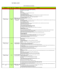
![[incr tsdb()]](http://vs1.manualzilla.com/store/data/005780303_1-7064634619abc733efac654e2a82e90d-150x150.png)