1
FFI-rapport 2014/01616
VoluViz3.1 theory and user guide – a flexible
volume visualization framework for 4D data analysis
Anders Helgeland
FFI
Forsvarets
forskningsinstitutt
Norwegian Defence Research Establishment
FFI-rapport 2014/01616
VoluViz3.1 Theory and User Guide – a Flexible Volume
Visualization Framework for 4D Data Analysis
Anders Helgeland
Norwegian Defence Research Establishment (FFI)
18 March 2015
FFI-rapport 2014/01616
1311
P: ISBN 978-82-464-2504-7
E: ISBN 978-82-464-2405-4
Keywords
Visualisering
Dataanalyse
Programmering
Approved by
Bjørn Anders P. Reif
Project Manager
Janet Blatny
Director
2
FFI-rapport 2014/01616
English summary
The key goal in scientific visualization is to transform numerical data into a visual form that enables
us to reveal important information about the data. It is a tool that engages the human senses and an
effective medium for communicating complex information. The engineering and scientific communities early employed applications of visualization. The computers were used as a tool to simulate
physical processes such as fluid flows, ballistic trajectories and structural mechanics. As the size
of the computer simulations increased, the large amount of data made it necessary to transform the
numbers from calculations into images. The use of images to communicate information is especially effective as the human visual system is able to extract an enormous amount of information
from a single image in very short time.
New challenges in scientific visualization emerge as advances in modern supercomputers make it
possible to compute bigger simulations of physical phenomena with higher precision and increasing
complexity. Contrary to the early computer simulations, current simulations often involve three
spatial dimensions in addition to time (which together result in 4D data), producing terabytes of
data containing complex dynamical and kinematical information. There are no indications that the
trend of increasing complexity in computer simulations will cease. Increased ability to model more
complex systems is an important progress, but the enormous size of present (and future) scientific
data sets demands more efficient and advanced visualization tools in order to analyze and interpret
the data.
VoluViz is a visualization tool developed at FFI which is capable of interactive visualization of large
time-dependent volumetric data. It addresses many of the challenges for large-scale data analysis
and supports a set of visualization tools to facilitate scientists in their work with huge data sets,
including effective rendering techniques, easy navigation of the data (both in time and space) as well
as advanced multi-field visualization techniques and feature enhancement techniques. The software
takes advantage of commonly available modern graphics hardware and is designed with the goal
of real-time investigation of the data. VoluViz has been used to investigate data from a number
of applications: dispersion modeling (pollution, toxic gases), biomedical flow modeling (blood
vessels, the human heart) and in industrial design optimization (aircrafts, missile seeker technology).
Choosing the right visualization can turn gigabytes of numbers into easily comprehensible images
and animations. If used properly, VoluViz can thus be an effective medium for communicating
complex information and for presenting the result from scientific simulations in an intelligible and
intuitive way, both to fellow scientists as well as a broader audience.
The report is divided into three main parts. The first part (sections 1-3) gives an overview of the
rendering framework of VoluViz in addition to the description of some important volume visualization concepts. The second part (section 4) provides a more detailed description of the rendering
algorithm used by VoluViz in addition to a presentation of the available tools with examples. The
third part (sections 5-6) provides the user manual.
FFI-rapport 2014/01616
3
Sammendrag
Formålet med vitenskapelig visualisering er å forvandle numeriske data til en visuell form som
gjør oss i stand til å vise viktig informasjon om dataene. Det er et verktøy som utnytter de menneskelige sansene og et effektivt medium for å kommunisere kompleks informasjon. Vitenskapelige
miljøer tok tidlig i bruk dette verktøyet. Datamaskiner ble brukt til å simulere fysiske prosesser som
strømninger, ballistiske baner og konstruksjonsmekanikk. Etter hvert ble datamengden så stor at det
ble nødvendig å overføre beregningstallene til bilder. Bruk av bilder er spesielt effektivt ettersom
det visuelle systemet hos mennesker er i stand til å trekke ut enorme mengder informasjon fra ett
enkelt bilde i løpet av svært kort tid.
Nye utfordringer i vitenskapelig visualisering har oppst ått parallelt med utviklingen av moderne
superdatamaskiner. Dagens maskiner gjør det mulig å beregne større og større simuleringer av
fysiske fenomener med høyere presisjon og med økende kompleksitet. I motsetning til tidligere,
inneholder dagens simuleringer ofte tre romlige dimensjoner i tillegg til tid (som til sammen fører
til 4D-data). Disse simuleringene kan produsere terabyte med kompleks datainformasjon. Det er
ingen indikasjoner på at trenden med økende kompleksitet i datasimuleringer vil stoppe. Økt evne
til å modellere komplekse systemer er et viktig framskritt, men samtidig fører størrelsen på dagens
vitenskapelige datasett til et stadig større behov for mer effektive og avanserte visualiseringsverktøy.
Visualiseringsverktøyet VoluViz er utviklet ved FFI og i stand til interaktiv visualisering av store
tidsavhengige volumetriske data. Det løser mange av de utfordringene som finnes for storskala dataanalyse og støtter et sett med visualiseringsverktøy for å hjelpe forskere i arbeidet med store datasett,
inkludert avanserte flerfeltsvisualiseringsteknikker og enkel navigering av data (både i tid og rom).
Programvaren utnytter moderne grafikkmaskinvareteknologi og er utformet med et mål om etterforskning av data i sanntid. VoluViz har blitt brukt til å undersøke data fra en rekke applikasjoner:
spredningsmodellering (forurensning, giftige gasser), biomedisinsk strømningsmodellering (blodkar, menneskehjerte) og i industriell designoptimalisering (fly, missilsøkerteknologi). Å velge riktig
visualisering kan forvandle gigabyte med tall til lett forståelige bilder og animasjoner. Brukt på
riktig måte kan VoluViz være et effektivt medium for å kommunisere kompleks informasjon og
et viktig verktøy for å presentere forskningsresultater p å en forståelig og intuitiv måte, både til
forskerkollegaer og et større publikum.
Rapporten er delt i tre hoveddeler. Den første delen (kapittel 1-3) gir en oversikt over rammeverket
i VoluViz i tillegg til en beskrivelse av noen viktige begreper i volumvisualisering. Den andre
delen (kapittel 4) gir en mer detaljert innføring i hvordan VoluViz visualiserer data, i tillegg til
en beskrivelse av tilgjengelige verktøy med eksempler. Den tredje delen (kapittel 5-6) presenterer
bruksanvisningen.
4
FFI-rapport 2014/01616
Contents
Preface
7
1
Introduction
11
2
VoluViz3.0 Framework Overview
13
3
Introduction to Volume Rendering
14
3.1
Transparency, Opacity and Alpha Values
14
3.2
Color Mapping
15
3.3
Texture Mapping
15
3.4
Direct Volume Rendering
17
3.5
Texture-Based Direct Volume Rendering
19
4
The VoluViz Rendering framework
21
4.1
Introduction
21
4.2
Flexible Direct Volume Rendering
21
4.3
Framework Overview
22
4.4
Volume Shader Scene Graph
23
4.5
Shader Code Generation
25
4.6
VoluViz Operators
26
4.6.1
Compositing Operators
26
4.6.2
Feature Enhancement Operators
30
4.6.3
Numerical Operators
35
4.7
4D Data Analysis
36
4.7.1
Animation
36
4.7.2
Time-Varying Multi-Field Volume Visualization
37
4.8
Interactive Analysis
39
5
VoluViz User Manual: Part 1 - Rendering Volumes
41
5.1
Introduction
41
5.2
Starting a VoluViz Session
41
5.3
Render Window
42
5.3.1
Using the Mouse
43
5.3.2
Light source
43
5.3.3
File Menu
43
5.3.4
Edit Menu
44
5.3.5
View Menu
46
FFI-rapport 2014/01616
5
5.4
Scene Graph Window
47
5.4.1
Using the Mouse
47
5.4.2
Item Menu
47
5.4.3
Scene Graph Rendering Area
48
5.4.4
Color Table Editor
49
5.5
Tools Window
51
5.6
Dataset Window
51
5.6.1
Data set Menu
52
5.7
Animation Window
53
6
VoluViz User Manual: Part 2 - Rendering Geometries
56
6.1
Introduction
56
6.2
Loading and rendering mesh files
56
6.2.1
Datasets Window
56
6.2.2
Vis Objects Window
57
6.3
Mesh Editor
58
6.3.1
Surface Modes
60
6.4
Setting the Light source
64
Bibliography
68
6
FFI-rapport 2014/01616
Preface
The development of VoluViz was started, in 2001, by Anders Helgeland who is the main architect
behind the software. The software has been upgraded several times in the period from 2001 to 2014,
partly with the help from some master and summer students associated with the Norwegian Defence
Research Establishment (FFI). A special thanks goes to Trond Gaarder, Geir Kokkvoll Engdahl and
Kim Kalland for their contributions. Thanks also goes to the students and scientists working at FFI,
using VoluViz, for interesting and useful discussions on how to upgrade and to further improve the
software. This also applies to all the people providing data sets used in this report.
What VoluViz is and isn’t
VoluViz was developed to overcome new challenges emerging in scientific visualization of largescale data from numerical simulations. It is designed as a Ferrari to give interactive rendering of
large time-dependent volumetric data. A high degree of interactivity is crucial to ensure an effective investigation of the data. If the visualization is carried out too slowly, we will forget what was
displayed before the next image is rendered and then lose track of the information. As a result, all
components of VoluViz (from color mapping to advanced multi-field rendering) is designed with
the goal of immediate response when investigating data.
VoluViz is, however, not designed to replace other existing visualization software. It features tools
and techniques that the other software lacks - in particular volume visualization techniques. We
have not made efforts to re-implement the parts of other software that already works sufficiently for
data visualization. VoluViz should therefore be used as one of many fine options for data investigation and data analysis. For data navigation and presentation of 3D (scalar, vector and tensor) field
components, VoluViz comes with a particularly well developed tool box.
”Have fun :)”
A caution when analyzing data
It is important to remember that the quality of the physical interpretation made when using visualization tools, in general, are no better than the quality of the original data set.
FFI-rapport 2014/01616
7
8
FFI-rapport 2014/01616
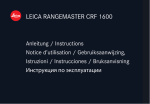
Top: Advanced focus+context visualization with the purpose of revealing and emphasizing major
arteries, known as the Circle of Willis, inside an MRI data set of a human brain (see figure 4.9).
Middle: Advanced temporal-spatial visualization of a breakdown of a single vortex ring by projecting data from six different time steps into the same scene (see figure 4.14).
Bottom: Visualization of a surface model of an industrial environment together with consentration
data (of pollution) released from the industrial plant (see figure 6.11).
FFI-rapport 2014/01616
9
10
FFI-rapport 2014/01616
(a)
(b)
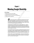
Figure 1.1 (a) Concentration of pollution released from an industrial plant [11]. (b) Visualization
of the velocity field around a carrier pod for F-16 [12]. Both visualizations were made
using VoluViz.
1
Introduction
VoluViz is a volume rendering application designed for viewing time-dependent and time-independent
(static) volumetric data. Such data is the output of a number of applications such as in dispersion
modeling (e.g. smoke, pollution), biomedical flow modeling (e.g. blood vessels, drug delivery
systems) and in industrial design optimization (e.g aircrafts, engines), see figure 1.1.
VoluViz was developed to overcome new challenges emerging in scientific visualization of large
three-dimensional (and time-dependent) data. Large tree-dimensional data sets is challenging to
visualize effectively mainly due to two reasons. Firstly, while one- and two-dimensional data sets
are rather straightforward to visualize, volumetric data sets cannot be projected to a 2D screen
without losing information. For instance, important information embedded in the data might get
lost if it is hidden behind other parts of the data or if the “wrong” parts of the domain are selected
for display. Good tools for exploring and navigating volumetric data sets, to help scientists and
engineers to convey only the important and interesting parts of the data, are therefore needed to
ensure an effective visualization. Secondly, these tools need to be interactive. A high degree of
interactivity is important when investigating data due to the short-term memory of the human brain.
If the visualization is carried out too slowly, we will forget what was displayed before the next image
is rendered and then lose track of the information.
VoluViz takes advantage of commonly available modern graphics hardware and advanced visualization techniques to implement a wide variety of visualization modes. It features tools to facilitate
scientists in their work with huge data sets including effective rendering techniques, easy navigation
of the data (both in time and space) as well as advanced multi-field visualization techniques and
feature enhancement techniques. The software is implemented in C++ [38], Qt [2], OpenGL [35]
and OpenGL Shading Language (GLSL) [32]. The development of VoluViz was initially started in
2001 by Anders Helgeland and has been upgraded several times in the period from 2001 to 2014.
FFI-rapport 2014/01616
11
It is an ongoing project, and VoluViz is still being extended to include new features to support
scientists working at the Norwegian Defence Research Establishment with data analysis and data
presentations. Choosing the right visualization can turn gigabytes of numbers into easily comprehendable images and animations. If used properly, VoluViz can thus be an effective medium for
communicating complex information and for presenting the result from scientific simulations, both
to co-workers as well as a broader audience, in an understandable and intuitive way.
The document works both as a user guide and a detailed theoretical description of some of the
visualization techniques used by VoluViz. The report is divided into tree main parts. The first part
(sections 2 and 3) provides an overview of the rendering framework of VoluViz in addition to the
description of some concepts important in volume visualization. The second part (section 4) gives a
more detailed description of the rendering algorithm used by VoluViz in addition to a presentation
of the available tools with examples. The third part (sections 5-6) provides the user manual. The
three different parts are, to some extent, independent of each other. This means that a reader could
start reading the user manual first and then move on to the other parts to learn more about details of
the software and the visualization techniques.
12
FFI-rapport 2014/01616
(a)
(b)
(c)
Figure 2.1 (a) Render window. (b) Volume Scene Graph window. (c) A transfer function editor.
2
VoluViz3.0 Framework Overview
VoluViz is a volume visualization application capable of fast visualization of 3D data defined on a
regular structured grid. As most of the rendering code is executed on the GPU (graphics processing
unit), it manages interactive analysis of quite large data. It reads files in the HDF5 [1] format and
includes a browser for easy navigation of HDF5 files. In addition, VoluViz has the following key
features:
• Fully interactive color table editor for specifying transfer functions
• Support for interactive visualization of time-varying fields
• Support for interactive multi-field visualization with custom GLSL shaders
• Interactive clip plane and picking of subset utilities for easy navigation of the data
The framework basically consists of volume data, operators to manipulate the data, a volume scene
graph, and a renderer. Figure 2.1 shows a very simple setup where a single dataset (the velocity
magnitude of a hurricane simulation [28]) is visualized using volume rendering. In this setup, the
volume data is first mapped to a color and transparency value before it is rendered in the main
VoluViz render window (figure 2.1(a)). The scene graph window can be seen in figure 2.1(b). Here,
different types of visualizations can be constructed by connecting the volume data to different types
of operators. In the current visualization, a single operator is used, namely a lookup table (LUT),
which maps every data value inside the data domain into to a color and transparency value by using
a color table editor. The lookup table (also known as a transfer function) used for constructing the
current scene can be seen in figure 2.1(c). In this case, it maps all data to grayscale values giving
maximum and minimum data values the colors white and black, respectively.
FFI-rapport 2014/01616
13
Figure 3.1 The skull of a head is emphasized by assigning low opacity to the soft tissues.
3 Introduction to Volume Rendering
Volume rendering is the process used to create images from volumetric data. Large data sets obtained from instruments (such as medical scanners) or numerical simulations have led to an increasing demand for more efficient visualization techniques. As a result, several volume rendering
techniques have emerged. As VoluViz uses a technique known as direct volume rendering as its
main rendering algorithm, this section will cover a few concepts that are important in volume visualization. Understanding these concepts will make it easier for scientists to benefit from using
VoluViz as an interactive tool for data navigation and data analysis. A more detailed and complete
description of volume visualization can be found, for instance, in [15, 42, 14].
3.1 Transparency, Opacity and Alpha Values
An important concept in visualization of volumetric data is transparency or opacity. Although many
visualization techniques involve rendering of opaque objects, there are applications that can benefit
from the ability to render semitransparent objects and even objects that emit light. The internal data
from an MRI scan can for instance be shown by making the skin semitransparent, see figure 3.1.
Opacity and transparency are complements in the sense that high opacity implies low transparency,
and are often referred to as alpha in computer graphics. The opacity or alpha value, A, is a normalized quantity in the range [0, 1]. If an object has maximum opacity (A = 1), it is opaque and the
objects and light behind are shielded and invisible. If A < 1, the object is transparent and makes
objects behind visible. An alpha value of zero (A = 0) represents a completely transparent object.
The relation between opacity and transparency, T, is given by A = 1 − T .
14
FFI-rapport 2014/01616
s i < min, i = 0
s i > max, i = n−1
i = n(
si
rgb0
rgb1
rgb2
color
s i − min )
max − min
rgbn−1
Figure 3.2 Mapping scalars to colors via a lookup table.
3.2 Color Mapping
Color mapping is a common scalar visualization technique that maps scalar data into color values
to be rendered. In color mapping, the scalar values are divided into n equal intervals and serve as
indices into a lookup table. The table holds an array of colors and is associated with a minimum and
maximum scalar data range (min, max) into which the scalar values are mapped. Scalar values with
either lower or greater value than the chosen data range is clamped to the minimum and maximum
color value, respectively. The rest of the scalar values, si , are given colors associated with the index,
i, in the lookup table, see figure 3.2.
The lookup table holds an array of colors that can be represented for example by the RGBA (red,
green, blue, alpha) or the HSVA (hue, saturation, value, alpha) color system. The RGBA system
describes colors based on their red, green, blue and alpha intensities and is used in the raster graphics
system. The HSVA system, which is by scientists found to give good control over colors in scientific
visualizations, represents colors based on hue, saturation, value and alpha. In this system, the hue
component refers to the wavelength which enables us to distinguish one color from another. The
value V which also is known as the intensity component, represents how much light is in the color
and saturation indicates how much of the hue is mixed into the color.
Use of colors is important in visualization and should be used to emphasize various features of the
data set. However, making an appropriate color table that communicates relevant information is a
rather challenging task. “Wrong use” of colors may exaggerate unimportant details. Some pieces
of advice in making appropriate color tables are given in [37, 4]. In volume visualization, lookup
tables are often referred to as transfer functions. Figure 3.3 illustrates the use of transfer functions
on data from a simulation of aerosol dispersion in an industrial environment [11].
3.3 Texture Mapping
In computer graphics, geometric objects are represented by polygonal primitives (consisting of vertices and cells). In order to render a complex scene, millions of vertices have to be used to capture
the details. A technique that adds detail to a scene without requiring explicit modeling of the detail
with polygons, is texture mapping. Texture mapping maps or pastes an image (a texture) to the
surface of an object in the scene. The image is called a texture map and its individual elements are
called texels. Texture maps can be one-, two- and three-dimensional. A texture may contain from
FFI-rapport 2014/01616
15
(a)
(b)
(c)
(d)
Figure 3.3 Visualization of concentration of pollution released from an industrial plant using the
HSVA color system for the color mapping. The consentration data are first mapped to a
voxel set with 8-bit precision (in the range [0, 255]), and serve as indices into a lookup
table giving each value a separate color and opacity value. Figures (a) and (c) show two
scenes rendered using the transfer functions displayed in (b) and (d), respectively. In both
transfer function editors, the consentration data are mapped to identical colors using
identical mappings for the HSV components. The only difference between the two scenes
is in the mapping to the opacity values also known as the alpha (A) component. While one
of the scenes is rendered with maximum opacity (A=1) for all data points, the other scene
(c) is rendered using much lower opacities resulting in a very different representation of
the data. Here, all data points containing the lowest amount of consentration are made
completely invisible (by setting alpha to zero for all these values). In addition, the rest
of the data are rendered in a semi-transparent fashion using low opacity values. A clip
plane is used in both scenes, removing all data between the clip plane and the view.
16
FFI-rapport 2014/01616
Figure 3.4 Texture mapping example in 3D. Here, a single planar surface has been cut through the
volume. Local texture coordinates are then sampled along the surface which gives the
mapping to the 3D texture storing the volumetric data. The data is then mapped to colors
and opacities and finally pasted as an image on top of the surface.
one to four components. A texture with one component contains only the intensity value, and is
often referred to as an intensity map or a luminance texture. Two component textures contain information about the intensity value and the alpha value. Three component textures contain RGB values
and a texture with four components contains RGBA values. To determine how to map the texture
onto the polygons, each vertex has an associated texture coordinate. The texture coordinate maps
the vertex into the texture map. The texture map in 1D, 2D and 3D can be defined at the coordinates
(u), (u, v) and (u, v, w), respectively, where u, v, w are in the range [0, 1].
Texture mapping is a hardware dependent feature and is designed to display complex scenes at real
time rates. While 2D textures is most common in computer gaming, both 1D and 3D textures are
widely used in scientific visualization, especially in volume rendering. One-dimensional textures
can for instance be used to store transfer functions (see section 3.2). As an example, the transfer
functions displayed in figure 3.3 are implemented using one-dimensional textures to store the data
mapping to the color and opacity components used in the visualization. Three-dimensional textures
can, for instance, be used to store volumetric scalar data fields. In volume rendering, the scalar
values are often normalized and represented as a regular structured data set with 8-bit (or 16-bit)
precision. These values can be used as indices into a lookup table. In that case, texel values in the
volume texture are mapped to color (and opacity) values to be rendered. If the transfer functions
are implemented in texture hardware, this allows an instant update of the color and opacity in the
scene after altering the lookup table. If the transfer functions are not supported in hardware, the 3D
textures have to be regenerated every time the lookup table changes. Figure 3.4 illustrates the use
of texture mapping, where concentration data (of pollution) from an industrial plant is mapped to
colors and then pasted as an image onto a single surface intersecting the data domain.
3.4 Direct Volume Rendering
Direct volume rendering is a group of rendering methods that generates images of volumetric data
sets without explicitly extracting geometric surfaces from the data. In direct volume rendering,
FFI-rapport 2014/01616
17
voxels are used as building blocks to represent the entire volume. Typically, each voxel is associated
with a single data point which is mapped to optical properties such as color and opacity (see figure
3.5(b)). As opposed to the indirect techniques, such as isosurface extraction [24, 27, 34], the direct
methods immediately display the voxel data. These methods try to give a visual impression of
the complete 3D data set using light transport models which describes the propagation of light in
materials. During rendering, the optical properties are accumulated along each viewing ray to form
an image of the data (see figure 3.5(a)). An overview of different optical models ranging from very
simple to very complex models that account for absorption, emission as well as scattering effects
can be found in the work by Max [26]. The most widely used method for volume rendering is the
one limited to absorption and emission effects only. This emission-absorption [26] model can be
expressed by the differential equation
dIλ
= gλ (s) − τ (s)Iλ (s),
(3.1)
ds
where Iλ (s) = Iλ (x(s)) is the intensity of radiation with wavelength λ at the position s along
the ray x(s). The function gλ (s) = Cλ (s)τ (s) is called the source term and describes the emissive
characteristics throughout the volume. Here, Cλ (s) is the emissive color contribution at a point x(s)
in the volume. The function τ (s) is called the extinction function and gives the amount of radiation
that is absorbed. Solving equation (3.1) by integrating from s = 0 at the edge of the volume to the
endpoint s = D leads to the volume rendering integral (VRI)
Iλ (D) = Iλ (0)e−
RD
0
τ (t)dt
+
D
Z
Cλ (s)τ (s)e−
RD
s
τ (t)dt
ds.
(3.2)
0
The term Iλ (0) gives the light coming from the background at the position s = 0 and Iλ (D) is
the total intensity of radiation leaving the volume at s = D and finally reaching the eye. The first
term represents the light from the background multiplied by the volume’s transparency between
s = 0 and s = D. The second term represents the integral contribution of the source term at each
position s, multiplied by the volume’s transparency
R along the remaining distance to the eye. Using
− ss2 τ (t)dt
this definition of the transparency, T (s1 , s2 ) = e 1
, we obtain a slightly different version of
the volume rendering integral
Iλ (D) = Iλ (0)T (0, D) +
Z
D
Cλ (s)τ (s)T (s, D)ds.
0
By approximating the VRI (3.2) with a Riemann sum and using a second order Taylor series to
approximate the exponential, we get the discrete volume rendering integral (DVRI)
L/∆s−1
Iλ (D) =
X
L/∆s−1
Cλ (i∆s)A(i∆s)
i=0
Y
(1 − A(j∆s)),
j=i+1
(3.3)
with gλ (0) = Cλ (0)A(0) = Iλ (0).
Here, A(i∆s) = (1 − T (i∆s)) ≈ (1 − (1 − τ (i∆s)∆s)) = τ (i∆s)∆s is the opacity. When
looking at equation (3.3), the reason for preferring this particular discretization of the VRI becomes
18
FFI-rapport 2014/01616
(a)
(b)
Figure 3.5 (a) In Ray Casting, the final image is obtained by sending rays from the screen into the
scene. The final color at each pixel is obtained by evaluating a rendering integral along
samples containing optical properties (color and opacity) along each ray. (b) Data to be
rendered are typically represented as a voxel set. Each voxel is associated with a single
data point which is mapped to a color and opacity value giving the local emissive and
absorption properties which can be used directly in the emission-absorption [26] model.
apparent. It is equal to the recursive evaluation of the over operator [30]. Not only is this a useful
theoretical tool for describing the science behind direct volume rendering, but it also enables the use
of existing general compositing (software and hardware) algorithms to render volumes.
In order to produce images of the volume data, an algorithm must be used to evaluate the volume
rendering integral (equation (3.3)). The conceptually most simple algorithm is ray casting [9, 22],
since it immediately follows from the discussion above. The basic idea of ray casting is to determine
the value of each pixel in the image by sending a ray through the pixel into the scene. Typically,
when rendering volumetric data, the rays are parallel to each other and perpendicular to the view
plane, see figure 3.5. The DVRI (equation (3.3)) is then evaluated for each ray by sampling the
volume at a series of sample points a distance ∆s apart.
Other direct volume rendering techniques are splatting [44], shear-warp [21], and texture-based
direct volume rendering [7, 8], which is the algorithm VoluViz is based upon.
3.5 Texture-Based Direct Volume Rendering
Hardware assisted volume rendering using 3D textures can provide interactive visualizations of 3D
scalar fields [7, 8], The basic idea of the 3D texture mapping approach is to use the scalar field
as a 3D texture. If the texture memory is large enough, the entire volume is downloaded into
the texture memory once as a preprocess. To render the voxel set, a set of equally spaced planes
(slices) parallel to the image plane are clipped against the volume. The hardware is then exploited
FFI-rapport 2014/01616
19
Voxel set
Data
Transfer function
Texture
memory
Volume slicing
Figure 3.6 Direct volume rendering by texture slicing. First, data volumes and color tables are
uploaded to texture memory on the graphics card as a preprocess. Then, a set of view
aligned slices are clipped against the volume and blended in a back-to-front order. The
bottom left image shows the result from applying volume slicing on a data set using four
slices only. In the bottom right image, a considerably larger amount of planes are used
to render the same data set. This gives a much more continuous visualization of the data.
to interpolate 3D texture coordinates at the polygon vertices and to reconstruct the texture samples
by trilinearly interpolating within the volume. If a transfer function is used, the interpolated data
values are passed through a lookup table that maps the values into color and opacity values. This
way, graphics hardware allows fast response when modifying color and opacity. Finally, the volume
is displayed by blending the texture polygons back-to-front onto the viewing plane using the over
operator [30] (which is equivalent to solving equation (3.3)). This technique is called texture slicing
or volume slicing. Texture slicing is capable of producing images of high quality at interactive rates.
Figure 3.6 shows an illustration of the steps involved when rendering volumes using texture-based
direct volume rendering.
Although 3D texture mapping is a powerful method, it strongly depends on the capabilities of the
underlying hardware. When the size of the volume data sets exceeds the amount of available texture
memory, the data can be split into subvolumes (or bricks) that are small enough to fit into memory.
Each brick is then rendered separately, but since the bricks have to be reloaded for every frame, the
rendering performance decreases considerably.
20
FFI-rapport 2014/01616
4
The VoluViz Rendering framework
4.1 Introduction
Even though most computer simulations involve the solution of a multiple set of related data fields,
much of the current data analysis focus on studying the data in a single-field variable manner only.
While single-variable visualizations can satisfy the needs of the user in many applications, it is clear
that in some areas, such as in fluid mechanics research, it would be extremely useful to be able to
effectively visualize multiple fields simultaneously and the relation between them. However, due to
perceptual issues, such as clutter and occlusion, it can be very challenging to produce an effective
visualization of multiple volumetrical fields.
To facilitate a more effective visualization of multiple data fields, VoluViz is designed using a flexible multi-field visualization framework that is capable of combining a multiple set of data fields
(both temporal and spatial) into a single field, for rendering. This is achieved through a set of operators. The final output is selected through a powerful and flexible graphical user interface which
makes it very easy to change between different types of visualizations. The user interface allows
the generation of visualization scenes through drag and drop events, connecting the operators into
a volume scene graph. To enable interactive analysis, each visualization scene, which is the outcome of a tree graph, is converted to a mathematical expression and corresponding GPU (graphics
processing unit) shader code to be run on the graphics card.
Interesting features in the data can be emphasized by manipulating transfer functions (to control
color and transparency of the data) in addition to applying feature enhancement techniques to enhance depth, boundaries, edges, and detail. The latter techniques can be used to give the user a
better appreciation of the three-dimensional structures in the data.
4.2 Flexible Direct Volume Rendering
Our rendering framework is based on texture-based direct volume rendering [7, 8] which is explained, in detail, in section 3.5. Here, a set of view aligned slices are clipped against the volume
and blended in a back-to-front order. The hardware is then exploited to interpolate 3D texture coordinates at the polygon vertices and to reconstruct the texture samples by trilinearly interpolating
within the volume. Typically, for single-field data volume rendering, data values are sampled at
each sample position on the view-aligned slice planes. The data values are then mapped to a color
and transparency value and then used directly in the (discrete) volume rendering integral
L/∆s−1
Ieye =
X
L/∆s−1
C(i∆s)A(i∆s)
i=0
Y
(1 − A(j∆s)).
(4.1)
j=i+1
This particular integral is derived from the emission-absorption [26] model where C(i∆s) and
A(i∆s) are the emissive color and opacity contribution at given sample points in the volume and
∆s is the sampling distance between the individual slice planes.
VoluViz however, takes advantage of the flexibility of modern graphics hardware to implement a
much more flexible variant of volume rendering. On modern graphics hardware, a separate program,
FFI-rapport 2014/01616
21
Voxel sets
A
Data
B
Texture
memory
Transfer functions
Volume slicing
Color = ?
A
B
Opacity = ?
A merge B
Figure 4.1 Flexible volume rendering pipeline used by VoluViz. By writing separate GPU programs
called shaders, allows the user to control what is sent as local color and opacity values
when evaluating the volume rendering integral (eq. 4.1). Hence, it is possible implementing compositing operators, such as the merge operator, for local blending of multiple
data sets.
referred to as a fragment program, or a fragment shader, can be called for each time a single volume
sample is processed in the above volume integral. This means that we can override what is sent
as color and opacity contributions, and write our own shaders. This enables a flexible way of
implementing a number of more sophisticated volume rendering techniques such as volume shading,
non-photorealistic volume rendering techniques as well as multi-field volume rendering.
A sketch of the flexible volume rendering pipeline can be seen in figure 4.1. As opposed to traditional volume rendering, which only handles a single data set, VoluViz can visualize data from
a multiple set of data fields simultaneously. This means that we can upload multiple data sets and
their associated transfer function into texture memory on the graphics card and then control the local
output by our fragment program. This is illustrated in the bottom right image of figure 4.1, where
the two data sets A and B are merged locally into the same scene using a merge operator.
4.3 Framework Overview
To benefit from the flexible volume rendering pipeline, a powerful and intuitive framework is needed
that allows the user to quickly change between different data sets and types of visualization techniques.
The framework basically consists of data objects, volume objects, a volume scene graph, and a
renderer. First, the selected data fields are stored as data objects together with information such as
22
FFI-rapport 2014/01616
(a)
(b)
Figure 4.2 (a) Volume shader scene graph. (b) Four different shader items and their connection
areas. Single field areas are drawn as straight rectangles while multiple field areas are
drawn as rounded rectangles.
data range and time information. Then, volume objects are created from the data sets and put in
the volume scene graph. Each volume object is defined by a uniform 3D scalar field and stored as
a separate 3D texture on the graphics card. In this process, the original data values are normalized
and stored according to the internal texture format specified by the user. The framework supports
8-bit, 16-bit as well as 32-bit (floating point) precision.
A visualization scene graph is then created by connecting the volume objects to supported operators
through a flexible graphical user interface (GUI). The scene graph is then automatically converted
to a shader program which is used in the volume rendering pipeline.
4.4 Volume Shader Scene Graph
The scene graph consists of a set of nodes, called shader items or scene graph items, with input
areas on the top and output areas on the bottom (see figure 4.2). The shader items are connected by
connecting the input and output areas through drag and drop events.
To increase the user friendliness, the color and opacity (represented by the red, green, blue, and
alpha, (r,g,b,a), components), which are the output of most of the shader items, are hidden from
the user. This simplifies the GUI and makes it easier to switch between different visualization
scenes. For single-value operators 1 such as the diff operator, which can be used to calculate the
local difference between two selected data sets, the input values are transferred through the alpha
1
While many of the shader items have the four (r,g,b,a) components as inputs, single-value operators only need a
single component as input which is sent through to the shader item as the alpha component.
FFI-rapport 2014/01616
23
component. For consistency, the resulting output value is copied to all the (r,g,b,a) components.
The same applies for the volume node which copies the sampled (scalar) data volume values, after
texture lookup, in a similar way. The connection (input and output) areas of the shader items are
currently of the two types RGBA and Gradient. They can either be defined as a single-field or a
multi-field connection area. While single-field areas only support a single connection to any other
shader item, multi-field areas can be connected to a multiple set of nodes. Single-field areas are
drawn as straight rectangles whereas multi-field areas are drawn as rounded rectangles (see figure
4.2(b)).
The shader scene graph consist of a number of various shader items and is continuously extended
to include new operators. Currently, the following shader items are supported:
• Volume: Returns data values from the associated data set after a 3D texture lookup.
• LUT: Performs a 1D transfer function lookup. A lookup table (LUT) can be used at any level
in the scene graph. More details on transfer functions can be found in section 3.2 which
covers color mapping. A graphical user interface of the transfer function editor is obtained by
double-clicking on the shader item. More details on how to use the transfer function editor
can be found in section 5.4.4.
• Color Out: This is the root node of the shader graph. It contains the final (C, A) = (RGB, A)
values that are used in the volume rendering integral (eq. 4.1).
• Compositing Operators: The scene graph supports all the compositing operators defined by
Porter and Duff [30] and the merge operator defined by Helgeland et. al. [17].
• Color/Alpha: Combines two fields by taking the RGB values from the first field and the
opacity value from the second field.
• Mask: This operator combines two fields by multiplying the alpha value of the first chosen
field with the alpha value of the second field, while taking the RGB value from the first field.
• Diff: Computes the difference between two fields.
• AbsDiff: Computes the absolute difference between two fields.
• Gradient: Computes the gradient using a second-order central difference scheme. The evaluated gradient is based on the total expression that is sent as input to the gradient operator.
• NormalizeGrad: Can be used to visualize the gradient field. It normalizes the local gradient
and sends the vector component values through the RGB values. The alpha value is set to 1.
• GradientCorr: Evaluates the gradient similarity measure [33] of two selected fields.
• Lighting: Computes the Blinn-Phong [6] volume shading model.
• Contours: Computes contours from the the input field. This operator can be used to create
silhouettes.
24
FFI-rapport 2014/01616
4.5 Shader Code Generation
Our shader composer evaluates the volume shader expression through a recursive traversal of the
shader tree graph starting from the Color Out root node. First, all the volumes and LUTs are located. Once found, the corresponding data objects are located and converted to 3D and 1D textures,
respectively. A shader program is then generated by replacing all of the shader nodes with corresponding GLSL shader language code. A new shader program is created every time the user makes
changes to the scene graph. For instance, the shader graph depicted in figure 4.2(a) is converted to
the following shader code.
/ ∗ S h a d e r g e n e r a t e d by VoluViz ∗ /
uniform
uniform
uniform
uniform
varying
s a m p l e r3 D Volume1 ;
s a m p l e r3 D Volume2 ;
s a m p l e r1 D LUT1 ;
s a m p l e r1 D LUT2 ;
v e c 3 TexCoord0 ;
v o i d main ( )
{
/ ∗ Res1 = Volume1 ∗ /
v e c 4 Res1 = t e x t u r e 3 D ( Volume1 , TexCoord0 . xyz ) . r g b r ;
/ ∗ Res2 = LUT1 ( Res1 ) ∗ /
v e c 4 Res2 ;
Res2 . r g b = t e x t u r e 1 D ( LUT1 , Res1 . r ) . r g b ;
Res2 . a = t e x t u r e 1 D ( LUT1 , Res1 . a ) . a ;
/ ∗ Res3 = Volume2 ∗ /
v e c 4 Res3 = t e x t u r e 3 D ( Volume2 , TexCoord0 . xyz ) . r g b r ;
/ ∗ Res4 = LUT2 ( Res3 ) ∗ /
v e c 4 Res4 ;
Res4 . r g b = t e x t u r e 1 D ( LUT2 , Res3 . r ) . r g b ;
Res4 . a = t e x t u r e 1 D ( LUT2 , Res3 . a ) . a ;
/ ∗ Res5 = Atop ( Res2 , Res4 ) ∗ /
v e c 4 Res5 ;
Res5 . r g b = Res2 . a ∗ Res2 . r g b + ( 1 − Res2 . a ) ∗ Res4 . r g b ;
Res5 . a = Res4 . a ;
g l F r a g C o l o r = Res5 ;
}
The most complex shader item is the gradient operator. Since the gradient can be evaluated at any
level in the scene graph this implies that the entire expression prior to the gradient node has to
be evaluated at six different sample positions (assuming a second order finite difference scheme is
used). The beauty of the system is that any new field can be computed in the scene graph, mapped
to a color and alpha value through a separate texture lookup, and then rendered correctly with a
gradient based light model or a non-photorealistic rendering technique.
Figure 4.3 shows an example where data from a hurricane simulation [28] is rendered using a bit
more advanced scene graph construction including the computation of gradients and the use of a
gradient based light model.
FFI-rapport 2014/01616
25
Figure 4.3 Visualization of volumetric streamlines giving the local wind direction of the hurricane
data. The streamlines (volume2) are color encoded by the velocity magnitude (volume1)
using the Color/Alpha operator and rendered using a gradient-based light model.
4.6 VoluViz Operators
4.6.1 Compositing Operators
One method for combining multiple data sets into a single field is by using the compositing operators
presented by Porter and Duff [30]. Here, a composited color and opacity value of the two volumes
A and B is obtained by the formulas
A = aA FA + aB FB ,
(4.2)
cA aA FA + cB aB FB
,
(4.3)
A
where ci and ai are the color and opacity values associated with the contributing volumes and Fi
is a weight function. The following combination of weight functions defines the operators given
in table 4.1. These operators are very useful for showing correlation between multiple data fields,
such as finding overlapping regions of selected data sets. Different operators correspond to different
visible regions using union and intersection operations on the opacity values.
C=
As an additional compositing operator we have also implemented the merge operator presented by
Helgeland et. al. [17]. For some applications, the merge operator is preferable compared to, for
instance, the over operator since this expression holds no precedence in any area covered by multiple
data fields (see table 4.1). It also handles arbitrary number of input fields as opposed to the binary
operators presented by Porter and Duff. The merge operator is given by the formulas
n
Y
A = 1 − (1 − ai )
(4.4)
n
n
X
X
ai .
ci ai )/
C=(
(4.5)
i=1
i=1
i=1
26
FFI-rapport 2014/01616
Table 4.1 Compositing operators. The alpha (or opacity) values are set to be completely opaque
(ai = 1) for both the visible (blue and red) regions defined by the data sets A and B in all
the examples.
FA
FA
A
1
0
B
0
1
A over B
1
1 − aA
B over A
1 − aB
1
A in B
aB
0
B in A
0
aA
A out B
1 − aB
0
B out A
0
1 − aA
A atop B
aB
1 − aA
B atop A
1 − aB
aA
A xor B
1 − aB
1 − aA
eq. (4.4),(4.5)
eq. (4.4),(4.5)
Operations
A merge B
FFI-rapport 2014/01616
27
Result
(a)
(b)
Figure 4.4 (a) Visualization of vortices generated in the wake of a radome mounted on the P3-C
aircraft. (b) A zoomed in rendering of the vortices.
Figure 4.5 gives an example where we demonstrate the usefulness of the compositing operators
by showing relationships between three different vortex identification measures used on a channel
flow simulation data set [13]. In fluid dynamics research, the study of vortices is important for
understanding the underlying physics; vortices are often viewed as “the sinews and muscles of
turbulence” [20]. In engineering applications, vortices can either be desirable or undesirable and
attempts to promote or to prevent the occurrence of vortices are used for optimizing and modifying
design. Figure 4.4 shows an example of undesirable vortex formations created in the wake of a
radome mounted on the P-3C aircraft [5]. The turbulent wake impacts the aft part of the aircraft and
may trigger vibrations in the aircraft.
Many vortex-detection methods have been proposed in the literature. Among the most popular and
successful identifiers are the three criteria
• helicity (v · ω),
• enstrophy (kωk2 ), and
• λ2 [19],
where v and ω are the velocity and vorticity vectors, respectively.
In Figure 4.5(a), the relation between the λ2 and the enstrophy field is revealed using the atop
operator. The operation (λ2 atop enstrophy) gives a rendering where the visible region (given by
the opacity) is defined by the enstrophy field while the color is determined by both fields but with
an emphasis on the λ2 field. Setting the alpha values of the λ2 structures equal to one results in a
rendering where regions occupied by the intersection of the two fields are colored by the λ2 field
while the remaining region of the enstrophy structures is colored by the enstrophy field. Hence, we
are able to see the spatial relation between the two fields. Regions of high vorticity magnitude result
both in vortex cores and vorticity sheets. By using the atop operator we are thus able to distinguish
between the vortex cores (red) from the vorticity sheets (gray/white) as can be seen in figure 4.5(a).
28
FFI-rapport 2014/01616
(a) λ2 atop enstrophy
(b) Helicity in λ2
Figure 4.5 Visualization of relationships between three different vortex identification measures using
compositing operators. (a) The operation λ2 atop enstropy is used to distinguish the
vortex cores (red) from the vorticity sheets (gray/white). (b) Individual vortices defined
by the λ2 criterion are colored by the helicity using the in operator. Red and blue colored
vortices indicate clockwise and counter clockwise rotation, respectively.
FFI-rapport 2014/01616
29
Figure 4.5(b) gives another example where the in operator is used to convey information about the
spatial correlation between helicity and vortices defined by the λ2 criterion. Here, the visible region
is defined by the λ2 field while the color is determined by the helicity field. There is a strong
correlation between helicity and coherent structures in a turbulent flow field, and this quantity has
previously been used to extract vortex core lines [23]. The assumption is that that near vortex core
regions, the angle between v and ω is small, which means that local extreme values of helicity can
be used as indicators of vortex cores. The sign of the helicity value indicates the direction of the
rotation (or swirl) with respect to the streamwise velocity component. Positive values give clockwise
rotation while negative values give counter clockwise rotation. In figure 4.5(b) individual vortices
defined by the λ2 criterion are colored by the helicity. Red and blue vortices indicate clockwise and
counter clockwise rotation, respectively.
4.6.2 Feature Enhancement Operators
Even though the emission-absorption model [26] and the resulting volume rendering integral (equation (4.1)) does not take external light sources into account, shading of volumes can still be achieved.
Volume shading can increase realism and understanding of volume data. Most volume shading is
computed using the Phong [29] or Blinn-Phong [6] illumination models. The resulting color is a
function of the gradient, light, and view direction, as well as the ambient, diffuse, and specular
shading parameters.
Traditional local illumination models is based upon a normal vector which describes the orientation
of a surface patch. In volume rendering no explicit surfaces exist. So instead, the model is adapted
assuming light is reflected at isosurfaces inside the volume data. For a given point p an isosurface
is given as:
I(p) = {x|f (x) = f (p)}
with normal, n, defined as
n(p) =
∇f (p)
,
k∇f (p)k
∇f (x) =
∂f (x) ∂f (x) ∂f (x) .
,
,
∂x
∂y
∂z
A local illumination model can thus be incorporated into the emission-absorption model by using
the gradient, ∇f (p), as the normal vector. The volume shading is typically added to the emissive
color contribution in the emission-absorption model resulting in an alternative color contribution,
C volume , substituting the pure emissive term in the volume rendering integral (eq. 4.1) by
C volume = C emission + Cillumination ,
(Cillumination = IPhong |IBlinnPhong ).
(4.6)
The Blinn-Phong model can, for instance, be expressed as
IBlinnPhong = Iambient + Idiffuse + Ispecular ,
= ka + kd (l · n) + ks (h · n)s ,
(4.7)
where l is the light direction vector, h is the half vector which is halfway between the viewing
vector and the light direction, s is the specular power and ka , kd and ks are the ambient, diffuse and
specular coefficients.
30
FFI-rapport 2014/01616
(a)
(b)
(c)
(d)
Figure 4.6 (a) Traditional direct volume rendering without any feature enhancements with associated transfer function (b). (c) Gradient-based volume shading (Blinn-Phong model) with
associated transfer function.
Figure 4.6 demonstrates the effect of applying gradient-based volume illumination to a selection of
vortices from a simulation of stratified turbulent shear layer [43]. The figure shows the rendering
result both with and without a local illumination model, in addition to the transfer function used for
the two cases.
It is important to note that the transfer function gives the mapping to the emissive term in equation
(4.6) only and that the contribution from the illumination model is added to the emissive term to
produce the final local color. As a result, more ”white” light is added to the scene when applying
volume illumination compared to traditional volume rendering (when using the same transfer function for the emissive color). When designing transfer functions well suited for volume illumination,
a piece of advice is thus to use lower values for the Value component in the HSV color system
(see section 3.2) than what would be ideal for traditional volume rendering without a local illumi-
FFI-rapport 2014/01616
31
Figure 4.7 Visualization of contours in a volumetric teddy bear and torus data set.
nation model. This is illustrated in figure 4.6. Here, a constant Value, V = 0.65, is used for the
transfer function associated with the local illumination model, whereas V = 1 is used for the pure
emission-absorption model.
Another way of enhancing volume data features is by using Non-Photorealistic Volume Rendering
(NPVR) techniques. The overall goal of NPVR is to go beyond the means of photorealistic volume rendering and produce images that emphasize important features in the data, such as edges,
boundaries, depth, and detail, to provide the user with a better appreciation of the three-dimensional
structures in the data. NPVR techniques are able to produce artistic and illustrative effects, such
as feature halos, tone shading, depth enhancements, boundary enhancements, fading, silhouettes,
sketch lines, stipple patterns, and pen-ink drawings [18, 40, 31, 36, 25, 16]. For volumetric data, silhouettes or contours can, for instance, be obtained by computing a contour intensity field, Icontours ,
evaluated by the following equation
Icontours = g(k∇f k)(1 − k(v · nk)n .
(4.8)
In our implementation of the contours operator, the derived intensity field, Icontours defines the
opacity while the colors is sent as input parameters to the operator. Figure 4.7 shows an example
where equation (4.8) has been used to create volumetric contours of two data sets using g(k∇f k) =
k∇f k and n = 8.
Figure 4.8 illustrates different feature enhancement techniques used on a selection of vortices from a
channel flow [13]. The images clearly reveal how volume shading and non-photorealistic rendering
techniques can add detail, enhance spatial structures and give the necessary 3D appearance of the
volume data.
The above example also demonstrates the flexibility of the presented visualization framework. As
volume shading and NPVR techniques, in addition to compositing operators and transfer functions,
can be assigned individually to all of the volume data objects, this provides a detailed control of the
final rendering appearance, enabling a numerous variety of visualizations such as the ones depicted
32
FFI-rapport 2014/01616
(a)
(b)
(c)
(d)
(e)
(f)
Figure 4.8 Feature enhancement techniques used on a selection of vortices. (a) direct use of the
volume integral given in equation (4.1) without any feature enhancements. (b) Gradientbased volume shading (Blinn-Phong model). (c) Feature enhancement using limb darkening [16]. (d) Volume shading in combination with limb darkening. (e) Silhouette
rendering using the gradient-based contour operator. (f) Volume shading in combination
with silhouettes.
FFI-rapport 2014/01616
33
(a)
(b)
Figure 4.9 (a) Regular volume rendering of an MRI data set [41] of a human brain. (b) Volume
rendering (of the same data) in combination with compositing operators and feature
enhancement techniques used with the purpose to reveal (and emphasize) arteries in the
human brain.
in figure 4.9. Here, a single MRI data set of a human head [41] is visualized with different rendering
techniques resulting in two quite different visualizations. One of the visualizations is rendered with
regular volume rendering (figure 4.9(a)) while the other one is visualized using a combination of
compositing and feature enhancement operators (fig 4.9(b)). The latter visualization is generated
with the purpose of emphasizing the major bloodvessels inside the human brain revealing a ring of
arteries located at the base of the brain known as the Circle of Willis.
Figure 4.10 shows another example where non-photorealistic rendering techniques have been used
to visualize data from a hurricane simulation [28]. Here, areas with the greatest wind speed have
been rendered in grey colors using volume shading (revealing the 3D structure of the hurricane)
while areas with the lowest wind speed have been rendered in white to red colors using volumetric
contouring (revealing the eye of the hurricane).
In both the two latter examples (figure 4.9 and figure 4.10) variations of a branch of techniques
known as focus+context visualization has been used. In focus+context visualizations, some objects
or parts of the data are shown in detail, while other objects or parts act as a context. While the data
”in focus” often are displayed rather opaque (to emphasize these regions), the rest of the data can
be shown rather transparent.
34
FFI-rapport 2014/01616
Figure 4.10 Hurricane data visualized using two different rendering techniques. Areas with the
greatest wind speed are rendered densely, in gray, (with high opacity) using volume
shading to enhance the 3D structure of the hurricane. Areas with the lowest wind speed
are visualized in a more semitransparent way (using lower opacities) in combination
with silhouette rendering, in white to red colors, to reveal the eye of the hurricane.
4.6.3 Numerical Operators
In addition to the compositing and feature enhancement operators, numerical operators acting directly on the volume data can also be incorporated in the proposed visualization framework. Two
operators that we have found particularly useful are the operators Diff and AbsDiff given as
Diff(A, B) = A − B,
AbsDiff(A, B) = kA − Bk,
Diff ∈ [−1, 1],
AbsDiff ∈ [0, 1].
These can be used to estimate the local difference between two data fields. The difference operators
can be used for a variety of applications. It can for instance be used for debugging of numerical
code, but also for finding the effect of adjustments made to a simulation. These can range from
minor adjustments such as the change of simulation parameters to larger adjustments including
the change of boundary conditions and choice of model, to major adjustments such as adding or
removing terms in the mathematical equation describing the problem. In addition, it can be used
to visualize the change occurring between different time steps of a simulation such as calculating
time derivatives. Time derivatives can be obtained by calculating finite differences, which can be
computed using the diff operator on two copies of a chosen data field with a time difference equal
to one. Then, a first order backward or forward difference can be obtained depending on the setup.
Figure 4.11 gives an example where the AbsDiff operator has been used to examine the convergence
of statistical steady turbulence in a chamber simulation [11]. The visualization shows regions where
FFI-rapport 2014/01616
35
Figure 4.11 Visualization of statistically non-converged regions of a turbulent chamber flow simulation.
the statistics of the flow has not yet reached a fully converged state. This is done by computing the
root-mean-square (RMS) of the velocity for two different time steps for a given time interval. For
statistically converged regions the RMS value should not change, which means that we can visualize
numerically non-converged regions inside the computational box by applying the diff operator on
the two RMS fields and then render all areas that are not close to zero. Figure 4.11 shows the result
after a transfer function lookup table (LUT) has been connected to the output from the diff operator
in addition to a gradient-based volume shader operator.
Figure 4.12 provides another example where where the diff operator is used to compare two channel flow simulations [13] using different boundary conditions. While the first data set is obtained
using no-slip boundary conditions, the second channel flow simulation is generated by first splitting
the channel in the middle and then using a slip boundary condition at one of the surfaces. Data
derived from the second simulation is then compared to data from half of the channel from the first
simulation. The data is compared by visualizing regions of difference only. Similar to the previous
example (see figure 4.11), regions of difference are enhanced using gradient based volume shading.
Volume shading has, in both cases, been used in combination with limb darkening [16] to highlight
the boundaries of the visualized regions.
4.7 4D Data Analysis
4.7.1 Animation
Once the desired data is selected and an appropriate visualization scene is created, our visualization
framework handles two types of navigations through the time-varying data set. The data set can
be explored by either dragging a time slider or by using the animation utility. The time slider is
36
FFI-rapport 2014/01616
Figure 4.12 Comparison of two channel flow simulations with different boundary conditions by visualizing the local difference between the two solutions.
very useful for investigating the data at different time steps. Once a new time step is selected,
the visualization scene graph is automatically updated accordingly. The time slider feature also
simplifies the process of finding transfer functions that are well-suited for the whole time-series.
Finding good transfer functions is often a tedious process that sometimes involves clipping of data
value ranges. To facilitate this process we have implemented a histogram renderer that also updates
according to the time slider. The user can select between continuous update or updates that occur
only when the time slider is released.
The animation utility, on the other hand, allows a pre-defined and a more controlled animation of
the time-dependent data. Here, the user can select the time interval, the order of the data sets to be
loaded, the step size, as well as pre-generated user interactions such as rotation and zooming.
4.7.2 Time-Varying Multi-Field Volume Visualization
The most common method to investigate the time-dependent behavior of a data set is through animation. Even though animations can be sufficient, for a number of applications, it can be difficult to
analyze spatio-temporal relationships using this technique. This is due to the loss of positional information when moving between individual time steps. To facilitate a more complete spatio-temporal
investigation of the multi-variate and time-varying data, VoluViz is designed using a novel 4D data
analysis framework. Instead of just relying on animation utilities, VoluViz also support the projection of a multiple set of data fields (both temporal and spatial) in the same scene. This extended 4D
analysis functionality is incorporated into the already presented shader scene graph (section 4.4) in
the following way. Multiple copies of selected data fields from the time-varying data sets can be
generated by the user. Each of these n copies have assigned a local time difference which is added
FFI-rapport 2014/01616
37
0
+5
+10
Figure 4.13 An example of a volume scene graph used to visualize data from three different time
steps in the same scene.
to the global time to produce the local time of each copy
(time)i = global time + (time difference)i ,
i = 1...n.
(4.9)
When data copies are used to generate volume objects in the volume scene graph, the local time of
each volume is used when accessing the data. Hence, the volume scene graph can consist of multiple
data fields from different time steps. This allows the computation of time-varying quantities such
as time derivatives (provided that the time difference is sufficiently small) and high-dimensional
projection volumes. When the global time is changed, all of the data volumes in the scene graph are
adjusted accordingly. For example, if the scene graph is constructed to visualize the spatio-temporal
relationship of a time-evolving volume structure by visualizing the structure at three different time
steps (t1 = 0, t2 = 5, t3 = 10) for t = 0 together in the same scene, an animation of the scene will
preserve the time difference between the volumes for all scenes (as long as the local time steps are
inside the global time interval). Hence, we get a 4D visualization which both exhibit time-evolution
as well as the depiction of spatio-temporal relationships at each time step of the animation. Figure
4.13 gives an example of how such a scene graph can be constructed.
Figure 4.14 gives an example where the 4D data analysis framework of VoluViz has been used to
depict the spatio-temporal evolution of the breakdown of a single vortex ring. Here, the vortex
structure is rendered in the same scene (using the merge operator) at six different time steps using
a constant time step size between the time-varying data. To distinguish between the individual time
steps, the vortex structure is visualized using six different colors starting from red color (giving the
earliest time step) to a purple depiction of the vortex structure (showing the latest time step in the
time-evolution). The visualization clearly depicts how the ring structure both moves and deforms in
space as time evolves. For instance, one is able to see how the ring first increases in size, then starts
to tilt forward before it begins to break down.
38
FFI-rapport 2014/01616
Figure 4.14 Temporal-spatial visualization of a breakdown of a single vortex ring by simultaneously
rendering the data from six different time samples in the same scene (represented by six
different colors).
Another example showing the usefulness of the 4D analysis framework is the one presented in the
second paragraph of section 4.6.3 and in figure 4.11. Here, two different time steps of a derived statistical quantity is compared to reveal all statistically non-converged regions of a turbulent chamber
flow simulation.
In addition to the local time difference functionality, each individual data object can also be ‘frozen‘
in time. This functionality can for instance be used for visualizing the time-evolution of volume
structures starting from a fixed time, with the initial structure kept in the scene for all time steps.
With two fixed time steps (t1 = A and t2 = B), an animation could show how the structure evolves
from time step A to time step B, with both fixed structures kept in the scene for all frames. This
is illustrated in figure 4.15. Here, a silhouette rendering of the hurricane [28] is rendered at two
fixed time steps for all frames to provide contextual information, thus increasing the depiction of
temporal-spatial relationships in the data.
4.8 Interactive Analysis
To facilitate interactive analysis of a three-dimensional time-dependent data set, the rendering framework of VoluViz supports an additional set of tools. In addition to manipulating the volume scene
graph and individual transfer functions, the system supports clip planes manipulation, data-subset
selections, and other user functions, at interactive rates. These are all tools that can be used to diminish the occlusion effects by for instant reducing the complexity of the scene by focusing on a
region of interest.
In addition, a data caching system is implemented allowing whole time series of selected data sets
FFI-rapport 2014/01616
39
(a) t = 0
(b) t = 15
(c) t = 30
(d) t = 45
Figure 4.15 Snapshots from an animation of a hurricane data set where silhouettes of the hurricane
at two fixed time steps are rendered in all frames.
to be cached in the CPU memory, assuming there is enough memory available to fit the entire data
set. As the transfer of data from the hard-drive to CPU-memory tends to be the main bottle-neck for
the animation system, this helps speeding up animations. This caching mechanism is, for instance,
very useful when studying the spatial-temporal evolution of non-steady flow phenomena.
To support large-scale data analysis, the texture based volume slicing technique has been implemented using a brick-based volume renderer. A maximum 3D texture size, with the upper limit
being what is supported by the used graphics card, is specified by the user. This value defines the
largest possible 3D brick size that can be used by the rendering system. Then, dependent on the
exact size of the data set, the largest volume used in the volume scene graph is split into a number
of bricks which are sorted and rendered in a back-to-front order. To support a wide selection of
graphics cards, the bricking algorithm splits the volume into a number of power-of-two textures2 .
If multiple data fields of different sizes are visualized in the the same scene, all volumes are split
according to the brick configuration defined by the largest volume. When data-subset selections are
made, this could change the brick constellation and result in a configuration requiring less amount
of texture memory.
2
Some older graphics cards only support power-of-two textures.
40
FFI-rapport 2014/01616
(a)
(b)
(c)
Figure 5.1 (a) Render window. (b) Volume Scene Graph window. (c) HDF5 File browser.
5
VoluViz User Manual: Part 1 - Rendering Volumes
5.1 Introduction
VoluViz is an application designed for interactive analysis of both time-dependent and static volume
data. VoluViz has many features including:
• Fully interactive color table editor for specifying transfer functions
• Support for interactive visualization of time-varying fields
• Support for interactive multi-field visualization through a flexible scene graph editor
• Interactive clip plane and picking of subset utilities for easy navigation of the data
Currently, VoluViz is restricted to handle data defined on a regular three-dimensional structured
grid. It reads files in the HDF5 [1] format and includes a browser for easy navigation of HDF5 files.
5.2 Starting a VoluViz Session
To start a VoluViz session do one of the following approaches:
- start a new voluviz session
% voluviz &
- start with a particular data set as input parameter
% voluviz data.h5 &
- start voluviz with an already saved scene
% voluviz scene.vv &
As default, VoluViz starts with two windows activated, namely the Render window (figure 5.1(a)),
which is VoluViz main window, and the Scene Graph window (figure 5.1(b)).
When a data file is opened the user can pick data sets by double clicking on a chosen data set in the
HDF5 browser window (figure 5.1(c)). Once a data set is double clicked, the data set can be found
FFI-rapport 2014/01616
41
(a)
(b)
(c)
(d)
Figure 5.2 (a)-(c) Illustration of necessary steps needed to make a visualization scene graph in
VoluViz. (d) Rendering result.
in the Data list in the Scene Graph window (figure 5.2(a)). Individual data sets and operators can
be put into the scene graph through drag and drop events. Figure 5.2(b) shows an example where
a single data set and a transfer function is put into the scene graph window. Finally, a scene (tree)
graph can be constructed by connecting the scene graph items with arrows (also using drag and drop
events) as depicted in figure 5.2(c). Once the scene graph item called Color Out, which is the root of
the scene graph, is connected to the tree graph, the output is rendered in the render window (figure
5.2(d)). More details on the scene graph and supported operators with examples can be found in the
sections 4.4-4.6.
5.3 Render Window
VoluViz main window (figure 5.1(a)) consists of a render area in addition to a menu system, from
which commands and functionalities can be accessed from.
42
FFI-rapport 2014/01616
5.3.1 Using the Mouse
- To rotate the volume, press and hold the left mouse button while moving the mouse.
- To move the volume, press and hold the middle mouse button while moving the mouse.
- To zoom in and out, press and hold the right mouse button while moving the mouse backwards
and forwards.
- The view can be aligned with the x, y and z axis by pressing X, Y and Z respectively. Pressing
one of these combinations twice in a row flips the view 180 degrees.
5.3.2 Light source
The light source can be activated by pressing and holding the Ctrl button. This displays an icon of
the light source giving its location and direction. To rotate the light source press Ctrl and hold the
left mouse button while moving the mouse. The light source is used when volume data is rendered
using volume shading and gives the light direction vector used in the local illumination model (see
section 4.6.2). Figure 5.3 shows the result from using three different light directions when rendering
a vortex ring structure. The default light direction is set to be parallel to the view direction which
gives the rendering displayed in 5.3(b). The light source is also used when rendering geometries
(see section 6.4).
(a)
(b)
(c)
Figure 5.3 Rendering of a volumetric ring structure using three different light directions. (a) Light
source from the left. (b) Light source direction parallel to the view direction. (c) Light
source from the right.
5.3.3 File Menu
New clears VoluViz for a new session.
Load volume starts the HDF5 browser (see figure 5.1(c)) which can be used to find and open
volume data sets. (Hotkey: Ctrl+V)
Load mesh loads a VoluViz mesh file (see section 6.2). (Hotkey: Ctrl+M)
FFI-rapport 2014/01616
43
Snapshot takes a snapshot of the rendering area of the render window and saves it as one of the
supported image formats.
Save scene saves the VoluViz session to file. The file, which is written as a text file, can be opened
and modified by the user in any text editor.
Load scene loads a VoluViz session.
Quit quits the VoluViz application. (Hotkey: Ctrl+Q)
5.3.4 Edit Menu
Background sets the background color. This can be:
- a single color.
- a vertical gradient between two colors.
- a gradient between four colors defined at the corners of the screen.
The colors are chosen by entering a string of color names (e.g. “black white”) or by its HEX
value. See the Qt documentation [2] for the QColor class under setNamedColor() for a
list of valid colors. In addition, VoluViz also allows the use of any valid X11 color names. A
full list of valid X11 color names can be found on the web [3].
Bounding Box sets the color of the axis aligned bounding box surrounding the volume data.
Clip Plane sets the color of the clip plane.
Physical Coordinates sets the physical coordinates of the volume data domain. The default physical data domain is D = ([−1, 1], [−1, 1], [−1, 1]), given in the x, y and z directions, respectively.
Subset opens the subset dialog box which can be used to pick a subset of the volume domain to be
rendered (see figure 5.4). (Hotkey: Ctrl+S)
Figure 5.4 The subset editor can be used to render only a subset of the data domain.
44
FFI-rapport 2014/01616
Sampling rate sets the number of slices that are used to render the volume (see section 3.5). If
the reduced checkbox is checked, the number of slices are reduced during user manipulation
of the volume (moving, rotating, scaling etc.). This decreases the rendering workload and
increases the interactivity of the application. (Hotkey: Ctrl+R)
Field of View Angle sets the field of view angle used in the (perspective) projection of the scene.
Using the analogy of a camera lens, the field of view defines how wide or narrow the view is
(see figure 5.5). (Hotkey: Ctrl+F)
(a)
(b)
Figure 5.5 MRI data rendered using different Field of View (FOV) angles. (a) FOV angle = 20◦ .
(b) FOV angle = 60◦ .
Volume Transform can be used to scale the volume in the x, y and z directions.
Texture interpolation sets the interpolation mode used when rendering volume data. The user can
choose between linear interpolation and nearest neighbor look up when sampling the data at
given locations in the volume.
Texture format sets the texture format used when storing the volume data as 3D textures on the
graphics card (see section 3.3). The framework supports
• Byte - stores the data as 3D textures with 8 bits precision.
• Short - stores the data as 3D textures with 16 bits precision.
• Float - stores the data as 3D textures with 32 bits precision.
Datasets opens the Datasets window. The dataset window is used for handling geometries (see
section 6.2.1). (Hotkey: Ctrl+F)
Vis Objects opens the Vis Objects window. The Vis objects window is used for handling geometries
(see section 6.2.2). (Hotkey: Ctrl+O)
Scene Graph opens the Scene Graph window. The scene graph window is used for handling and
manipulating data volumes (see section 5.4). (Hotkey: Ctrl+O)
FFI-rapport 2014/01616
45
Animation (Movie) opens the Animation window. The animation window is used for creating
animations (see section 5.7). (Hotkey: Ctrl+M)
5.3.5 View Menu
View All resets the default view of the data scene.
Axis displays the coordinates of the volume along the x, y and z axis. (Hotkey: Ctrl+A)
Bounding box displays an axis aligned bounding box surrounding the volume.
(Hotkey: Ctrl+B)
Clip plane enables the clip plane. The volume on one side of the plane is displayed while the other
side is “clipped” (see figure 5.6).
Figure 5.6 Illustration of the use of a clip plane to see the internal information of an MRI data set.
The clip plane can be manipulated using the mouse in conjunction with the keyboard:
- To rotate the clip plane press Shift and hold the left mouse button while moving the
mouse.
- To slide the clip plane along the plane normal, press Shift and hold the middle mouse
button while moving the mouse.
- The clip plane can be aligned with the x, y and z axis by pressing Shift+X, Shift+Y and
Shift+Z respectively. Pressing one of these combinations twice in a row flips the clip
plane 180 degrees, so that the visible portion of the volume becomes invisible (clipped)
and vice versa.
- To reset the clip plane to the initial configuration, press Shift+R.
(Hotkey: Ctrl+P)
Reset Light resets the light source direction.
46
FFI-rapport 2014/01616
Figure 5.7 The scene graph window.
5.4 Scene Graph Window
The Scene Graph dialog window basically consists of three windows: a Tools window displaying a
list of various operators, a Data window displaying loaded data sets and the main window showing
the scene graph rendering area where data sets and operators can be used to construct different
types of visualizations, see figure 5.7. In addition, the scene graph window has a menu system and
a time slider, located at the top and bottom, respectively. Both the data and tools windows can be
separated from and put back into the scene graph dialog window through drag and drop events (at
given valid positions).
5.4.1 Using the Mouse
All scene graph items can be accessed through drag and drop events.
- To move an item, press and hold the left button while moving the mouse.
- To drop an item, move it over to the scene graph rendering area and release the left button.
5.4.2 Item Menu
Delete can be used to delete activated scene graph items from the scene graph rendering area. Scene
graph items can be activated by pressing the left mouse button while holding the mouse cursor
FFI-rapport 2014/01616
47
over an item. (Hotkey: Del)
Clear Scene clears the scene graph by removing all items from the rendering area. (Hotkey:
Ctrl+C)
5.4.3 Scene Graph Rendering Area
In the scene graph rendering area, scene graph items can be put together in a tree graph to construct
various types of visualizations. All scene graph items have connection areas which can be used to
connect the items together. Input and output connection areas can be found at the top and bottom of
the scene graph items. Most of the items have both input and output connection areas while some
special items, such as data (Volume) items and the Color Out item, only have one of them. Some of
the available scene graph items can be seen in figure 5.8.
Figure 5.8 Some available scene graph items.
Currently, there are two types of connection areas in VoluViz. These are
• RGBA: This is the standard connection type and sends data (color and opacities) through the
(r,g,b,a) components. The standard connection areas are named IN and OUT.
• Gradients: This connection type sends and receives a gradient vector using the (r,g,b) components. The gradient connection areas are named G:IN and G:OUT.
Connection areas can only interact with their own type.
Making a connection
- To make a connection between two items, start by pressing and holding the middle button
while holding the mouse cursor on a connection area. Then finish the connection by moving
the mouse cursor to a new connection area and then release the mouse button. If the connection was made successfully an arrow will be made between the two chosen scene graph items,
see figure 5.9.
- To delete a connection, first activate a connection area by holding the mouse cursor over
a connection area and press the left mouse button (see figure 5.10(a)). Then press the Del
button. This will delete all arrows connected to the activated connection area (see figure
5.10(b)).
To learn more about the different operators (with examples) read the sections 4.4-4.6.
48
FFI-rapport 2014/01616
Figure 5.9 Scene graph items are connected together by connecting an input and output connection
area by arrows.
(a)
(b)
Figure 5.10 Deleting connections. (a) Activating a connection area will display all connecting arrows in dashed style and with grey colors. (b) Pressing the Del button will remove all
activated arrows.
5.4.4 Color Table Editor
The color (lookup) table editor can be accessed by double clicking a LUT operator in the scene
graph rendering area. The editor is divided into three main parts (see figure 5.11).
- The combined section include a global view of the color table and a zoomable detailed view.
- The color space combo box allows you to choose between HSVA and RGBA color spaces.
- The channel views shows the color table for each color component. The channels will be
hue, saturation, value and alpha, or red, green, blue and alpha depending on the chosen color
space.
To modify the color table, the user inserts and manipulates a number of knots in the desired channel
view.
- To insert a knot, press the middle mouse button.
- To move an existing knot, move the mouse over the desired knot, and while pressing the left
mouse button, drag the knot to its new position.
FFI-rapport 2014/01616
49
Figure 5.11 The Color table editor.
- To delete a knot, move the mouse over the desired knot and press the the right mouse button.
Each channel has an interpolation mode (linear, spline or Gauss) that determines the interpolation
function between knots.
The exact operation of the color table depends on the input data sent to the color editor. VoluViz
supports the following types of (texture) color mappings:
- One-component (texture) color mapping– This is what normally occurs in the visualization
scene graph, when (for instance) a data set is used directly as input to a color editor. Then,
the same (single) scalar component is used in the mapping for all the (r,g,b,a) or (h,s,v,a)
channels.
- Two-component (texture) color mapping– This is what occurs when the input contains two sets
of scalars. Then, the first scalar component is mapped using the (r,g,b) or (h,s,v) channels,
while the second scalar component is mapped using the alpha channel. This happens, for
instance, when two data sets are combined into a single output using the Color/Alpha operator
and then used as input to a color table editor.
In the current version of VoluViz, the color tables have 256 entries. If the 3D data are stored,
internally, as (byte) textures with 8-bit precision there is a one-two-one correspondence with the
mapping of the data and the number of entries in the color table. If the data are stored using 16-bit
(short) precision or 32-bit float precision, interpolation is used in the data mapping to colors and
opacities. More information on color mapping and texture mapping can be found section 3.2 and
50
FFI-rapport 2014/01616
section 3.3, respectively. The color editor supports saving and loading of color tables. Load and
save functionality can be accessed from the color editor file menu.
5.5 Tools Window
The tools, in VoluViz, can be accessed through the Tools window, see figure 5.12. The tools can be
made available in the scene graph rendering area using drag and drop events (see section 5.4.1).
Figure 5.12 Tools window.
5.6 Dataset Window
Once a data set is loaded by the HDF5 browser, the data set can be found in the Data list in the
Dataset window (see figure 5.13). Here, the data appears together with information such as the data
value range, data set size, and time information. The data volumes can be moved to the scene graph
rendering area by using drag and drop events (see section 5.4.1).
Figure 5.13 Dataset window.
A data set menu can be accessed by right clicking on the mouse button while holding the cursor
over a specific data set, as illustrated in figure 5.14. The data set menu can be used to manipulate
the data such as fixing the data range for an animation or changing the internal texture format.
FFI-rapport 2014/01616
51
Figure 5.14 Dataset Menu.
5.6.1 Data set Menu
Freeze time freezes the time of the data set so that the local time of the current data set remains
unchanged when adjusting the global time (see section 4.7.2).
Edit time difference is used when making multiple copies of a single data set. Can be used for
creating visualization showing spatio-temporal relationships (see section 4.7.2).
Fix data range fixes the range of the current data set. When a new time step is loaded, the fixed
data range is used as minimum and maximum data values (instead of the dynamic data range)
during rendering. Fixing data range is especially useful when generating animations; forcing
a constant color mapping of the time-dependent data.
Edit data range can be used for fixing the data range of a chosen data set by specifying a new
minimum and maximum data value. Minimum and maximum data values are for instance
used in color mapping (see section 3.2). Fixing the data range may result in clamping of the
data. As a result, data values below and above the fixed ranged will be set to the nearest
available data value which is the user-specified minimum and maximum data values.
Unfix data range unfixes the data range. This causes the data set to be reloaded using the dynamic
range as minimum and maximum data values.
Texture format sets the texture format used when storing the volume data as 3D textures on the
graphics card (see section 3.3). The framework supports
• Byte - stores the data as 3D textures with 8 bits precision.
• Short - stores the data as 3D textures with 16 bits precision.
• Float - stores the data as 3D textures with 32 bits precision.
Cache cashes the current data set allowing whole time series of selected data sets to be cached in
the CPU memory assuming there is enough memory available to fit the entire data set. As the
transfer of data from the hard-drive to CPU-memory tends to be the main bottle-neck for the
animation system, this helps speeding up animations. This caching mechanism is very useful
when investigating time-dependent data allowing interactive navigation of the data.
52
FFI-rapport 2014/01616
Before caching whole time series, the user should estimate whether or not there is enough
available memory to fit the entire data set. For example, one hundred time steps of a data
set consisting of 512 ∗ 512 ∗ 256 data points takes up 64MB ∗ 100 = 6.25GB of memory,
assuming the data is stored as Byte textures (with 8 bits precision).
Uncache uncaches the data set by freeing up memory.
Show histogram displays the histogram. The histogram gives information on how the different
data values of a data set are distributed (figure 5.15). When the data range is fixed by the user,
clamped regions will be marked grey as can be seen in figure 5.15(b).
(a)
(b)
Figure 5.15 The distribution of a data set can be visualized through histograms. (a) A histogram
displaying the data distribution using dynamic data range. (a) A histogram displaying
the data distribution using fixed data range [0, 250].
Remove removes the data set from the data set list.
5.7 Animation Window
Time-dependent data sets can be explored either by dragging the time slider in the Scene Graph
Window (section 5.4) or by using the animation utility. The animation utility allows a pre-defined
animation of the time-dependent data. Here, the user can select the time interval, the order of the
data sets to be loaded, and the step size. These parameters can be defined as follows:
- Start at dataset - gives the time step of the data to be loaded at the start of the animation.
- Stop at dataset - gives the time step of the data to be loaded at the end of the animation.
- Number of frames - gives the number of frames used in the animation. If the purpose of the
animation is just to traverse through all the time steps of the time-dependent simulation, the
number of frames should be equal to the number of time steps in the simulation. If the number
of frames does not coincide with the number of available time steps, then the nearest available
time step will be loaded for each frame dependent on an interpolated lookup.
In addition, the animation utility supports a set of pre-generated camera actions. The supported
types of camera actions are the following three types:
FFI-rapport 2014/01616
53
(a)
(b)
Figure 5.16 (a) Animation window. (b) Camera action editor.
- Rotation,
- Translation,
- Zooming.
These can be accessed by pressing the right mouse button in the camera action area of the animation
window and selecting add. Figure 5.16 shows an example of an animation setup where a 360 degrees
rotation of the scene is embedded into an animation of an indoor dispersion simulation [10] starting
at timestep t = 400 of the simulation. Some snapshots of the animation can be seen in figure 5.17.
The animation starts when pressing the Animate button in the animation window. Snapshots of all
frames in the animation can be saved in one of the supported image formats by checking the Write
files check box. These images can then be converted to a movie using a number of available tools.
54
FFI-rapport 2014/01616
(a) t = 0.
(b) t = 400.
(c) t = 800)
(d) t = 1200.
Figure 5.17 Snapshots from an animation of a dispersion simulation [10]. Up to timestep t = 400
of the simulation the camera position is fixed. From timestep t = 400 and until the end
of the simulation the camera makes a full rotation of the scene (around the z-axis) while
updating the time.
FFI-rapport 2014/01616
55
(a)
(b)
Figure 6.1 (a) Visualization of toxic gas from an urban dispersion simulation [45]. (b) Visualization
of the electrical activity of the human heart embedded in the torso [39].
6 VoluViz User Manual: Part 2 - Rendering Geometries
6.1 Introduction
VoluViz is capable of visualizing the surface mesh geometry together with the volume data. Some
scenarios benefit from also depicting the surface geometry in the visualization scene, thus providing
a context to the visualization. Two examples where the surface geometry have been embedded in
the final visualization can be seen in figure 6.1.
Geometry files is generated by converting the Fluent mesh (*.msh) files. Fluent mesh files can be
generated using mesh programs such as Gambit and ICEM. Be sure to store the Fluent mesh files
as ASCII files. The Fluent mesh files are converted with the program msh2vvm. More information
on the program can be found at FFI’s sinwiki web page under the title ”Getting Fluent data into
VoluViz”.
6.2 Loading and rendering mesh files
Mesh files can be loaded by selecting Load Mesh in the file menu of the render window. This opens
a file browser.
6.2.1 Datasets Window
Once a VoluViz Mesh file (.vvm) is selected, the mesh file is put into the data set list which can be
found under the Meshes tab bar in the Datasets window, see figure 6.2. The dataset window can be
opened by selecting Datasets in the file menu of the render window.
Double clicking on a mesh in the data set list will generate a visualization object of the geometry
file and, by default, be put into the visualization scene.
56
FFI-rapport 2014/01616
Figure 6.2 Dataset window.
6.2.2 Vis Objects Window
All geometry visualization objects are stored in a separate list which is displayed in the Vis Objects
window, see figure 6.3. The vis objects window can be opened by selecting Vis Objects in the file
menu of the render window.
(a)
(b)
Figure 6.3 (a) Visualization Object window. (b) Visualization object window and its pop-up menu.
All list items are displayed together with a check box enabling toggling on and off the rendering of
individual meshes. A Vis Object menu can be accessed by right clicking on the mouse button while
holding the cursor over an object, see figure 6.3(b). Particular useful is the Use physical coordinates
option which sets the physical coordinates domain of the volume data to match the data domain of
the mesh file. If volume data from only a subset of the full data domain has been selected by the
user, the physical coordinates of the volume data domain has to be specified manually.
The Vis Object Menu consists of the following options:
Remove removes the visualization object from the Vis Object list.
Use physical coordinates sets the physical coordinates of the volume data so that the volume data
domain matches the data domain of the mesh file.
FFI-rapport 2014/01616
57
Figure 6.4 Rendering of the surface geometry from a mesh file used in an urban dispersion simulation [45].
A data set menu can similarly be accessed by right clicking on the mouse button while holding the
cursor over a specific mesh in the Datasets window. The data set menu can be used for removing
individual meshes. Removing a particular mesh will also delete all corresponding visualization
objects.
Figure 6.4 shows the result after applying the above steps on a mesh file used in an urban dispersion
simulation.
6.3 Mesh Editor
The mesh editor for a particular mesh can be opened by left clicking on the associated Edit button
displayed in the vis objects window (see figure 6.3(a)). The mesh editor can be used to manipulate
the geometry for instance be specifying the color and transparency of individual surface items. The
default rendering of a mesh file displays each geometry item using a random color. This is illustrated
for the mesh file rendered in figure 6.4.
When loading a mesh file, VoluViz stores the geometry as a set of separate surface items under a set
of groups. The number of surface items and groups depends both on how the mesh is constructed
as well as on the chosen parameters to the Fluent-to-VoluViz mesh converter program (msh2vvm).
For instance, each part created in the mesh program will be stored as a separate surface item under
a separate group. Each surface item, under a single group, can then further be split up into a number
of surface items dependent on the selected parameters to the mesh converter program. Sometimes
the splitting of surfaces into separate parts can be desirable as this gives the user more control. All
surface items and groups are displayed in the mesh list browser window in the mesh editor. Figure
58
FFI-rapport 2014/01616
Figure 6.5 Mesh Editor.
6.5 shows the mesh editor associated with the city model rendered in figure 6.4. All groups and
surface items are listed under the root node of the mesh list.
Surface items can be activated in two ways; Either by left clicking on a surface item (or a group) in
the mesh list or by left clicking on a surface item in the render window. Activated surface items are
marked blue in the mesh list and rendered blinking in blue in the render window. Marking the root
node activates the whole mesh.
A set of keys can also be used in the picking of surface items. The following keys are valid when
operating the mesh in the render window.
- If no key is pressed, the current selection is cleared and the picked item is selected.
- If shift is pressed, the picked item is added to the selection.
- If ctrl is pressed, the picked item is toggled (on and off).
- If shift and ctrl is pressed, the picked item is removed from the selection.
- If alt is pressed, everything connected to the picked item is toggled, added to or removed from
the selection depending on the shift and ctrl state.
Figure 6.6 shows an example where the shift key has been used to activate a multiple set of surface
items.
When operating the mesh using the mesh list in the mesh editor, the following options and keys are
available:
FFI-rapport 2014/01616
59
Figure 6.6 Picking of surface items. Selected items are marked blue.
- If ctrl is pressed, the picked item is toggled and either added to or removed from the selection.
- When left clicking on an activated surface item (or group), the item or group can be renamed.
- Groups and items can be moved in the mesh list using drag and drop events.
- Right clicking on an activated surface item (or group) opens the mesh list menu:
Group creates a new group (at the current position) in the mesh list.
Ungroup removes the selected group from the mesh list.
Figure 6.7 gives an example where the functionality described above has been used to rename and
regroup the mesh items resulting in a more intuitive list which is easier to operate. For instance,
all buildings in the city mesh can easily be activated if a common group holding all the buildings
is first created. Once generated, the buildings can then be activated by left clicking on the newly
constructed Building group in the mesh list.
6.3.1 Surface Modes
Once a single or a set of surfaces has been activated, these surfaces can be manipulated by the mesh
editor to obtain a number of rendering effects. The mesh, or more precisely, each surface item,
consists of an inside face, an outside face and a wireframe representation.
Inside face - Each surface item has both an inside and outside state associated with the surface.
The current state of a surface depends on the view vector. A surface item is tagged as an
inside surface if the surface is considered to be in the ”back” plane of the mesh geometry. By
default, all inside surfaces are rendered.
Outside face - A surface item is marked as an outside surface if the surface is considered to be in
the ”front” plane of the mesh geometry. By default, the outside surfaces are not rendered.
Wireframe - This surface mode depicts the surface items using a wireframe representation. By
default, wireframes are rendered for all surface items.
60
FFI-rapport 2014/01616
Figure 6.7 Individual mesh items can be renamed and regrouped into a more intuitive mesh list
which is easier to operate.
(a) Inside faces only
(b) inside and outside faces
(c) Wireframe only
Figure 6.8 Illustration of the different surface modes.
All of these visualization modes can be toggled on and off individually for separate surface items
using the mesh editor in addition to specifying attributes associated with the different modes. The
result of using the different surface modes can be seen in figure 6.8. Note that the outside surface
items in figure 6.8(b) have been rendered slightly semi-transparent in order to see the inside surfaces.
Each surface mode comes with a number of attributes which can be set by the user. When activating multiple surface items, it might be necessary to press the Sync button to be able to access the
attributes. The surface modes support the following attributes:
Visible - Only visible surfaces are rendered.
Lighting - When lighting is activated, the Phong [29] illumination model is used to render the
surface. Otherwise, each surface item is rendered using a constant color. The Phong model,
in VoluViz, is implemented as a fragment program giving each fragment of a surface element
the color
C = Cambient + Cdiffuse + Cspecular ,
= ka Ca + kd Cd (l · n) + ks Cs (r · v)s ,
FFI-rapport 2014/01616
61
(6.1)
(a) With lighting
(b) No lighting
Figure 6.9 A model of a human torso [39] rendered both with and without an illumination model.
where l is the light direction vector, n is the normal vector, r is the reflection vector, v is the
viewing vector, s is the specular power and ka , kd and ks are the ambient, diffuse and specular
coefficients. Figure 6.9 demonstrates the effect of applying an illumination model to a model
of a human torso.
Diffuse color sets the diffuse color contribution in the Phong illumination model in addition to the
transparency of the surface (by the alpha value).
Specular color sets the specular color contribution in the Phong illumination model. Any color
can be used. However, it is recommended to use gray scale colors. Otherwise, the surface
will rendered with colored light reflected from the light source.
Specular power sets the specular power contribution in the Phong illumination model.
Opaque Silhouette - When activated, this mode renders the surface in a silhouette mode so that
surface elements near the silhouette of the surface item is always visible independent of the
global transparency value selected for that particular surface. The opacity (or alpha value) for
each surface element is given by the formula
a = (1 − asurface )(1 − k(v · nk)2
(6.2)
Silhouette rendering can be very useful in visualizations where the geometry only acts as a
context and where the focus is on conveying results from a simulation. This is illustrated in
figure 6.10 for simulation data from a modeling of the electrical activity of the human heart
[39].
Back-to-front sorting both sorts and renders all the surface items in a back-to-front order. A backto-front sorting of the surfaces can be desirable when rendering semi-transparent surfaces.
62
FFI-rapport 2014/01616
(a)
(b)
Figure 6.10 Silhouette rendering. (a) A visualization scene where the torso is rendered by combining
low opacity with silhouette rendering whereas the human heart is rendered opaque. (b)
Visualization of the electrical activity of the human heart embedded in the torso [39].
Here, a silhouette rendering of the torso is used to give contextual information without
occluding the volume data.
Otherwise, the rendering may lead to visual artifacts. Note however that activating this feature
may decrease the rendering performance considerably.
Draw in front of the volume - As the rendering engine handles the geometry and the volumes
separately, this mode needs to be activated for semi-transparent surfaces that occlude the
volume data. This typically apply to the outside faces of a mesh file if they are made visible.
In addition to the local surface attributes listed above, the mesh editor supports the following global
parameters:
Visible sets the visibility state on the whole surface mesh.
Clip to plane clips the geometry set by the clip plane. See section 5.3.5 for more details on activating and handling the clip plane.
Clip to range clips the geometry specified by the subset selection. See section 5.3.4 for more
details on picking of subsets.
Use wireframe when moving - When activated, a wireframe representation of the mesh is used
whenever the render window is activated by a mouse or key event. This decreases the rendering workload and increases the interactivity of the application.
FFI-rapport 2014/01616
63
Figure 6.11 Rendering of a surface mesh model of an industrial plant [11] using Phong illumination
model with two different light vector directions.
6.4 Setting the Light source
The light source can be activated by pressing and holding the Ctrl button in the render window.
This displays an icon of the light source giving its location and direction. To rotate the light source
press Ctrl and hold the left mouse button while moving the mouse. The light source is used when
rendering geometries and gives the light direction vector in the illumination model given by equation
(6.1). Figure 6.11 demonstrates the effect of changing the light direction vector.
64
FFI-rapport 2014/01616
References
[1] HDF5, 2014. /http://www.hdfgroup.org/HDF5/.
[2] Qt documentation, 2014. http://qt-project.org/doc.
[3] X11 color names, 2014. http://en.wikipedia.org/wiki/X11 color names.
[4] Ø. Andreassen and A. Helgeland.
Seminar
http://prosjekt.ffi.no/unik-4660/lectures04/oversikt.html.
in
Data
Visualization,
2014.
[5] Ø. Andreassen, C. E. Wasberg, A. Helgeland, M. Tutkun, J. C. Kielland, B. A. P. Reif, Ø. Lundberg, and A. Skaugen. Studies of aerodynamically induced vibrations on the P-3C maritime
surveillance aircraft and proposed vibration reducing measures. Technical Report FFI-rapport2013-00245, Forsvarets Forskningsinstitutt, 2013.
[6] J. Blinn. Models of Light Reflection for Computer Synthesized Pictures. In Computer Graphics (Proc. Siggraph ’77), pages 192–198, 1977.
[7] B. Cabral, N. Cam, and J. Foran. Accelerated Volume Rendering and Tomographic Reconstruction Using Texture Mapping Hardware. In Proc. 1994 Symp. Volume Visualization, pages
91–98, October 1994.
[8] T. J. Cullip and U. Neumann. Accelerated Volume Reconstruction with 3D Texture Mapping
Hardware. Technical Report TR93-027, Department of Computer Science, University of North
Carolina, May 1994.
[9] J. M. Danskin and P. Hanrahan. Fast Algorithms for Volume Ray Tracing. In Proc. Workshop
on Volume Rendering 1992, pages 91–98, 1992.
[10] M. Endregård, B. A. Petterson Reif, T. Vik, and O. Busmundrud. Consequence assessment of
indoor dispersion of sarin–a hypothetical scenario. Journal of Hazardous Materials, 176(13):381–388, April 2010.
[11] H. E. Fossum, B. A. P. Reif, M. Tutkun, and T. Gjesdal. On the use of computational fluid dynamics to investigate aerosol dispersion in an industrial environment: A case study. Boundarylayer meteorology, 144(1):21–40, 2012.
[12] T. Gjesdal, A. Helgeland, M. Mortensen, and B. A. P. Reif. CFD analysis report - NG-NFU.
Technical Report FFI-rapport-2011-00463, Forsvarets Forskningsinstitutt, 2011.
[13] T. Gjesdal, C. E. Wasberg, and B. A. Pettersson Reif. Spectral element benchmark simulations
of natural convection in two-dimensional cavities. Int. J. Numer. Meth. Fluids, 50(11):1297–
1319, 2006.
[14] M. Hadwiger, J. M. Kniss, C. Rezk-Salama, D. Weiskopf, and K. Engel. Real-time Volume
Graphics. A. K. Peters, Ltd., 2006.
FFI-rapport 2014/01616
65
[15] C. D. Hansen and C. Johnson. Visualization Handbook. Academic Press, 2004.
[16] A. Helgeland and Ø. Andreassen. Visualization of Vector Fields Using Seed LIC and Volume Rendering. IEEE Transactions on Visualization and Computer Graphics, 10(6):673–682,
November-December 2004.
[17] A. Helgeland, B. A. P. Reif, Ø. Andreassen, and C. E. Wasberg. Visualization of vorticity and
vortices in wall-bounded turbulent flows. IEEE Transactions on Visualization and Computer
Graphics, 13:1055–1067, 2007.
[18] V. Interrante and C. Grosch. Visualizing 3D Flow. IEEE Computer Graphics and Applications,
18(4):49–53, July-Aug. 1998.
[19] J. Jeong and F. Hussain. On the identification of a vortex. J. Fluid Mech., 285:69–94, 1995.
[20] D. Küchemann. Report on the I.U.T.A.M. Symposium on Concentrated Vortex Motions in
Fluids. J. Fluid Mech., 21:1–20, 1965.
[21] P. Lacroute and M. Levoy. Fast Volume Rendering Using a Shear-Warp Factorization of the
Viewing Transformation. In Computer Graphics (Proc. Siggraph ’94), pages 451–458, 1994.
[22] M. Levoy. Efficient Ray Tracing of Volume Data. ACM Trans. Graphics, 9(3):245–261, July
1990.
[23] Y. Levy, D. Degani, and A. Seginer. Graphical visualization of vortical flows by means of
helicity. AIAA J, 28(8):1347–1352, 1990.
[24] W. E. Lorensen and H. E. Cline. MARCHING CUBES: A High Resolution 3D Surface Construction Algorithm. In Computer Graphics Proc., volume 21 of Annual Conference Series,
pages 163–169, July 1987.
[25] A. Lu, C. J. Morris, J. Taylor, D. S. Ebert, C. D. Hansen, P. Rheingans, and M. Hartner.
Illustrative interactive stipple rendering. IEEE Transactions on Visualization and Computer
Graphics, 9(2):127–138, 2003.
[26] N. Max. Optical models for direct volume rendering. IEEE Transactions on Visualization and
Computer Graphics, 1(2):99–108, 1995.
[27] C. Montani, R. Scateni, and R. Scopigni. Discretized Marching Cubes. In Proc. IEEE Visualization ’94, pages 281–287. IEEE Computer Society Press, 1994.
[28] National Center for Atmospheric Research (NCAR). The Weather Research & Forecasting
Model. http://wrf-model.org.
[29] B.-T. Phong. Illumination for Computer Generated Pictures. Communications of the ACM,
18(6):311–317, 1975.
66
FFI-rapport 2014/01616
[30] T. Porter and T. Duff. Compositing digital images. In Computer Graphics (Proc. Siggraph
’84), pages 253–259, 1984.
[31] P. Rheingans and D. S. Ebert. Volume Illustration: Nonphotorealistic Rendering of Volume
Models. IEEE Transactions on Visualization and Computer Graphics, 7(3):253–264, 2001.
[32] R. J. Rost. OpenGL Shading Language. Addison Wesley Longman Publishing Co., Inc., 2004.
[33] N. Sauber, H. Theisel, and H.-P. Seidel. Multifield-graphs: An approach to visualizing correlations in multifield scalar data. IEEE Transactions on Visualization and Computer Graphics,
12:917–924, 2006.
[34] H. Shen and C. Johnson. Sweeping simplicies: A Fast Isosurface Extraction Algorithm for
Unstructured Grids. In Proc. IEEE Visualization ’95, pages 143–150, 1995.
[35] D. Shreiner and The Khronos OpenGL ARB Working Group. OpenGL Programming Guide:
The Official Guide to Learning OpenGL, Versions 3.0 and 3.1. Addison-Wesley Professional,
7th edition, 2009.
[36] A. Stompel, E. B. Lum, and K.-L. Ma. Feature-Enhanced Visualization of Multidimensional,
Multivariate Volume Data Using Non-photorealistic Rendering Techniques. In Proc. 10th
Pacific Conf. Computer Graphics and Applications, pages 394–403, 2002.
[37] M. Stone. Field Guide to Digital Color. A. K. Peters, Ltd., 2002.
[38] B. Stroustrup. The C++ Programming Language. Addison-Wesley Longman Publishing Co.,
Inc., 3rd edition, 2000.
[39] J. Sundnes, G. T. Lines, X. Cai, B. F. Nielsen, K.-A. Mardal, and A. Tveito. Computing the
electrical activity in the heart. Springer-Verlag, 2006.
[40] S. M. F. Treavett and M. Chen. Pen-and-Ink Rendering in Volume Visualisation. In IEEE
Proc. Visualization ’00, pages 203–210, 2000.
[41] K. Valen-Sendstad, K.-A. Mardal, and A. Logg. Computational hemodynamics, volume 84
of Lecture Notes in Computational Science and Engineering, chapter 23, pages 439–454.
Springer, 2012.
[42] K. Martin W. Schroeder and B. Lorensen. The Visualization Toolkit. Prentice Hall, 2nd edition,
1998.
[43] J. Werne and D. C Fritts. Stratified shear turbulence: Evolution and statistics. Geophys. Res.
Letters, 26:439–442, 1999.
[44] L. Westover. Footprint Evaluation for Volume Rendering. In Computer Graphics (Proc. Siggraph ’90), pages 367–376, 1990.
FFI-rapport 2014/01616
67
[45] E. Wingstedt, T. Vik, and B. A. P. Reif. Transport and dispersion of non-neutral toxic industrial chemicals in an urban enviroment. Technical Report FFI-rapport 2012/00267, Forsvarets
Forskningsinstitutt, 2012.
68
FFI-rapport 2014/01616