Download Impedance Analyzer - Agilent 4294A Manual

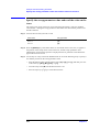
Agilent 4294A Precision Impedance Analyzer
Operation Manual
Fourth Edition
SERIAL NUMBERS
This manual applies directly to instruments that have
the serial number prefix JP1KG. For additional important
information about serial numbers, see Appendix A.
Part No. 04294-90030
January 2001
Printed in: Japan
Notices
The information contained in this document is subject to change without notice.
This document contains proprietary information that is protected by copyright. All
rights are reserved. No part of this document may be photocopied, reproduced, or
translated into another language without the prior written consent of Agilent
Technologies.
Agilent Technologies Japan, Ltd.
Kobe Instrument Division
1-3-2, Murotani, Nishi-Ku, Kobe-shi, Hyogo, 651-2241 Japan
© Copyright 1999, 2001 Agilent Technologies Japan, Ltd.
Manual Printing History
The manual’s printing date and part number indicate its current edition. The
printing date changes when a new edition is printed. (Minor corrections and
updates incorporated in reprints do not necessitate a new printing date.) The
manual part number changes when extensive technical changes are incorporated.
April 1999
First Edition
May 1999
Second Edition
December 1999
Third Edition
January 2001
Fourth Edition
Safety Summary
The following general safety precautions must be observed during all phases of
operation, service, and repair of this instrument. Failure to comply with these
precautions or with specific WARNINGS elsewhere in this manual may impair the
protection provided by the equipment. Such noncompliance would also violate
safety standards of design, manufacture, and intended use of the instrument.
The Agilent Technologies assumes no liability for the customer’s failure to comply
with these requirements.
2
NOTE
The Agilent 4294A complies with INSTALLATION CATEGORY II and
POLLUTION DEGREE 2 in IEC61010-1. The Agilent 4294A is an INDOOR
USE product.
NOTE
LEDs in the Agilent 4294A are Class 1 in accordance with IEC60825-1,
CLASS 1 LED PRODUCT.
•
Ground the Instrument
To avoid electric shock, the instrument chassis and cabinet must be grounded
with the supplied power cable’s grounding prong.
•
DO NOT Operate in an Explosive Atmosphere
Do not operate the instrument in the presence of inflammable gasses or fumes.
Operation of any electrical instrument in such an environment clearly
constitutes a safety hazard.
•
Keep Away from Live Circuits
Operators must not remove instrument covers. Component replacement and
internal adjustments must be made by qualified maintenance personnel. Do not
replace components with the power cable connected. Under certain conditions,
dangerous voltage levels may exist even with the power cable removed. To
avoid injuries, always disconnect the power and discharge circuits before
touching them.
•
DO NOT Service or Adjust Alone
Do not attempt internal service or adjustment unless another person, capable of
rendering first aid and resuscitation, is present.
•
DO NOT Substitute Parts or Modify the Instrument
To avoid the danger of introducing additional hazards, do not install substitute
parts or perform unauthorized modifications to the instrument. Return the
instrument to an Agilent Technologies Sales and Service Office for service and
repair to ensure that safety features are maintained in operational condition.
•
Dangerous Procedure Warnings
Warnings, such as the example below, precede potentially dangerous
procedures throughout this manual. Instructions contained in the warnings must
be followed.
WARNING
Dangerous voltage levels, capable of causing death, are present in this
instrument. Use extreme caution when handling, testing, or adjusting this
instrument.
3
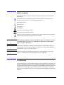
Safety Symbols
General definitions of safety symbols used on the instrument or in manuals are
listed below.
Instruction Manual symbol: the product is marked with this symbol when it is
necessary for the user to refer to the instrument manual.
Alternating current.
Direct current.
On (Supply).
Off (Supply).
In-position of push-button switch.
Out-position of push-button switch.
Frame (or chassis) terminal. A connection to the frame (chassis) of the equipment,
which normally includes all exposed metal structure.
WARNING
This warning sign denotes a hazard. It calls attention to a procedure, practice,
or condition that, if not correctly performed or adhered to, could result in
injury or death to personnel.
CAUTION
This Caution sign denotes a hazard. It calls attention to a procedure, practice, or
condition that, if not correctly performed or adhered to, could result in damage to
or destruction of part or all of the product.
NOTE
This Note sign denotes important information. It calls attention to a procedure,
practice, or condition that is essential for the user to understand.
Certification
Agilent Technologies certifies that this product met its published specifications at
the time of shipment from the factory. Agilent Technologies further certifies that
its calibration measurements are traceable to the United States National Institute of
Standards and Technology, to the extent allowed by the Institution’s calibration
facility or by the calibration facilities of other International Standards Organization
members.
4
Warranty
This Agilent Technologies instrument product is warranted against defects in
material and workmanship for a period corresponding to the individual warranty
periods of its component products. Instruments are warranted for a period of one
year. Fixtures and adapters are warranted for a period of 90 days. During the
warranty period, Agilent Technologies will, at its option, either repair or replace
products that prove to be defective.
For warranty service or repair, this product must be returned to a service facility
designated by Agilent Technologies. Buyer shall prepay shipping charges to
Agilent Technologies and Agilent Technologies shall pay shipping charges to
return the product to Buyer. However, Buyer shall pay all shipping charges, duties,
and taxes for products returned to Agilent Technologies from another country.
Agilent Technologies warrants that its software and firmware designated by
Agilent Technologies for use with an instrument will execute its programming
instruction when properly installed on that instrument. Agilent Technologies does
not warrant that the operation of the instrument, or software, or firmware will be
uninterrupted or error free.
Limitation of Warranty
The foregoing warranty shall not apply to defects resulting from improper or
inadequate maintenance by Buyer, Buyer-supplied software or interfacing,
unauthorized modification or misuse, operation outside the environmental
specifications for the product, or improper site preparation or maintenance.
IMPORTANT
No other warranty is expressed or implied. Agilent Technologies specifically
disclaims the implied warranties of merchantability and fitness for a particular
purpose.
Exclusive Remedies
The remedies provided herein are Buyer’s sole and exclusive remedies. Agilent
Technologies shall not be liable for any direct, indirect, special, incidental, or
consequential damages, whether based on contract, tort, or any other legal theory.
5
Assistance
Product maintenance agreements and other customer assistance agreements are
available for Agilent Technologies products.
For any assistance, contact your nearest Agilent Technologies Sales and Service
Office. Addresses are provided at the back of this manual.
Typeface Conventions
Bold
Boldface type is used when a term is defined.
For example: icons are symbols.
Italic
Italic type is used for emphasis and for titles
of manuals and other publications.
[Hardkey]
Indicates a hardkey labeled “Hardkey.”
Softkey
Indicates a softkey labeled “Softkey.”
[Hardkey]
- Softkey1 - Softkey2
Indicates keystrokes [Hardkey] - Softkey1 Softkey2.
Agilent 4294A Documentation Map
The following manuals are available for the Agilent 4294A.
•
Operation Manual (Agilent P/N: 04294-900x0)
Most of the basic information necessary for using the Agilent 4294A is
provided in this manual. It describes installation, preparation, measurement
operation including calibration, performances (specifications), key definitions,
and error messages. For GP-IB programming, see the Programming Manual
together with HP Instrument BASIC User's Handbook.
•
Programming Manual (Agilent P/N: 04294-900x1)
The Programming Manual shows how to write and use BASIC program to
control the Agilent 4294A and describes how HP Instrument BASIC works
with the analyzer.
•
6
HP Instrument BASIC User's Handbook (Agilent P/N: E2083-90005)
The HP Instrument BASIC User’s Handbook introduces you to the HP
Instrument BASIC programming language, provides some helpful hints on
getting the most use from it, and includes a general programming reference. It
is divided into three books: HP Instrument BASIC Programming Techniques,
HP Instrument BASIC Interface Techniques, and HP Instrument BASIC
Language Reference.
•
Service Manual (Agilent P/N: 04294-90100, Option 0BW only)
This manual explains how to adjust and repair the Agilent 4294A and how to
carry out performance tests. This manual is attached when Option 0BW is
ordered.
NOTE
The number of “x” in the part number of each manual (Agilent P/N), 0 for the first
edition, is incremented by 1 each time a revision is made.
7
8
Contents
1. Installation
Incoming Inspection . . . . . . . . . . . . . . . . . . . . . . . . . . . . . . . . . . . . . . . . . . . . . . . . . . . . . . . . . . . . . . . . . . . 18
Precautions to Take Before Setting Up the Power Supply . . . . . . . . . . . . . . . . . . . . . . . . . . . . . . . . . . . . . 20
Setting Up and Replacing the Fuse . . . . . . . . . . . . . . . . . . . . . . . . . . . . . . . . . . . . . . . . . . . . . . . . . . . . . 20
Power Source Requirements . . . . . . . . . . . . . . . . . . . . . . . . . . . . . . . . . . . . . . . . . . . . . . . . . . . . . . . . . . . 20
Power Cable . . . . . . . . . . . . . . . . . . . . . . . . . . . . . . . . . . . . . . . . . . . . . . . . . . . . . . . . . . . . . . . . . . . . . . . . . 21
Connecting the BNC Adapter (for Option 1D5 Only). . . . . . . . . . . . . . . . . . . . . . . . . . . . . . . . . . . . . . . . . 23
Using the LAN Port . . . . . . . . . . . . . . . . . . . . . . . . . . . . . . . . . . . . . . . . . . . . . . . . . . . . . . . . . . . . . . . . . . . 24
Connecting the Supplied Keyboard . . . . . . . . . . . . . . . . . . . . . . . . . . . . . . . . . . . . . . . . . . . . . . . . . . . . . . . 25
Using a Rackmount Kit. . . . . . . . . . . . . . . . . . . . . . . . . . . . . . . . . . . . . . . . . . . . . . . . . . . . . . . . . . . . . . . . . 26
Option 1CN Handle Kit. . . . . . . . . . . . . . . . . . . . . . . . . . . . . . . . . . . . . . . . . . . . . . . . . . . . . . . . . . . . . . . 26
Option 1CM Rackmount Kit . . . . . . . . . . . . . . . . . . . . . . . . . . . . . . . . . . . . . . . . . . . . . . . . . . . . . . . . . . . 27
Option 1CP Rackmount & Handle Kit . . . . . . . . . . . . . . . . . . . . . . . . . . . . . . . . . . . . . . . . . . . . . . . . . . . 27
Environmental Requirements . . . . . . . . . . . . . . . . . . . . . . . . . . . . . . . . . . . . . . . . . . . . . . . . . . . . . . . . . . . . 28
Ventilation Requirements . . . . . . . . . . . . . . . . . . . . . . . . . . . . . . . . . . . . . . . . . . . . . . . . . . . . . . . . . . . . . . . 28
Instructions for Cleaning . . . . . . . . . . . . . . . . . . . . . . . . . . . . . . . . . . . . . . . . . . . . . . . . . . . . . . . . . . . . . . . 28
2. Learning Operation Basics
Required Equipment . . . . . . . . . . . . . . . . . . . . . . . . . . . . . . . . . . . . . . . . . . . . . . . . . . . . . . . . . . . . . . . . . . . 30
Preparing for a Measurement . . . . . . . . . . . . . . . . . . . . . . . . . . . . . . . . . . . . . . . . . . . . . . . . . . . . . . . . . . . . 31
Connect the Agilent 16047E Test Fixture . . . . . . . . . . . . . . . . . . . . . . . . . . . . . . . . . . . . . . . . . . . . . . . . . 31
Turn ON the Power . . . . . . . . . . . . . . . . . . . . . . . . . . . . . . . . . . . . . . . . . . . . . . . . . . . . . . . . . . . . . . . . . . 32
Set the Adapter Type to “NONE” . . . . . . . . . . . . . . . . . . . . . . . . . . . . . . . . . . . . . . . . . . . . . . . . . . . . . . 32
Specifying Measurement Conditions . . . . . . . . . . . . . . . . . . . . . . . . . . . . . . . . . . . . . . . . . . . . . . . . . . . . . . 33
Initialize the Agilent 4294A to the Preset State . . . . . . . . . . . . . . . . . . . . . . . . . . . . . . . . . . . . . . . . . . . . 33
Select |Z|-θ as the Measurement Parameter . . . . . . . . . . . . . . . . . . . . . . . . . . . . . . . . . . . . . . . . . . . . . . . 33
Select Frequency as the Sweep Parameter . . . . . . . . . . . . . . . . . . . . . . . . . . . . . . . . . . . . . . . . . . . . . . . . 33
Select Logarithmic Sweep as the Sweep Type . . . . . . . . . . . . . . . . . . . . . . . . . . . . . . . . . . . . . . . . . . . . . 33
Set the Sweep Start Value to 100 Hz. . . . . . . . . . . . . . . . . . . . . . . . . . . . . . . . . . . . . . . . . . . . . . . . . . . . . 34
Set the Sweep Stop Value to 100 MHz . . . . . . . . . . . . . . . . . . . . . . . . . . . . . . . . . . . . . . . . . . . . . . . . . . . 34
Set the Measurement Bandwidth to 2 . . . . . . . . . . . . . . . . . . . . . . . . . . . . . . . . . . . . . . . . . . . . . . . . . . . . 34
Fixture Compensation. . . . . . . . . . . . . . . . . . . . . . . . . . . . . . . . . . . . . . . . . . . . . . . . . . . . . . . . . . . . . . . . . . 35
Perform Fixture Compensation for the Open Circuit State. . . . . . . . . . . . . . . . . . . . . . . . . . . . . . . . . . . . 35
Perform Fixture Compensation for the Short Circuit State. . . . . . . . . . . . . . . . . . . . . . . . . . . . . . . . . . . . 35
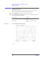
Carrying Out Measurement and Viewing Results . . . . . . . . . . . . . . . . . . . . . . . . . . . . . . . . . . . . . . . . . . . . 37
Connect the DUT . . . . . . . . . . . . . . . . . . . . . . . . . . . . . . . . . . . . . . . . . . . . . . . . . . . . . . . . . . . . . . . . . . . 37
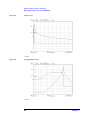
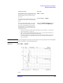
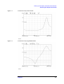
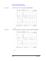
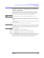
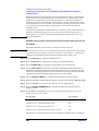
Apply the Logarithmic Format to the Vertical Axis for |Z| . . . . . . . . . . . . . . . . . . . . . . . . . . . . . . . . . . . . 38
Apply the Linear Format to the Vertical Axis for θ . . . . . . . . . . . . . . . . . . . . . . . . . . . . . . . . . . . . . . . . . 38
Display the Measured |Z| and θ Values in Parallel . . . . . . . . . . . . . . . . . . . . . . . . . . . . . . . . . . . . . . . . . . 39
Auto-scale the |Z| Trace. . . . . . . . . . . . . . . . . . . . . . . . . . . . . . . . . . . . . . . . . . . . . . . . . . . . . . . . . . . . . . . 40
Auto-scale the θ Trace. . . . . . . . . . . . . . . . . . . . . . . . . . . . . . . . . . . . . . . . . . . . . . . . . . . . . . . . . . . . . . . . 40
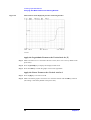
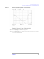
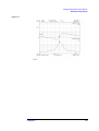
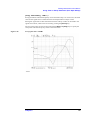
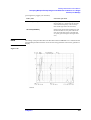
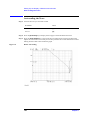
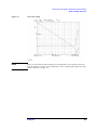
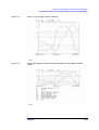
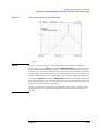
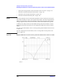
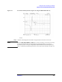
Results of Analysis . . . . . . . . . . . . . . . . . . . . . . . . . . . . . . . . . . . . . . . . . . . . . . . . . . . . . . . . . . . . . . . . . . . 42
Determine the Self-resonance Frequency and Resonant Impedance . . . . . . . . . . . . . . . . . . . . . . . . . . . . 42
3. Front/Rear Panel and LCD Display
Front Panel . . . . . . . . . . . . . . . . . . . . . . . . . . . . . . . . . . . . . . . . . . . . . . . . . . . . . . . . . . . . . . . . . . . . . . . . . . 44
Hardkeys . . . . . . . . . . . . . . . . . . . . . . . . . . . . . . . . . . . . . . . . . . . . . . . . . . . . . . . . . . . . . . . . . . . . . . . . . . 44
1. ACTIVE TRACE block . . . . . . . . . . . . . . . . . . . . . . . . . . . . . . . . . . . . . . . . . . . . . . . . . . . . . . . . . . . . 45
9
Contents
2. MEASUREMENT Block . . . . . . . . . . . . . . . . . . . . . . . . . . . . . . . . . . . . . . . . . . . . . . . . . . . . . . . . . .
3. STIMULUS Block . . . . . . . . . . . . . . . . . . . . . . . . . . . . . . . . . . . . . . . . . . . . . . . . . . . . . . . . . . . . . . . .
4. ENTRY Block . . . . . . . . . . . . . . . . . . . . . . . . . . . . . . . . . . . . . . . . . . . . . . . . . . . . . . . . . . . . . . . . . . .
5. MARKER Block. . . . . . . . . . . . . . . . . . . . . . . . . . . . . . . . . . . . . . . . . . . . . . . . . . . . . . . . . . . . . . . . . .
6. INSTRUMENT STATE Block . . . . . . . . . . . . . . . . . . . . . . . . . . . . . . . . . . . . . . . . . . . . . . . . . . . . . . .
7. Softkeys . . . . . . . . . . . . . . . . . . . . . . . . . . . . . . . . . . . . . . . . . . . . . . . . . . . . . . . . . . . . . . . . . . . . . . . .
8. Color LCD Display . . . . . . . . . . . . . . . . . . . . . . . . . . . . . . . . . . . . . . . . . . . . . . . . . . . . . . . . . . . . . . . .
9. Power Switch . . . . . . . . . . . . . . . . . . . . . . . . . . . . . . . . . . . . . . . . . . . . . . . . . . . . . . . . . . . . . . . . . . . .
10. UNKNOWN Terminals . . . . . . . . . . . . . . . . . . . . . . . . . . . . . . . . . . . . . . . . . . . . . . . . . . . . . . . . . . .
11. Built-in 3.5 Inch Floppy Disk Drive . . . . . . . . . . . . . . . . . . . . . . . . . . . . . . . . . . . . . . . . . . . . . . . . . .
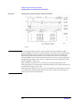
Rear Panel. . . . . . . . . . . . . . . . . . . . . . . . . . . . . . . . . . . . . . . . . . . . . . . . . . . . . . . . . . . . . . . . . . . . . . . . . . .
1. External Reference Input Connector. . . . . . . . . . . . . . . . . . . . . . . . . . . . . . . . . . . . . . . . . . . . . . . . . . .
2. High Stability Frequency Reference (Option 1D5 Only) . . . . . . . . . . . . . . . . . . . . . . . . . . . . . . . . . . .
3. External Trigger Input. . . . . . . . . . . . . . . . . . . . . . . . . . . . . . . . . . . . . . . . . . . . . . . . . . . . . . . . . . . . . .
4. LAN Port. . . . . . . . . . . . . . . . . . . . . . . . . . . . . . . . . . . . . . . . . . . . . . . . . . . . . . . . . . . . . . . . . . . . . . . .
5. Internal Reference Output. . . . . . . . . . . . . . . . . . . . . . . . . . . . . . . . . . . . . . . . . . . . . . . . . . . . . . . . . . .
6. External Program RUN/CONT Input . . . . . . . . . . . . . . . . . . . . . . . . . . . . . . . . . . . . . . . . . . . . . . . . . .
7. 8-bit I/O Port . . . . . . . . . . . . . . . . . . . . . . . . . . . . . . . . . . . . . . . . . . . . . . . . . . . . . . . . . . . . . . . . . . . .
8. Time Base Adjuster (for Option 1D5) . . . . . . . . . . . . . . . . . . . . . . . . . . . . . . . . . . . . . . . . . . . . . . . . .
9. Mini-DIN Keyboard Port. . . . . . . . . . . . . . . . . . . . . . . . . . . . . . . . . . . . . . . . . . . . . . . . . . . . . . . . . . .
10. 24-bit I/O Port. . . . . . . . . . . . . . . . . . . . . . . . . . . . . . . . . . . . . . . . . . . . . . . . . . . . . . . . . . . . . . . . . . .
11. Printer Port . . . . . . . . . . . . . . . . . . . . . . . . . . . . . . . . . . . . . . . . . . . . . . . . . . . . . . . . . . . . . . . . . . . . .
12. External Monitor Terminal . . . . . . . . . . . . . . . . . . . . . . . . . . . . . . . . . . . . . . . . . . . . . . . . . . . . . . . . .
13. GPIB Connector . . . . . . . . . . . . . . . . . . . . . . . . . . . . . . . . . . . . . . . . . . . . . . . . . . . . . . . . . . . . . . . . .
14. Inlet (with a fuse box) . . . . . . . . . . . . . . . . . . . . . . . . . . . . . . . . . . . . . . . . . . . . . . . . . . . . . . . . . . . . .
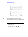
Items Displayed on the LCD . . . . . . . . . . . . . . . . . . . . . . . . . . . . . . . . . . . . . . . . . . . . . . . . . . . . . . . . . . . .
1. Measurement Parameter Fields. . . . . . . . . . . . . . . . . . . . . . . . . . . . . . . . . . . . . . . . . . . . . . . . . . . . . . .
2. Scale/Reference Fields . . . . . . . . . . . . . . . . . . . . . . . . . . . . . . . . . . . . . . . . . . . . . . . . . . . . . . . . . . . . .
3. Marker Measurement Parameter Value Fields . . . . . . . . . . . . . . . . . . . . . . . . . . . . . . . . . . . . . . . . . . .
4. Menu Title Field . . . . . . . . . . . . . . . . . . . . . . . . . . . . . . . . . . . . . . . . . . . . . . . . . . . . . . . . . . . . . . . . . .
5. Softkey Label Area . . . . . . . . . . . . . . . . . . . . . . . . . . . . . . . . . . . . . . . . . . . . . . . . . . . . . . . . . . . . . . . .
6. Sweep Parameter Reading Fields . . . . . . . . . . . . . . . . . . . . . . . . . . . . . . . . . . . . . . . . . . . . . . . . . . . . .
7. Marker Status Fields . . . . . . . . . . . . . . . . . . . . . . . . . . . . . . . . . . . . . . . . . . . . . . . . . . . . . . . . . . . . . . .
8. Marker Statistics/Trace Bandwidth Analysis Fields. . . . . . . . . . . . . . . . . . . . . . . . . . . . . . . . . . . . . . .
9. Limit Line Test Fields. . . . . . . . . . . . . . . . . . . . . . . . . . . . . . . . . . . . . . . . . . . . . . . . . . . . . . . . . . . . . .
10. HP Instrument Basic Status Indicator . . . . . . . . . . . . . . . . . . . . . . . . . . . . . . . . . . . . . . . . . . . . . . . . .
11. dc Voltage/Current Bias Monitor Field. . . . . . . . . . . . . . . . . . . . . . . . . . . . . . . . . . . . . . . . . . . . . . . .
12. Sweep Stop/Span Value Field . . . . . . . . . . . . . . . . . . . . . . . . . . . . . . . . . . . . . . . . . . . . . . . . . . . . . . .
13. Test Signal Current Level Monitor Field . . . . . . . . . . . . . . . . . . . . . . . . . . . . . . . . . . . . . . . . . . . . . .
14. Test Signal Level/CW Frequency Setting Field . . . . . . . . . . . . . . . . . . . . . . . . . . . . . . . . . . . . . . . . .
15. Test Signal Voltage Level Monitor Field . . . . . . . . . . . . . . . . . . . . . . . . . . . . . . . . . . . . . . . . . . . . . .
16. Sweep Start/Center Value Field . . . . . . . . . . . . . . . . . . . . . . . . . . . . . . . . . . . . . . . . . . . . . . . . . . . . .
17. Instrument Status Area . . . . . . . . . . . . . . . . . . . . . . . . . . . . . . . . . . . . . . . . . . . . . . . . . . . . . . . . . . . .
18. Equivalent Circuit Parameters Field . . . . . . . . . . . . . . . . . . . . . . . . . . . . . . . . . . . . . . . . . . . . . . . . . .
19. External Reference Input Status Field . . . . . . . . . . . . . . . . . . . . . . . . . . . . . . . . . . . . . . . . . . . . . . . .
20. Parameter Setting/Instrument Message Field . . . . . . . . . . . . . . . . . . . . . . . . . . . . . . . . . . . . . . . . . . .
21. Title Field . . . . . . . . . . . . . . . . . . . . . . . . . . . . . . . . . . . . . . . . . . . . . . . . . . . . . . . . . . . . . . . . . . . . . .
4. Preparation of Measurement Accessories
10
45
46
46
47
47
48
48
48
49
49
50
50
50
51
51
51
51
51
51
51
52
52
52
52
52
53
53
53
53
53
54
55
55
56
56
56
56
57
57
57
57
57
57
60
60
60
61
Contents
Selecting Accessories for Measurement . . . . . . . . . . . . . . . . . . . . . . . . . . . . . . . . . . . . . . . . . . . . . . . . . . . . 64
Connecting the Accessories . . . . . . . . . . . . . . . . . . . . . . . . . . . . . . . . . . . . . . . . . . . . . . . . . . . . . . . . . . . . . 66
Adapter Setting . . . . . . . . . . . . . . . . . . . . . . . . . . . . . . . . . . . . . . . . . . . . . . . . . . . . . . . . . . . . . . . . . . . . . . . 67
Adapter Selection . . . . . . . . . . . . . . . . . . . . . . . . . . . . . . . . . . . . . . . . . . . . . . . . . . . . . . . . . . . . . . . . . . . 68
Adapter Setup . . . . . . . . . . . . . . . . . . . . . . . . . . . . . . . . . . . . . . . . . . . . . . . . . . . . . . . . . . . . . . . . . . . . . . 69
Adapter Setup Procedure for the 16048G and 16048H. . . . . . . . . . . . . . . . . . . . . . . . . . . . . . . . . . . . . . . 70
Adapter Setup Procedure for the 16334A . . . . . . . . . . . . . . . . . . . . . . . . . . . . . . . . . . . . . . . . . . . . . . . . . 72
Adapter Setup Procedure for the 16451B . . . . . . . . . . . . . . . . . . . . . . . . . . . . . . . . . . . . . . . . . . . . . . . . . 73
Adapter Setup Procedure for the 42942A . . . . . . . . . . . . . . . . . . . . . . . . . . . . . . . . . . . . . . . . . . . . . . . . . 74
Adapter Setup Procedure for the 42941A . . . . . . . . . . . . . . . . . . . . . . . . . . . . . . . . . . . . . . . . . . . . . . . . . 78
5. Setting Measurement Conditions
Putting the Agilent 4294A into the Preset State (Presetting) . . . . . . . . . . . . . . . . . . . . . . . . . . . . . . . . . . . . 82
Selecting Trace (Active Trace) . . . . . . . . . . . . . . . . . . . . . . . . . . . . . . . . . . . . . . . . . . . . . . . . . . . . . . . . . . 83
Selecting Sweep Parameter. . . . . . . . . . . . . . . . . . . . . . . . . . . . . . . . . . . . . . . . . . . . . . . . . . . . . . . . . . . . . . 84
Selecting Linear, Log, or List Sweep . . . . . . . . . . . . . . . . . . . . . . . . . . . . . . . . . . . . . . . . . . . . . . . . . . . . . . 87
Setting Sweep Range . . . . . . . . . . . . . . . . . . . . . . . . . . . . . . . . . . . . . . . . . . . . . . . . . . . . . . . . . . . . . . . . . . 89
Setting by start and stop values . . . . . . . . . . . . . . . . . . . . . . . . . . . . . . . . . . . . . . . . . . . . . . . . . . . . . . . . . 89
Setting by center and span values . . . . . . . . . . . . . . . . . . . . . . . . . . . . . . . . . . . . . . . . . . . . . . . . . . . . . . . 89
Setting sweep range with marker . . . . . . . . . . . . . . . . . . . . . . . . . . . . . . . . . . . . . . . . . . . . . . . . . . . . . . . 90
Using Time as Sweep Parameter (Zero Span Sweep) . . . . . . . . . . . . . . . . . . . . . . . . . . . . . . . . . . . . . . . . . 94
Setting Number of Points (NOP) . . . . . . . . . . . . . . . . . . . . . . . . . . . . . . . . . . . . . . . . . . . . . . . . . . . . . . . . . 97
Selecting Sweep Direction . . . . . . . . . . . . . . . . . . . . . . . . . . . . . . . . . . . . . . . . . . . . . . . . . . . . . . . . . . . . . . 99
Manual Sweep (Measurement at a Specified Point) . . . . . . . . . . . . . . . . . . . . . . . . . . . . . . . . . . . . . . . . . 100
Setting Time Delay for Measurement. . . . . . . . . . . . . . . . . . . . . . . . . . . . . . . . . . . . . . . . . . . . . . . . . . . . . 102
Setting with sweep time . . . . . . . . . . . . . . . . . . . . . . . . . . . . . . . . . . . . . . . . . . . . . . . . . . . . . . . . . . . . . 102
Setting with time delay at measurement point . . . . . . . . . . . . . . . . . . . . . . . . . . . . . . . . . . . . . . . . . . . . 102
Setting with sweep time delay. . . . . . . . . . . . . . . . . . . . . . . . . . . . . . . . . . . . . . . . . . . . . . . . . . . . . . . . . 103
Setting Fixed Frequency (CW Frequency) . . . . . . . . . . . . . . . . . . . . . . . . . . . . . . . . . . . . . . . . . . . . . . . . . 104
Setting Oscillator Level . . . . . . . . . . . . . . . . . . . . . . . . . . . . . . . . . . . . . . . . . . . . . . . . . . . . . . . . . . . . . . . 105
Selecting Unit for Oscillator Level (Voltage or Current) . . . . . . . . . . . . . . . . . . . . . . . . . . . . . . . . . . . . . . 106
Setting and Applying dc Bias . . . . . . . . . . . . . . . . . . . . . . . . . . . . . . . . . . . . . . . . . . . . . . . . . . . . . . . . . . . 107
1. Selecting dc bias mode . . . . . . . . . . . . . . . . . . . . . . . . . . . . . . . . . . . . . . . . . . . . . . . . . . . . . . . . . . . . 107
2. Setting fixed dc bias level . . . . . . . . . . . . . . . . . . . . . . . . . . . . . . . . . . . . . . . . . . . . . . . . . . . . . . . . . . 107
3. Setting limits for dc voltage . . . . . . . . . . . . . . . . . . . . . . . . . . . . . . . . . . . . . . . . . . . . . . . . . . . . . . . . 108
4. Setting dc bias range to 1 mA . . . . . . . . . . . . . . . . . . . . . . . . . . . . . . . . . . . . . . . . . . . . . . . . . . . . . . . 108
5. Turning dc bias ON or OFF . . . . . . . . . . . . . . . . . . . . . . . . . . . . . . . . . . . . . . . . . . . . . . . . . . . . . . . . 109
6. Optimizing dc bias range. . . . . . . . . . . . . . . . . . . . . . . . . . . . . . . . . . . . . . . . . . . . . . . . . . . . . . . . . . . 109
Selecting a Method to Start Measurement (Trigger Source) . . . . . . . . . . . . . . . . . . . . . . . . . . . . . . . . . . . 111
Selecting Sweep Trigger/Measurement Point Trigger . . . . . . . . . . . . . . . . . . . . . . . . . . . . . . . . . . . . . . . . 112
Selecting Polarity of External Trigger Input Signal . . . . . . . . . . . . . . . . . . . . . . . . . . . . . . . . . . . . . . . . . . 113
Specifying Sweep Times and Stopping Sweep. . . . . . . . . . . . . . . . . . . . . . . . . . . . . . . . . . . . . . . . . . . . . . 114
Single sweep . . . . . . . . . . . . . . . . . . . . . . . . . . . . . . . . . . . . . . . . . . . . . . . . . . . . . . . . . . . . . . . . . . . . . . 114
Sweep by specified times . . . . . . . . . . . . . . . . . . . . . . . . . . . . . . . . . . . . . . . . . . . . . . . . . . . . . . . . . . . . 114
Sweep with unlimited times (continuous sweep) . . . . . . . . . . . . . . . . . . . . . . . . . . . . . . . . . . . . . . . . . . 115
Stopping sweep . . . . . . . . . . . . . . . . . . . . . . . . . . . . . . . . . . . . . . . . . . . . . . . . . . . . . . . . . . . . . . . . . . . . 115
Sweeping Multiple Sweep Ranges with Different Conditions in a Single Action (List Sweep) . . . . . . . . 116
Preparing list sweep table . . . . . . . . . . . . . . . . . . . . . . . . . . . . . . . . . . . . . . . . . . . . . . . . . . . . . . . . . . . . 118
Selecting the list sweep as the sweep type . . . . . . . . . . . . . . . . . . . . . . . . . . . . . . . . . . . . . . . . . . . . . . . 124
11
Contents
Setting the Horizontal Axis of the Graph for the List Sweep . . . . . . . . . . . . . . . . . . . . . . . . . . . . . . . . .
Setting Measurement Accuracy, Stability, and Time . . . . . . . . . . . . . . . . . . . . . . . . . . . . . . . . . . . . . . . . .
Setting measurement bandwidth . . . . . . . . . . . . . . . . . . . . . . . . . . . . . . . . . . . . . . . . . . . . . . . . . . . . . . .
Averaging between sweeps (sweep-to-sweep averaging) . . . . . . . . . . . . . . . . . . . . . . . . . . . . . . . . . . .
Averaging for each measurement point (point averaging) . . . . . . . . . . . . . . . . . . . . . . . . . . . . . . . . . . .
124
126
126
126
127
6. Calibration
Selecting Appropriate Calibration Method . . . . . . . . . . . . . . . . . . . . . . . . . . . . . . . . . . . . . . . . . . . . . . . .
A. Calibration When Using Direct Connection Type Test Fixture. . . . . . . . . . . . . . . . . . . . . . . . . . . . . . .
B. Calibration for Four-Terminal Pair, 1-m Extension. . . . . . . . . . . . . . . . . . . . . . . . . . . . . . . . . . . . . . . .
Fixture Compensation When the 16451B is Used . . . . . . . . . . . . . . . . . . . . . . . . . . . . . . . . . . . . . . . . .
C. Calibration for Four-Terminal Pair, 2-m Extension. . . . . . . . . . . . . . . . . . . . . . . . . . . . . . . . . . . . . . . .
D. Calibration When an Exclusive Fixture is Connected to the 42942A. . . . . . . . . . . . . . . . . . . . . . . . . .
E. Calibration When the 7-mm Port of the 42942A is Extended . . . . . . . . . . . . . . . . . . . . . . . . . . . . . . . .
F. Calibration When a Probe Adapter is Connected to the 42941A . . . . . . . . . . . . . . . . . . . . . . . . . . . . . .
G. Calibration When the 3.5-mm Port of the 42941A is Extended . . . . . . . . . . . . . . . . . . . . . . . . . . . . . .
User Calibration . . . . . . . . . . . . . . . . . . . . . . . . . . . . . . . . . . . . . . . . . . . . . . . . . . . . . . . . . . . . . . . . . . . . .
User Calibration Procedure. . . . . . . . . . . . . . . . . . . . . . . . . . . . . . . . . . . . . . . . . . . . . . . . . . . . . . . . . . .
Turning User Calibration On/Off . . . . . . . . . . . . . . . . . . . . . . . . . . . . . . . . . . . . . . . . . . . . . . . . . . . . . .
Defining Standard Values for User Calibration . . . . . . . . . . . . . . . . . . . . . . . . . . . . . . . . . . . . . . . . . . .
Port Extension Compensation . . . . . . . . . . . . . . . . . . . . . . . . . . . . . . . . . . . . . . . . . . . . . . . . . . . . . . . . . .
Fixture Compensation . . . . . . . . . . . . . . . . . . . . . . . . . . . . . . . . . . . . . . . . . . . . . . . . . . . . . . . . . . . . . . . .
Fixture compensation procedure. . . . . . . . . . . . . . . . . . . . . . . . . . . . . . . . . . . . . . . . . . . . . . . . . . . . . . .
Turning the fixture compensation on or off . . . . . . . . . . . . . . . . . . . . . . . . . . . . . . . . . . . . . . . . . . . . . .
Defining the standard values for fixture compensation . . . . . . . . . . . . . . . . . . . . . . . . . . . . . . . . . . . . .
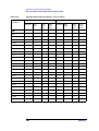
Selecting Calibration/Compensation Data Points . . . . . . . . . . . . . . . . . . . . . . . . . . . . . . . . . . . . . . . . . . .
List of fixed calibration/compensation frequency points . . . . . . . . . . . . . . . . . . . . . . . . . . . . . . . . . . . .
130
133
135
136
137
139
141
143
145
147
147
148
148
150
151
151
152
152
155
156
7. Setting Up the Display of Measurement Results
Selecting the Measurement Parameters . . . . . . . . . . . . . . . . . . . . . . . . . . . . . . . . . . . . . . . . . . . . . . . . . . .
Selecting the Graph Axis Format . . . . . . . . . . . . . . . . . . . . . . . . . . . . . . . . . . . . . . . . . . . . . . . . . . . . . . . .
When Using Cartesian Coordinates . . . . . . . . . . . . . . . . . . . . . . . . . . . . . . . . . . . . . . . . . . . . . . . . . . . .
When Using Complex Parameters (COMPLEX Z-Y) . . . . . . . . . . . . . . . . . . . . . . . . . . . . . . . . . . . . . .
Auto-scaling the Trace . . . . . . . . . . . . . . . . . . . . . . . . . . . . . . . . . . . . . . . . . . . . . . . . . . . . . . . . . . . . . . . .
Manual Scale Setting (for measurements other than COMPLEX Z-Y). . . . . . . . . . . . . . . . . . . . . . . . . . .
Scaling the Trace Based on the Reference Line and Resolution per Division . . . . . . . . . . . . . . . . . . . .
Scaling the Trace Based on the Top and Bottom Values . . . . . . . . . . . . . . . . . . . . . . . . . . . . . . . . . . . .
Manually Scaling the Active Trace for a COMPLEX Z-Y Graph . . . . . . . . . . . . . . . . . . . . . . . . . . . . . . .
Scaling the Active Trace for a Complex Plane . . . . . . . . . . . . . . . . . . . . . . . . . . . . . . . . . . . . . . . . . . . .
Scaling the Active Trace for a Polar Chart . . . . . . . . . . . . . . . . . . . . . . . . . . . . . . . . . . . . . . . . . . . . . . .
Selecting the Target Trace Type (Data or Memory) . . . . . . . . . . . . . . . . . . . . . . . . . . . . . . . . . . . . . . . . . .
Enabling or Disabling Coupled Scaling Mode. . . . . . . . . . . . . . . . . . . . . . . . . . . . . . . . . . . . . . . . . . . . . .
Trace-based Comparison and Calculation . . . . . . . . . . . . . . . . . . . . . . . . . . . . . . . . . . . . . . . . . . . . . . . . .
Identifying Differences between Data and Memory Traces through Comparison or Calculation . . . . .
Subtracting an Offset Value . . . . . . . . . . . . . . . . . . . . . . . . . . . . . . . . . . . . . . . . . . . . . . . . . . . . . . . . . .
Superimposing Multiple Traces . . . . . . . . . . . . . . . . . . . . . . . . . . . . . . . . . . . . . . . . . . . . . . . . . . . . . . . . .
Comparing traces using the list sweep function . . . . . . . . . . . . . . . . . . . . . . . . . . . . . . . . . . . . . . . . . . .
Monitoring the Test Signal Level (AC) . . . . . . . . . . . . . . . . . . . . . . . . . . . . . . . . . . . . . . . . . . . . . . . . . . .
158
160
160
162
164
166
166
169
172
172
175
177
178
179
179
184
185
186
189
12
Contents
Monitoring the Test Signal Level on a Real-time Basis . . . . . . . . . . . . . . . . . . . . . . . . . . . . . . . . . . . . . 189
Using the Marker Feature to Determine the Test Signal Level. . . . . . . . . . . . . . . . . . . . . . . . . . . . . . . . 190
Monitoring the dc Bias Level . . . . . . . . . . . . . . . . . . . . . . . . . . . . . . . . . . . . . . . . . . . . . . . . . . . . . . . . . . . 193
Monitoring the dc Bias Level on a Real-time Basis . . . . . . . . . . . . . . . . . . . . . . . . . . . . . . . . . . . . . . . . 193
Using the Marker Feature to Determine the dc Bias Level. . . . . . . . . . . . . . . . . . . . . . . . . . . . . . . . . . . 194
Selecting the Phase Unit . . . . . . . . . . . . . . . . . . . . . . . . . . . . . . . . . . . . . . . . . . . . . . . . . . . . . . . . . . . . . . . 197
Displaying Phase Values without Wrapping at ±180° . . . . . . . . . . . . . . . . . . . . . . . . . . . . . . . . . . . . . . . . 198
Hiding the Non-active Trace. . . . . . . . . . . . . . . . . . . . . . . . . . . . . . . . . . . . . . . . . . . . . . . . . . . . . . . . . . . . 199
Splitting the Graph . . . . . . . . . . . . . . . . . . . . . . . . . . . . . . . . . . . . . . . . . . . . . . . . . . . . . . . . . . . . . . . . . . . 200
Configuring the Screen Assignments for HP Instrument BASIC. . . . . . . . . . . . . . . . . . . . . . . . . . . . . . . . 202
Adding a Title to the Measurement Screen. . . . . . . . . . . . . . . . . . . . . . . . . . . . . . . . . . . . . . . . . . . . . . . . . 205
Customizing Intensity and Color Settings for Screen Display . . . . . . . . . . . . . . . . . . . . . . . . . . . . . . . . . . 207
Setting the Foreground Intensity . . . . . . . . . . . . . . . . . . . . . . . . . . . . . . . . . . . . . . . . . . . . . . . . . . . . . . . 207
Adjusting the Background Intensity . . . . . . . . . . . . . . . . . . . . . . . . . . . . . . . . . . . . . . . . . . . . . . . . . . . . 207
Customizing the Color of Each Screen Item. . . . . . . . . . . . . . . . . . . . . . . . . . . . . . . . . . . . . . . . . . . . . . 208
Resetting All Items to Factory Default Colors . . . . . . . . . . . . . . . . . . . . . . . . . . . . . . . . . . . . . . . . . . . . 210
8. Analysis and Processing of Result
Specify the sweep parameter value and read the value on the trace. . . . . . . . . . . . . . . . . . . . . . . . . . . . . . 212
Listing data at several points on the trace. . . . . . . . . . . . . . . . . . . . . . . . . . . . . . . . . . . . . . . . . . . . . . . . . . 214
Displaying several marker positions using softkey labels . . . . . . . . . . . . . . . . . . . . . . . . . . . . . . . . . . . 214
Listing the marker positions with the marker list function . . . . . . . . . . . . . . . . . . . . . . . . . . . . . . . . . . . 215
Reading the difference from the reference point on the screen (delta marker) . . . . . . . . . . . . . . . . . . . . . 217
Placing the delta marker on the reference point with the main marker. . . . . . . . . . . . . . . . . . . . . . . . . . 217
Moving the delta marker alone to place it at a reference point . . . . . . . . . . . . . . . . . . . . . . . . . . . . . . . . 218
Displaying the main/sub-marker and reading the difference from the reference point. . . . . . . . . . . . . . 219
Reading actual measurement points only/reading interpolated values between measurement points . . . . 222
Search the maximum/minimum measurements . . . . . . . . . . . . . . . . . . . . . . . . . . . . . . . . . . . . . . . . . . . . . 223
Search the point of target measurement . . . . . . . . . . . . . . . . . . . . . . . . . . . . . . . . . . . . . . . . . . . . . . . . . . . 225
Search the maximum/minimum peak . . . . . . . . . . . . . . . . . . . . . . . . . . . . . . . . . . . . . . . . . . . . . . . . . . . . . 228
Define the Peak. . . . . . . . . . . . . . . . . . . . . . . . . . . . . . . . . . . . . . . . . . . . . . . . . . . . . . . . . . . . . . . . . . . . . . 232
Definition of peak polarity . . . . . . . . . . . . . . . . . . . . . . . . . . . . . . . . . . . . . . . . . . . . . . . . . . . . . . . . . . . 232
Define peak sharpness. . . . . . . . . . . . . . . . . . . . . . . . . . . . . . . . . . . . . . . . . . . . . . . . . . . . . . . . . . . . . . . 233
Define peak sharpness using a peak on the trace . . . . . . . . . . . . . . . . . . . . . . . . . . . . . . . . . . . . . . . . . . 233
Automatically performing search for each sweep (search tracking) . . . . . . . . . . . . . . . . . . . . . . . . . . . . . 235
Analyze trace bandwidth . . . . . . . . . . . . . . . . . . . . . . . . . . . . . . . . . . . . . . . . . . . . . . . . . . . . . . . . . . . . . . 236
Definitions of parameters in the trace bandwidth analysis . . . . . . . . . . . . . . . . . . . . . . . . . . . . . . . . . . . 236
Define the cutoff point in trace bandwidth analysis . . . . . . . . . . . . . . . . . . . . . . . . . . . . . . . . . . . . . . . . 238
Setting the delta marker in the trace bandwidth analysis . . . . . . . . . . . . . . . . . . . . . . . . . . . . . . . . . . . . 239
Implement trace bandwidth analysis . . . . . . . . . . . . . . . . . . . . . . . . . . . . . . . . . . . . . . . . . . . . . . . . . . . . 240
Set the marker separately for either trace A or B . . . . . . . . . . . . . . . . . . . . . . . . . . . . . . . . . . . . . . . . . . . . 243
Selecting target trace (data or memory) for marker analysis . . . . . . . . . . . . . . . . . . . . . . . . . . . . . . . . . . . 244
Selecting the sweep parameter value of the marker display as time from start or relaxation time . . . . . . 245
Clearing (turning off) the marker from the screen . . . . . . . . . . . . . . . . . . . . . . . . . . . . . . . . . . . . . . . . . . . 247
Turning off the sub-markers . . . . . . . . . . . . . . . . . . . . . . . . . . . . . . . . . . . . . . . . . . . . . . . . . . . . . . . . . . 247
Turning off the delta marker . . . . . . . . . . . . . . . . . . . . . . . . . . . . . . . . . . . . . . . . . . . . . . . . . . . . . . . . . . 247
Turning off all (main/sub/delta) markers at one time . . . . . . . . . . . . . . . . . . . . . . . . . . . . . . . . . . . . . . . 248
Calculate the equivalent circuit parameter and simulate the frequency characteristics . . . . . . . . . . . . . . . 249
Calculate the equivalent circuit parameter based on the measurement result. . . . . . . . . . . . . . . . . . . . . 249
13
Contents
Simulate the frequency characteristics based on the equivalent circuit parameter. . . . . . . . . . . . . . . . . 252
Calculating the mean value, standard deviation, and peak-to-peak of the trace . . . . . . . . . . . . . . . . . . . . 254
Set a limit to the trace and make pass/fail evaluation . . . . . . . . . . . . . . . . . . . . . . . . . . . . . . . . . . . . . . . . 256
Set the limit line . . . . . . . . . . . . . . . . . . . . . . . . . . . . . . . . . . . . . . . . . . . . . . . . . . . . . . . . . . . . . . . . . . . 256
Conduct the limit line test. . . . . . . . . . . . . . . . . . . . . . . . . . . . . . . . . . . . . . . . . . . . . . . . . . . . . . . . . . . . 262
Move the limit line in vertical and horizontal directions on the screen . . . . . . . . . . . . . . . . . . . . . . . . . 264
Specify partial search range . . . . . . . . . . . . . . . . . . . . . . . . . . . . . . . . . . . . . . . . . . . . . . . . . . . . . . . . . . . . 267
When sweep type is other than list sweep: . . . . . . . . . . . . . . . . . . . . . . . . . . . . . . . . . . . . . . . . . . . . . . . 267
When the sweep type is list sweep: . . . . . . . . . . . . . . . . . . . . . . . . . . . . . . . . . . . . . . . . . . . . . . . . . . . . 269
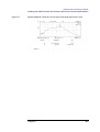
Save and Recall the Agilent 4294A Internal Data . . . . . . . . . . . . . . . . . . . . . . . . . . . . . . . . . . . . . . . . . . . 270
Agilent 4294A internal data flow . . . . . . . . . . . . . . . . . . . . . . . . . . . . . . . . . . . . . . . . . . . . . . . . . . . . . 270
Save the setting state, calibration data and memory array (State Save) . . . . . . . . . . . . . . . . . . . . . . . . . 271
Save the calibration data and trace data (Data Save) . . . . . . . . . . . . . . . . . . . . . . . . . . . . . . . . . . . . . . . 273
Using files saved in the text (ASCII) format with the data save function . . . . . . . . . . . . 275
Save the display screen (Graphic Save) . . . . . . . . . . . . . . . . . . . . . . . . . . . . . . . . . . . . . . . . . . . . . . . . . 285
Overwrite on the file to be saved . . . . . . . . . . . . . . . . . . . . . . . . . . . . . . . . . . . . . . . . . . . . . . . . . . . . . . 286
Create a file for automatic setting when power is on . . . . . . . . . . . . . . . . . . . . . . . . . . . . . . . . . . . . . . . 288
Recall the saved file . . . . . . . . . . . . . . . . . . . . . . . . . . . . . . . . . . . . . . . . . . . . . . . . . . . . . . . . . . . . . . . . 288
Print the measurement results and internal data with a printer . . . . . . . . . . . . . . . . . . . . . . . . . . . . . . . . . 291
Set the print form (color, resolution and how to handle the paper) . . . . . . . . . . . . . . . . . . . . . . . . . . . . 291
Print the measurements in graphic representation . . . . . . . . . . . . . . . . . . . . . . . . . . . . . . . . . . . . . . . . . 293
Print the measurements and settings (text) . . . . . . . . . . . . . . . . . . . . . . . . . . . . . . . . . . . . . . . . . . . . . . . 293
9. Setting/Using Control and Management Functions
Re-displaying an Instrument Message . . . . . . . . . . . . . . . . . . . . . . . . . . 298
Setting/Checking the Internal Clock . . . . . . . . . . . . . . . . . . . . . . . . . . . 299
Setting/Checking the Date . . . . . . . . . . . . . . . . . . . . . . . . . . . . . . 299
Setting/Checking the Time . . . . . . . . . . . . . . . . . . . . . . . . . . . . . . 300
Setting the Built-in Speaker (Beep Sound) . . . . . . . . . . . . . . . . . . . . . . . . 302
Turning On/Off the Completion Beep . . . . . . . . . . . . . . . . . . . . . . . . . . . . . . . . . . . . . . . . . . . . . . . . . . 302
Turning On/Off the Warning Beep . . . . . . . . . . . . . . . . . . . . . . . . . . . . . . . . . . . . . . . . . . . . . . . . . . . . . 302
Managing Files . . . . . . . . . . . . . . . . . . . . . . . . . . . . . . . . . . . 304
Creating a Directory . . . . . . . . . . . . . . . . . . . . . . . . . . . . . . . . 304
Copying a File. . . . . . . . . . . . . . . . . . . . . . . . . . . . . . . . . . . 306
Deleting a File or Directory . . . . . . . . . . . . . . . . . . . . . . . . . . . . . 309
Initializing a Recording Medium . . . . . . . . . . . . . . . . . . . . . . . . . . . 310
Setting/Checking the GP-IB . . . . . . . . . . . . . . . . . . . . . . . . . . . . . . 312
Switching between the System Controller Mode and Addressable-only Mode . . . . . . . . . . 312
Setting/Checking the GP-IB address . . . . . . . . . . . . . . . . . . . . . . . . . . 312
Setting/Checking the LAN . . . . . . . . . . . . . . . . . . . . . . . . . . . . . . . 314
Setting/Checking the IP Address . . . . . . . . . . . . . . . . . . . . . . . . . . . 314
Setting/Checking the Gateway Address . . . . . . . . . . . . . . . . . . . . . . . . . 315
Setting/Checking the Subnet Mask. . . . . . . . . . . . . . . . . . . . . . . . . . . 317
Checking the MAC Address . . . . . . . . . . . . . . . . . . . . . . . . . . . . . 318
Checking the Firmware Version . . . . . . . . . . . . . . . . . . . . . . . . . . . . . 319
Checking by Key Operation . . . . . . . . . . . . . . . . . . . . . . . . . . . . . . . . . . . . . . . . . . . . . . . . . . . . . . . . . . 319
Checking by Powering On Again . . . . . . . . . . . . . . . . . . . . . . . . . . . . . . . . . . . . . . . . . . . . . . . . . . . . . . 319
Performing Self-Diagnosis of the Agilent 4294A . . . . . . . . . . . . . . . . . . . . . . 320
Performing the Internal Tests in a Batch Process . . . . . . . . . . . . . . . . . . . . . . . . . . . . . . . . . . . . . . . . . . 320
14
Contents
Checking the Result of Each Test . . . . . . . . . . . . . . . . . . . . . . . . . . . . . . . . . . . . . . . . . . . . . . . . . . . . . . 320
10. Specifications and Supplemental Performance Characteristics
Basic Characteristics. . . . . . . . . . . . . . . . . . . . . . . . . . . . . . . . . . . . . . . . . . . . . . . . . . . . . . . . . . . . . . . . . . 324
Measurement Parameter . . . . . . . . . . . . . . . . . . . . . . . . . . . . . . .324
Measurement Terminal . . . . . . . . . . . . . . . . . . . . . . . . . . . . . . .324
Source Characteristics . . . . . . . . . . . . . . . . . . . . . . . . . . . . . . . . . . . . . . . . . . . . . . . . . . . . . . . . . . . . . . . 324
dc Bias Function . . . . . . . . . . . . . . . . . . . . . . . . . . . . . . . . . .326
Sweep Characteristics . . . . . . . . . . . . . . . . . . . . . . . . . . . . . . . .328
Measurement Time . . . . . . . . . . . . . . . . . . . . . . . . . . . . . . . . . . . . . . . . . . . . . . . . . . . . . . . . . . . . . . . . . 329
Trigger Function . . . . . . . . . . . . . . . . . . . . . . . . . . . . . . . . . .329
Measurement Bandwidth/Averaging . . . . . . . . . . . . . . . . . . . . . . . . . .329
Adapter Setup . . . . . . . . . . . . . . . . . . . . . . . . . . . . . . . . . . .330
Calibration . . . . . . . . . . . . . . . . . . . . . . . . . . . . . . . . . . . .330
Measurement Accuracy. . . . . . . . . . . . . . . . . . . . . . . . . . . . . . . . . . . . . . . . . . . . . . . . . . . . . . . . . . . . . . 330
Display Functions . . . . . . . . . . . . . . . . . . . . . . . . . . . . . . . . .342
Marker Functions . . . . . . . . . . . . . . . . . . . . . . . . . . . . . . . . .343
Equivalent Circuit Analysis . . . . . . . . . . . . . . . . . . . . . . . . . . . . .344
Limit Line Test . . . . . . . . . . . . . . . . . . . . . . . . . . . . . . . . . .344
Mass Storage . . . . . . . . . . . . . . . . . . . . . . . . . . . . . . . . . . .344
Parallel Printer Port . . . . . . . . . . . . . . . . . . . . . . . . . . . . . . . . .344
GPIB . . . . . . . . . . . . . . . . . . . . . . . . . . . . . . . . . . . . . .345
HP Instrument BASIC. . . . . . . . . . . . . . . . . . . . . . . . . . . . . . . .345
8-Bit I/O Port . . . . . . . . . . . . . . . . . . . . . . . . . . . . . . . . . . .345
24-bit I/O Port (Handler Interface) . . . . . . . . . . . . . . . . . . . . . . . . . . .345
LAN Interface . . . . . . . . . . . . . . . . . . . . . . . . . . . . . . . . . . .347
General Characteristics . . . . . . . . . . . . . . . . . . . . . . . . . . . . . . . . . . . . . . . . . . . . . . . . . . . . . . . . . . . . . . . . 348
External Reference Input. . . . . . . . . . . . . . . . . . . . . . . . . . . . . . . . . . . . . . . . . . . . . . . . . . . . . . . . . . . . . 348
Internal Reference Output . . . . . . . . . . . . . . . . . . . . . . . . . . . . . . . . . . . . . . . . . . . . . . . . . . . . . . . . . . . . 348
High Stability Frequency Reference Output (Option 1D5). . . . . . . . . . . . . . . . . . . . . . . . . . . . . . . . . . . 348
External Trigger Input . . . . . . . . . . . . . . . . . . . . . . . . . . . . . . . . . . . . . . . . . . . . . . . . . . . . . . . . . . . . . . . 348
External Program RUN/CONT Input . . . . . . . . . . . . . . . . . . . . . . . . . . . . . . . . . . . . . . . . . . . . . . . . . . . 349
External Monitor Output . . . . . . . . . . . . . . . . . . . . . . . . . . . . . . . . . . . . . . . . . . . . . . . . . . . . . . . . . . . . . 349
Operating Conditions . . . . . . . . . . . . . . . . . . . . . . . . . . . . . . . . . . . . . . . . . . . . . . . . . . . . . . . . . . . . . . . 349
Non-operating Conditions . . . . . . . . . . . . . . . . . . . . . . . . . . . . . . . . . . . . . . . . . . . . . . . . . . . . . . . . . . . . 350
Other Specifications . . . . . . . . . . . . . . . . . . . . . . . . . . . . . . . . . . . . . . . . . . . . . . . . . . . . . . . . . . . . . . . . 350
Furnished Accessories . . . . . . . . . . . . . . . . . . . . . . . . . . . . . . . .353
A. Manual Changes
Manual Changes . . . . . . . . . . . . . . . . . . . . . . . . . . . . . . . . . . . . . . . . . . . . . . . . . . . . . . . . . . . . . . . . . . . . . 356
B. Key Definitions
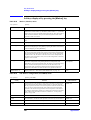
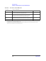
Functions of hardkeys . . . . . . . . . . . . . . . . . . . . . . . . . . . . . . . . . . . . . . . . . . . . . . . . . . . . . . . . . . . . . . . . . 358
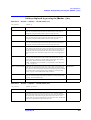
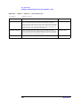
Softkeys displayed by pressing the [Meas] key . . . . . . . . . . . . . . . . . . . . . . . . . . . . . . . . . . . . . . . . . . . . . 361
Softkeys displayed by pressing the [Format] key . . . . . . . . . . . . . . . . . . . . . . . . . . . . . . . . . . . . . . . . . . . . 363
Softkeys displayed by pressing the [Display] key . . . . . . . . . . . . . . . . . . . . . . . . . . . . . . . . . . . . . . . . . . . 364
Softkeys displayed by pressing the [Scale Ref] key . . . . . . . . . . . . . . . . . . . . . . . . . . . . . . . . . . . . . . . . . . 371
Softkeys displayed by pressing the [Bw/Avg] key . . . . . . . . . . . . . . . . . . . . . . . . . . . . . . . . . . . . . . . . . . . 374
15
Contents
Softkeys displayed by pressing the [Cal] key. . . . . . . . . . . . . . . . . . . . . . . . . . . . . . . . . . . . . . . . . . . . . . .
Softkeys displayed by pressing the [Sweep] key . . . . . . . . . . . . . . . . . . . . . . . . . . . . . . . . . . . . . . . . . . . .
Softkeys displayed by pressing the [Source] key . . . . . . . . . . . . . . . . . . . . . . . . . . . . . . . . . . . . . . . . . . . .
Softkeys displayed by pressing the [Trigger] key . . . . . . . . . . . . . . . . . . . . . . . . . . . . . . . . . . . . . . . . . . .
Softkeys displayed by pressing the [Marker] key . . . . . . . . . . . . . . . . . . . . . . . . . . . . . . . . . . . . . . . . . . .
Softkeys displayed by pressing the [Marker→] key . . . . . . . . . . . . . . . . . . . . . . . . . . . . . . . . . . . . . . . . .
Softkeys displayed by pressing the [Search] key . . . . . . . . . . . . . . . . . . . . . . . . . . . . . . . . . . . . . . . . . . . .
Softkeys displayed by pressing the [Utility] key . . . . . . . . . . . . . . . . . . . . . . . . . . . . . . . . . . . . . . . . . . . .
Softkeys displayed by pressing the [System] key . . . . . . . . . . . . . . . . . . . . . . . . . . . . . . . . . . . . . . . . . . .
Softkeys displayed by pressing the [Local] key . . . . . . . . . . . . . . . . . . . . . . . . . . . . . . . . . . . . . . . . . . . . .
Softkeys displayed by pressing the [Copy] key . . . . . . . . . . . . . . . . . . . . . . . . . . . . . . . . . . . . . . . . . . . . .
Softkeys displayed by pressing the [Save] key . . . . . . . . . . . . . . . . . . . . . . . . . . . . . . . . . . . . . . . . . . . . .
Softkeys displayed by pressing the [Recall] key . . . . . . . . . . . . . . . . . . . . . . . . . . . . . . . . . . . . . . . . . . . .
376
381
386
388
390
393
395
400
402
413
415
419
425
C. Error messages
Error Messages (alphabetical order). . . . . . . . . . . . . . . . . . . . . . . . . . . . . . . . . . . . . . . . . . . . . . . . . . . . . . 428
16
1
Installation
This chapter contains installation and setup instructions for the Agilent 4294A Precision
Impedance Analyzer. For information on connecting test accessories such as a test fixture,
adapter, probe, or measurement cable, refer to Chapter 4 , “Preparation of Measurement
Accessories.”
17
Installation
Incoming Inspection
Incoming Inspection
WARNING
To avoid hazardous electrical shock, do not turn on the Agilent 4294A if there are
signs of shipping damage to any portion of the outer enclosure (for example, covers,
panel, or display).
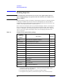
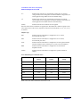
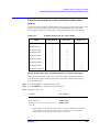
Check the shipping container for damage. If the shipping container or cushioning material
is damaged, it should be kept until the contents of the shipment have been checked for
completeness and the Agilent 4294A has been checked mechanically and electrically. The
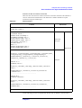
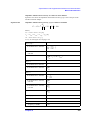
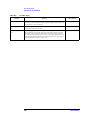
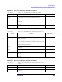
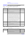
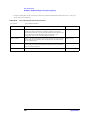
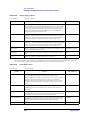
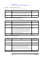
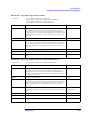
contents of the shipment should be as listed in Table 1-1.
If the contents are incomplete, there is any mechanical damage or defect, or the analyzer's
power-on self-test fails, contact the nearest Agilent Technologies office. If the shipping
container is damaged or the cushioning material shows signs of unusual stress, notify the
carrier as well as the Agilent Technologies office. Save the shipping materials for the
carrier's inspection.
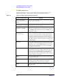
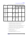
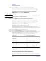
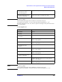
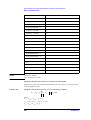
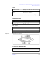
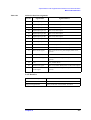
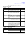
Table 1-1
Contents of the Agilent 4294A package
Agilent
product/part
number1
Description
Quantity
4294A
4294A Precision Impedance Analyzer
1
04294-900x0
Operation Manual (this guide)
1
04294-900x1
Programming Manual
1
E2083-90005
HP Instrument BASIC User's Handbook
1
04294-901x0
Service Manual2
1
04294-180x0
Sample Program Disk (3.5-inch floppy disk)
1
04294-61001
100 Ω resistor (for adapter setup)
1
C3757-60401
Mini-DIN keyboard3
1
8120-4753
Power Cable
1
1250-1859
BNC Adapter4
1
5062-3991
Handle Kit5
1
5062-3979
Rack Mount Kit6
1
5062-3985
Rack Mount & Handle Kit7
1
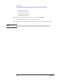
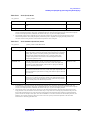
1. The number of “x” in the part number of each manual or sample program disk,
0 for the first edition, is incremented by 1 each time a revision is made. The latest edition comes with the product.
2. Not supplied unless the product is purchased with Option 0BW.
3. Not supplied if the product is purchased with Option 1A2 (without keyboard).
18
Chapter 1
Installation
Incoming Inspection
4. Not supplied unless the product is purchased with option ID5 (High Stability
Frequency Reference)
5. Not supplied unless the product is purchased with Option 1CN.
6. Not supplied unless the product is purchased with option 1CM.
7. Not supplied unless the product is purchased with Option 1CP.
Chapter 1
19
Installation
Precautions to Take Before Setting Up the Power Supply
Precautions to Take Before Setting Up the Power Supply
Before supplying electrical power to the Agilent 4294A, make sure that the correct fuse is
selected. Be sure to use a power source that meets the specifications listed later in this
section.
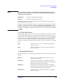
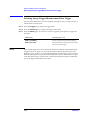
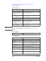
Setting Up and Replacing the Fuse
The Agilent 4294A requires the following fuse:
UL/CSA type, time delay, 5 A 250 Vac (Agilent part number 2110-0030)
Spare fuses are available from your nearest Agilent Technologies Sales and Service Office.
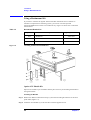
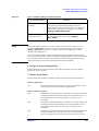
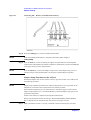
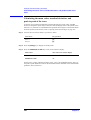
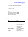
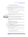
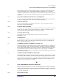
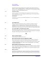
You can check and replace the fuse by dismounting the fuse folder shown in Figure 1-1. To
dismount the fuse holder, first disconnect the power cable, then use a flat-blade
screwdriver or similar tool to push the portion marked “a” in Figure 1-1 upward so that the
holder surface rises up a little, and finally pull off the holder.
Figure 1-1
Fuse holder and power inlet
Power Source Requirements
The Agilent 4294A requires a power source that meets the following specifications.
Voltage:
90 to 132 Vac or 198 to 264 Vac (auto select)
Frequency:
47 to 63 Hz
Power consumption:
300 VA (max)
20
Chapter 1
Installation
Power Cable
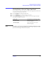
Power Cable
In accordance with international safety standards, the Agilent 4294A uses a three-wire
power cable. When connected to an appropriate ac power outlet, this cable grounds the
instrument frame through one of the three wires.
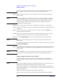
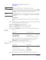
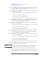
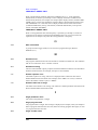
The type of power cable shipped with each instrument depends on the country of
destination. Refer to Figure 1-2 for the part numbers of the power cables available.
WARNING
For protection against electrical shock, the power cable grounding prong must not be
removed.
The power plug must be plugged into an outlet that provides an appropriate
receptacle for the ground connection.
Chapter 1
21
Installation
Power Cable
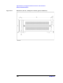
Figure 1-2
Alternative Power Cable Options
22
Chapter 1
Installation
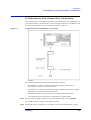
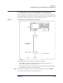
Connecting the BNC Adapter (for Option 1D5 Only)
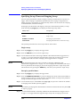
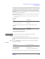
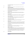
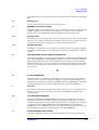
Connecting the BNC Adapter (for Option 1D5 Only)
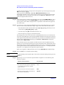
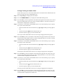
When Option 1D5 is installed, connect the BNC cable that comes with this option between
the REF OVEN and EXT REF INPUT connectors on the rear panel of the Agilent 4294A.
Option 1D5 makes the frequency of the Agilent 4294A’s test signal both more stable and
more accurate.
Figure 1-3
Connecting the BNC Adapter (for Option 1D5 Only)
Chapter 1
23
Installation
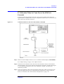
Using the LAN Port
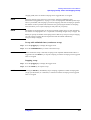
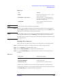
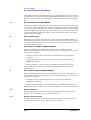
Using the LAN Port
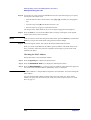
You can connect the Agilent 4294A to a local area network by using the RJ-45J UTP
(Unshielded Twisted Pair) LAN connector provided on the rear panel.
Step 1. To connect the 4294A to a LAN, securely insert the LAN cable into the LAN port.
Step 2. For the 4294A to communicate over a LAN, you must set up the network connection as
described in the section “Using LAN” in the “Programming Manual.”
Figure 1-4
Using the LAN Port
24
Chapter 1
Installation
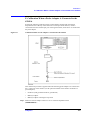
Connecting the Supplied Keyboard
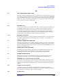
Connecting the Supplied Keyboard1
Step 1. Insert the cable of the supplied Mini-DIN keyboard into the keyboard connector on the rear
panel.
Step 2. Set the keyboard in a comfortable position.
NOTE
Do not put anything on the keyboard. Doing so can cause an error during the power-on
self-test.
Figure 1-5
Connecting the Supplied Keyboard
1. The Agilent 4294A does not come with a keyboard if it is purchased with Option 1A2 (without keyboard).
Chapter 1
25
Installation
Using a Rackmount Kit
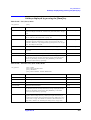
Using a Rackmount Kit
If you want to combine the Agilent 4294A with other instruments and a controller to
assemble a comprehensive measuring system, you can use one of the optional
rackmount/handle kits to install it in an efficient way. Figure 1-6 shows how to install the
rackmount kit.
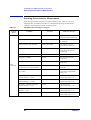
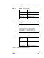
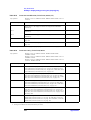
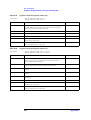
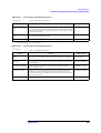
Table 1-2
Rackmount/Handle Kits
Option ID
Figure 1-6
Description
Agilent part number
1CN
Handle Kit
5062-3991
1CM
Rackmount Kit
5062-3979
1CP
Rackmount & Handle Kit
5062-3985
Installing the Rackmount/Handle Kit
Option 1CN Handle Kit
Option 1CN includes a pair of handles and the parts necessary for attaching the handles to
the Agilent 4294A.
Installing the Handles
Step 1. Remove the adhesive-backed trim strips (1) from the left and right side faces of the front
panel frame (Figure 1-6).
Step 2. Attach the front handles (3) to the side faces with the supplied screws.
26
Chapter 1
Installation
Using a Rackmount Kit
Step 3. Attach the trim strips (4) to the handles.
Option 1CM Rackmount Kit
Option 1CM includes a pair of flanges and the parts necessary for attaching them to the
Agilent 4294A. With this option, you can mount the 4294A on an equipment rack with
482.6 mm (19 inch) horizontal spacing.
Mounting the Agilent 4294A on a Rack
Step 1. Remove the adhesive-backed trim strips (1) from the left and right side faces of the front
panel frame (Figure 1-6 on page 26).
Step 2. Attach the flanges (2) to the side faces with the supplied screws.
Step 3. Remove all four legs from the bottom face by pulling up the tabs and sliding the legs out in
the direction indicated by the arrows.
Step 4. Mount the 4294A on the rack.
Option 1CP Rackmount & Handle Kit
Option 1CP includes two flanges and two handles along with their attachments.
Mounting the Agilent 4294A on a Rack (with Handles)
Step 1. Remove the adhesive-backed trim strips (1) from the left and right side faces of the front
panel frame (Figure 1-6 on page 26).
Step 2. Attach the handles (3) and flanges (5) to the side faces with the supplied screws.
Step 3. Remove all four legs from the bottom face by pulling up the tabs and sliding the legs out in
the direction indicated by the arrows.
Step 4. Mount the 4294A on the rack.
Chapter 1
27
Installation
Environmental Requirements
Environmental Requirements
The Agilent 4294A is designed to operate under the following environmental conditions
(with the floppy disk drive operational). For more information, refer to Chapter 10 ,
“Specifications and Supplemental Performance Characteristics,” on page 323.
NOTE
Temperature:
10°C to 40°C
Humidity:
15% to 80% (relative humidity)
The Agilent 4294A must be protected from temperature extremes that could cause
condensation within the instrument.
Ventilation Requirements
To ensure adequate ventilation, make sure that there is adequate clearance of at least
180 mm behind the unit and 60 mm at each side.
Instructions for Cleaning
To prevent electrical shock, disconnect the Agilent 4294A's power cable from the power
outlet before cleaning.
To clean the exterior of the Agilent 4294A, gently wipe the surfaces with a dry cloth or a
soft cloth that is soaked with water and wrung tightly. Do not attempt to clean the 4294A
internally.
28
Chapter 1
2
Learning Operation Basics
This chapter guides you through a tour of the basic measurement functions of the Agilent
4294A Precision Impedance Analyzer. If you are new to the Agilent 4294A, this tutorial
should help you get familiar with the instrument.
29
Learning Operation Basics
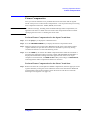
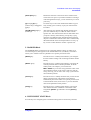
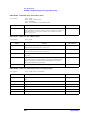
Required Equipment
Required Equipment
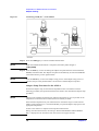
To perform all of the steps in this tour, you must have the following equipment:
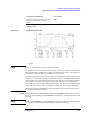
Figure 2-1
•
Agilent 4294A Precision Impedance Analyzer (1 unit)
•
16047E Text Fixture for Lead Components (1 piece)
•
DUT: Capacitor with lead wires having self-resonance frequency of 100 MHz or lower,
such as a 0.1 µF ceramic capacitor (1 piece)
Required Equipment
30
Chapter 2
Learning Operation Basics
Preparing for a Measurement
Preparing for a Measurement
Prepare the Agilent 4294A for measurement by taking the following steps. This procedure
assumes that the Agilent 4294A has been correctly installed and set up as described in
Chapter 1 , “Installation,” on page 17.
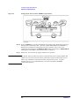
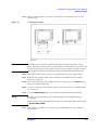
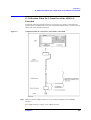
Connect the Agilent 16047E Test Fixture
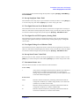
Connect the Agilent 4294A to the Agilent 16047E Test Fixture for Lead Components.
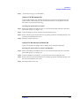
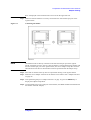
Step 1. Attach the 16047E test fixture to the test connectors on the front panel of the Agilent
4294A by gradually coupling the four BNC connectors and fastening screws of the fixture
with the test connectors and accessory mounting holes of the instrument until they are in
complete contact.
Step 2. Fasten two of the four BNC connectors to the corresponding test connectors by gradually
turning the BNC connectors' rotation levers until each pair of connectors is securely
connected. Be sure to align the grooves on both sides.
Step 3. Simultaneously turn the fixture's two fastening screws clockwise so that the fixture is
secured to the instrument.
Step 4. Finally, secure the remaining two BNC connectors of the fixture by turning their rotation
levers clockwise.
Figure 2-2
Connecting the Agilent 16047E Test Fixture
NOTE
Reverse the above procedure when removing the Agilent 16047E Test Fixture.
Chapter 2
31
Learning Operation Basics
Preparing for a Measurement
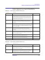
Turn ON the Power
Press the power switch to turn on the power to the Agilent 4294A.
The Agilent 4294A performs a power-on self-test. During the self-test, the model name,
firmware revision number/date, options, copyright notice, and other information appear on
the LCD. When the self-test is completed, the measurement screen appears on the LCD.
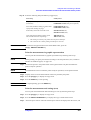
Set the Adapter Type to “NONE”
Use the keystroke sequence [Cal] - ADAPTER [ ] - NONE to configure the Agilent 4294A
to operate without an adapter.
This option must be selected when the Agilent 4294A is connected to a direct-coupling
type test fixture such as the Agilent 16047E. With the adapter type set to “NONE,” the
Instrument Status area on the measurement screen does not display the “EX1,” “EX2,”
“7mm,” and “PRB” indicators.
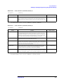
NOTE
When you use the Agilent 4294A for actual applications, you may want to use an adapter
such as a 7-mm conversion adapter (terminal adapter), cable, or probe. To do so, you must
specify the appropriate adapter type and then perform a calibration procedure called
“Adapter Setup,” in which you calibrate the Agilent 4294A for the connected adapter by
measuring a specific calibration standard. However, because this example uses the Agilent
16047E, which is a direct-coupling fixture that does not require an adapter, you need not
perform the “Adapter Setup” procedure in this tour.
For the Agilent 4294A to perform measurement, you must select the appropriate
adapter type option. Whenever you start a new measurement session, you should
check the indicator (“EX1,” “EX2,” “7mm,” “PRB,” or blank) shown in the
Instrument Status area to confirm that the correct adapter type is selected. Do not
forget to check the adapter type, particularly if you frequently reconnect the Agilent
4294A to a number of alternative adapters (including a 7-mm conversion adapter,
probe, cable, test fixture, and so on).
32
Chapter 2
Learning Operation Basics
Specifying Measurement Conditions
Specifying Measurement Conditions
Next, you need to specify how your Agilent 4294A should perform measurement.
NOTE
Through this procedure, you will configure parameters that apply to both Traces A and B.
You can set each parameter without specifying the active trace or checking its current
setting.
Initialize the Agilent 4294A to the Preset State
Press the [Preset] key to initialize the Agilent 4294A.
This puts the Agilent 4294A into its preset state.
NOTE
If you turn on the Agilent 4294A with a power-on setting file residing on the flash memory
(nonvolatile memory disk) or on a floppy disk inserted in the floppy disk drive, the file is
automatically loaded, and the settings contained in the file are restored. Initializing the
Agilent 4294A to its preset state ensures that no specific settings are inherited from the last
measurement session. Therefore, you should initialize the Agilent 4294A by pressing the
[Preset] key whenever you are configuring it for a new measurement session, regardless of
whether you turned the instrument off and back on after the previous session.
Note that initializing the Agilent 4294A with the [Preset] key does not affect which type of
adapter the instrument is configured to use. Once you have set the adapter type, the setting
is retained until you select another adapter type.
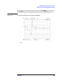
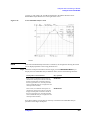
Select |Z|-θ as the Measurement Parameter
To select the measurement parameter, follow these steps:
Step 1. Press the [Meas] key to display the Measurement Parameter menu.
Step 2. Make sure that the |Z|-θ key is selected (this key is selected by default in the preset state).
With the |Z|-θ key selected, Trace A reflects the absolute impedance value while Trace B
reflects the impedance phase.
Select Frequency as the Sweep Parameter
Step 1. Press the [Sweep] key to display the Sweep menu.
Step 2. Check the PARAMETER [ ] softkey label to confirm that “FREQ” (frequency sweep) is
shown between the brackets [ ] (this setting is selected by default in the preset state).
NOTE
The Sweep Parameter menu, which is not used in this tour, allows you to change the sweep
parameter. You can access this menu by pressing the PARAMETER [ ] key.
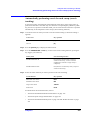
Select Logarithmic Sweep as the Sweep Type
Step 1. From the Sweep menu, select TYPE [ ] to display the Sweep Type menu.
Chapter 2
33
Learning Operation Basics
Specifying Measurement Conditions
Step 2. Press the LOG key to select Log (logarithmic) sweep.
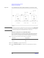
Set the Sweep Start Value to 100 Hz
Step 1. Press the [Start] key. The current setting of the sweep start value appears in the Parameter
Setting field in the upper-left area of the screen.
Step 2. Type “100” into the Parameter Setting field using these ENTRY block keys: [1][0][0].
Step 3. Specify that the value does not take any unit by pressing the [×1] key in the ENTRY block.
This puts your entry into effect.
Set the Sweep Stop Value to 100 MHz
Step 1. Press the [Stop] key. The current setting of the sweep stop value appears in the
Measurement Parameter field in the upper-left area of the screen.
Step 2. Type “100” into the Parameter Setting field using these ENTRY block keys: [1][0][0].
Step 3. Suffix your entry with “M” (mega) by pressing the [M/m] key in the ENTRY block. This
puts your entry into effect.
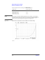
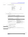
Set the Measurement Bandwidth to 2
Step 1. Press the [Bw/Avg] key to display the Measurement Bandwidth/Averaging menu.
Step 2. Press the BANDWIDTH [ ] key to display the Measurement Bandwidth Setting menu.
Step 3. Set the measurement bandwidth to 2 by pressing the 2 key.
34
Chapter 2
Learning Operation Basics
Fixture Compensation
Fixture Compensation
Next, you need to eliminate errors produced between the test fixture and the Agilent
4294A. This process is called “fixture compensation.” You can perform the process using
three compensation functions: OPEN, SHORT, and LOAD.
NOTE
All calibration settings, including those established through fixture compensation, are
applied to both Traces A and B. You can execute each compensation function without
specifying the active trace or checking the current state.
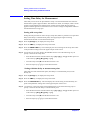
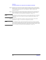
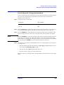
Perform Fixture Compensation for the Open Circuit State
Step 1. Press the [Cal] key to display the Calibration menu.
Step 2. Press the FIXTURE COMPEN key to display the Fixture Compensation menu.
Step 3. Make sure that the two test electrodes, HIGH and LOW, of the connected text fixture
(Agilent 16047E) are open. Be sure to fix the two electrodes in position by turning
clockwise the fixture’s two electrode fastening screws.
Step 4. Press the OPEN key to measure the OPEN compensation data. While the instrument is
measuring the compensation data, a message “WAIT--MEASURING STANDARD” is
displayed in the Parameter Setting field in the upper-left area of the screen. Upon
completion of measurement, the OPEN on OFF softkey label changes to OPEN ON off,
indicating that the OPEN compensation function is turned on.
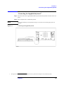
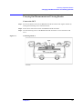
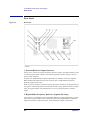
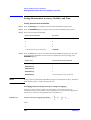
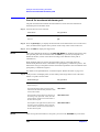
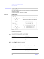
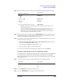
Perform Fixture Compensation for the Short Circuit State
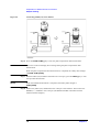
Step 1. Remove the short bar (a metal plate for SHORT compensation) from the upper part of the
Agilent 16047E by loosing the screws and then fit the short bar between the HIGH and
LOW terminals of the Agilent 16047E. Secure the short bar with the two electrode
fastening screws (Figure 2-3 on page 36).
Chapter 2
35
Learning Operation Basics
Fixture Compensation
Figure 2-3
Setting Up the Test Circuit for SHORT Compensation
Step 2. Press the SHORT key to measure the SHORT compensation data. While the instrument is
measuring the compensation data, a message “WAIT--MEASURING STANDARD” is
displayed in the Parameter Setting field in the upper-left area of the screen. Upon
completion of measurement, the SHORT on OFF softkey label changes to SHORT ON off,
indicating that the SHORT compensation function is turned on.
Step 3. Remove the short bar from the Agilent 16047E's test electrodes.
NOTE
The Agilent 4294A provides three fixture compensation functions: OPEN, SHORT, and
LOAD. You can turn on/off each of these compensation functions individually and use
them in any combination to perform the fixture compensation process. In typical
measurement use, it is recommended that you execute the OPEN and SHORT
compensation functions.
36
Chapter 2
Learning Operation Basics
Carrying Out Measurement and Viewing Results
Carrying Out Measurement and Viewing Results
Connect the DUT
Step 1. Increase the distance between the HIGH and LOW electrodes of the Agilent 16047E by
turning their fastening screws counterclockwise.
Step 2. Fit the DUT's lead wires between the HIGH and LOW electrodes.
Step 3. Turn the fastening screws of the HIGH and LOW electrodes to secure the DUT's lead
wires.
Figure 2-4
Connecting the DUT
Chapter 2
37
Learning Operation Basics
Carrying Out Measurement and Viewing Results
Figure 2-5
Measurement results displayed just after connecting the DUT
Apply the Logarithmic Format to the Vertical Axis for |Z|
Step 1. Make sure that Trace A is selected as the active trace (Trace A is active by default in the
preset state).
Step 2. Press the [Format] key to display the Display Format menu.
Step 3. Press the LOG key to make the graph's vertical axis logarithmic.
Apply the Linear Format to the Vertical Axis for θ
Step 1. Press the [B] key to activate Trace B.
Step 2. Make sure that the graph's vertical axis is in the linear format with the LIN key selected
(this setting is selected by default in the preset state).
38
Chapter 2
Learning Operation Basics
Carrying Out Measurement and Viewing Results
Figure 2-6
Result of Applying the Logarithmic Format to the Graph
Display the Measured |Z| and θ Values in Parallel
Step 1. Press the [Display] key to display the Display menu.
Step 2. Press the SPLIT on OFF key to split the screen into upper and lower halves (the key label
should change to SPLIT ON off).
Chapter 2
39
Learning Operation Basics
Carrying Out Measurement and Viewing Results
Figure 2-7
Displaying Traces A and B in Parallel
NOTE
You do not need to check which trace is active when you split the screen because this
setting is applied to both Traces A and B.
Auto-scale the |Z| Trace
Step 1. Press the [A] key to activate Trace A.
Step 2. Press the [Scale Ref] key to display the Scale Reference menu.
Step 3. Press the AUTO SCALE key to auto-scale the trace for |Z|.
Auto-scale the θ Trace
Step 1. Press the [B] key to activate Trace B.
Step 2. Press the AUTO SCALE key to auto-scale the trace for θ.
40
Chapter 2
Learning Operation Basics
Carrying Out Measurement and Viewing Results
Figure 2-8
Results of Auto-scaling
Chapter 2
41
Learning Operation Basics
Results of Analysis
Results of Analysis
Determine the Self-resonance Frequency and Resonant Impedance
Step 1. Press the [A] key to activate Trace A.
Step 2. Press the [Search] key to display the Search menu. The main marker (a trace marker
identified by number 0) appears in the center of the graph.
Step 3. Press the SEARCH TRK on OFF key to turn on the search tracking function (the key label
should change to SEARCH TRK ON off). When this function is enabled, the instrument
performs a search action upon completion of each sweep cycle.
Step 4. Press the MIN key to move the main marker to the minimum |Z| value. Since the search
tracking function is enabled, the instrument detects and moves the main marker to the
minimum |Z| value each time it has completed one sweep cycle.
You can determine the self-resonance frequency and resonant impedance by reading the
sweep parameter (frequency) and measurement parameter values indicated by the main
marker that appears in the upper-left area of the graph for Trace A. In the example shown
in Figure 2-9, the DUT exhibits its self-resonance frequency and resonant impedance at
approximately 5.13 MHz and 155 mΩ, respectively.
Figure 2-9
Result of Searching for the Self-Resonance Frequency (with the Search Tracking
Function On)
42
Chapter 2
3
Front/Rear Panel and LCD Display
This chapter covers the features of the front and rear panels of the Agilent 4294A. It
contains illustrations and descriptions of the front panel features, the LCD display and its
labels, and the rear panel connectors.
43
Front/Rear Panel and LCD Display
Front Panel
Front Panel
The front panel of the Agilent 4294A provides several blocks of hardkeys and an LCD
display with a series of softkeys along its right-hand edge. Also, there are a number of test
connectors and a power switch beneath the LCD display. Figure 3-1 shows the front panel
of the Agilent 4294A.
Figure 3-1
Front Panel of the Agilent 4294A
Hardkeys
The hardkeys are 46 physical keys located on the upper-right part of the front panel; they
are divided into six functionally classified blocks (#1 to #6 in Figure 3-1). Each hardkey is
labeled with text that describes its function. The eight keys laid out vertically along the
right-hand edge of the LCD display are called “softkeys” to distinguish them from the
hardkeys. Note that the term “hardkey” refers to all of the controls within each of the six
key blocks, including the circular-shaped rotary knob (❍) in the Entry block.
A hardkey either directly controls the functions of the Agilent 4294A, provides access to
softkey menus, or both.
44
Chapter 3
Front/Rear Panel and LCD Display
Front Panel
NOTE
As a typographic convention to distinguish between hardkeys and softkeys, this
manual uses a pair of brackets ([ ]) to enclose hardkey labels while showing softkey
labels without enclosing them.
[Hardkey] key
Indicates a hardkey labeled “Hardkey.”
Softkey key
Indicates a softkey labeled “Softkey.”
Note that descriptive text in this manual sometimes only indicates key labels without
following them by the word “key.”
When several keys are separated by a hyphen (-), press them in the sequence indicated. For
example, you should use the keystroke sequence [Scale Ref] - AUTO SCALE to enable
automatic scale adjustment. As an exception, numeric keys may appear without a hyphen
in between; for example, the keystroke sequence to enter a value of 100 may be expressed
as [1][0][0].
1. ACTIVE TRACE block
With the Agilent 4294A, you can view two traces (waveforms) for each sweep cycle: Trace
A and Trace B. Some parameters, such as the sweep range, apply to both traces, while
other parameters can be separately configured for each trace. You can use the [A] or [B] key
in the Active Trace block to choose between Traces A and B. Once you have activated
either trace, you can configure measurement conditions and perform analysis on that
“active” trace. When you set measurement conditions, be aware of which trace is currently
active.
[A] key
Activates Trace A so you can set conditions and perform
analysis on Trace A.
[B] key
Activates Trace B so you can set conditions and perform
analysis on Trace B.
2. MEASUREMENT Block
This block provides keys for configuring all measurement conditions except the test signal
settings.
[Meas] key
Provides access to a softkey menu that lets you select
measurement parameters.
[Format] key
Provides access to softkey menus that let you select the
data display format (graph axis format) and set up the phase
display unit and phase expansion feature.
[Display] key
Provides access to softkey menus that let you configure
general display options (except the display format and scale
setting) and perform equivalent circuit analysis.
[Scale Ref] key
Provides access to a softkey menu that lets you configure
graph scale settings.
Chapter 3
45
Front/Rear Panel and LCD Display
Front Panel
[Bw/Avg] key
Provides access to a softkey menu that lets you configure
the bandwidth and averaging settings.
[Cal] key
Provides access to a softkey menu that lets you set up the
calibration feature.
3. STIMULUS Block
This block provides keys for configuring the test signal parameters.
[Sweep] key
Provides access to a softkey menu that lets you configure
the sweep settings for the test signals.
[Source] key
Provides access to a softkey menu that lets you configure
the frequency (CW frequency), test signal level, and dc bias
conditions. When you are setting a sweep parameter, you
can use the [Start], [Stop], [Center], and [Span] keys to set
the sweep range.
[Trigger] key
Provides access to a softkey menu that lets you set up the
trigger system.
[Start] key
Lets you specify the value at which to start the sweep.
[Stop] key
Lets you specify the value at which to stop (finish) the
sweep.
[Center] key
Lets you specify the sweep center value.
[Span] key
Lets you specify the sweep span value.
4. ENTRY Block
Provides keys for entering numeric values and text strings. To configure a parameter, first
press the hardkey or softkey associated with the parameter to put the instrument into entry
mode, in which it can accept your entry with the name and current value of the parameter
shown in the upper-left area of the LCD display, and then use these keys to enter the
desired value.
❍ (rotary knob)
You can adjust the current setting by turning this knob. This
method immediately updates the parameter value without
requiring you to press a unit key. When working with a
particular configuration item, you can also use the rotary
knob to move the cursor horizontally.
[↑] and [↓] keys
The step keys allow you to increment or decrement the
current setting. This method immediately updates the
parameter value without requiring you to press a unit key.
(step keys)
[Entry Off] key
46
This key switches the instrument from entry mode to
normal operation mode with the name and current setting
of the parameter no longer shown in the upper-left area of
the LCD display.
Chapter 3
Front/Rear Panel and LCD Display
Front Panel
[Back Space] key
Deletes the character to the left of cursor and moves the
cursor back one space. If you make a mistake in entering a
value through numeric keys, you can use this key to correct
your entry.
[0] through [9] keys
Use these keys to enter each numeral that makes up your
entry. Finally, press a unit key to put your entered value
into effect.
(numeric keys) with [.] and
[-] keys
[G/n][M/µ][k/m][×1] keys
(unit keys)
After entering your desired value through numeric keys,
press one of the unit keys to suffix the value with the
specific unit. Your entered value does not take effect until
you press a unit key. Each unit key, except the [×1] key,
represents two different units, identifying them with their
respective initial letters. Which unit to use is automatically
determined based on the selected parameter. Use the [×1]
key to enter a value that does not take a specific unit.
5. MARKER Block
The MARKER block provides keys for configuring marker settings. A marker is an
inverted triangle (∇) that appears on the measurement trace (waveform). The marker
allows you to read the value of a parameter at a specific point on the trace.
[Marker] key
Provides access to a softkey menu that lets you configure
the basic marker settings such as turning on/off the marker
facility.
[Marker→] key
Provides access to a softkey menu that lets you assign the
currently marked value to another parameter. From the
softkey menu, for example, you can select the
MKR→START key to use the sweep parameter value at the
current marker position as the value at which to start the
sweep; this way, you can start a new sweep cycle from the
current marker position.
[Search] key
Provides access to a softkey menu that lets you activate the
marker search function. The marker search function
automatically moves the marker to a specific position (such
as the maximum value) on the trace so you can check the
value of the parameter at that position.
[Utility] key
Provides access to a softkey menu that lets you activate
other marker functions in addition to the marker value
assignment ([Marker→]) and marker search ([Search])
functions.
6. INSTRUMENT STATE Block
Provides keys for configuring basic instrument settings that are not directly related to
Chapter 3
47
Front/Rear Panel and LCD Display
Front Panel
measurement or analysis.
[System] key
Provides access to a softkey menu that lets you control and
manage the entire instrument. You can also set up the limit
line test function.
[Local] key
Pressing this key switches the Agilent 4294A from remote
mode (in which it is controlled by an external controller) to
local mode (in which it accepts keystrokes from its front
panel). While the instrument is in remote mode, the “Rmt”
LED above this key is lit. This key also provides access to a
softkey menu that lets you configure the GP-IB and LAN
settings.
[Preset] key
Initializes the Agilent 4294A to its preset state. No softkey
menu is displayed after you put the instrument into the
preset state by pressing this key, but you can display a
softkey menu by pressing one of the hardkeys associated
with softkey menus.
[Copy] key
Provides access to a softkey menu that lets you control how
to output the screen contents to the printer.
[Save] key
Provides access to a softkey menu that lets you save such
information as the current settings, measurement data, and
screen contents to the storage device of the Agilent 4294A.
[Recall] key
Provides access to a softkey menu that lets you recall (load)
a state file from the storage device of the Agilent 4294A to
restore the settings and measurement data stored in the state
file.
7. Softkeys
The softkeys are eight keys located along the right-hand edge of the LCD display. Pressing
a hardkey displays a menu of labels that define the functions of the softkeys. For more
information on softkey labels, refer to “5. Softkey Label Area” on page 54.
8. Color LCD Display
Displays nearly all information necessary for using the Agilent 4294A, including
measurement results (trace data), instrument status, analysis results, and softkey labels.
9. Power Switch
Turns on/off the power to the instrument. When you turn on the Agilent 4294A, it is
initialized to its power-on defaults, with no softkey menu shown on the screen. From this
state, you can display a softkey menu by pressing a specific hardkey. Note that if you turn
on the instrument with a power-on setting file (AUTOREC.STA) residing on the flash
memory (nonvolatile memory disk) or on a floppy disk inserted in the floppy disk drive,
the file is automatically loaded, and the settings contained in the file are restored.
48
Chapter 3
Front/Rear Panel and LCD Display
Front Panel
10. UNKNOWN Terminals
These connectors let you connect the instrument with a device under test (DUT) via test
accessories (such as an adapter, test fixture, or cable). These accessories adopt a
four-terminal pair design, thereby enabling more accurate and wider-range dynamic
measurements. Each test connector has a pair of holes for securing the test accessory to the
instrument.
INSTALLATION CATEGORY I
CAUTION
To prevent failure, do not apply dc voltage or current to the UNKNOWN terminal. Special
care must be taken with capacitors since they may be charged. Be sure to connect the DUT
to the UNKNOWN terminal (or test fixture) only after discharging them sufficiently.
11. Built-in 3.5 Inch Floppy Disk Drive
Allows you to store and retrieve such data as measurement data, instrument settings, screen
contents, and HP Instrument BASIC programs. This drive uses a 3.5-inch, MS-DOS format
floppy disk of 1.44 MB capacity.
Chapter 3
49
Front/Rear Panel and LCD Display
Rear Panel
Rear Panel
Figure 3-2
Rear Panel
1. External Reference Input Connector
Allows you to connect an external frequency reference signal to the Agilent 4294A so that
its internal signal is phase locked to the external frequency reference signal to achieve a
more accurate frequency.
If Option 1D5 (High Stability Frequency Reference) is installed, connect the supplied
BNC(m)-BNC(m) adapter between this connector and “2. High Stability Frequency
Reference (Option 1D5 Only)”.
When an external frequency reference signal is input to this connector, the Agilent 4294A's
test signal is automatically phase locked to that reference signal. When the reference signal
stops, the Agilent 4294A will automatically revert to its internal frequency reference
signal.
2. High Stability Frequency Reference (Option 1D5 Only)
This connector is intended for Option 1D5 (High Stability Frequency Reference) to output
the reference signal. If Option 1D5 is installed, connect the supplied BNC(m)-BNC(m)
adapter between this connector and Åu1. External Reference Input ConnectorÅv.
50
Chapter 3
Front/Rear Panel and LCD Display
Rear Panel
3. External Trigger Input
Allows you to input a TTL-compatible signal to trigger the execution of measurement.
When the signal shows a rising or falling edge between the LOW and HIGH states, a
measurement cycle is triggered. Before you can trigger measurement by inputting a signal
through this connector, you have to specify that the trigger signal be input from an external
trigger source (via the external trigger input). To do so, use the keystrokes: [Trigger] SOURCE [ ] - EXTERNAL. For more information on the input signal conditions specific to
this connector, refer to Chapter 10 , “Specifications and Supplemental Performance
Characteristics,” on page 323.
4. LAN Port
Allows you to connect the Agilent 4294A with a local area network (LAN). The “Tx”
(transmit) LED located on the right-hand side of the LAN port is lit while the Agilent
4294A is outputting data over the local area network. For more information on working
with a local area network, refer to the Programming Manual.
5. Internal Reference Output
Connects to the external reference input terminal of another instrument to phase lock it to
the Agilent 4294A.
6. External Program RUN/CONT Input
Allows you to input a TTL-compatible signal that triggers the RUN or CONTINUE
command for an HP Instrument BASIC program. When the signal shows a rising or falling
edge between the LOW and HIGH states, then the command is triggered. For more
information on the input signal conditions specific to this connector, refer to Chapter 10 ,
“Specifications and Supplemental Performance Characteristics,” on page 323.
7. 8-bit I/O Port
Provides a data communications interface with an external device such as a handler on a
production line. This port supports 4-bit data for input and 8-bit data for output.
8. Time Base Adjuster (for Option 1D5)
This adjuster is used to fine-tune the operating frequency of the Agilent 4294A when it is
equipped with Option 1D5 (High Stability Frequency Reference).
NOTE
This is intended for service center use only. Do not attempt to adjust the operating
frequency yourself.
9. Mini-DIN Keyboard Port
A PS/2 port intended for connecting a 101-key English keyboard. You can use a keyboard
to facilitate entry operations such as creating and executing HP Instrument Basic programs
or entering display titles.
NOTE
This port only supports a 101-key English keyboard with a PS/2 connector. Do not attempt
Chapter 3
51
Front/Rear Panel and LCD Display
Rear Panel
to use an unsupported keyboard.
10. 24-bit I/O Port
Provides a data communications interface with an external device such as a handler on a
production line. This port supports 8-bit data for input/output and 16-bit data for output.
11. Printer Port
A parallel port that connects to a printer. Connecting a supported printer allows you to print
out such data as measurement graphs and lists of measured values or settings. For a list of
supported printers, refer to “Print the measurement results and internal data with a printer”
on page 291.
12. External Monitor Terminal
Connects to an external color monitor. An external color monitor connected to this terminal
can display the same information as the Agilent 4294A's built-in LCD.
13. GPIB Connector
Allows you to connect the Agilent 4294A to any external controller or instrument that
supports GPIB (General Purpose Interface Bus). GPIB is useful when you want to
assemble an automatic measurement system by having the Agilent 4294A interact with a
controller and other instruments. For information on using GPIB to perform automatic
measurement, refer to “Programming Guide.”
14. Inlet (with a fuse box)
To use the Agilent 4294A, you must connect this inlet with the three-wire power cable that
comes with the Agilent 4294A. For more information, refer to Chapter 1, “Installation and
Setup.”
52
Chapter 3
Front/Rear Panel and LCD Display
Items Displayed on the LCD
Items Displayed on the LCD
Figure 3-3
Items displayed on the LCD (with split display mode off and full-screen mode on)
1. Measurement Parameter Fields
Each of these fields show the currently selected measurement parameters for either Trace
A or B.
2. Scale/Reference Fields
These fields show the current scale settings for Traces A and B.
3. Marker Measurement Parameter Value Fields
These fields show the measurement parameter values that correspond to the current marker
position for Traces A and B.
4. Menu Title Field
This field shows the name of the current softkey menu, which consists of up to 8 softkey
labels.
Chapter 3
53
Front/Rear Panel and LCD Display
Items Displayed on the LCD
5. Softkey Label Area
Shows the labels that are, in the current context, associated with the softkeys on the
right-hand side. Table 3-1 lists the types of softkey options and their functions.
Table 3-1
Types of softkey options and their functions
Type of softkey option
Function
Two or more softkey
labels joined with vertical
bars (|)
You can select one of these options. The currently selected
softkey label is underlined.
Softkey label immediately
followed by a “➤” symbol
Pressing the softkey displays a softkey sub-menu
associated with a specific function.
Softkey label followed by
“ON off” or “on OFF”
Pressing the corresponding softkey turns on/off the
function in a toggle fashion. The softkey label is followed
by “ON off” when the function is on and “on OFF” when
the function is off.
Softkey label immediately
followed by “[ ].”
The brackets ([ ]) enclose text that describes the current
setting of the associated function. If the function has two
alternative settings, pressing the softkey toggles between
the settings. If the function has three or more alternative
settings, the label is usually followed by “➤,” and pressing
the softkey displays a softkey sub-menu for selecting one
of those settings.
more n/m
This softkey label indicates that the softkey menu consists
of m pages, and that the nth page of the menu is currently
displayed. You can use the more n/m key to move to the
next page of the softkey menu (or to the first page if the
current page is the last one).
return
This softkey label is contained in a softkey sub-menu that is
displayed when you press a softkey followed by “➤.” You
can press the corresponding softkey to return to the main
menu, that is, the original softkey menu that had been
displayed before you accessed the current menu, as long as
the current menu is a sub-menu.
done
Select this softkey label to put your entry into effect and
return to the main menu.
yes
This softkey label appears when you are prompted to
confirm your entry before applying it. Pressing the
corresponding softkey puts your entry into effect.
cancel
Select this softkey label to cancel your entry and return to
the main menu.
54
Chapter 3
Front/Rear Panel and LCD Display
Items Displayed on the LCD
Table 3-1
Types of softkey options and their functions
Type of softkey option
Function
Softkey label for setting a
parameter1
Pressing the corresponding softkey displays the function's
current setting in the Parameter Setting field in the
upper-left part of the screen and allows you to change the
current setting with the Entry block keys (for example,
[Bw/Avg] - AVERATING FACTOR).
Softkey label for
executing a function1
Pressing the corresponding softkey immediately executes
the associated function (for example, [Marker] MKR→START).
1. These softkey labels are displayed without any special symbol.
NOTE
Some softkey labels combine two or more of the functions shown in Table 3-1. For
example, the EDIT LIST key, which can be accessed through the keystroke sequence
[Sweep] - EDIT LIST, both turns on “sweep list edit mode” and displays a softkey
sub-menu for editing the list.
Some of the softkey labels currently displayed may not be available depending on the
current context; such softkey labels are dimmed by displaying them at a lower contrast than
the other labels. When you choose the appropriate context by using another key, those
softkey labels will revert to the normal contrast and become available.
6. Sweep Parameter Reading Fields
These fields show the sweep parameter values that correspond to the current marker
position for Traces A and B.
7. Marker Status Fields
These fields provide textual representation of the current status of the marker facility.
Marker couple mode
Cpl
Indicates that the marker facility is currently in couple mode. In this
mode, changes to Traces A and B are synchronized.
Marker search track mode
Max
Indicates that the marker facility is currently in search track mode and
configured to detect the maximum value. The main marker moves to
the maximum value on the trace each time one sweep cycle is
completed.
Min
Indicates that the marker facility is currently in search track mode and
configured to detect the minimum value. The main marker moves to
the minimum value on the trace each time one sweep cycle is
completed.
Targ
Indicates that the marker facility is currently in search track mode and
configured to detect the specified target value. The main marker
moves to the target value on the trace each time one sweep cycle is
Chapter 3
55
Front/Rear Panel and LCD Display
Items Displayed on the LCD
completed.
Peak
Indicates that the marker facility is currently in search track mode and
configured to detect the peak value. The main marker moves to the
peak value on the trace each time one sweep cycle is completed.
∆ marker mode
∆Mkr
Indicates that the marker facility is currently in default ∆ marker
mode. In this mode, the ∆ marker keeps track of changes to the trace,
maintaining the same position in terms of the sweep parameter value.
Fxd∆
Indicates that the marker facility is currently in fixed ∆ marker mode.
In this mode, the ∆ marker is fixed at a certain point on the screen,
without reflecting any changes to the trace. It remains in the same
position in terms of both the sweep parameter and measurement
parameter values.
Trk∆
Indicates that the marker facility is currently in tracking ∆ marker
mode. In this mode, the ∆ marker appears in the same position as, and
moves synchronously with, the main marker,
8. Marker Statistics/Trace Bandwidth Analysis Fields
These fields show the marker statistics (average, standard deviation, and peak-to-peak
values) or the results of trace bandwidth analysis (bandwidth, center value, Q peak, ∆L,
and ∆R) for Traces A and B. When both features are enabled, they display the marker
statistics only.
9. Limit Line Test Fields
These fields show the results of limit line tests as either “PASS” or “FAIL.” By performing
a limit line test, you can determine whether the trace of measurement results falls within
your specified limit line.
10. HP Instrument Basic Status Indicator
Indicates the execution status of HP Instrument BASIC.
*
HP Instrument BASIC is currently executing a program or command.
You cannot execute an additional command.
_
HP Instrument BASIC has suspended the execution of a program. You
can resume the program using the CONTINUE command.
?
HP Instrument BASIC is waiting for a keystroke to continue the
execution of a program. You cannot execute an additional command.
(blank)
HP Instrument BASIC is not executing a program or command. You
can use commands other than the CONTINUE command.
11. dc Voltage/Current Bias Monitor Field
This field shows the monitor value (voltage or amperage) for the dc bias conditions that are
currently in effect. For this field to actually display the monitor value, you must apply dc
bias through the keystroke sequence [Source] - BIAS MENU - BIAS on OFF and then turn
56
Chapter 3
Front/Rear Panel and LCD Display
Items Displayed on the LCD
on the dc bias monitor feature through the keystroke sequence [Display] - BIAS MON [ ] VOLT/CURRENT.
12. Sweep Stop/Span Value Field
This field shows the sweep stop or span value that is currently in effect. Use the [Stop] key
to set the sweep stop value and the [Span] key to set the sweep span value.
13. Test Signal Current Level Monitor Field
This field shows the AC current level monitor value for the test signal that is currently in
effect. For this field to actually display the monitor value, you must turn on the test signal
level monitor feature through the keystroke sequence [Display] - OSC MON on OFF.
14. Test Signal Level/CW Frequency Setting Field
This field shows the test signal level setting for frequency sweep or the CW frequency
setting for test signal level sweep or dc bias sweep. Use the [Source] key to change the
current value.
15. Test Signal Voltage Level Monitor Field
This field shows the AC voltage level monitor value for the test signal that is currently in
effect. For this field to actually display the monitor value, you must turn on the test signal
level monitor feature through the keystroke sequence [Display] - OSC MON on OFF.
16. Sweep Start/Center Value Field
Shows the start or center value for the sweep settings that are currently in effect. Use the
[Start] key to set the sweep start value and the [Center] key to set the sweep center value.
17. Instrument Status Area
This area shows the status of various functions of the instrument.
Trace validity
*
After you have changed the measurement conditions, this indicator is
displayed until you update the measurement trace with the new
settings. To get a correct measurement trace, you must update the trace
so that this indicator disappears.
dc bias status
DCB
Indicates that the instrument is performing measurement under dc
voltage bias conditions (in variable voltage mode) or dc current bias
conditions (in variable current mode).
VC
Indicates that the instrument is performing measurement under dc
voltage bias conditions (in constant voltage mode).
IC
Indicates that the instrument is performing measurement under dc
current bias conditions (in constant current mode).
Chapter 3
57
Front/Rear Panel and LCD Display
Items Displayed on the LCD
V↓
Indicates that, because you specified dc voltage bias (in constant
voltage mode) with a setting that exceeds the defined voltage limit, the
actual applied voltage differs from the intended setting.
I↓
Indicates that, because you specified dc current bias (in constant
current mode) with a setting that exceeds the defined current limit, the
actual applied current differs from the intended setting.
(blank)
Indicates that dc bias conditions are not applied.
Note that when dc bias conditions are applied, the “DC BIAS ON” indicator appears in the
lower-right corner of the screen, regardless of which bias mode (DCB, VC, IC, V ↓, or I ↓)
is selected.
Adapter type
EX1
Indicates that the instrument is configured to use a 1-meter,
four-terminal pair cable.
EX2
Indicates that the instrument is configured to use a 2-meter,
four-terminal pair cable.
7mm
Indicates that the instrument is configured to use the Agilent 42942A
Terminal Adapter (four-terminal pair to 7-mm conversion adapter).
PRB
Indicates that the instrument is configured to use the 42941A
Impedance Probe.
(blank)
Indicates that the instrument is configured to operate without an
adapter.
User calibration/port extension status
User calibration
feature
Port extension
feature
Correction point
setting
CAL
ON
Fixed
Cal
ON
User-defined
POR
ON
Fixed
Por
ON
User-defined
CAP
ON
ON
Fixed
CaP
ON
ON
User-defined
(blank)
(Unknown)
Blank cells in the table indicate that the feature is off.
58
Chapter 3
Front/Rear Panel and LCD Display
Items Displayed on the LCD
Fixture compensation status
Fixture Compensation
feature
Correction point setting
CMP
ON
Fixed
Cmp
ON
User-defined
(blank)
(Unknown)
Blank cells in the table indicate that the feature is off.
NOTE
The user correction and fixture compensation features share the same correction point
settings. You cannot set correction points specific to a single feature.
Averaging status
Avg
Indicates that the sweep-to-sweep averaging feature is on.
(blank)
Indicates that the sweep-to-sweep averaging feature is off.
Averaging counter
(Positive integer)
When the sweep-to-sweep averaging feature is on, this counter
indicates how many times the current trace has been subjected to
sweep-to-sweep averaging. After you have started sweep-to-sweep
averaging, the counter shows “1” upon the 1st sweep cycle, “2” upon
the 2nd cycle, and so on until it reaches the maximum number of
averaging cycles. To view a trace subjected to your specified number
of averaging cycles, you must wait for the instrument to repeat the
sweep cycles until the counter reaches that number.
Data trace definition
D–M
Indicates that the currently displayed data trace represents the result of
subtracting the memory trace data from the measurement data.
D/M
Indicates that the currently displayed data trace represents the result of
dividing the measurement data by the memory trace data.
D%M
Indicates that the currently displayed data trace represents the result of
DATA – MEM
the following operation: ------------------------------------ × 100 [%] (where DATA is the
MEM
measurement data and MEM is the memory trace data).
NOTE
–O
Indicates that the currently displayed data trace represents the result of
subtracting the offset value from the measurement data.
(blank)
Indicates that the currently displayed data trace shows the exact
measurement data.
If “–O” appears below “D–M” or “D%M,” the data trace represents the result of
performing both operations on the measurement data.
Chapter 3
59
Front/Rear Panel and LCD Display
Items Displayed on the LCD
Service mode status
Svc
Indicates that the instrument is in service mode, which is intended for
servicing use only. The accuracy of data measured in this mode is not
guaranteed. For more information, refer to the “Service Manual.”
(blank)
Indicates that the instrument is ready for normal measurement use.
Sweep/trigger status
Hld
Indicates that the sweep function is in Hold status (i.e., not enabled).
To enable the sweep function, you must select one of the available
sweep modes (single-cycle sweep, group sweep, or continuous sweep).
↓
Indicates that the instrument is performing a sweep cycle. This
indicator appears at the measurement point on the trace 1.5 seconds
after the start of a sweep cycle.
ext
Indicates that the instrument is waiting for an external signal that
triggers the start of measurement. This indicator appears after you
have used the keystroke sequence [Trigger] - SOURCE [ ] EXTERNAL to specify that the trigger signal be input from an external
trigger source (via the external trigger input).
man
Indicates that the instrument is in manual trigger mode, in which you
can manually start measurement by pressing the MANUAL key. This
indicator appears after you have used the keystroke sequence [Trigger]
- SOURCE [ ] - MANUAL.
bus
Indicates that the instrument is waiting for a measurement trigger
command to be input through GP-IB or from a LAN. This indicator
appears after you have used the keystroke sequence [Trigger] SOURCE [ ] - HP-IB/LAN.
18. Equivalent Circuit Parameters Field
This field shows the equivalent circuit parameter values after you have used the keystroke
sequence [Display] - more 1/2 - EQUIV CKT - PARAMETERS on OFF. To use this field to
view the parameter values, you can first either apply the equivalent circuit analysis feature
to calculate the parameter values from the trace representing the mesured frequency
characteristics or enter the equivalent parameter values for simulating frequency
characteristics.
19. External Reference Input Status Field
When a reference signal is input to the external reference input terminal on the rear panel,
this field shows “ExtRef” (even if the instrument is not phase locked). The indicator
disappears when the reference signal stops.
20. Parameter Setting/Instrument Message Field
When you press a key to set a particular parameter (for example, the [Start] to set the
sweep start value), this field shows the current setting. When you are changing the current
setting, the field also serves as the place to enter the new value through the ENTRY block
keys. In addition, an instrument message such as an error message may appear in the upper
part of this field. For a list of common error messages, Refer to Appendix C , “Error
60
Chapter 3
Front/Rear Panel and LCD Display
Items Displayed on the LCD
messages,” on page 427.
21. Title Field
This field provides a place to enter a title (up to 64 alphanumeric characters) that describes
the current screen. To enter the title, use the keystroke sequence [Display] - more 1/2 TITLE.
Chapter 3
61
Front/Rear Panel and LCD Display
Items Displayed on the LCD
62
Chapter 3
4
Preparation of Measurement Accessories
This chapter describes the required preparation of accessories after finishing installation of
the Agilent 4294A and before starting measurements. If you have not completed
installation, please refer to Chapter 1 , “Installation,” on page 17 before proceeding to this
chapter.
63
Preparation of Measurement Accessories
Selecting Accessories for Measurement
Selecting Accessories for Measurement
Select the appropriate accessories (test fixture, adapter, probe, cable, etc.) for your
measurement in accordance with Table 4-1. Detailed specifications are described in
catalogs or in the operation manual of each accessory.
Table 4-1
Guidelines for Selecting Accessories
Type of
Device
Lead
component
Condition
Accessory
Features of Accessory
Entire frequency range of 4294A
16047E
Equipped with screws for firmly
fixing the fixture to the 4294A.
Entire frequency range of 4294A
42942A and 16092A
For both chip and lead
components.
Entire frequency range of 4294A
42942A and 16093A
Two binding-post-type
electrodes set 7 mm apart.
Entire frequency range of 4294A
42942A and 16093B
Three binding-post-type
electrodes set 15 mm and
18 mm apart.
Frequency ≤ 40 MHz
16047C
Frequency ≤ 40 MHz
16047D
For axial and radial lead
components.
Frequency ≤ 13 MHz
16047A
For axial and radial lead
components.
Frequency ≤ 10 MHz, Balanced
component and circuit measurement
16314A
Three binding-post-type
electrodes.
Frequency ≤ 2 MHz, External dc bias
up to 200 V
16065A
For axial and radial lead
components. Equipped with
safety cover.
Frequency ≤ 100 kHz, Component
terminal diameter ≤ 15 mm
16089A
Two Kelvin clips.
Cable length: approx. 1 m.
Frequency ≤ 100 kHz, Component
terminal diameter ≤ 7.9 mm
16089B
Two Kelvin clips.
Cable length: approx. 1 m.
Frequency ≤ 100 kHz, Component
terminal diameter ≤ 6 mm
16089E
Two Kelvin clips.
Cable length: approx. 1 m.
Frequency ≤ 100 kHz, IC pin
diameter ≤ 1 mm
16089C
Two Kelvin clips.
Cable length: approx. 1 m.
Frequency ≤ 100 kHz
16089D
Four alligator clips.
Cable length: approx. 1 m.
64
Chapter 4
Preparation of Measurement Accessories
Selecting Accessories for Measurement
Table 4-1
Type of
Device
Guidelines for Selecting Accessories
Condition
Accessory
Features of Accessory
Entire frequency range of 4294A,
Component size ≥ 0603
16034G
Entire frequency range of 4294A,
Component size ≥ 1608
16034H
Can measure array-type
components.
Entire frequency range of 4294A,
Component size ≥ 2012
42942A and 16191A
Connected to the component’s
bottom face.
Entire frequency range of 4294A,
Component size ≥ 1608
42942A and 16192A
Connected to both sides of the
component.
Entire frequency range of 4294A,
Component size ≥ 1608
42942A and 16193A
Connected to the component’s
bottom face.
Entire frequency range of 4294A
42942A and 16092A
For both chip and lead
components.
Frequency ≤ 40 MHz, Component
size ≥ 1608
16034E
Frequency ≤ 15 MHz
16334A
Tweezers type.
Cable length: approx. 1 m.
Frequency ≤ 10 MHz,
Component size ≥ 1608,
Low impedance device
16044A
Connected to the device by four
terminals.
Circuit
Entire frequency range of 4294A
42941A and probe adapter1
Probe type.
Solid
material
Permittivity measurement
16451B
Cable length: approx. 1 m.
Permeability measurement
42942A and 16454A
Chip
component
Liquid
material
General
16048G and 16452A
16048G: approx. 1 m.
16048H and 16452A
16048H: approx. 2 m.
16048G and test fixture
16048G: approx. 1 m.
16048H and test fixture
16048H: approx. 2 m.
Permittivity measurement
Cable extension
42942A, coaxial cable, and
test fixture
42941A, coaxial cable, and
test fixture
42941A: approx. 1.5 m.
1. Furnished with the 42941A Impedance Probe Kit.
NOTE
The 16085B Terminal Adapter cannot be used in place of the 42942A Terminal Adapter.
The 16048A BNC 1 m Cable, the 16048B SMC 1 m Cable, the 16048D BNC 2 m Cable,
or the 16048E BNC 4 m Cable cannot be used in place of the 16048G or 16048H.
Chapter 4
65
Preparation of Measurement Accessories
Connecting the Accessories
Connecting the Accessories
Step 1. Connect the measurement accessories to the Agilent 4294A.
Step 2. Press the power switch on the front panel of the Agilent 4294A to turn it on.
For more information on connecting accessories to the Agilent 4294A for measurement,
refer to the operation manual furnished with each accessory.
NOTE
Whenever you connect accessories to or disconnect accessories from the Agilent 4294A,
you must first turn off the dc bias (Key strokes: [Source] - BIAS MENU - BIAS ON off). If
this step is not taken, the dc bias may destroy the device.
When you connect or disconnect accessories with the Agilent 4294A turned on, error
messages such as “ADC OVERLOAD” or “BRIDGE UNBALANCED” may be displayed
on the LCD. However, this does not cause any special problem. To turn off the message,
press [Entry Off] key.
The power-on self-test is executed at power-on. If an error is detected in the power-on
self-test, the message “CAUTION: POWER ON TEST FAILED” is displayed in the
upper-left area of the screen. In this case, contact your nearest Agilent Technologies office
or the company from which you purchased this instrument. For more information on the
self-test (self-diagnostic) function, refer to “Performing Self-Diagnosis of the Agilent
4294A” on page 320.
66
Chapter 4
Preparation of Measurement Accessories
Adapter Setting
Adapter Setting
You must ensure that the adapter setting is properly set after you finish connecting
accessories to the four-terminal pair port of the Agilent 4294A and before you start
measurement. If required, change it to the correct adapter setting. The adapter setting
includes adapter selection and the data acquisition process, which is called adapter setup.
Table 4-2 lists the device connections and corresponding adapter settings.
Table 4-2
Device Connections and Adapter Settings
Device Connection
Accessory
Adapter
Selection
Adapter Setup (data measurement)
(√: required; blank: not required)
Phase1
A. Connect a direct
connection type test fixture
to the four-terminal pair port
of the Agilent 4294A and
connect the device to the
fixture contacts.
16034E
16034G
16034H
16044A
16047A
16047C
16047D
16047E
OPEN
SHORT
LOAD
No Adapter (NONE)
16065A2
16089A2
16089B2
16089C2
16089D2
16089E2
16314A
B. Extend the four-terminal
pair port of the Agilent
4294A with a 1-meter-long
four-terminal pair
configuration and connect
the device.
16048G and test fixture
16048G and 16452A
Four-terminal pair,
1 meter (4TP 1M)
√
√
16334A
Four-terminal pair,
1 meter (4TP 1M)
√
√
16451B
Four-terminal pair,
1 meter (4TP 1M)
√
C. Extend the four-terminal
pair port of the Agilent
4294A with a 2-meter-long
four-terminal pair
configuration and connect
the device.
16048H and test fixture
16048H and 16452A
Four-terminal pair,
2 meters (4TP 2M)
√
D. Connect the 42942A
directly to the four-terminal
pair port of the Agilent
4294A, connect a dedicated
test fixture to the 7-mm port,
and then connect the device
to the fixture contacts.
42942A and 16092A
42942A and 16093A
42942A and 16093B
42942A and 16191A
42942A and 16192A
42942A and 16193A
42942A and 16454A
42942A Terminal
Adapter (7mm
42942A)
√
Chapter 4
√
√
√
√
67
Preparation of Measurement Accessories
Adapter Setting
Table 4-2
Device Connections and Adapter Settings
Device Connection
Accessory
Adapter Setup (data measurement)
(√: required; blank: not required)
Adapter
Selection
Phase1
OPEN
SHORT
LOAD
E. Connect the 42942A
directly to the four-terminal
pair port of the Agilent
4294A, connect a coaxial
cable to the 7-mm port,
connect a test fixture, and
then connect the device to the
fixture contacts.
42942A, coaxial cable, and test
fixture
42942A Terminal
Adapter
(7mm 42942A)
√
√
√
√
F. Connect the 42941A
directly to the four-terminal
pair port of the Agilent
4294A, connect a dedicated
probe adapter to the 3.5-mm
port, and then connect the
device to the adapter
contacts.
42941A and probe adapter
42941A Impedance
Probe
(PROBE 42941A)
√
√
√
√
G. Connect the 42941A
directly to the four-terminal
pair port of the Agilent
4294A, connect a coaxial
cable to the 3.5-mm port,
connect a test fixture, and
then connect the device to the
fixture contacts.
42941A, coaxial cable, and test
fixture
42941A Impedance
Probe (PROBE
42941A)
√
√
√
√
1. Phase compensation.
2. Although it has a cable, it is considered a direct-connection-type test fixture.
Adapter Selection
The adapter selection setting must be confirmed before measurement in accordance with
the connection status of each accessory. If necessary, it must be changed to the correct
setting.
The adapter selection of the Agilent 4294A can be confirmed and, if necessary, changed as
follows.
Step 1. Press [Cal] key to display the Calibration Menu.
Step 2. The adapter selection status is displayed in the [ ] space of the ADAPTER [ ] key's softkey
label. Proceed to Step 3 if you need to change the selection.
Softkey Label
Adapter Selection Status
ADAPTER [NONE]
No Adapter
ADAPTER [1M]
Four-terminal pair, 1 meter
ADAPTER [2M]
Four-terminal pair, 2 meter
ADAPTER [7mm]
42942A Terminal Adapter
68
Chapter 4
Preparation of Measurement Accessories
Adapter Setting
NOTE
Softkey Label
Adapter Selection Status
ADAPTER [PROBE]
42941A Impedance Probe
Adapter selection status can also be confirmed through the display of the instrument status
area on the LCD's left side. Refer to “Adapter type” on page 58.
Step 3. Press ADAPTER [ ] key to display the Adapter Setting Menu.
Step 4. Select the corresponding adapter selection from the following:
Adapter Selection
Key Strokes
No Adapter
NONE
Four-terminal pair, 1 meter
4TP 1M
Four-terminal pair, 2 meters
4TP 2M
42942A Terminal Adapter
7mm 42942A
42941A Impedance Probe
PROBE 42941A
Adapter Setup
The adapter setup is a process used to acquire the setup data of the adapter selected by the
“Adapter Selection” on page 68. The adapter setup is normally performed in the following
cases.
NOTE
•
When using the 16048G with the Agilent 4294A for the first time after it is delivered.
•
When using the 16048H with the Agilent 4294A for the first time after it is delivered.
•
When using the 16334A with the Agilent 4294A for the first time after it is delivered.
•
When using the 16451B with the Agilent 4294A for the first time after it is delivered.
•
When using the 42942A with the Agilent 4294A for the first time after it is delivered.
•
When using the 42941A with the Agilent 4294A for the first time after it is delivered.
•
When making a measurement in an ambient temperature that is outside the range of
±5°C from the adapter setup temperature for the above accessories.
Generally, the adapter setup does not need to be performed except for the above cases.
For each adapter setup procedure, refer to:
•
“Adapter Setup Procedure for the 16048G and 16048H” on page 70
•
“Adapter Setup Procedure for the 16334A” on page 72
•
“Adapter Setup Procedure for the 16451B” on page 73
•
“Adapter Setup Procedure for the 42942A” on page 74
•
“Adapter Setup Procedure for the 42941A” on page 78
Chapter 4
69
Preparation of Measurement Accessories
Adapter Setting
NOTE
When you select “No Adapter” (NONE key) in adapter selection, adapter setup cannot be
performed.
Adapter setup data can be obtained and saved for each adapter selection.
Adapter setting (adapter selection and adapter setup data) is not affected by turning on/off
the Agilent 4294A or by pressing the [Preset] key to initialize the instrument settings.
Adapter Setup Procedure for the 16048G and 16048H
When you use the 16048G 1 m cable or 16048H 2 m cable with another accessory, only
perform the adapter setup for the 16048G or 16048H. The operation manuals of the
16048G and 16048H also describe the adapter setup procedure.
NOTE
Adapter setup should be performed at an ambient temperature as close as possible to the
temperature in which the device measurement will actually be made.
If the ambient temperature for your measurement is outside the range of ±5°C from the
adapter setup temperature, it is recommended that you perform adapter setup again at the
appropriate temperature.
It takes a few minutes to complete each setup data measurement.
During each data measurement, the message “WAIT--MEASURING ADJUSTMENT
KIT” is displayed in the instrument state area in the LCD's upper-left side.
Step 1. Make sure that the 16048G or 16048H is correctly connected to the four-terminal pair port
of the Agilent 4294A.
Figure 4-1
Connecting the 16048G or 16048H
70
Chapter 4
Preparation of Measurement Accessories
Adapter Setting
NOTE
The 16048G or 16048H cable must be directly connected to the four-terminal pair port of
the Agilent 4294A. If another accessory like a cable or adapter is inserted between the
16048G or 16048H and the four-terminal pair port of the Agilent 4294A, the correct
adapter setup data cannot be obtained and correct device measurement cannot be
performed after the adapter setup.
Step 2. More than 30 minutes warm-up time is required after turning on the Agilent 4294A.
Step 3. Make the correct adapter selection for the 16048G or 16048H in accordance with “Adapter
Selection” on page 68.
Step 4. After performing Step 4 of “Adapter Selection” on page 68, press the SETUP key to
display the Adapter Setup Menu.
Step 5. Connect the Lcur and Lpot terminals on the 16048G or 16048H to the Hpot and Hcur
terminals of the 100 Ω Resister (furnished with the Agilent 4294A, Agilent Part Number:
04294-61001) as shown in Figure 4-2. Other terminals should remain open.
Figure 4-2
Connecting 100 Ω Resister (Phase Compensation Data Measurement)
Step 6. Press the PHASE COMP [-] key to start the phase compensation data measurement.
NOTE
The traces on the LCD display do not change during the phase compensation data
measurement.
When the phase compensation data measurement is completed, the softkey label changes
to PHASE COMP [DONE].
Step 7. Connect the Lcur, Lpot, Hpot, and Hcur terminals on the 16048G or 16048H to the Lcur,
Lpot, Hpot and Hcur terminals of the 100 Ω Resister as shown in Figure 4-3.
Chapter 4
71
Preparation of Measurement Accessories
Adapter Setting
Figure 4-3
Connecting 100 Ω Resister (Load Data Measurement)
Step 8. Press the LOAD [-] key to start the load data measurement.
NOTE
When the load data measurement is completed, the softkey label changes to
LOAD [DONE].
Step 9. Press the done key to start calculating the adapter setup data from the measured phase
compensation and load data. The adapter setup data is automatically saved to the EEPROM
(nonvolatile memory) in the Agilent 4294A.
NOTE
Press the cancel key to cancel the adapter setup process. If the adapter setup process is
canceled, the previously obtained data is saved as the available adapter setup data.
Adapter Setup Procedure for the 16334A
Perform the adapter setup for the 16334A Tweezers Type Test Fixture in accordance with
the following procedure:
NOTE
Adapter setup should be performed at an ambient temperature as close as possible to the
temperature in which the device measurement will actually be made.
If the ambient temperature for your measurement is outside the range of ±5°C from the
adapter setup temperature, it is recommended that you perform adapter setup again at the
appropriate temperature.
It takes a few minutes to complete each setup data measurement.
During each data measurement, the message “WAIT--MEASURING ADJUSTMENT
KIT” is displayed in the instrument state area in the LCD's upper-left side.
Step 1. Make sure that the 16334A is correctly connected to the four-terminal pair port of the
72
Chapter 4
Preparation of Measurement Accessories
Adapter Setting
Agilent 4294A.
NOTE
The 16334A must be directly connected to the four-terminal pair port of the Agilent
4294A. If another accessory such as a cable or adapter is inserted between the 16334A and
the four-terminal pair port of the Agilent 4294A, the correct adapter setup data cannot be
obtained and correct device measurement cannot be performed after the adapter setup.
Step 2. More than 30 minutes warm-up time is required after turning on the Agilent 4294A.
Step 3. Make the correct adapter selection for the 16334A in accordance with the “Adapter
Selection” on page 68.
Step 4. After performing Step 4 of the “Adapter Selection” on page 68, press the SETUP key to
display the Adapter Setup Menu.
Step 5. Put the device contacts of the 16334A into the OPEN condition. Refer to the operation
manual of the 16334A for instructions on switching to the OPEN condition.
Step 6. Press the PHASE COMP [-] key to start the phase compensation data measurement.
NOTE
The traces on the LCD display do not change during the phase compensation data
measurement.
When the phase compensation data measurement is completed, the softkey label changes
to PHASE COMP [DONE].
Step 7. Connect a 100 Ω LOAD device to the 16334A.
Step 8. Press the LOAD [-] key to start the load data measurement.
NOTE
When the load data measurement is completed, the softkey label changes to
LOAD [DONE].
Step 9. Press the done key to start calculating the adapter setup data from the measured phase
compensation and load data. The adapter setup data is automatically saved to the EEPROM
(nonvolatile memory) in the Agilent 4294A.
NOTE
Press the cancel key to cancel the adapter setup process. If the adapter setup process is
canceled, the previously obtained data is saved as the available adapter setup data.
Adapter Setup Procedure for the 16451B
Perform the adapter setup for the 16451B Dielectric Test Fixture in accordance with the
following procedure:
NOTE
Adapter setup should be performed at an ambient temperature as close as possible to the
temperature in which the device measurement will actually be made.
If the ambient temperature for your measurement is outside the range of ±5°C from the
adapter setup temperature, it is recommended that you perform adapter setup again at the
appropriate temperature.
It takes a few minutes to complete each setup data measurement.
Chapter 4
73
Preparation of Measurement Accessories
Adapter Setting
During each data measurement, the message “WAIT--MEASURING ADJUSTMENT
KIT” is displayed in the instrument state area in the LCD's upper-left side.
Step 1. Make sure that the 16451B is correctly connected to the four-terminal pair port of the
Agilent 4294A.
NOTE
The 16451B Dielectric Test Fixture must be directly connected to the four-terminal pair
port of the Agilent 4294A. If another accessory such as a cable or adapter is inserted
between the 16451B and the four-terminal pair port of the Agilent 4294A, the correct
adapter setup data cannot be obtained and correct device measurement cannot be
performed after the adapter setup.
Step 2. More than 30 minutes warm-up time is required after turning on the Agilent 4294A.
Step 3. Make the correct adapter selection for the 16451B in accordance with “Adapter Selection”
on page 68.
Step 4. After performing Step 4 of “Adapter Selection” on page 68, press the SETUP key to
display the Adapter Setup Menu.
Step 5. Put the device contacts of the 16451B into the OPEN condition. Refer to the operation
manual of the 16451B for instructions on switching to the OPEN condition.
Step 6. Press the PHASE COMP [-] key to start the phase compensation data measurement.
NOTE
The traces on the LCD display do not change during the phase compensation data
measurement.
When the phase compensation data measurement is completed, the softkey label changes
to PHASE COMP [DONE].
Step 7. Press done key to start calculating the adapter setup data from the measured load data. The
adapter setup data is automatically saved to the EEPROM (nonvolatile memory) in the
Agilent 4294A.
NOTE
Press the cancel key to cancel the adapter setup process. If the adapter setup process is
canceled, the previously obtained data is saved as the available adapter setup data.
Adapter Setup Procedure for the 42942A
Perform the adapter setup for the 42942A Terminal Adapter in accordance with the
following procedure (operation manual of the 42942A also describes the adapter setup
procedure).
NOTE
Adapter setup should be performed at an ambient temperature as close as possible to the
temperature in which the device measurement will actually be made.
If the ambient temperature for your measurement is outside the range of ±5°C from the
adapter setup temperature, it is recommended that you perform adapter setup again at the
appropriate temperature.
It takes a few minutes to complete each setup data measurement.
During each data measurement, the message “WAIT--MEASURING ADJUSTMENT
74
Chapter 4
Preparation of Measurement Accessories
Adapter Setting
KIT” is displayed in the instrument state area in the LCD's upper-left side.
Step 1. Make sure that the 42942A is correctly connected to the four-terminal pair port of the
Agilent 4294A.
Figure 4-4
Connecting the 42942A
NOTE
The 42942A must be directly connected to the four-terminal pair port of the Agilent
4294A. If another accessory such as a cable or adapter is inserted between the 42942A and
the four-terminal pair port of the Agilent 4294A, the correct adapter setup data cannot be
obtained and correct device measurement cannot be performed after the adapter setup.
Step 2. More than 30 minutes warm-up time is required after turning on the Agilent 4294A.
Step 3. Make the correct adapter selection for the 42942A in accordance with “Adapter Selection”
on page 68.
Step 4. After performing Step 4 of “Adapter Selection” on page 68, press the SETUP key to
display the Adapter Setup Menu.
Step 5. Connect OPEN (0 S) to the 7-mm port of the 42942A (the OPEN standard is furnished with
the 42942A Terminal Adapter).
Chapter 4
75
Preparation of Measurement Accessories
Adapter Setting
Figure 4-5
Connecting OPEN (0 S) to the 42942A
Step 6. Press the PHASE COMP [-] key to start the phase compensation data measurement.
NOTE
The traces on the LCD display do not change during the phase compensation data
measurement.
When the phase compensation data measurement is completed, the softkey label changes
to PHASE COMP [DONE].
Step 7. With the OPEN (0 S) standard connected to the 7-mm port, press the OPEN [-] key to start
the open data measurement.
NOTE
When the load data measurement is completed, the softkey label changes to
OPEN [DONE].
Step 8. Remove the OPEN (0 S) standard from the 7-mm port of the 42942A. Then connect the
SHORT (0 Ω) standard to the 7-mm port (the SHORT standard is furnished with the
42942A Terminal Adapter).
76
Chapter 4
Preparation of Measurement Accessories
Adapter Setting
Figure 4-6
Connecting SHORT (0 Ω) to the 42942A
Step 9. Press the SHORT [-] key to start the short data measurement.
NOTE
When the short data measurement is completed, the softkey label changes to
SHORT [DONE].
Step 10. Remove the SHORT (0 Ω) standard from the 7-mm port of the 42942A. Then connect the
LOAD (50 Ω) standard to the 7-mm port (the LOAD standard is furnished with the
42942A Terminal Adapter).
Chapter 4
77
Preparation of Measurement Accessories
Adapter Setting
Figure 4-7
Connecting LOAD (50 Ω) to the 42942A
Step 11. Press the LOAD [-] key to start the load data measurement.
NOTE
When the load data measurement is completed, the softkey label changes to
LOAD [DONE].
Step 12. Press the done key to start calculating the adapter setup data from the measured OPEN,
SHORT, and LOAD data. The adapter setup data is automatically saved to the EEPROM
(nonvolatile memory) in the Agilent 4294A.
NOTE
Press the cancel key to cancel the adapter setup process. If the adapter setup process is
canceled, the previously obtained data is saved as the available adapter setup data.
Adapter Setup Procedure for the 42941A
Perform the adapter setup for the 42941A Impedance Probe in accordance with the
following procedure (the operation manual for the 42941A also describes the adapter setup
procedure).
NOTE
Adapter setup should be performed at an ambient temperature as close as possible to the
temperature in which the device measurement will actually be made.
If the ambient temperature for your measurement is outside the range of ±5°C from the
adapter setup temperature, it is recommended that you perform adapter setup again at the
appropriate temperature.
It takes a few minutes to complete each setup data measurement.
During each data measurement, the message “WAIT--MEASURING ADJUSTMENT
KIT” is displayed in the instrument state area in the LCD's upper-left side.
78
Chapter 4
Preparation of Measurement Accessories
Adapter Setting
Step 1. Make sure that the 42941A is correctly connected to the four-terminal pair port of the
Agilent 4294A.
Figure 4-8
Connecting the 42941A
NOTE
The 42941A must be directly connected to the four-terminal pair port of the Agilent
4294A. If another accessory such as a cable or adapter is inserted between the 42941A and
the four-terminal pair port of the Agilent 4294A, the correct adapter setup data cannot be
obtained and correct device measurement cannot be performed after the adapter setup.
Step 2. More than 30 minutes warm-up time is required after turning on the Agilent 4294A.
Step 3. Make the correct adapter selection for the 42941A in accordance with the “Adapter
Selection” on page 68.
Step 4. After performing Step 4 of the “Adapter Selection” on page 68, press the SETUP key to
display the Adapter Setup Menu.
Step 5. Leave the 3.5-mm port of the 42941A open (no connection). There is no OPEN standard
for the 42941A.
Step 6. Press the PHASE COMP [-] key to start the phase compensation data measurement.
NOTE
The traces on the LCD display do not change during the phase compensation data
measurement.
When the phase compensation data measurement is completed, the softkey label changes
to PHASE COMP [DONE].
Step 7. With nothing connected to the 3.5-mm port, press the OPEN [-] key to start open data
measurement.
Chapter 4
79
Preparation of Measurement Accessories
Adapter Setting
NOTE
When the load data measurement is completed, the softkey label changes to
OPEN [DONE].
Step 8. Connect the SHORT (0 Ω, HRM 504) to the 3.5-mm port (the SHORT is furnished with the
42941A Impedance Probe).
Step 9. Press the SHORT [-] key to start the short data measurement.
NOTE
When the short data measurement is completed, the softkey label changes to
SHORT [DONE].
Step 10. Remove the SHORT (0 Ω, HRM 504) from the 3.5-mm port of the 42941A. Then connect
the LOAD (50 Ω, HRM 601) to the 3.5-mm port (the LOAD is furnished with the 42941A
Impedance Probe).
Step 11. Press the LOAD [-] key to start the load data measurement.
NOTE
When the load data measurement is completed, the softkey label changes to
LOAD [DONE].
Step 12. Press the done key to start calculating the adapter setup data from the measured phase
compensation, OPEN, SHORT, and LOAD data. The adapter setup data is automatically
saved to the EEPROM (nonvolatile memory) in the Agilent 4294A.
NOTE
Press the cancel key to cancel the adapter setup process. If the adapter setup process is
canceled, the previously obtained data is saved as the available adapter setup data.
80
Chapter 4
5
Setting Measurement Conditions
This chapter explains how to set up the measurement conditions for the Agilent 4294A
Precision Impedance Analyzer, including the measurement signal and sweep.
NOTE
Be sure to perform the “adapter setting” before starting your measurement. See “Adapter
Setting” on page 67 for how to perform the adapter setting.
81
Setting Measurement Conditions
Putting the Agilent 4294A into the Preset State (Presetting)
Putting the Agilent 4294A into the Preset State (Presetting)
Step 1. Press the [Preset] key.
Executing presetting will put the Agilent 4294A into an initial state called the “preset
state.”
When turning on the power to the Agilent 4294A, a power-on state file is loaded to restore
the setting stored in the file if it has been saved in the mass storage of the Agilent 4294A.
We recommend that you to perform presetting by pressing the [Preset] key each time you
put the Agilent 4294A into a new setting, regardless of whether it is done immediately after
turning the power on.
Note that the adapter setting is not affected by initialization with the [Preset] key; once it is
set, it cannot be modified by pressing the [Preset] key.
82
Chapter 5
Setting Measurement Conditions
Selecting Trace (Active Trace)
Selecting Trace (Active Trace)
The Agilent 4294A can display the measurement results of one sweep measurement in two
traces (waveforms) on the screen. These traces are called trace A and trace B. Various
conditions or analyses can be applied to these traces independently, while others can be
applied to them in common, such as the sweep range.
Step 1. Press one of the following keys to select a trace for setting conditions or for analysis.
Active trace
Key stroke
Trace A
[A]
Trace B
[B]
The settings using the following keys (key operations) can be specified for trace A and
trace B independently. Before making settings with these keys (key operations), be sure to
check and select the active trace.
•
[Format]
•
[Display] - DEF TRACE [] (except for DATA → MEMORY)
•
[Display] - OFFSET
•
[Display] - more 1/2 - TITLE
•
[Scale Ref]
•
Keys in the MARKER block
The settings using keys other than those above can be commonly applied to trace A and
trace B. Therefore, you do not have to select the active trace or check its state before
making those settings. However, there are some exceptions. Refer to the operational
procedure of each function for details.
Chapter 5
83
Setting Measurement Conditions
Selecting Sweep Parameter
Selecting Sweep Parameter
Step 1. Press the [Sweep] key.
Step 2. Press the PARAMETER [ ] key.
Step 3. Select the desired sweep parameter
NOTE
Sweep parameter
Key stroke
Frequency
FREQ
Oscillator level (voltage or current)
OSC LEVEL
dc bias
DC BIAS
When selecting the oscillator level as a sweep parameter, follow the steps shown in
“Selecting Unit for Oscillator Level (Voltage or Current)” on page 106 to select sweeping
by voltage or current level.
When selecting the dc bias as a sweep parameter, proceed to the setting shown in “Setting
and Applying dc Bias” on page 107.
The sweep parameter that is currently selected appears in the key label [ ] of the
PARAMETER [ ] key.
NOTE
Softkey label
Selected sweep parameter
PARAMETER [FREQ]
Frequency
PARAMETER [OLEV]
Oscillator level (voltage or current)
PARAMETER [DCB]
dc bias
See “Using Time as Sweep Parameter (Zero Span Sweep)” on page 94 for the
measurement with time as a sweep parameter (zero span measurement).
The sweep parameter can be set to trace A and trace B in common. It is not necessary to
select an active trace or to verify the current selection before setting the parameter.
84
Chapter 5
Setting Measurement Conditions
Selecting Sweep Parameter
Figure 5-1
Sweep by Frequency
Figure 5-2
Sweep by signal source current level
Chapter 5
85
Setting Measurement Conditions
Selecting Sweep Parameter
Figure 5-3
Sweep by dc current bias (Constant dc bias current mode)
86
Chapter 5
Setting Measurement Conditions
Selecting Linear, Log, or List Sweep
Selecting Linear, Log, or List Sweep
Step 1. Press the [Sweep] key to display the sweep menu.
Step 2. Press the TYPE [ ] key to display the sweep type menu.
Step 3. Press one of the following keys to select the sweep type.
NOTE
Sweep type
Key stroke
Linear sweep
LINEAR
Log (logarithm) sweep
LOG
List sweep
LIST
If the oscillator level or the dc bias is selected as the sweep parameter, you cannot select the
log sweep. For how to select the sweep parameter, refer to Appendix , “Selecting Sweep
Parameter,” on page 84.
List sweep cannot be selected unless a list sweep table is prepared. Refer to “Sweeping
Multiple Sweep Ranges with Different Conditions in a Single Action (List Sweep)” on
page 116 to create the list sweep table.
The sweep type that is currently selected appears in the key label [ ] of the TYPE [ ] key.
NOTE
Softkey label
Selected sweep parameter
TYPE [FREQ]
Linear sweep
TYPE [LOG]
Log sweep
TYPE [LIST]
List sweep
The sweep type can be set to trace A and trace B in common. It is not necessary to select an
active trace or to verify the current selection before setting the sweep type.
Chapter 5
87
Setting Measurement Conditions
Selecting Linear, Log, or List Sweep
Figure 5-4
Linear sweep
Figure 5-5
Log (logarithm) sweep
88
Chapter 5
Setting Measurement Conditions
Setting Sweep Range
Setting Sweep Range
Sweep range can be set by specifying either start and stop values or center and span values.
NOTE
The measurement range can be set to trace A and trace B in common. It is not necessary to
select an active trace or to verify the current selection before setting the range.
Setting by start and stop values
Step 1. Press the [Start] key. This will display the current setting for sweep start value in the
parameter settings area located in the upper-left part of the screen.
Step 2. Use the keys or the rotary knob in the ENTRY block in one of the following ways to
specify a value for the sweep start.
•
Enter the desired value with the numeric keys ([0] to [9], [.], and [-]) and then press one
of the unit keys ([G/n], [M/µ], [k/m], or [×1]).
•
Turn the rotary knob (❍) until the desired value is set.
•
Press the step keys ([↑][↓]) to set the desired value.
Step 3. Press the [Stop] key. This will display the current setting for the sweep stop value in the
parameter settings area in the upper-left part of the screen.
Step 4. Use the keys or the rotary knob in the ENTRY block in one of the following ways to
specify a value for the sweep stop.
NOTE
•
Enter the desired value with the numeric keys ([0] to [9], [.], and [-]) and then press one
of the unit keys ([G/n], [M/µ], [k/m], or [×1]).
•
Turn the rotary knob (❍) until the desired value is set.
•
Press the step keys ([↑][↓]) to set the desired value.
When the sweep parameter is set to frequency, the sweep start value cannot be greater than
the sweep stop value. Sweep with decreasing frequency can be possible by setting a sweep
range with increasing frequency and then specifying a downward sweep direction. Refer to
“Selecting Sweep Direction” on page 99 to specify the sweep direction.
Setting by center and span values
Step 1. Press the [Center] key. This will display the current setting for the sweep center value in
the parameter settings area located in the upper-left part of the screen.
Step 2. Use the keys or the rotary knob in the ENTRY block in one of the following ways to
specify a value for the sweep center.
•
Enter the desired value with the numeric keys ([0] to [9], [.], and [-]) and then press one
of the unit keys ([G/n], [M/µ], [k/m], or [×1]).
•
Turn the rotary knob (❍) until the desired value is set.
Chapter 5
89
Setting Measurement Conditions
Setting Sweep Range
•
Press the step keys ([↑][↓]) to set the desired value.
Step 3. Press the [Stop] key. This will display the current setting for the sweep stop value in the
parameter settings area in the upper-left part of the screen.
Step 4. Use the keys or the rotary knob in the ENTRY block in one of the following ways to
specify a value for the sweep stop.
•
Enter the desired value with the numeric keys ([0] to [9], [.], and [-]) and then press one
of the unit keys ([G/n], [M/µ], [k/m], or [×1]).
•
Turn the rotary knob (❍) until the desired value is set.
•
Press the step keys ([↑][↓]) to set the desired value.
Setting sweep range with marker
The sweep start value, sweep stop value, and sweep center value are set to the value
indicated by the main marker on the trace. Also, the sweep span value can be set to the
delta value between the main marker and ∆ marker.
Step 1. Specify the active trace (the trace for setting) as the trace having the main marker that you
want to use for setting a sweep range.
Active trace
Key stroke
Trace A
[A]
Trace B
[B]
Step 2. Move the main marker to the point you want to use as a new sweep start value, sweep stop
value, or sweep center value. The main marker can be moved in either of the following
ways.
•
Press the [Marker] key to display the current sweep parameter value showing the
current main maker’s position in the parameter settings area in the upper-left part of the
screen. Then, use the keys in the ENTRY block to move the main marker to the desired
location.
•
Press the [Search] key to display the search menu. Then, use the search function with
MAX, MIN, TARGET, and PEAK keys to locate the main marker to the desired position.
Step 3. Press the [Marker →] key to display the marker Æ menu.
Step 4. Select one of the following methods to specify the sweep start value, sweep stop value, or
sweep center value as the location of the current main marker.
Setting sweep range
Key stroke
Specify a new sweep start value as the current
main marker location.
MKR → START
Specify a new sweep stop value as the current
main marker location.
MKR → STOP
Specify a new sweep center value as the
current main marker location.
MKR → CENTER
90
Chapter 5
Setting Measurement Conditions
Setting Sweep Range
Setting sweep range
Key stroke
Set the difference in the sweep parameter value
between the current main marker position and
the delta marker position1 as the new sweep
span value.
MKR ∆ → SPAN
Search the trace for a peak2 and specify a new
sweep center value as the location of the peak
found.
more 1/2 - PEAK → CENTER
The current main marker position is set as the
new sweep center value, and the new sweep
span value is set depending on the specified
zooming aperture3. As a result, the trace will
be magnified (zoomed in) by focusing on the
main marker position.
more 1/2 - ZOOMING APERTURE to set the
zooming aperture, and then MKR ZOOM
1. For how to use the main marker and the delta marker, refer to Chapter 8 , “Analysis and
Processing of Result,” on page 211.
2. Refer to “Search the maximum/minimum peak” on page 228 and “Define the Peak” on
page 232 for information on the peak search function.
3. For the ratio of the new sweep span value to the current sweep span value (%), you can
set a value between 0.01% and 100% in steps of 0.01%. The power-on and preset settings are both 10%.
NOTE
After you change the sweep range, the trace for the new sweep range will not be displayed
unless you perform a new sweep measurement.
Figure 5-6
Before MKR → CENTER
Chapter 5
91
Setting Measurement Conditions
Setting Sweep Range
Figure 5-7
After MKR → CENTER
Figure 5-8
92
Chapter 5
Setting Measurement Conditions
Setting Sweep Range
Figure 5-9
Chapter 5
93
Setting Measurement Conditions
Using Time as Sweep Parameter (Zero Span Sweep)
Using Time as Sweep Parameter (Zero Span Sweep)
Setting the sweep span to zero allows you to perform a measurement with time as a sweep
parameter. This kind of sweep is also called zero span sweep.
Step 1. Press the [Sweep] key to display the sweep menu.
Step 2. Press the PARAMETER [ ] key to display the sweep parameter menu.
Step 3. Press the FREQ key to select frequency as a sweep parameter.
Step 4. Press the [Span] key. This will display the current setting for sweep span value in the
parameter settings area in the upper-left part of the screen.
Step 5. Press [0] - [×1] to set the sweep span value to zero.
Step 6. Press the [Center] key. At this point, the value displayed in the parameter settings area in
the upper-left part of the screen shows that the signal source used has a fixed, not swept,
frequency.
Step 7. Use the keys or the rotary knob in the ENTRY block in one of the following ways to set the
fixed frequency displayed on the screen.
•
Enter the desired value with the numeric keys ([0] to [9], [.], and [-]) and then press one
of the unit keys ([G/n], [M/µ], [k/m], or [×1]).
•
Turn the rotary knob (❍) until the desired value is set.
•
Press the step keys ([↑][↓]) to set the desired value.
Step 8. Press the [Sweep] key to display the sweep menu.
Step 9. Press the TIME key to display the sweep time menu.
Step 10. Press the SWEEP TIME key. This will display the current setting for sweep time in the
parameter settings area in the upper-left part of the screen. In other words, this shows the
current sweep span value in the time sweep.
Step 11. Use the keys or the rotary knob in the ENTRY block in one of the following ways to
specify a value for the sweep time (sweep span).
NOTE
•
Enter the desired value with the numeric keys ([0] to [9], [.], and [-]) and then press one
of the unit keys ([G/n], [M/µ], [k/m], or [×1]).
•
Turn the rotary knob (❍) until the desired value is set.
•
Press the step keys ([↑][↓]) to set the desired value.
Sweep time (sweep span value) can be set up to 10,000 seconds (approx. 2.8 hours).
When using a marker immediately after setting the zero span sweep from the preset state,
the sweep parameter value shown by the marker in the parameter settings area in the
upper-left part of the screen is indicated by a measurement point number (serial number s
from 1 to the number of points for all measurement points). At the same time, an identical
value entered with the [Center] key for all measurement points is indicated in the marker
sweep parameter area in the upper-right part of the screen. This sweep parameter value can
be converted into a time-based value for display by pressing the
94
Chapter 5
Setting Measurement Conditions
Using Time as Sweep Parameter (Zero Span Sweep)
[Utility] - MKR X-AXIS [ ] - TIME keys.
Sweep parameters other than frequency can be selected in Step 3. In such a case, the fixed
value for the signal source is reflected in the selected parameter in Steps 5 and 6.
Settings for signal sources other than the fixed value in Steps 5 and 6 can be made in the
signal source menu, which can be accessed by pressing the [Source] key.
The zero span sweep can also be achieved with the [Start] and [Stop] keys to specify the
sweep start value and sweep stop value as the same value.
Figure 5-10
Sweep span value = 20 kHz
Chapter 5
95
Setting Measurement Conditions
Using Time as Sweep Parameter (Zero Span Sweep)
Figure 5-11
Sweep span value = 0 Hz (zero span sweep)
96
Chapter 5
Setting Measurement Conditions
Setting Number of Points (NOP)
Setting Number of Points (NOP)
Step 1. Press [Sweep] to display the sweep menu.
Step 2. Press the NUMBER OF POINTS key. This will display the current setting for number of
points in the parameter settings area in the upper-left part of the screen.
Step 3. Use keys or the rotary knob in the ENTRY block in one of the following ways to specify a
value for the number of points.
NOTE
•
Enter the desired value with the numeric keys ([0] to [9]) and then press the [×1] key.
•
Turn the rotary knob (❍) until the desired value is set.
•
Press the step keys ([↑][↓]) to set the desired value.
The number of sweep points can be set to any integer from 2 to 801.
When list is selected as a sweep type (list sweep), use a list sweep table to set the number
of points.
Setting the number of points is applied commonly to traces A and B.
Figure 5-12
Number of points: 51
Chapter 5
97
Setting Measurement Conditions
Setting Number of Points (NOP)
Figure 5-13
Number of points: 801
98
Chapter 5
Setting Measurement Conditions
Selecting Sweep Direction
Selecting Sweep Direction
DUT can be measured in the desired sweep direction when its characteristics has hysteresis
with the sweep parameter.
Step 1. Press the [Sweep] key to display the sweep menu.
Step 2. Press the DIRECTION [ ] key to select the desired sweep direction (pressing the key toggles
the direction).
NOTE
Softkey label
Selected sweep direction
DIRECTION [UP]
Upward (from sweep start value to sweep stop
value)
DIRECTION [DOWN]
Downward (from sweep stop value to sweep
start value)
Setting the sweep direction is applied commonly to traces A and B.
Chapter 5
99
Setting Measurement Conditions
Manual Sweep (Measurement at a Specified Point)
Manual Sweep (Measurement at a Specified Point)
In the normal sweep mode, the Agilent 4294A performs measurement by automatically
changing the measurement point in response to triggering. When the set of measurements
performed is as many as the number of points, this is regarded as one sweep. On the other
hand, in the manual sweep mode the Agilent 4294A does not automatically change
measurement points (sweep), and the measurement at a single point specified by the user is
regarded as one sweep. Since the measurement point can be arbitrarily specified by the
user, this function can be called a user-defined manual sweep. The Agilent 4294A will
continue measurement (sweep) at the same point unless it is changed by the user. Follow
the steps below to execute the manual sweep.
Step 1. Press the [Sweep] key to display the sweep menu.
Step 2. Press the MANUAL SWP on OFF key to turn the manual sweep function ON. This changes
the softkey label to MANUAL SWP ON off. At the same time, the current measurement
point “1” for manual sweep and sweep parameter value for the point are displayed in the
parameter settings area located in the upper left of the screen.
Step 3. Use the keys or the rotary knob in the ENTRY block in one of the following ways to
specify the measurement point (any integer value from 1 to the number of points).
NOTE
•
Enter the desired value with the numeric keys ([0] to [9], [.], and [-]) and then press the
[×1] key.
•
Turn the rotary knob (❍) until the desired value is set.
•
Press the step keys ([↑][↓]) to set the desired value.
Instead of directly setting the measurement point by using the keys or the rotary knob in the
ENTRY block, it can be set by moving the main marker to your desired point for the
manual sweep and pressing the [Marker →] - MKR → MANUAL SWP keys. This operation
can assign the manual sweep point to the location of the main marker and is effective
before activating the manual sweep.
When you turn the sweep function ON and specify a measurement point, no measurement
is performed at the point as long as the sweep mode is disabled or the trigger is not
generated.
The number of points can be commonly set to traces A and B.
100
Chapter 5
Setting Measurement Conditions
Manual Sweep (Measurement at a Specified Point)
Figure 5-14
Manual Sweep
Chapter 5
101
Setting Measurement Conditions
Setting Time Delay for Measurement
Setting Time Delay for Measurement
Time delay can be set for the period before sweep or actual measurement starts after the
measurement signal is applied to DUT. This function is useful, for example, when a certain
period is required before the characteristics of DUT become stable after the signal is
applied. Another application of this function is to observe changes in impedance of DUT in
the time domain for a long span.
Setting with sweep time
Setting the time period for an entire sweep (sweep time) makes it possible to set equal time
delays (time delay at a measurement point): from applying the signal to starting
measurement and then to each measurement point.
Step 1. Press the [Sweep] key to display the sweep menu.
Step 2. Press the TIME key to display the sweep time menu.
Step 3. Press the SWEEP TIME key. This will display the current setting for the sweep time value
in the parameter settings area in the upper-left part of the screen.
Step 4. Use the keys or the rotary knob in the ENTRY block in one of the following ways to
specify a value for the sweep time.
•
Enter the desired value with the numeric keys ([0] to [9], [.], and [-]) and then press one
of the unit keys ([G/n], [M/µ], [k/m], or [×1]).
•
Turn the rotary knob (❍) until the desired value is set.
•
Press the step keys ([↑][↓]) to set the desired value.
Setting with time delay at measurement point
Time delay for each measurement point (time delay at a measurement point) can be
directly set.
Step 1. Press the [Sweep] key to display the sweep menu.
Step 2. Press the TIME key to display the sweep time menu.
Step 3. Press the POINT DELAY key. This will display the current setting for the time delay at a
point in the parameter settings area in the upper-left part of the screen.
Step 4. Use the keys or the rotary knob in the ENTRY block in one of the following ways to
specify a value for the time delay at a measurement point.
•
Enter the desired value with the numeric keys ([0] to [9], [.], and [-]) and then press one
of the unit keys ([G/n], [M/µ], [k/m], or [×1]).
•
Turn the rotary knob (❍) until the desired value is set.
•
Press the step keys ([↑][↓]) to set the desired value.
102
Chapter 5
Setting Measurement Conditions
Setting Time Delay for Measurement
Setting with sweep time delay
Time delay can be set at the point before sweep starts.
Step 1. Press the [Sweep] key to display the sweep menu.
Step 2. Press the TIME key to display the sweep time menu.
Step 3. Press the SWEEP DELAY key. This will display the current setting for the sweep time
delay in the parameter settings area in the upper-left part of the screen.
Step 4. Use the keys or the rotary knob in the ENTRY block in one of the following ways to
specify a value for the sweep time delay.
•
Enter the desired value with the numeric keys ([0] to [9], [.], and [-]) and then press one
of the unit keys ([G/n], [M/µ], [k/m], or [×1]).
•
Turn the rotary knob (❍) until the desired value is set.
•
Press the step keys ([↑][↓]) to set the desired value.
Chapter 5
103
Setting Measurement Conditions
Setting Fixed Frequency (CW Frequency)
Setting Fixed Frequency (CW Frequency)
Follow the steps below to specify a fixed frequency for the signal source when the sweep
parameter is any item other than frequency (i.e., oscillator level or dc bias).
Step 1. Press the [Source] key to display the signal source menu.
Step 2. Press the FREQUENCY key. This will display the current setting for the fixed frequency for
the segment in the parameter settings area in the upper-left part of the screen.
Step 3. Use the keys or the rotary knob in the ENTRY block in one of the following ways to
specify a value for the fixed frequency.
•
Enter the desired value with the numeric keys ([0] to [9], [.], and [-]) and then press one
of the unit keys ([G/n], [M/µ], [k/m], or [×1]).
•
Turn the rotary knob (❍) until the desired value is set.
•
Press the step keys ([↑][↓]) to set the desired value.
104
Chapter 5
Setting Measurement Conditions
Setting Oscillator Level
Setting Oscillator Level
Follow the steps below to specify a fixed oscillator level (AC level) when the sweep
parameter is any item other than oscillator level (i.e., frequency or dc bias).
Step 1. Press the [Source] key to display the signal source menu.
Step 2. Press the LEVEL key. This will display the current setting for the fixed oscillator level for
the segment in the parameter settings area in the upper-left part of the screen.
Step 3. Use the keys or the rotary knob in the ENTRY block in one of the following ways to
specify a value for the fixed oscillator level.
NOTE
•
Enter the desired value with the numeric keys ([0] to [9], [.], and [-]) and then press one
of the unit keys ([G/n], [M/µ], [k/m], or [×1]).
•
Turn the rotary knob (❍) until the desired value is set.
•
Press the step keys ([↑][↓]) to set the desired value.
See “Selecting Unit for Oscillator Level (Voltage or Current)” on page 106 for selecting
unit (voltage or current) of the fixed oscillator level.
Chapter 5
105
Setting Measurement Conditions
Selecting Unit for Oscillator Level (Voltage or Current)
Selecting Unit for Oscillator Level (Voltage or Current)
Step 1. Press the [Source] key to display the signal source menu.
Step 2. Press the OSC UNIT [ ] key to select the unit for setting and displaying the oscillator level
(pressing the key toggles the selection).
NOTE
Softkey label
Selected unit for oscillator level
OSC UNIT [VOLT]
Voltage
OSC UNIT [CURR]
Current
The unit specified for oscillator level through the steps above will be applied to the unit for
oscillator level sweep (voltage level sweep or current level sweep) and the unit for the
fixed oscillator level when sweeping parameters other than oscillator level. The setting for
the unit will not affect the setting for the signal source level monitoring function, since the
function displays both voltage and current levels.
Settings of the unit for oscillator level are commonly applied to traces A and B.
Accordingly, you do not need to select and verify an active trace before setting.
106
Chapter 5
Setting Measurement Conditions
Setting and Applying dc Bias
Setting and Applying dc Bias
Follow the steps below to apply dc bias to DUT, regardless of whether you plan to sweep
by dc bias.
1. Selecting dc bias mode
Step 1. Press the [Source] key to display the signal source menu.
Step 2. Press the BIAS MENU key to display the dc bias menu.
Step 3. Press the MODE [ ] key to display the dc bias mode menu.
Step 4. Select the dc bias mode.
dc bias mode
Key stroke
Voltage source (non-constant voltage mode)
VOLT
Current source (non-constant current mode)
CURRENT
Voltage source (constant voltage mode)
VOLT CONSTANT
Current source (constant current mode)
CURRENT CONSTANT
Step 5. Press the return key to return to the dc bias menu. Note that the dc bias mode currently
selected is displayed in the key label [ ] of the MODE [ ] key.
Softkey label
Selected dc bias mode
MODE [VOLT]
Voltage source (non-constant voltage mode)
MODE [CURR]
Current source (non-constant current mode)
MODE [C-VOLT]
Voltage source (constant voltage mode)
MODE [C-CURR]
Current source (constant current mode)
2. Setting fixed dc bias level
When the sweep parameter is not dc bias, select the dc bias mode and then follow the steps
below to set dc bias level.
NOTE
Follow the steps shown in “Setting Sweep Range” on page 89 to set the sweep range when
the sweep parameter is dc bias.
Step 1. Press the VOLTAGE LEVEL key if voltage source is selected for dc bias mode or the
CURRENT LEVEL key if current source is selected. This will display the current setting for
the dc voltage or the current bias level for the segment in the parameter settings located in
the upper left area of the screen.
Step 2. Use the keys or rotary knob of the ENTRY block in one of the following ways to specify a
value for the dc voltage or current bias level.
Chapter 5
107
Setting Measurement Conditions
Setting and Applying dc Bias
•
Enter the desired value with the numeric keys ([0] to [9], [.], and [-]) and then press the
unit key ([G/n], [M/µ], [k/m], or [×1]).
•
Turn the rotary knob (❍) until the desired value is set.
•
Press the step keys ([↑][↓]) to set the desired value.
3. Setting limits for dc voltage
When constant voltage or current is selected for the dc bias mode, follow the steps below to
set limit values for the voltage (upper and lower limits) in order to protect the DUT being
measured.
Step 1. Press the MAX LIMIT VOLTAGE key. This will display the current setting for the upper
limit of dc voltage for the segment in the parameter settings located in the upper left area of
the screen.
Step 2. Use the keys or rotary knob of the ENTRY block in one of the following ways to specify a
value for the upper limit of dc voltage.
•
Enter the desired value with the numeric keys ([0] to [9], [.], and [-]) and then press the
unit key ([G/n], [M/µ], [k/m], or [×1]).
•
Turn the rotary knob (❍) until the desired value is set.
•
Press the step keys ([↑][↓]) to set the desired value.
Step 3. Press the MIN LIMIT VOLTAGE key. This will display the current setting for the lower limit
of dc voltage for the segment in the parameter settings located in the upper left area of the
screen.
Step 4. Use the keys or rotary knob of the ENTRY block in one of the following ways to specify a
value for the lower limit of dc voltage.
NOTE
•
Enter the desired value with the numeric keys ([0] to [9], [.], and [-]) and then press the
unit key ([G/n], [M/µ], [k/m], or [×1]).
•
Turn the rotary knob (❍) until the desired value is set.
•
Press the step keys ([↑][↓]) to set the desired value.
When the dc bias applied to DUT exceeds the upper or lower voltage limit specified in the
above procedure, the error message “dcBIAS CONSTANT OPERATION FAILED” (error
number: 138) will be displayed in the instrument message area in the upper left part of the
screen.
The dc voltage limit values specified by the MAX LIMIT VOLTAGE or
MIN LIMIT VOLTAGE key take effect when the dc bias mode is constant voltage or current.
The setting for these values is disabled when the dc bias mode is set to non-constant
voltage or current mode.
4. Setting dc bias range to 1 mA
Set the dc bias range before turning the dc bias ON. The dc bias range is set to optimize the
dc current given to the impedance measurement circuit. This setting affects the accuracy of
impedance measurement regardless of which dc bias mode is selected or whether dc bias is
turned ON or OFF. Normally, maximum accuracy can be obtained by setting the dc bias
108
Chapter 5
Setting Measurement Conditions
Setting and Applying dc Bias
range as narrow as possible without causing the error message “DCBIAS OVERLOAD”
(error number: 137) to appear. An initial dc bias range of 1 mA is recommended for the
first measurement when dc bias is applied.
NOTE
When you do not apply dc bias, always set the dc bias range to 1 mA, which is the preset
setting. Keeping this setting is especially important when you run through the sequence of
applying dc bias, turning off dc bias, and then performing a measurement.
Step 1. Press the MEAS RANGE [ ] key to display the dc bias range menu.
Step 2. Press the 1mA key to select 1 mA as the dc bias range (preset state is 1 mA).
Step 3. Press the return key to return to the dc bias menu.
NOTE
Always set the dc bias range to 1 mA when you measure without applying dc bias.
5. Turning dc bias ON or OFF
Step 1. Press the BIAS on OFF (or BIAS ON off) key to make your selection (pressing the key
toggles your selection).
NOTE
Softkey label
Applied dc bias
DC BIAS on OFF
Off
DC BIAS ON off
On
When the error message “CAUTION: DCBIAS OVERLOAD” (error number: 137)
appears in the instrument message area in the upper left part of the screen after turning dc
bias ON, follow the steps given in “6. Optimizing dc bias range” to set the appropriate
range for the dc bias.
Turning dc bias ON displays “DC BIAS ON” in the lower right area of the screen and also
shows the application status of the dc bias (indicating dc bias mode and whether dc voltage
exceeds the limits). See “dc bias status” on page 57 for details.
6. Optimizing dc bias range
Step 1. When the error message “CAUTION: DCBIAS OVERLOAD” (error number: 137)
appears after applying dc bias, increase the dc bias range by 1 step until the message
disappears. Then select the narrowest possible range.
dc bias range
Key stroke
1 mA
1mA
10 mA
10mA
100 mA
100mA
Step 2. Press the return key to return to the dc bias menu. Note that the dc bias range currently
Chapter 5
109
Setting Measurement Conditions
Setting and Applying dc Bias
selected is displayed in the key label [ ] of the MEAS RANGE [ ] key.
Softkey label
Selected dc bias range
MEAS RANGE [1mA]
1 mA
MEAS RANGE [10mA]
10 mA
MEAS RANGE [100mA]
100 mA
NOTE
If the message “CAUTION: DCBIAS OVERLOAD” (error number: 137) still appears
even when the dc bias range is set to 100 mA, the connected DUT requires a dc bias with a
current that exceeds the maximum dc bias current (100 mA) provided by the Agilent
4294A. In this case, decrease the dc bias voltage level to avoid the error.
Figure 5-15
Characteristics of Capacitance of Varactor Diode versus dc Bias Voltage
110
Chapter 5
Setting Measurement Conditions
Selecting a Method to Start Measurement (Trigger Source)
Selecting a Method to Start Measurement (Trigger Source)
Follow the steps below to select a trigger source, the cue generator for starting your
measurement.
Step 1. Press the [Trigger] key to display the trigger menu.
Step 2. Press the SOURCE [ ] key to display the trigger source menu.
Step 3. Use the following keys to select the trigger source.
NOTE
Trigger source
Key stroke
Internal (continuous triggering automatically
generated in the 4294A; also called free-run)
FREE RUN
External (triggering with a signal from the
external trigger input terminal on the rear
panel)
EXTERNAL
GP-IB/LAN (triggering generated with a
trigger command transferred via GP-IB or
LAN for starting measurement.)
HP-IB/LAN
Manual (triggering generated by pressing
MANUAL key)
MANUAL
See Chapter 10 , “Specifications and Supplemental Performance Characteristics,” on page
323 for characteristics of the signal required for an external trigger (triggering with a signal
from the external trigger input terminal on the rear panel).
See the “Programming Guide” for details on how to use the GP-IB/LAN trigger.
The trigger source currently selected is displayed in the key label [ ] of the SOURCE [ ]
key.
Softkey label
Selected trigger source
SOURCE [FREE RUN]
Internal (free-run)
SOURCE [EXTERNAL]
External
SOURCE [HP-IB]
GP-IB/LAN
SOURCE [MANUAL]
Manual
Chapter 5
111
Setting Measurement Conditions
Selecting Sweep Trigger/Measurement Point Trigger
Selecting Sweep Trigger/Measurement Point Trigger
You can select whether the event to be triggered (the trigger event) is a single sweep or a
measurement at a single point.
Step 1. Press the [Trigger] key to display the trigger menu.
Step 2. Press the SOURCE [ ] key to display the trigger source menu.
Step 3. Press the EVENT [ ] key to select the event to be triggered (pressing the key toggles the
selection).
NOTE
Softkey label
Selected trigger event
EVENT [ON SWEEP]
Sweep (a single sweep for one time trigger)
EVENT [ON POINT]
Measurement point (a measurement at a single
point for one time trigger)
If the internal trigger (free-run) is selected in “Selecting a Method to Start Measurement
(Trigger Source)” on page 111, the sweep specified in “Specifying Sweep Times and
Stopping Sweep” on page 114 is performed regardless of which trigger event is selected.
Note that a sweep takes a longer time when measurement point is selected for the trigger
event than when sweep is selected. This is because the instrument requires an additional
process to trigger measurement at each point.
112
Chapter 5
Setting Measurement Conditions
Selecting Polarity of External Trigger Input Signal
Selecting Polarity of External Trigger Input Signal
You can specify the polarity of the signal given to the external trigger input terminal on the
rear panel by following the procedure below.
Step 1. Press the [Trigger] key to display the trigger menu.
Step 2. Press the SOURCE [ ] key to display the trigger source menu.
Step 3. Press the EXT POLRTY [ ] key to select the polarity of the external trigger input signal
(pressing the key toggles the selection).
NOTE
Softkey label
Selected polarity of external trigger signal
EXT POLRTY [POS]
Positive (leading edge of TTL signal is
detected for triggering)
EXT POLRTY [NEG]
Negative (trailing edge of TTL signal is
detected for triggering)
See Chapter 10 , “Specifications and Supplemental Performance Characteristics,” on page
323 for characteristics of the signal required for the external trigger (triggering with signal
given to the external trigger terminal on the rear panel).
Chapter 5
113
Setting Measurement Conditions
Specifying Sweep Times and Stopping Sweep
Specifying Sweep Times and Stopping Sweep
You can specify the number of times sweeping is actually executed upon occurrence of a
trigger. After sweeping is repeated the specified times, the sweeping is stopped and no
further sweeping is executed by any trigger that may follow. You can also set the sweeping
to unlimited times (continuous sweep).
Sweeping by specified times and stopping a sweep are selected and executed by a sweep
mode. Pressing the [Trigger] key will display the following sweep modes:
Softkey label
Sweep mode
HOLD
Stopping sweep
SINGLE
Single sweep
NUMBER OF GROUPS
Sweeping by specified times
CONTINUOUS
Sweeping unlimited times (continuous sweep)
The operating instructions for each sweep mode are shown below.
Single sweep
Step 1. Press the [Trigger] key to display the trigger menu.
Step 2. Press the SINGLE key once to select single sweep.
Step 3. Use the method selected in “Selecting a Method to Start Measurement (Trigger Source)”
on page 111 to trigger. When the triggered single sweep ends, sweeping is put into the
stopping (hold) state. No further sweeping can be triggered after it is stopped.
NOTE
When the internal trigger (free-run) is selected in “Selecting a Method to Start
Measurement (Trigger Source)” on page 111, new sweeping starts immediately after step 2
above is performed, and sweeping is put into the stopping state after a single sweep ends.
This means that only pressing the SINGLE key will allow you to perform a single sweep.
Sweep by specified times
Step 1. Press the [Trigger] key to display the trigger menu.
Step 2. Press the NUMBER OF GROUPS key. This will display the current value for the number of
sweeps (sweep groups) to be swept out of the specified number of sweeps in the parameter
settings located in the upper left area of the screen.
Step 3. Use the numeric keys in the ENTRY block ([0] to [9]) to input a new value for the number
of sweeping times and then press the [×1] key.
NOTE
The number of sweeping times described above cannot be entered with the rotary knob (❍)
or step key ([↑][↓]).
Step 4. Use the method selected in “Selecting a Method to Start Measurement (Trigger Source)”
on page 111 to trigger. When the triggered single sweep ends, sweeping is put into the
114
Chapter 5
Setting Measurement Conditions
Specifying Sweep Times and Stopping Sweep
stopping (hold) state. No further sweeping can be triggered after it is stopped.
NOTE
When the internal trigger (free-run) is selected in “Selecting a Method to Start
Measurement (Trigger Source)” on page 111, new sweeping starts immediately after step 3
above is performed, and sweeping is put into the stopping state after sweeping is repeated
the number of times specified. This means that only specifying the number of sweeping
times will allow you to repeat sweeping as many times as you specify.
NOTE
The number of sweeping times can be set to an integer ranging from 1 to 999. Specifying
the number of sweeping times to 1 is equivalent to executing “Single sweep” on page 114.
When you specify the number of sweeping times as that set by sweep-to-sweep averaging,
you can stop the sweeping after the repetitions reach the number indicated by
sweep-to-sweep averaging.
Sweep with unlimited times (continuous sweep)
Step 1. Press the [Trigger] key to display the trigger menu.
Step 2. Press the CONTINUOUS key to select continuous sweep.
NOTE
When continuous sweep is selected, sweeping can be repeated unlimited times after it is
triggered. Press the HOLD key to stop the sweeping. No further sweeping can be triggered
after it is stopped.
Stopping sweep
Step 1. Press the [Trigger] key to display the trigger menu.
Step 2. Press the HOLD key to stop the sweep.
NOTE
Pressing the HOLD key immediately stops sweeping, regardless of which sweeping state
(single, specified times, or continuous) is selected. No further sweeping can be triggered
after it is stopped.
Chapter 5
115
Setting Measurement Conditions
Sweeping Multiple Sweep Ranges with Different Conditions in a Single
Action (List Sweep)
Sweeping Multiple Sweep Ranges with Different Conditions
in a Single Action (List Sweep)
If you select the linear sweep or log (logarithmic) sweep as the sweep type setting, the
actual measurement points are automatically determined depending on the settings of the
sweep range and the number of measurement points. For a list sweep, on the other hand,
the user sets the number of measurement points, oscillator level, dc bias level,
measurement bandwidth, and point averaging count for individual frequency sweep range
units called segments, and then all of the segments are swept in a single sweep in the
specified order.
The advantage of a list sweep is that, by setting efficient and optimum measurement
conditions for each specified frequency range (segment), the efficiency (speed) of
measurement for a single sweep can be improved. Furthermore, a list sweep permits the
following strategies.
•
You can perform sweep measurement for the range of your interest, skipping frequency
ranges you do not need to measure.
•
You can set optimum measurement conditions for each specified frequency range
(segment). For example, for segments you want to measure with higher stability, higher
accuracy, and higher (finer) frequency resolution, you can increase the averaging count,
the measurement bandwidth, and the number of measurement points, while, for other
segments, specifying conditions to speed up the measurement.
•
You can use the list sweep to compare traces under different measurement conditions.
For example, by setting all segments to the same frequency range and changing
conditions such as oscillator level or dc bias level for each segment, you can observe
the change in the characteristics. In this case, you would usually set the horizontal axis
of the graph to the single span mode, which is the frequency axis common to all
segments. For how to compare traces using the list sweep function, refer to
“Comparing traces using the list sweep function” on page 186.
For the list sweep, you can change the color of traces for each segment. This function will
help you to compare traces.
116
Chapter 5
Setting Measurement Conditions
Sweeping Multiple Sweep Ranges with Different Conditions in a Single
Action (List Sweep)
Figure 5-16
Chapter 5
117
Setting Measurement Conditions
Sweeping Multiple Sweep Ranges with Different Conditions in a Single
Action (List Sweep)
Figure 5-17
Preparing list sweep table
Set the list sweep with the list sweep table.
Step 1. Press the [Sweep] key to display the sweep menu.
Step 2. Press the EDIT LIST key to enter the list sweep table edit mode. At the same time, the list
sweep menu appears.
118
Chapter 5
Setting Measurement Conditions
Sweeping Multiple Sweep Ranges with Different Conditions in a Single
Action (List Sweep)
Figure 5-18
Step 3. Press the ADD key to add a new segment to the list sweep table. This operation also
displays the segment edit menu (1/3). The segment added to the list sweep table contains
predefined initial values.
Step 4. Press the START key or the CENTER key. This will display the current setting for start
frequency or sweep center frequency in the parameter settings located in the upper left area
of the screen.
Step 5. Use the keys or rotary knob of the ENTRY block in one of the following ways to specify a
value for the sweep start frequency or sweep center frequency.
•
Enter the desired value with the numeric keys ([0] to [9], [.], and [-]) and then press the
unit key ([G/n], [M/µ], [k/m], or [×1]).
•
Turn the rotary knob (❍) until the desired value is set.
•
Press the step keys ([↑][↓]) to set the desired value.
The above setting will add a new value for the sweep start or center frequency to the cell in
the segment row and the sweep start/center frequency column (START or CENTER) of the
list sweep table in editing mode.
Step 6. Press the STOP key if the sweep start frequency is initially set or the SPAN key if the
sweep center frequency is initially set. This will display the current setting for the sweep
stop frequency or sweep span frequency for the segment in the parameter settings located
in the upper left area of the screen.
Step 7. Use the keys or rotary knob of the ENTRY block in one of the following ways to specify a
value for the sweep stop frequency or sweep span frequency.
•
Enter a desired value with the numeric keys ([0] to [9], [.], and [-]), then press the unit
key ([G/n], [M/µ], [k/m], or [×1]).
•
Turn the rotary knob (❍) until a desired value is set.
•
Press the step keys ([↑][↓]) to set a desired value.
Chapter 5
119
Setting Measurement Conditions
Sweeping Multiple Sweep Ranges with Different Conditions in a Single
Action (List Sweep)
The above setting will add a new value for the sweep stop or span frequency to the cell
located in the segment raw and the sweep stop/span frequency column (START or
CENTER) of the list sweep table in editing mode.
Step 8. Press NUMBER OF POINTS key. This will display the current setting for the number of
points for the segment in the parameter settings area located in the upper left of the screen.
Step 9. Use keys or the rotary knob of ENTRY block in one of the following way to specify a
value for the number of points.
Enter the desired value with the numeric keys ([0] to [9], and [.]) and then press the
•
[×1] key.
•
Turn the rotary knob (❍) until the desired value is set.
•
Press the step keys ([↑][↓]) to set the desired value.
The above setting will add a new value for the number of points to the cell located in the
segment row and the number of points column (NOP) of the list sweep table in editing
mode.
NOTE
The number of points that can be set for a single segment is an integer ranging from 2 to
201. Up to 801 points can be set to any segment.
Step 10. Press the more 1/3 key to display the second page of the segment edit menu.
Step 11. Press the OSC MODE [ ] key to select a signal source mode (pressing the key toggles the
mode).
Softkey label
Selected signal source mode
OSC MODE [VOLT]
Voltage source mode
OSC MODE [CURR]
Current source mode
The setting above will modify the unit, according to the selected mode, in the cell located
in the segment row and the oscillator level column (OSC) of the list sweep table in editing
mode.
Step 12. Press the OSC LEVEL key. This will display the current setting for the oscillator level for
the segment in the parameter settings located in the upper left area of the screen.
Step 13. Use the keys or rotary knob of the ENTRY block in one of the following ways to specify a
value for the oscillator level.
•
Enter the desired value with the numeric keys ([0] to [9], [.], and [-]) and then press the
unit key ([G/n], [M/µ], [k/m], or [×1]).
•
Turn the rotary knob (❍) until the desired value is set.
•
Press the step keys ([↑][↓]) to set the desired value.
The setting above will add a new value for the oscillator level to the cell located in the
segment row and the oscillator level column (OSC) of the list sweep table in editing mode.
Step 14. Press the BIAS MODE [ ] key to display the dc bias mode menu.
120
Chapter 5
Setting Measurement Conditions
Sweeping Multiple Sweep Ranges with Different Conditions in a Single
Action (List Sweep)
Step 15. Select the dc bias mode.
dc bias mode
Key stroke
Voltage source (non-constant voltage mode)
VOLT
Current source (non-constant current mode)
CURRENT
Voltage source (constant voltage mode)
VOLT CONSTANT
Current source (constant current mode)
CURRENT CONSTANT
Step 16. Press the return key to return to the segment edit menu (2/3). Note that the dc bias mode
currently selected is displayed in the key label [ ] of the BIAS MODE [ ] key.
NOTE
Softkey label
Selected dc bias mode
BIAS MODE [VOLT]
Voltage source (non-constant voltage mode)
BIAS MODE [CURR]
Current source (non-constant current mode)
BIAS MODE [C-VOLT]
Voltage source (constant voltage mode)
BIAS MODE [C-CURR]
Current source (constant current mode)
The unit for the value in the cell located in the segment row and the dc bias level column
(BIAS) is modified according to the selected mode. Remember that you should verify
whether the mode is constant/non-constant voltage/current by using the key label of the
BIAS MODE [ ] key.
Step 17. When a voltage source (non-constant or constant voltage mode) is selected for the dc bias
mode, press the DC BIAS VOLTAGE key. This will display the current setting for the dc
voltage bias level value for the segment in the parameter settings located in the upper left
area of the screen.
Step 18. Use the keys or rotary knob of the ENTRY block in one of the following ways to specify a
value for the dc voltage bias level.
•
Enter the desired value with the numeric keys ([0] to [9], [.], and [-]) and then press the
unit key ([G/n], [M/µ], [k/m], or [×1]).
•
Turn the rotary knob (❍) until the desired value is set.
•
Press the step keys ([↑][↓]) to set the desired value.
The setting above will add a new value for the dc voltage bias level to the cell located in
the segment row and the dc bias column (BIAS) of the list sweep table in editing mode.
Step 19. When a current source (non-constant or constant current mode) is selected for the dc bias
mode, press the DC BIAS CURRENT key. This will display the current setting for the dc
current bias level value for the segment in the parameter settings located in the upper left
area of the screen.
Step 20. Use the keys or rotary knob of the ENTRY block in one of the following ways to specify a
value for the dc current bias level.
•
Enter the desired value with the numeric keys ([0] to [9], [.], and [-]) and then press the
Chapter 5
121
Setting Measurement Conditions
Sweeping Multiple Sweep Ranges with Different Conditions in a Single
Action (List Sweep)
unit key ([G/n], [M/µ], [k/m], or [×1]).
•
Turn the rotary knob (❍) until the desired value is set.
•
Press the step keys ([↑][↓]) to set the desired value.
The setting above will add a new value for the dc current bias level to the cell located in the
segment row and the dc bias column (BIAS) of the list sweep table in editing mode.
Step 21. Press the more 2/3 key to display the segment edit menu (3/3).
Step 22. Press the BANDWIDTH [ ] key to display the measurement bandwidth setting menu.
Step 23. Select the measurement bandwidth for the segment.
Measurement bandwidth
Key stroke
1 (measurement speed maximized)
1 FAST
2
2
3
3
4
4
5 (measurement accuracy maximized)
5 PRECISE
The setting above will add a new value for the measurement bandwidth to the cell located
in the segment row and the measurement bandwidth column (BW) of the list sweep table in
editing mode.
Step 24. Press the return key to return to the segment edit menu (3/3).
Step 25. Press the POINT AVG FACTOR key. This will display the current setting for the segment’s
point averaging in the parameter settings located in the upper left area of the screen.
Step 26. Use the keys or rotary knob of the ENTRY block in one of the following ways to specify a
value for the point averaging.
Enter the desired value with the numeric keys ([0] to [9], and [.]) and then press the
•
[×1] key.
•
Turn the rotary knob (❍) until the desired value is set.
•
Press the step keys ([↑][↓]) to set the desired value.
The setting above will add a new value for the point averaging in the cell located in the
segment row and the point averaging column (AVG) of the list sweep table in editing
mode.
Step 27. When editing of the segment is finished, press the done key to save the edited segment.
Pressing this key also returns you to the list sweep menu.
NOTE
If you want to abort editing of the segment and restore the original state before entering the
edit mode, press the cancel key.
Step 28. With the segment number for the edited segment selected (">" is displayed to the left of the
segment number of the SEG line in the list sweep table), press the PEN key. The number of
the pen selected to draw the trace of the segment is displayed in the Setting Parameter
122
Chapter 5
Setting Measurement Conditions
Sweeping Multiple Sweep Ranges with Different Conditions in a Single
Action (List Sweep)
Value area in the upper left part of the screen.
Step 29. Use one of the following methods with the keys in the ENTRY block to set the pen number
for the segment (an integer between 1 and 6).
•
Enter the desired value with the numeric keys ([1] to [6]) and then press [x1].
•
Turn the rotary knob (❍) until the desired value is set.
•
Press the step keys ([↑][↓]) to enter the desired value.
There are six pens, from number 1 to number 6, which are set to different colors (the color
mapping can be changed). Accordingly, by assigning a different colored pen to each
segment, you can color-code the traces on the screen to more easily identify each segment.
The factory setting of the graphic drawing pens are: pen 1: white, pen 2: red, pen 3: yellow,
pen 4: green, pen 5: cyan, and pen 6: blue. For how to reset the color of the pens, refer to
“Customizing the Color of Each Screen Item” on page 208.
The pen number that is set for each segment is not displayed on the list sweep table. To
check the pen number, use the SEGMENT key to specify a segment and press the PEN key.
Step 30. Repeat steps 3 through 27 until you obtain all segments you need. Use the editing functions
below as necessary.
NOTE
Editing function for list sweep table
Key stroke
Select a segment number (current selection is
marked with “>” to the left side of the segment
number (SEG row).
SEGMENT - (enter using keys in ENTRY
Enter edit mode for the selected segment
EDIT
Delete the selected segment (pressing the key
will delete the segment without confirmation).
DELETE
Append a segment to the selected segment and
enter edit mode.
ADD
Delete all segments of the list sweep table in
edit mode.
CLEAR LIST - yes (cancel to cancel)
block)
The number of segments that can be set in a list sweep table ranges from 1 to 18.
The number of points that can be set for a single segment is an integer ranging from 2 to
201. Up to 801 points can be set for each segment.
The sweep frequency range for each segment can be set with a combination of either sweep
start value and sweep stop value or one of sweep center value and sweep span value. Also,
after setting a sweep range with sweep start value and sweep stop value, pressing the keys
for setting sweep center/span value will override the previous format of the sweep range
for the list sweep table. This also works in changing the other direction, from center/span to
start/stop setting values.
The sweep frequency range set for any segment can overlap with any range set for the other
segments.
When appending a segment to the one that is selected, the same values as those in the
Chapter 5
123
Setting Measurement Conditions
Sweeping Multiple Sweep Ranges with Different Conditions in a Single
Action (List Sweep)
previous segment are specified as initial values for the sweep start/stop frequencies (the
same logic is applied to initial values for a sweep range specified with sweep center/span
frequencies). Thus, a continuous sweep frequency range over the entire list sweep table
would be obtained if you specify the range by modifying only the sweep stop frequency for
each of the appended segments.
Step 31. When editing of the list sweep table is done, press the done key in the list sweep menu.
Press the cancel key to quit editing.
NOTE
When you quit editing of a list sweep table by pressing the cancel key, the table will revert
to its original state before the edit mode was entered.
Figure 5-19
Selecting the list sweep as the sweep type
You can execute the list sweep according to the completed list sweep table by selecting list
sweep as the sweep type. For how to select the sweep type, refer to “Selecting Linear, Log,
or List Sweep” on page 87.
Step 1. Press the [Sweep] key to display the Sweep menu.
Step 2. Press the TYPE [ ] key to display the Sweep Type menu.
Step 3. Press the LIST key to select the list sweep.
Setting the Horizontal Axis of the Graph for the List Sweep
There are two types of list span modes that can be selected for the horizontal axis of the
graph for the list sweep.
Step 1. Press the [Sweep] key to display the Sweep menu.
Step 2. Press the LIST SPAN [ ] key to select the setting for the horizontal axis for the list sweep
124
Chapter 5
Setting Measurement Conditions
Sweeping Multiple Sweep Ranges with Different Conditions in a Single
Action (List Sweep)
(pressing the key toggles your selection).
NOTE
Softkey label
Selected list span mode
LIST SPAN [SINGLE]
Single span (linear-scaled frequency is used for
the horizontal axis, with the left end specified
as the minimum frequency in the list sweep
table and the right end as the maximum).
LIST SPAN [SEGMENT]
Segment span (measurement numbers are used
for the horizontal axis; the points indicate the
order of measurement points in the table and
are equally spaced along the full length of the
axis.)
The setting in this procedure does not take effect when COMPLEX Z-Y is selected for the
measurement parameter because no axis for the sweep parameter exists in the graticule of
display.
Figure 5-20
Chapter 5
125
Setting Measurement Conditions
Setting Measurement Accuracy, Stability, and Time
Setting Measurement Accuracy, Stability, and Time
Setting measurement bandwidth
Step 1. Press the [Bw/Avg] key to display the measurement bandwidth/averaging menu.
Step 2. Press the BANDWIDTH [ ] key to display the measurement bandwidth setting menu.
Step 3. Select the measurement bandwidth.
Measurement bandwidth
Key stroke
1 (measurement speed maximized)
1 FAST
2
2
3
3
4
4
5 (measurement accuracy maximized)
5 PRECISE
Step 4. Press the return key to return to the measurement bandwidth/averaging menu. Note that
the measurement bandwidth currently selected is displayed in the key label [ ] of the
BANDWIDTH [ ] key.
NOTE
Softkey label
Selected measurement bandwidth
BANDWIDTH [1]
1 (measurement speed maximized)
BANDWIDTH [2]
2
BANDWIDTH [3]
3
BANDWIDTH [4]
4
BANDWIDTH [5]
5 (measurement accuracy maximized)
Setting a greater measurement bandwidth will improve measurement accuracy, but keep in
mind that this requires a longer measurement time.
Averaging between sweeps (sweep-to-sweep averaging)
Sweep-to-sweep averaging computes each data point (vector value) based on an
exponential average of consecutive sweeps weighted by a user-specified averaging factor.
The sweep-to-sweep uses the algorithm shown in Equation 5-1.
Equation 5-1
Sweep-To-Sweep Averaging Algorithm A n
S
= ----n- + æè 1 – --1-öø × A n – 1
F
F
where:
126
Chapter 5
Setting Measurement Conditions
Setting Measurement Accuracy, Stability, and Time
An = Sweep-to-sweep averaging result (vector value) at the measurement point when
the sweep count is “n.”
Sn = Current measurement value (vector value) at the measurement point when the
sweep count is “n.”
F = Sweep-to-sweep averaging factor (entered with the AVERAGING FACTOR key)
Perform the averaging factor setup as follows:
Step 1. Press the [Bw/Avg] key to display the measurement bandwidth/averaging menu.
Step 2. Press the AVERAGING FACTOR key to display the current setting for the sweep-to-sweep
averaging in the parameter settings located in the upper left area of the screen.
Step 3. Use the keys or rotary knob of the ENTRY block in one of the following ways to specify a
value for the sweep-to-sweep averaging.
NOTE
•
Enter the desired value with the numeric keys ([0] to [9], [.], and [-]) and then press the
unit key ([G/n], [M/µ], [k/m], or [×1]).
•
Turn the rotary knob (❍) until the desired value is set.
•
Press the step keys ([↑][↓]) to set the desired value.
The sweep-to-sweep averaging can be set to any natural number from 1 to 256. Setting the
sweep-to-sweep averaging to 1 is equivalent to turning the averaging OFF.
Step 4. Press the AVERAGING on OFF (or AVERAGING ON off) key to turn the sweep-to-sweep
averaging ON or OFF (pressing the key toggles your selection).
NOTE
Softkey label
Sweep-to-sweep averaging
AVERAGING on OFF
Off
AVERAGING ON off
On
When the sweep-to-sweep averaging is turned ON, the character “Avg” is displayed in the
parameter settings located in the upper left area of the screen. Below the character is also
displayed the value of sweep-to-sweep averaging that has been performed for the trace.
The sweep-to-sweep averaging starts after turning it ON or pressing the AVERAGING
RESTART key. When the averaging starts, “0” is displayed for the averaging count because
the number of traces (sweep data) to be swept is always set to 0 at the initial state. Then the
count increases by 1 as each sweeping ends. After the count reaches the number specified
by the AVERAGING FACTOR key, it stays constant while sweeping continues.
Averaging for each measurement point (point averaging)
Point averaging averages each data point by a user-specified averaging factor. The Agilent
4294A repeatedly measures the same point until the averaging factor is reached. It then
divides the vector summation of the measurement value by the averaging factor and starts
measuring the next point. The sweep time increases in proportion to the averaging factor.
The algorithm used for point averaging is shown in Equation 5-2.
Chapter 5
127
Setting Measurement Conditions
Setting Measurement Accuracy, Stability, and Time
Equation 5-2
Point Averaging Algorithm
1
M = --F
F
å Sn
n=1
where:
M = Point averaging result (vector value) at the measurement point
Sn = Current measurement value (vector value)
F = Point averaging factor (entered with POINT AVG FACTOR key)
Perform the averaging factor setup as follows:
Step 1. Press the [Bw/Avg] key to display the measurement bandwidth/averaging menu.
Step 2. Press the POINT AVG FACTOR key to display the current setting for the point averaging in
the parameter settings located in the upper left area of the screen.
Step 3. Use the keys or rotary knob of the ENTRY block in one of the following ways to specify a
value for the point averaging.
NOTE
•
Enter the desired value with the numeric keys ([0] to [9], [.], and [-]) and then press the
unit key ([G/n], [M/µ], [k/m], or [×1]).
•
Turn the rotary knob (❍) until the desired value is set.
•
Press the step keys ([↑][↓]) to set the desired value.
The value of point averaging can be set to any natural number from 1 to 256. Setting the
point averaging to 1 is equivalent to turning the averaging OFF.
Step 4. Press the POINT AVG on OFF (or POINT AVG ON off) key to turn the point averaging
ON or OFF (pressing the key toggles your selection).
Softkey label
Point averaging
POINT AVG on OFF
Off
POINT AVG ON off
On
128
Chapter 5
6
Calibration
This chapter describes calibration methods for the Agilent 4294A Precision Impedance
Analyzer.
129
Calibration
Selecting Appropriate Calibration Method
Selecting Appropriate Calibration Method
The Agilent 4294A has three calibration types: user calibration, port extension
compensation, and fixture compensation. Table 6-1 shows each device connection and its
corresponding adapter selection and calibration. Calibration should be done according to
the particular requirements of each device connection. See “Adapter Setting” on page 67
for adapter selection.
Table 6-1
Device Connection and Corresponding Adapter Selection and Calibration
Calibration (√: required, blank: not required)
Device Connection
A. Connect a direct
connection type test
fixture to the
four-terminal pair port
of the 4294A and
connect the device to
the fixture.
Accessory
16034E
16034G
16034H
16044A
16047A
16047C
16047D
16047E
Adapter
Selection
User
Calibration
Port Extension
Compensation
Fixture
Compensation
No adapter
(NONE)
√
16065A1
16089A1
16089B1
16089C1
16089D1
16089E1
16314A
B. Extend the
four-terminal pair port
of the 4294A with a
1-meter-long
four-terminal pair
configuration and
connect the device.
16048G and test fixture
16048G and 16452A
16334A
16451B
Four-terminal
pair, 1 meter
(4TP 1M)
√
C. Extend the
four-terminal pair port
of the 4294A with a
2-meter-long
four-terminal pair
configuration and
connect the device.
16048H and test fixture
16048H and 16452A
Four-terminal
pair, 2 meters
(4TP 2M)
√
D. Connect the
42942A directly to the
four-terminal pair port
of the 4294A, connect
a dedicated test fixture
to the 7-mm port, and
then connect the
device to the fixture
contacts.
42942A and 16092A
42942A and 16093A
42942A and 16093B
42942A and 16191A
42942A and 16192A
42942A and 16193A
42942A and 16454A
42942A
Terminal
Adapter
(7mm
42942A)
130
√
(perform when
user-defined
calibration kit is
used)
√
Chapter 6
Calibration
Selecting Appropriate Calibration Method
Table 6-1
Device Connection and Corresponding Adapter Selection and Calibration
Calibration (√: required, blank: not required)
Device Connection
Accessory
Adapter
Selection
User
Calibration
Port Extension
Compensation
Fixture
Compensation
√
√
E. Connect the
42942A directly to the
four-terminal pair port
of the 4294A, connect
a coaxial cable to the
7-mm port, connect a
test fixture, and then
connect the device to
the fixture contacts.
42942A, coaxial cable, and
test fixture
42942A
Terminal
Adapter
(7mm
42942A)
√
(use Agilent's
calibration kit or
user-defined
calibration kit)
F. Connect the
42941A directly to the
four-terminal pair port
of the 4294A, connect
a dedicated probe
adapter to the 3.5-mm
port, and then connect
the device to the
adapter contacts.
42941A and dedicated probe
adapter
42941A
Impedance
Probe
(PROBE
42941A)
√
(perform when
user-defined
calibration kit is
used)
G. Connect the
42941A directly to the
four-terminal pair port
of the 4294A, connect
a coaxial cable to the
3.5-mm port, connect
a test fixture, and then
connect the device to
the fixture contacts
42941A and coaxial cable and
test fixture
42941A
Impedance
Probe
(PROBE
42941A)
√
(use Agilent's
calibration kit or
user-defined
calibration kit)
√
√
√
1. Although it has a cable, it falls into the category of direct connection type test fixture for adapter setup.
Refer to the following sections for the calibration procedure of each device connection:
•
“A. Calibration When Using Direct Connection Type Test Fixture” on page 133
•
“B. Calibration for Four-Terminal Pair, 1-m Extension” on page 135
•
“C. Calibration for Four-Terminal Pair, 2-m Extension” on page 137
•
“D. Calibration When an Exclusive Fixture is Connected to the 42942A” on page 139
•
“E. Calibration When the 7-mm Port of the 42942A is Extended” on page 141
•
“F. Calibration When a Probe Adapter is Connected to the 42941A” on page 143
•
“G. Calibration When the 3.5-mm Port of the 42941A is Extended” on page 145
For the three calibration methods, refer to the following sections:
•
“User Calibration” on page 147
•
“Port Extension Compensation” on page 150
•
“Fixture Compensation” on page 151
•
“Selecting Calibration/Compensation Data Points” on page 155
Chapter 6
131
Calibration
Selecting Appropriate Calibration Method
NOTE
The user calibration data and fixture compensation data can be saved in the mass storage of
the Agilent 4294A. For details, see “Save and Recall the Agilent 4294A Internal Data” on
page 270.
132
Chapter 6
Calibration
A. Calibration When Using Direct Connection Type Test Fixture
A. Calibration When Using Direct Connection Type Test
Fixture
This section describes the calibration procedures to follow when a direct connection type
test fixture is connected to the four-terminal pair port of the Agilent 4294A and a device is
connected to the test fixture contacts.
Figure 6-1
Calibration When Direct Connection Type Test Fixture is Used
Direct connection type test fixtures include:
•
16034E Chip component test fixture
•
16034G Chip component test fixture
•
16034H Chip component test fixture
•
16044A Chip component test fixture
•
16047A Lead component test fixture
•
16047C Lead component test fixture
•
16047D Lead component test fixture
•
16047E Lead component test fixture
•
16314A Balanced/Unbalanced 4-Terminal Converter
Although the following test fixtures have cables, their calibration must be performed in the
same way as a direct connection type test fixture:
•
16065A External DC Bias Fixture
•
16089A Kelvin Clip Lead
Chapter 6
133
Calibration
A. Calibration When Using Direct Connection Type Test Fixture
•
16089B Kelvin Clip Lead
•
16089C Kelvin Clip Lead
•
16089D Alligator Clip Lead
•
16089E Kelvin Clip Lead
Step 1. Make sure that the adapter selection is set to “No Adapter (NONE).”
See “Adapter Setting” on page 67 for adapter selection.
Step 2. Perform the fixture compensation in accordance with “Fixture Compensation” on page
151.
NOTE
When you use a direct connection type test fixture, neither user calibration nor port
extension compensation is required for measurement (they cannot be performed).
134
Chapter 6
Calibration
B. Calibration for Four-Terminal Pair, 1-m Extension
B. Calibration for Four-Terminal Pair, 1-m Extension
This section describes the calibration procedures to follow when the four-terminal pair port
of the Agilent 4294A is extended with a 1-meter-long four-terminal pair configuration and
the device is connected to the cable’s end with a minimal connection.
Figure 6-2
Calibration for Four-Terminal Pair, 1-m Extension
This calibration procedure is applied to the following connections:
•
The 16048G (1-m Cable) is connected to the Agilent 4294A and the device is
connected to the cable’s end with a test fixture.
•
The 16048G (1-m Cable) is connected to the Agilent 4294A and the 16452A (Liquid
Test Fixture) is connected to the end of the cable.
•
The 16334A (Tweezer Type Test Fixture) is connected to the Agilent 4294A.
•
The 16451B (Dielectric Test Fixture) is connected to the Agilent 4294A.
Step 1. Make sure that the adapter selection is set to “Four-terminal pair, 1-meter (4TP 1M).”
See “Adapter Setting” on page 67 for adapter selection.
Step 2. Perform the fixture compensation in accordance with “Fixture Compensation” on page
Chapter 6
135
Calibration
B. Calibration for Four-Terminal Pair, 1-m Extension
151.
NOTE
When the measurement port is extended by 1 meter with the four-terminal pair
configuration, neither user calibration nor port extension compensation is required for
measurement (they cannot be performed).
Fixture Compensation When the 16451B is Used
When you perform only the fixture OPEN compensation and fixture SHORT
compensation, follow the normal fixture compensation procedures described in “Fixture
Compensation” on page 151.
If you perform the LOAD compensation in addition to the OPEN and SHORT
compensations, set the standard values as described below in accordance with the
procedures in “Defining the standard values for fixture compensation” on page 152.
Furthermore, when you perform the fixture OPEN compensation measurement, use
the LOAD key for the OPEN data measurement, and when you perform the fixture
LOAD compensation measurement, use the OPEN key for the LOAD data
measurement.
Softkey for Compensation Data Definition
Setting Value
OPEN CONDUCT(G)
Definition of equivalent parallel conductance
value for LOAD standard
OPEN CAP(C)
Definition of equivalent parallel capacitance
value for LOAD standard
SHORT RESIST(R)
Definition of equivalent series resistance value
for SHORT standard (usual definition)
SHORT INDUCT(L)
Definition of equivalent series inductance
value for SHORT standard (usual definition)
LOAD RESIST(R)
Definition of equivalent series resistance value
for OPEN standard (set to maximum setting
value 100 GΩ)
LOAD INDUCT(L)
Definition of equivalent series inductance
value for OPEN standard (set to 0 H)
These irregular settings are required because the standard value of the Agilent 4294A is
defined as a series circuit model of resistance (R) and inductance (L) as shown in Figure
6-9 on page 153, while the 16451B usually requires a parallel circuit of capacitance (C)
and conductance (G) for LOAD compensation.
136
Chapter 6
Calibration
C. Calibration for Four-Terminal Pair, 2-m Extension
C. Calibration for Four-Terminal Pair, 2-m Extension
This section describes the calibration procedures to follow when the four-terminal pair port
of the Agilent 4294A is extended with a 2-meter-long four-terminal pair configuration and
the device is connected to the cable’s end with a minimal connection.
Figure 6-3
Calibration for Four-terminal Pair, 2-m Extension
This calibration procedure is applied to the following connections:
•
The 16048H (2-m Cable) is connected to the Agilent 4294A and the device is
connected to the cable’s end with a test fixture.
•
The 16048H (2-m Cable) is connected to the Agilent 4294A and the 16452A (Liquid
Test Fixture) is connected to the end of the cable.
Step 1. Make sure that the adapter selection is set to “Four-terminal pair, 2-meters (4TP 2M).”
See “Adapter Setting” on page 67 for adapter selection.
Chapter 6
137
Calibration
C. Calibration for Four-Terminal Pair, 2-m Extension
Step 2. Perform the fixture compensation in accordance with “Fixture Compensation” on page
151.
NOTE
When the measurement port is extended by 2 meters with the four-terminal pair
configuration, neither user calibration nor port extension compensation is required for
measurement (they cannot be performed).
138
Chapter 6
Calibration
D. Calibration When an Exclusive Fixture is Connected to the 42942A
D. Calibration When an Exclusive Fixture is Connected to
the 42942A
When an exclusive test fixture supplied by Agilent Technologies is connected to the 7-mm
port of the 42942A Terminal Adapter, which is connected to the four-terminal pair port of
the Agilent 4294A, and a device is connected to the test fixture, perform the calibration
procedure described below.
Figure 6-4
Calibration When an Exclusive Fixture is Connected to the 42942A
This calibration procedure is applied when the following Agilent test fixtures are
connected to the 42942A's 7-mm port:
•
16092A Lead/Chip component test fixture
•
16093A Lead component test fixture
•
16093B Lead component test fixture
•
16191A Chip component test fixture
•
16192A Chip component test fixture
•
16193A Chip component test fixture
•
16454A Magnetic material test fixture
Step 1. Make sure that the adapter selection is set to “42942A Terminal Adapter (7mm 42942A).”
Chapter 6
139
Calibration
D. Calibration When an Exclusive Fixture is Connected to the 42942A
See “Adapter Setting” on page 67 for adapter selection.
Step 2. When performing calibration for the 7-mm port of the 42942A with a user-defined
calibration kit, be sure to use the proper calibration kit. Refer to “User Calibration” on
page 147 for the user calibration procedure.
User calibration is not required if you do not use a user-defined calibration kit.
Step 3. Connect a test fixture to the 7-mm port of the 42942A Terminal Adapter. See the operation
manual of each test fixture for the appropriate connection setup.
Step 4. Perform the fixture compensation at the device contacts (electrodes) of the fixture. See
“Fixture Compensation” on page 151 for the fixture compensation procedure.
NOTE
When an exclusive test fixture is connected to the 7-mm port of a 42942A that is also
connected to the four-terminal pair port of the Agilent 4294A, port extension compensation
is not required.
140
Chapter 6
Calibration
E. Calibration When the 7-mm Port of the 42942A is Extended
E. Calibration When the 7-mm Port of the 42942A is
Extended
Perform the following calibration when the 7-mm port of a 42942A connected to the
Agilent 4294A is extended with a one-port configuration and the device is connected to the
cable’s end with a minimal connection.
Figure 6-5
Calibration When the 7-mm Port of the 42942A is Extended
Step 1. Make sure that the adapter selection is set to “42942A Terminal Adapter (7mm 42942A).”
See “Adapter Setting” on page 67 for adapter selection.
Step 2. Perform the user calibration at the other end of the extended 7-mm port of the 42942A
Terminal Adapter. You can use either the calibration kit supplied by Agilent Technologies
or a user-defined calibration kit. See “User Calibration” on page 147 for the user
calibration procedure.
Step 3. Set the port extension value in electrical length or delay time, which is equivalent to the
electrical length between the user calibration plane and the device contacts of the test
fixture, in accordance with “Port Extension Compensation” on page 150.
Chapter 6
141
Calibration
E. Calibration When the 7-mm Port of the 42942A is Extended
NOTE
In measurements using the 4294A, the electrical length (delay time) of a 42942A dedicated
test fixture (such as 16092A) and 42941A’s dedicated probe adapter can be regarded as 0.
Step 4. Perform fixture compensation at the device contacts of the test fixture. See “Fixture
Compensation” on page 151 for the fixture compensation procedure.
NOTE
If user calibration in step 2 cannot be performed for some reason, set the port extension
value in electrical length or delay time, which is equivalent to the electrical length between
the 7-mm port of the 42942A and the device contacts of the test fixture, in place of steps 2
and 3, in accordance with “Port Extension Compensation” on page 150.
142
Chapter 6
Calibration
F. Calibration When a Probe Adapter is Connected to the 42941A
F. Calibration When a Probe Adapter is Connected to the
42941A
Perform the following calibration when a probe adapter supplied with the 42941A
Impedance Probe is directly connected to the 3.5-mm port of the 42941A, which is
connected to the four-terminal pair port of the Agilent 4294A, and a device is connected to
the probe adapter.
Figure 6-6
Calibration When a Probe Adapter is Connected to the 42941A
This calibration procedure is applied when the following probe adapters are connected to
the 3.5-mm port of the 42941A (see the operation manual of the 42941A for details of
probe adapters):
•
Pin Probe (with ground electrode or ground lead)
•
BNC(m) Adapter
•
BNC(m) Adapter with alligator clip leads
Step 1. Make sure that the adapter selection is set to “42941A Impedance Probe
(PROBE 42941A).”
Chapter 6
143
Calibration
F. Calibration When a Probe Adapter is Connected to the 42941A
See “Adapter Setting” on page 67 for adapter selection.
Step 2. When performing calibration at the 3.5-mm port of the 42941A with a user-defined
calibration kit, perform user calibration with the proper calibration kit. Refer to “User
Calibration” on page 147 for the user calibration procedure.
User calibration is not required when you do not use a user-defined calibration kit.
Step 3. Connect a probe adapter to the 3.5-mm port of the 42941A Impedance Probe. See the
operation manual of the 42941A for the appropriate connection setup.
Step 4. Perform the fixture compensation at the device contacts (electrodes) of the probe adapter.
See “Fixture Compensation” on page 151 for the fixture compensation procedure.
NOTE
When a probe adapter is connected to the 3.5-mm port of a 42941A that is also connected
to the four-terminal pair port of the Agilent 4294A, port extension compensation is not
required.
144
Chapter 6
Calibration
G. Calibration When the 3.5-mm Port of the 42941A is Extended
G. Calibration When the 3.5-mm Port of the 42941A is
Extended
Perform the following calibration when the 3.5-mm port of a 42941A connected to the
Agilent 4294A is extended with a one-port configuration and the device is connected to the
cable’s end with a minimal connection.
Figure 6-7
Calibration When the 3.5-mm Port of the 42941A is Extended
Step 1. Make sure that the adapter selection is set to “42941A Impedance Probe (PROBE
42941A).”
See “Adapter Setting” on page 67 for adapter selection.
Chapter 6
145
Calibration
G. Calibration When the 3.5-mm Port of the 42941A is Extended
Step 2. Perform the user calibration at the other end of the extended 3.5-mm port of the 42941A
Impedance Probe. You can use either the calibration kit supplied by Agilent Technologies
or a user-defined calibration kit. See “User Calibration” on page 147 for the user
calibration procedure.
Step 3. Set the port extension value in electrical length or delay time, which is equivalent to the
electrical length between the user calibration plane and the device contacts of the test
fixture, in accordance with “Port Extension Compensation” on page 150.
NOTE
In measurements using the Agilent 4294A, the electrical length (delay time) of a 42942A
dedicated test fixture (such as 16092A) and 42941A’s dedicated probe adapter can be
regarded as 0.
Step 4. Perform fixture compensation at the device contacts of the test fixture. See “Fixture
Compensation” on page 151 for the fixture compensation procedure.
NOTE
If user calibration in step 2 cannot be performed for some reason, set the port extension
value in electrical length or delay time, which is equivalent to the electrical length between
the 3.5-mm port of the 42941A and the device contacts of the test fixture, in place of steps
2 and 3, in accordance with “Port Extension Compensation” on page 150.
146
Chapter 6
Calibration
User Calibration
User Calibration
User calibration can be performed only when “42942A Terminal Adapter (7mm 42942A)”
or “42941A Impedance Probe (PROBE 42941A)” is selected in the adapter setting.
User Calibration Procedure
Perform user calibration as follows:
NOTE
User calibration consists of three calibration data acquisition procedures: OPEN, SHORT,
and LOAD, and you must obtain all three types of calibration data when performing user
calibration. It is not possible to turn on or off each type of calibration data independently
during your measurement.
Step 1. Press the [Cal] key to display the Calibration Menu.
Step 2. Select calibration (compensation) data acquisition points in accordance with “Selecting
Calibration/Compensation Data Points” on page 155.
Step 3. Press the USER CAL key to display the User Calibration Menu.
Step 4. If required, set user-defined standard values in accordance with “Defining Standard Values
for User Calibration” on page 148.
After you complete the setup of the user-defined standard values, press the return key to
return to the User Calibration Menu.
Step 5. Press the EXECUTE CAL key to display the Calibration Execution Menu.
Step 6. Connect the OPEN standard to the port (plane) where you want to perform user calibration.
Step 7. Press the OPEN [-] key to start OPEN calibration data measurement.
During the calibration data measurement, the message “WAIT--MEASURING
STANDARD” is displayed in the instrument state area of the LCD's upper-left side.
When OPEN calibration data measurement is completed, the softkey label changes to
OPEN [DONE].
Step 8. Remove the OPEN standard from the port. Then, connect the SHORT standard to the port.
Step 9. Press the SHORT [-] key to start SHORT calibration data measurement.
During the calibration data measurement, the message “WAIT--MEASURING
STANDARD” is displayed in the instrument state area of the LCD's upper-left side.
When the SHORT calibration data measurement is completed, the softkey label changes to
SHORT [DONE].
Step 10. Remove the SHORT standard from the port. Then, connect the LOAD standard to the port.
Step 11. Press the LOAD [-] key to start LOAD calibration data measurement.
During the calibration data measurement, the message “WAIT--MEASURING
STANDARD” is displayed in the instrument state area of the LCD's upper-left side.
Chapter 6
147
Calibration
User Calibration
When LOAD calibration data measurement is completed, the softkey label changes to
LOAD [DONE].
Step 12. Press the done key to start calculating the calibration coefficient from the measured
OPEN, SHORT, and LOAD standard data. The coefficient is automatically saved to the
internal memory.
When the calculation and storage of the coefficient are completed, the Agilent 4294A
returns to the User Calibration Menu. If the user calibration function is off, it is
automatically turned on (the key label CORRECTION on OFF changes to
CORRECTION ON off).
NOTE
Press the cancel key to cancel the user calibration process. If the user calibration process is
canceled, the previously obtained data can be used as the available user calibration
coefficient.
Turning User Calibration On/Off
The user calibration function is automatically turned on after completing user calibration
data measurement. However, you can turn this function on or off as required.
Step 1. Press the [Cal] key to display the Calibration Menu.
Step 2. Press the USER CAL key to display the User Calibration Menu.
Step 3. Press the CORRECTION on OFF (CORRECTION ON off) key to make the user calibration
available (on) or not available (off) for measurement (pressing the key toggles your
selection).
Softkey Label
User Calibration
CORRECTION on OFF
Off
CORRECTION ON off
On
Defining Standard Values for User Calibration
You can define standard values of OPEN, SHORT, and LOAD for user calibration. Figure
6-8 shows the circuit models of the user calibration kit for the Agilent 4294A.
Figure 6-8
Circuit Models of User Calibration Kit
Each calibration’s standard value can be confirmed and changed as follows:
Step 1. Press the [Cal] key to display the Calibration Menu.
148
Chapter 6
Calibration
User Calibration
Step 2. Press the USER CAL key to display the User Calibration Menu.
Step 3. Press the DEFINE VALUE key to display the Calibration Data Definition Menu.
Step 4. Select one of the calibration data definition keys, OPEN CONDUCT(G), OPEN CAP(C),
SHORT RESIST(R), SHORT INDUCT(L), LOAD RESIST(R), or LOAD INDUCT(L), to
confirm or set the calibration data definition.
Calibration Data Definition
Key Stroke
Equivalent parallel conductance value (G) of
OPEN standard used for user calibration
(preset state: 0 S)
OPEN CONDUCT(G)
Equivalent parallel capacitance value (C) of
OPEN standard used for user calibration
(preset state: 0 F)
OPEN CAP(C)
Equivalent series resistance value (R) of
SHORT standard used for user calibration
(preset state: 0 Ω)
SHORT RESIST(R)
Equivalent series inductance value (L) of
SHORT standard used for user calibration
(preset state: 0 H)
SHORT INDUCT(L)
Equivalent series resistance value (R) of
LOAD standard used for user calibration
(preset state: 50 Ω)
LOAD RESIST(R)
Equivalent series inductance value (L) of
LOAD standard used for user calibration
(preset state: 0 H)
LOAD INDUCT(L)
The current value of the calibration data definition is displayed in the parameter setting
area of the LCD's upper-left side.
Step 5. Use the keys or rotary knob of the ENTRY block in one of the following ways to specify
the calibration data definition.
NOTE
•
Enter the desired value with the numerical keys ([0] through [9], [.], [-]) and then press
one of the unit keys ([G/n], [M/µ], [k/m], or [×1]).
•
Turn the rotary knob (❍) until the desired value is set.
•
Press the step keys ([↑][↓]) to set the desired value.
When the capacitance value of the calibration data definition is entered with the numerical
keys and one of the unit keys, the unit [fF] is automatically added to the entered value.
Step 6. Repeat procedures 4 and 5 to set all of the required calibration data definitions.
Chapter 6
149
Calibration
Port Extension Compensation
Port Extension Compensation
Port extension compensation is used to compensate an error caused by the electrical delay
when the 7-mm port of the 42942A Terminal Adapter or 3.5-mm port of the 42941A
Impedance Probe is extended with a one-port configuration.
Port extension compensation can be performed when “42942A Terminal Adapter (7mm
42942A)” or “42941A Impedance Probe (PROBE 42941A)” is chosen in adapter selection.
Perform the port extension compensation as follows:
Step 1. Press the [Cal] key to display the Calibration Menu.
Step 2. Press the PORT EXTENSION key to display the Port Extension Menu.
Step 3. Press one of the keys below to set the port extension value.
Port Extension Value and Unit
Key Stroke
Set port extension value in delay time
VALUE (TIME)
Set port extension value in electrical length
VALUE (LENGTH)
The current port extension value is displayed in the setting parameter area of the LCD's
upper-left side.
Step 4. Use the keys or rotary knob of the ENTRY block in one of the following ways to specify
the port extension value.
NOTE
•
Enter the desired value with the numerical keys ([0] through [9], [.], [-]) and then press
one of the unit keys ([G/n], [M/µ], [k/m], or [×1]).
•
Turn the rotary knob (❍) until the desired value is set.
•
Press the step keys ([↑][↓]) to set the desired value.
You can set the port extension value in either electrical length or delay time. When the port
extension value is set by one of these keys, the value is converted to the other unit and
displayed on the bottom line of the setting parameter area in small letters. You can also see
the converted value in the setting parameter area by pressing the other key.
Step 5. Press the EXTENSION on OFF key to turn on the port extension compensation (pressing
the key toggles your selection).
Softkey Label
Port Extension Compensation
EXTENSION ON off
On (make the port extension value valid for
measurement)
EXTENSION on OFF
Off (make the port extension value invalid for
measurement)
150
Chapter 6
Calibration
Fixture Compensation
Fixture Compensation
Fixture compensation procedure
Perform the fixture compensation as follows:
NOTE
Fixture compensation consists of three compensation data acquisition processes: OPEN,
SHORT, and LOAD, but you do not need to obtain all three types of compensation data
when you perform fixture compensation. Each type of compensation data can be turned on
or off independently for measurement. For normal measurement, it is recommended that
you perform fixture OPEN compensation and fixture SHORT compensation.
Step 1. Press the [Cal] key to display the Calibration Menu.
Step 2. Select the calibration (compensation) data acquisition points in accordance with “Selecting
Calibration/Compensation Data Points” on page 155.
Step 3. Press the FIXTURE COMPEN key to display the Fixture Compensation Menu.
Step 4. If required, set user-defined standard values in accordance with “Defining the standard
values for fixture compensation” on page 152.
NOTE
When you perform fixture LOAD compensation for the 16451B Dielectric Test Fixture,
you need special setups and procedures for standard definition and other processes. See
“Fixture Compensation When the 16451B is Used” on page 136 for details.
When you complete the changes, press the return key to return to the Fixture
Compensation Menu.
Step 5. Put the test fixture's device contacts in the OPEN state.
NOTE
Refer to the operation manual furnished with each test fixture for more information on the
OPEN state of the test fixture. Generally, the OPEN state can be made by connecting no
device to the device contacts. If the distance between the HIGH electrode and the LOW
electrode can be adjusted for a test fixture, keep the same distance as when the test device
is inserted between the electrodes.
Step 6. Press the OPEN key to start OPEN compensation data measurement.
During the compensation data measurement, the message “WAIT--MEASURING
STANDARD” is displayed in the instrument state area of the LCD's upper-left side.
When OPEN compensation data measurement is completed, the softkey label
OPEN on OFF (if it is off) changes to OPEN ON off.
Step 7. Put the test fixture's device contacts in the SHORT state.
NOTE
Refer to the operation manual furnished with each test fixture for more information on the
SHORT state of the test fixture. Generally, the SHORT state can be made by connecting a
high conductivity metal (shorting bar) to the device contacts or by shorting the HIGH
electrode and LOW electrode directly.
Chapter 6
151
Calibration
Fixture Compensation
Step 8. Press the SHORT key to start SHORT compensation data measurement.
During the compensation data measurement, the message “WAIT--MEASURING
STANDARD” is displayed in the instrument state area of the LCD's upper-left side.
When SHORT compensation data measurement is completed, the softkey label
SHORT on OFF (if it is off) changes to SHORT ON off.
Step 9. Connect a LOAD device to the test fixture's device contacts.
NOTE
Refer to the operation manual furnished with each test fixture for more information on the
necessity or connection of LOAD compensation.
Step 10. Press the LOAD key to start LOAD compensation data measurement.
During the compensation data measurement, the message “WAIT--MEASURING
STANDARD” is displayed in the instrument state area of the LCD's upper-left side.
When LOAD compensation data measurement is completed, the softkey label
LOAD on OFF (if it is off) changes to LOAD ON off.
Turning the fixture compensation on or off
The fixture compensation function is automatically turned on after completing each
compensation data measurement. However, you can turn the function on or off as required.
Step 1. Press the [Cal] key to display the Calibration Menu.
Step 2. Press the FIXTURE COMPEN key to bring up the Fixture Compensation Menu.
Step 3. Press the OPEN on OFF (OPEN ON off) key, SHORT on OFF (SHORT ON off) key, and
LOAD on OFF (LOAD ON off) key to make each fixture compensation valid (on) or
invalid (off) for measurement (pressing these keys toggles your selections).
Softkey Label
Fixture OPEN Compensation
OPEN on OFF
Off
OPEN ON off
On
Softkey Label
Fixture SHORT Compensation
SHORT on OFF
Off
SHORT ON off
On
Softkey Label
Fixture LOAD Compensation
LOAD on OFF
Off
LOAD ON off
On
Defining the standard values for fixture compensation
You can define standard values of OPEN, SHORT, and LOAD for fixture compensation.
152
Chapter 6
Calibration
Fixture Compensation
Figure 6-9 shows the circuit models of the fixture compensation kit used for the Agilent
4294A.
Figure 6-9
Circuit Models of Fixture Compensation Kit
Each compensation standard value can be confirmed and changed as follows:
Step 1. Press the [Cal] key to display the Calibration Menu.
Step 2. Press the FIXTURE COMPEN key to display the Fixture Compensation Menu.
Step 3. Press the DEFINE VALUE key to display the Compensation Data Definition Menu.
Step 4. Select one of the compensation data definition keys, OPEN CONDUCT(G), OPEN CAP(C),
SHORT RESIST(R), SHORT INDUCT(L), LOAD RESIST(R), or LOAD INDUCT(L), to
confirm or set the compensation data definition.
Compensation Data Definition
Key Stroke
Equivalent parallel conductance value (G) of
OPEN standard used for fixture compensation
(preset state: 0 S)
OPEN CONDUCT(G)
Equivalent parallel capacitance value (C) of
OPEN standard used for fixture compensation
(preset state: 0 F)
OPEN CAP(C)
Equivalent series resistance value (R) of
SHORT standard used for fixture
compensation
(preset state: 0 Ω)
SHORT RESIST(R)
Equivalent series inductance value (L) of
SHORT standard used for fixture
compensation
(preset state: 0 H)
SHORT INDUCT(L)
Equivalent series resistance value (R) of
LOAD standard used for fixture compensation
(preset state: 50 Ω)
LOAD RESIST(R)
Equivalent series inductance value (L) of
LOAD standard used for fixture compensation
(preset state: 0 H)
LOAD INDUCT(L)
The current value of the compensation data definition is displayed in the setting parameter
area of the LCD's upper-left side.
Step 5. Use the keys or rotary knob of the ENTRY block in one of the following ways to specify
Chapter 6
153
Calibration
Fixture Compensation
the compensation data definition .
NOTE
•
Enter the desired value with the numerical keys ([0] through [9], [.], [-]) and then press
one of the unit keys ([G/n], [M/µ], [k/µ], or [×1]).
•
Turn the rotary knob (❍) until the desired value is set.
•
Press the step keys ([↑][↓]) to set the desired value.
When entering the capacitance value in the compensation data definition, the [fF] unit is
automatically added at the end of the value you enter with the unit keys. For example, if
you enter a value with the numeric keys and then press the [x1] key, the [fF] unit is added to
the entered value.
Step 6. Repeat steps 4 and 5 to set all of the required compensation data definitions.
154
Chapter 6
Calibration
Selecting Calibration/Compensation Data Points
Selecting Calibration/Compensation Data Points
You can choose the type of frequency points to use in obtaining user calibration data and
fixture compensation data as follows:
Step 1. Press the [Cal] key to display the Calibration Menu.
Step 2. Press the COMP POINT [ ] key to select the measurement points used for user calibration
or those for fixture compensation (pressing the key toggles your selection).
Table 6-2
Softkey Label
Calibration/Compensation Points
COMP POINT [FIXED]
Obtain calibration/compensation data at fixed
frequency points1 covering the entire
frequency range of the 4294A. In device
measurement, user calibration or fixture
compensation is applied to each measurement
point by using interpolation. Even if the
measurement points are changed by altering
the sweep setups, you don't need to retake the
calibration or compensation data.
COMP POINT [USER]
Obtain calibration/compensation data at the
same frequency points as used in actual device
measurement, which are determined by the
sweep setups. Each set of
calibration/compensation data is applied to
each measurement at the same point. If
measurement points are changed by altering
the sweep setups, calibration/compensation
data become invalid and calibration or
compensation data acquisition is again
required.
1. See “List of fixed calibration/compensation frequency points” on page 156.
NOTE
The calibration/compensation data point selection set by the COMP POINT [ ] key is
common to user calibration and fixture compensation. You cannot set the selection for
either one of them independently.
When the selection of calibration/compensation data points is changed after completing
user calibration or fixture compensation, the obtained user calibration or fixture
compensation data become invalid.Therefore, do not change the selection of the calibration
(compensation) data points after completing user calibration or fixture compensation.
Chapter 6
155
Calibration
Selecting Calibration/Compensation Data Points
List of fixed calibration/compensation frequency points
When the fixed frequency points for user calibration and fixture compensation are selected
(softkey label: COMP POINT [FIXED]), calibration/compensation is performed at the
frequency points listed in Table 6-3.
Table 6-3
Fixed Calibration/Compensation Points (100 points, in Hz)
40, 45, 55, 70, 91,
130, 195, 320, 600,
1k, 2.1k, 4k, 9.5k,
21k, 40k, 96k,
130k, 170k, 230k, 275k, 320k, 400k, 510k, 630k, 750k, 800k, 900k,
1M, 1.1M, 1.1M, 1.6M, 1.9M, 2.3M, 2.6M, 3M, 3M, 3.4M, 3.8M, 4.2M, 4.6M, 5M, 5M,
6M, 7M, 8.5M,
10M, 11.5M, 13M, 14M, 15M, 15M, 16M, 18M, 20M, 20M, 22M, 24M, 26M, 28M, 30M,
32M, 34M, 36M, 38M, 40M, 42M, 44M, 46M, 48M, 50M, 52M, 54M, 56M, 58M, 60M,
62M, 64M, 66M, 68M, 70M, 72M, 74M, 76M, 78M, 79.9M, 82M, 84M, 86M, 88M, 90M,
92M, 94M, 96M, 98M,
100M, 102M, 104M, 106M, 108M, 110M
NOTE
The same frequency points are shown in different positions in Table 6-3 because
calibration/compensation is performed at some frequency points depending on the different
internal setups used with the Agilent 4294A.
156
Chapter 6
7
Setting Up the Display of Measurement
Results
This chapter describes how to configure the Agilent 4294A Precision Impedance Analyzer
to display the measurement results in the way that best suits your needs.
157
Setting Up the Display of Measurement Results
Selecting the Measurement Parameters
Selecting the Measurement Parameters
Step 1. Press the [Meas] key to display the Measurement Parameter menu.
Step 2. Select the measurement parameter for each trace with a keystroke shown in Table 7-1.
Table 7-1
Selecting the Measurement Parameters
To select:
Press:
Trace A
Trace B
Absolute impedance value
Impedance phase
|Z|-θ
Equivalent series resistance
Equivalent series reactance
R-X
Equivalent series inductance
Equivalent series resistance
Ls-Rs
Equivalent series inductance
Q value1
Ls-Q
Equivalent series capacitance
Equivalent series resistance
Cs-Rs
Equivalent series capacitance
Q value1
Cs-Q
Equivalent series capacitance
Dissipation factor
Cs-D
Absolute admittance
Admittance phase
more 1/3 - |Y|-θ
Equivalent parallel conductance
Equivalent parallel susceptance
more 1/3 - G-B
Equivalent parallel inductance
Equivalent parallel conductance
more 1/3 - Lp-G
Equivalent parallel inductance
Q value1
more 1/3 - Lp-Q
Equivalent parallel capacitance
Equivalent parallel conductance
more 1/3 - Cp-G
Equivalent parallel capacitance
Q value1
more 1/3 - Cp-Q
Equivalent parallel capacitance
Dissipation factor
more 1/3 - Cp-D
Impedance (complex value)
Admittance (complex value)
more 1/3 - more 2/3 - COMPLEX Z-Y
Absolute impedance value
Equivalent series inductance
more 1/3 - more 2/3 - |Z|-Ls
Absolute impedance value
Equivalent series capacitance
more 1/3 - more 2/3 - |Z|-Cs
Absolute impedance value
Equivalent parallel inductance
more 1/3 - more 2/3 - |Z|-Lp
Absolute impedance value
Equivalent parallel capacitance
more 1/3 - more 2/3 - |Z|-Cp
Absolute impedance value
Equivalent series resistance
more 1/3 - more 2/3 - other - |Z|-Rs
Absolute impedance value
Q value1
more 1/3 - more 2/3 - other - |Z|-Q
Absolute impedance value
Dissipation factor
more 1/3 - more 2/3 - other - |Z|-D
Equivalent parallel inductance
Equivalent parallel resistance
more 1/3 - more 2/3 - other - Lp-Rp
Equivalent parallel capacitance
Equivalent parallel resistance
more 1/3 - more 2/3 - other - Cp-Rp
1. Quality factor.
158
Chapter 7
Setting Up the Display of Measurement Results
Selecting the Measurement Parameters
NOTE
The Agilent 4294A preserves the graph axis formats, scale settings, data and memory trace
contents, and trace definitions for each parameter (for example, Ls) unless it is turned off
or reset to its preset state. This feature makes it easy to examine the DUT from various
perspectives by switching among a number of measurement parameters. For detailed
information on configuring the settings that control how the Agilent 4294A displays
measurement results, refer to the following sections:
• “Selecting the Graph Axis Format” on page 160
• “Auto-scaling the Trace” on page 164
• “Manual Scale Setting (for measurements other than COMPLEX Z-Y)” on page 166
• “Manually Scaling the Active Trace for a COMPLEX Z-Y Graph” on page 172
• “Selecting the Target Trace Type (Data or Memory)” on page 177
• “Enabling or Disabling Coupled Scaling Mode” on page 178
• “Trace-based Comparison and Calculation” on page 179
You can set each measurement parameter without specifying the active trace or checking
its current state.
Chapter 7
159
Setting Up the Display of Measurement Results
Selecting the Graph Axis Format
Selecting the Graph Axis Format
When Using Cartesian Coordinates
Unless the Agilent 4294A is configured to perform a COMPLEX Z-Y measurement
(complex impedance for Trace A, complex admittance for Trace B), it displays
measurement results in a Cartesian-coordinate graph whose horizontal and vertical axes
indicate the sweep and measurement parameter values, respectively. Use the following
procedure to select the vertical axis format for a Cartesian-coordinate graph:
Step 1. Activate the trace for which you want to set the axis format.
To activate:
Press:
Trace A
[A]
Trace B
[B]
Step 2. Press the [Format] key to display the Format menu.
Step 3. Select the desired vertical axis format by pressing the appropriate key:
NOTE
To select:
Press:
Linear
LIN
Logarithmic
LOG
The horizontal axis format is automatically determined based on the selected sweep type.
160
Chapter 7
Setting Up the Display of Measurement Results
Selecting the Graph Axis Format
Figure 7-1
Vertical axis for |Z|: linear format
Figure 7-2
Vertical axis for |Z|: logarithmic format
Chapter 7
161
Setting Up the Display of Measurement Results
Selecting the Graph Axis Format
When Using Complex Parameters (COMPLEX Z-Y)
When the Agilent 4294A is configured to perform a COMPLEX Z-Y measurement
(complex impedance for Trace A, complex admittance for Trace B), use the following
procedure to select the graph axis formats:
Step 1. Activate the trace for which you want to set the axis format.
To activate:
Press:
Trace A
[A]
Trace B
[B]
Step 2. Press the [Format] key to display the Format menu.
Step 3. Select the desired graph axis format by pressing the appropriate key:
Figure 7-3
To select:
Press:
Complex plane (where the horizontal and
vertical axes use real and complex values,
respectively)
COMPLEX
Polar chart
POLAR
Complex plane whose Y axis indicates complex admittance (with only Trace B
displayed)
162
Chapter 7
Setting Up the Display of Measurement Results
Selecting the Graph Axis Format
Figure 7-4
Polar chart whose Y axis indicates complex admittance (with only Trace B displayed)
Chapter 7
163
Setting Up the Display of Measurement Results
Auto-scaling the Trace
Auto-scaling the Trace
Step 1. Activate the trace you want auto-scaled.
To activate:
Press:
Trace A
[A]
Trace B
[B]
Step 2. Press the [Scale Ref] key to display the first page of the Scale Reference menu.
Step 3. Press the AUTO SCALE key to auto-scale the trace based on the current trace data. This
adjusts the scale of the trace so that you can easily examine the overall characteristics while
making all of the data visible within the graph.
Figure 7-5
Before auto-scaling
164
Chapter 7
Setting Up the Display of Measurement Results
Auto-scaling the Trace
Figure 7-6
After auto-scaling
NOTE
When you have both the data and memory traces displayed, you can specify which trace
type you want auto-scaled. For more information, refer to “Selecting the Target Trace Type
(Data or Memory)” on page 177.
Chapter 7
165
Setting Up the Display of Measurement Results
Manual Scale Setting (for measurements other than COMPLEX Z-Y)
Manual Scale Setting (for measurements other than
COMPLEX Z-Y)
This section describes how to manually scale the active trace for a Cartesian-coordinate
graph. Note that these procedures do not apply when the Agilent 4294A is configured to
perform a COMPLEX Z-Y measurement (complex impedance for Trace A, complex
admittance for Trace B).
Scaling the Trace Based on the Reference Line and Resolution per
Division
When the vertical axis is linear, you can scale the trace by first specifying where to position
the reference line and what value to assign to it and then setting the scale for each division.
Step 1. Activate the trace you want to manually scale.
To activate:
Press:
Trace A
[A]
Trace B
[B]
Step 2. Press the [Scale Ref] key to display the Scale Reference menu.
Step 3. Press the REFERENCE POSITION key. The Parameter Setting field in the upper left area
of the screen displays a value that represents where the reference line is currently
positioned in relation to the bottom of the graph. This value ranges from 0 (bottom) and 10
(top). In the preset state, the reference line position defaults to 5, which means that it is
displayed at the center of the graph.
Step 4. Use the keys or rotary knob of the ENTRY block in one of the following ways to specify
the position of the reference line.
•
Enter the desired value with the numeric keys ([0] to [9] and [.]) and then press one of
the unit keys ([G/n], [M/µ], [k/m], or [×1]).
•
Turn the rotary knob (❍) until the desired value is set.
•
Press the step keys ([↑][↓]) to set the desired value.
166
Chapter 7
Setting Up the Display of Measurement Results
Manual Scale Setting (for measurements other than COMPLEX Z-Y)
Figure 7-7
Positioning the reference line
NOTE
The reference line is a horizontal dotted line displayed in the same color as the
corresponding trace. At the left end of the reference line, a “ ”symbol is displayed in the
same color.
Step 5. Press the REFERENCE VALUE key. The Parameter Setting field in the upper left area of
the screen indicates the reference value currently in effect, that is, the value of the
measurement parameter that corresponds to the current reference line position.
Step 6. Use the keys or rotary knob of the ENTRY block in one of the following ways to specify
the reference value.
•
Enter the desired value with the numeric keys ([0] to [9] and [.]) and then press one of
the unit keys ([G/n], [M/µ], [k/m], or [×1]).
•
Turn the rotary knob (❍) until the desired value is set.
•
Press the step keys ([↑][↓]) to set the desired value.
Chapter 7
167
Setting Up the Display of Measurement Results
Manual Scale Setting (for measurements other than COMPLEX Z-Y)
Figure 7-8
NOTE
Setting the reference value
Alternatively, when you have the main marker displayed on the trace, you can press the
MKR → REFERENCE key to use the value at the marker position as the reference value.
Thus, you can change the trace scale by placing the reference line at the position indicated
by the main marker. The MKR→ REFERENCE key is also accessible from the Marker →
menu, which is displayed when you press the [Marker →] key.
Step 7. Press the SCALE/DIV key. The Parameter Setting field in the upper left area of the screen
indicates the scale per deviation currently in effect.
Step 8. Use the keys or rotary knob of the ENTRY block in one of the following ways to specify
the scale per division.
•
Enter the desired value with the numeric keys ([0] to [9] and [.]) and then press one of
the unit keys ([G/n], [M/µ], [k/m], or [×1]).
•
Turn the rotary knob (❍) until the desired value is set.
•
Press the step keys ([↑][↓]) to set the desired value.
168
Chapter 7
Setting Up the Display of Measurement Results
Manual Scale Setting (for measurements other than COMPLEX Z-Y)
Figure 7-9
Setting the scale per division
Scaling the Trace Based on the Top and Bottom Values
Whether the vertical axis is linear or logarithmic, you can scale the trace by specifying the
highest (top) and lowest (bottom) values displayed within the graph.
Step 1. Activate the trace you want to manually scale.
To activate:
Press:
Trace A
[A]
Trace B
[B]
Step 2. Press the [Scale Ref] key to display the Scale Reference menu.
Step 3. Press the TOP VALUE key. The Parameter Setting field in the upper left area of the screen
indicates the top value currently in effect, that is, the value that corresponds to the line
displayed at the top of the graph.
Step 4. Use the keys or rotary knob of the ENTRY block in one of the following ways to specify
the top value.
•
Enter the desired value with the numeric keys ([0] to [9] and [.]) and then press one of
the unit keys ([G/n], [M/µ], [k/m], or [×1]).
•
Turn the rotary knob (❍) until the desired value is set.
•
Press the step keys ([↑][↓]) to set the desired value.
Chapter 7
169
Setting Up the Display of Measurement Results
Manual Scale Setting (for measurements other than COMPLEX Z-Y)
Figure 7-10
Setting the top value
Step 5. Press the BOTTOM VALUE value. The Parameter Setting field in the upper left area of the
screen indicates the bottom value currently in effect, that is, the value that corresponds to
the line displayed at the bottom of the graph.
Step 6. Use the keys or rotary knob of the ENTRY block in one of the following ways to specify
the bottom value.
•
Enter the desired value with the numeric keys ([0] to [9] and [.]) and then press one of
the unit keys ([G/n], [M/µ], [k/m], or [×1]).
•
Turn the rotary knob (❍) until the desired value is set.
•
Press the step keys ([↑][↓]) to set the desired value.
170
Chapter 7
Setting Up the Display of Measurement Results
Manual Scale Setting (for measurements other than COMPLEX Z-Y)
Figure 7-11
Setting the bottom value
Chapter 7
171
Setting Up the Display of Measurement Results
Manually Scaling the Active Trace for a COMPLEX Z-Y Graph
Manually Scaling the Active Trace for a COMPLEX Z-Y
Graph
This section describes how to manually scale the active trace when the Agilent 4294A is
configured to perform a COMPLEX Z-Y measurement (complex impedance for Trace A,
complex admittance for Trace B).
Scaling the Active Trace for a Complex Plane
When your graph is a complex plane, you can manually scale the active trace by specifying
the reference values for the vertical and horizontal axes as well as the scale per division.
Step 1. Activate the trace you want to manually scale.
To activate:
Press:
Trace A
[A]
Trace B
[B]
Step 2. Press the [Scale Ref] key to display the Scale Reference menu.
Step 3. Press the REFERENCE X VALUE key. The Parameter Setting field in the upper left area of
the screen indicates the reference value currently in effect for the horizontal (X) axis; this
value is a real value. The reference line for the horizontal axis in a complex plane is
stationary in the center of the axis.
Step 4. Use the keys or rotary knob of the ENTRY block in one of the following ways to specify
the reference value for the horizontal (X) axis.
•
Enter the desired value with the numeric keys ([0] to [9] and [.]) and then press one of
the unit keys ([G/n], [M/µ], [k/m], or [×1]).
•
Turn the rotary knob (❍) until the desired value is set.
•
Press the step keys ([↑][↓]) to set the desired value.
172
Chapter 7
Setting Up the Display of Measurement Results
Manually Scaling the Active Trace for a COMPLEX Z-Y Graph
Figure 7-12
Setting the X-axis reference value for a complex plane (for measuring complex
impedance)
Step 5. Press the REFERENCE Y VALUE key. The Parameter Setting field in the upper left area of
the screen indicates the reference value currently in effect for the vertical (Y) axis; this
value is a complex value. The reference line for the vertical axis in a complex plane is
stationary in the center of the axis.
Step 6. Use the keys or rotary knob of the ENTRY block in one of the following ways to specify
the reference value for the vertical (Y) axis.
Figure 7-13
•
Enter the desired value with the numeric keys ([0] to [9] and [.]) and then press one of
the unit keys ([G/n], [M/µ], [k/m], or [×1]).
•
Turn the rotary knob (❍) until the desired value is set.
•
Press the step keys ([↑][↓]) to set the desired value.
Setting the Y-axis reference value for a complex plane (for measuring complex
Chapter 7
173
Setting Up the Display of Measurement Results
Manually Scaling the Active Trace for a COMPLEX Z-Y Graph
impedance)
Step 7. Press the SCALE/DIV key. The Parameter Setting field in the upper left area of the screen
indicates the scale per division currently in effect. For a complex plane, both the vertical
and horizontal axes use the same scale per division.
Step 8. Use the keys or rotary knob of the ENTRY block in one of the following ways to specify
the scale per division.
•
Enter the desired value with the numeric keys ([0] to [9] and [.]) and then press one of
the unit keys ([G/n], [M/µ], [k/m], or [×1]).
•
Turn the rotary knob (❍) until the desired value is set.
•
Press the step keys ([↑][↓]) to set the desired value.
174
Chapter 7
Setting Up the Display of Measurement Results
Manually Scaling the Active Trace for a COMPLEX Z-Y Graph
Figure 7-14
Setting the scale per division for a complex plane (for measuring complex impedance)
Scaling the Active Trace for a Polar Chart
When your graph is a polar chart, you can scale the active trace by specifying the full scale
value, that is, the distance from the origin to the outermost circle.
Step 1. Activate the trace you want to manually scale.
To activate:
Press:
Trace A
[A]
Trace B
[B]
Step 2. Press the [Scale Ref] key to display the Scale Reference menu.
Step 3. Press the FULL SCALE VALUE key. The Parameter Setting field in the upper left area of
the screen indicates the full scale value currently in effect.
Step 4. Use the keys or rotary knob of the ENTRY block in one of the following ways to specify
the full scale value.
•
Enter the desired value with the numeric keys ([0] to [9] and [.]) and then press one of
the unit keys ([G/n], [M/µ], [k/m], or [×1]).
•
Turn the rotary knob (❍) until the desired value is set.
•
Press the step keys ([↑][↓]) to set the desired value.
Chapter 7
175
Setting Up the Display of Measurement Results
Manually Scaling the Active Trace for a COMPLEX Z-Y Graph
Figure 7-15
NOTE
Setting the full scale value for a polar chart (for measuring complex impedance)
Alternatively, when you have the main marker displayed on the trace, you can press the
MKR → REFERENCE key to use the value at the marker position (i.e., the distance from
the origin) as the full scale value. Thus, you can change the trace scale by placing the full
scale circle at the position indicated by the main marker.
176
Chapter 7
Setting Up the Display of Measurement Results
Selecting the Target Trace Type (Data or Memory)
Selecting the Target Trace Type (Data or Memory)
When changing the scale and display settings through the Scale Reference menu with both
the data and memory traces displayed, you can specify whether to apply the new settings to
the data or memory trace.
Step 1. Activate the trace you want to manually scale.
To activate:
Press:
Trace A
[A]
Trace B
[B]
Step 2. Press the [Scale Ref] key to display the Scale Reference menu.
Step 3. Press the more 1/2 key to move to the second page of the Scale Reference menu if the
vertical axis of the graph is not logarithmic or the measurement parameter is not
COMPLEX Z-Y.
Step 4. Press the SCALE FOR [ ] key to select the target trace type (either data or memory).
NOTE
Softkey Labels
Target Trace Type
SCALE FOR [DATA]
Data trace
SCALE FOR [MEMO]
Memory trace
The Agilent 4294A provides a feature called “coupled scaling mode” that synchronizes the
scale settings of the data and memory traces. When coupled scaling mode is on, changes
made to the scale of the target trace type are also applied to the non-target trace type. For
more information on coupled scaling mode, refer to “Enabling or Disabling Coupled
Scaling Mode” on page 178.
When either the data or memory trace is displayed, that trace type is automatically selected
as the target trace type and you cannot change the target to the other trace type.
Chapter 7
177
Setting Up the Display of Measurement Results
Enabling or Disabling Coupled Scaling Mode
Enabling or Disabling Coupled Scaling Mode
When both the data and memory traces are displayed, the Agilent 4294A synchronizes the
scale settings between them so that changes made to the scale of either trace are
automatically applied to the other. This feature, which is called “coupled scaling mode,” is
enabled by default when the Agilent 4294A is in its preset state. However, there will be
times when you want to apply different scale settings to each of the data and memory
traces. To do so, you need to disable coupled scaling mode. Use the following procedure to
turn on or off this feature.
Step 1. Activate the trace for which you want to turn on or off coupled scaling mode.
To activate:
Press:
Trace A
[A]
Trace B
[B]
Step 2. Press the [Scale Ref] key to display the Scale Reference menu.
Step 3. Press the more 1/2 key to move to the second page of the Scale Reference menu.
NOTE
This step is not applicable when the vertical axis of the graph is logarithmic or the
measurement parameter is COMPLEX Z-Y.
Step 4. Press the D&M COPULE on OFF (or D&M COPULE ON off) key to turn on or off coupled
scaling mode (pressing the key toggles your selection).
NOTE
Softkey Labels
Description
D&M COPULE ON off
Indicates that scaling mode is enabled
(enabling this mode causes the 4294A to
synchronize the scale settings between the data
and memory traces).
D&M COPULE on OFF
Indicates that coupled scaling mode is disabled
(disabling this mode allows you to set different
scale settings for each of the data and memory
traces).
For how to target the data or memory trace for scale and display settings, refer to
“Selecting the Target Trace Type (Data or Memory)” on page 177.
178
Chapter 7
Setting Up the Display of Measurement Results
Trace-based Comparison and Calculation
Trace-based Comparison and Calculation
Traces A and B each provide two different trace types: data and memory. The data trace
keeps track of the DUT's characteristics as it is being tested, while the memory trace
captures the measurement data at a specific point in time and displays that data. With the
data trace, you can perform a simple calculation on the measurement data and display the
results. For example, you can display the differential between the measured data and the
memory trace data or the result of subtracting your specified offset value from the
measured data. Table 7-1 lists the trace types and their functions:
Trace Types
Functions
Data trace (yellow1)
Displays measurement data/calculations
(updated during measurement cycle)
Memory trace
(green1)
Stores and displays previously measured data (captures
data when DATA → MEMORY is pressed)
Data trace (blue1)
Displays measurement data/calculations
(updated during measurement cycle)
Memory trace
(brown1)
Stores and displays previously measured data (captures
data when DATA → MEMORY is pressed)
Trace A
Trace B
1. Factory default settings.For how to change this setting, refer to “Customizing
the Color
of Each Screen Item” on page 208.
These features add flexibility to your testing task; for example, on the same screen you can
compare the data and memory traces with each other or simultaneously display the results
of a calculation as shown by the data and memory traces.
Identifying Differences between Data and Memory Traces through
Comparison or Calculation
Step 1. Activate the trace for which you want to perform calculation or comparison between the
two trace types.
To activate:
Press:
Trace A
[A]
Trace B
[B]
Step 2. Press the [Display] key to display the Display menu.
Step 3. Press the DEF TRACE [ ] key to display the Trace Definition menu.
Step 4. Press the DATA key to have the data trace directly store and display the measurement data.
Note that DATA is selected by default in the preset state.
Step 5. Start testing the DUT so that the data trace displays the results (for the steps necessary to
perform such a measurement, refer to the appropriate chapters in this guide). You will store
this measurement data into the memory trace later in this procedure.
Chapter 7
179
Setting Up the Display of Measurement Results
Trace-based Comparison and Calculation
NOTE
At this time, you may want to hold (stop) the sweep cycle for the data trace by pressing the
HOLD key in the Trigger menu, which is accessible from the [Trigger] key. Doing so
ensures that you can create an exact snapshot of the measurement data when you later store
the data into the memory trace.
Step 6. Press the [Display] key to display the Display menu.
Step 7. Press the DEF TRACE [ ] key to display the Trace Definition menu.
Step 8. Press the DATA → MEMORY key to store the measurement data into the memory trace.
Figure 7-16
Storing measurement data into memory trace (with constant frequency of 1 MHz)
NOTE
When you press the DATA → MEMORY key, the memory trace captures the measurement
data exactly as it is displayed on screen. The memory trace always stores measurement
data, even when the data trace is displaying the results of a calculation. Note that while the
subtraction of the offset value is being executed, described in “Subtracting an Offset
Value” on page 184, the resulting subtraction is stored in the memory trace.
The DATA → MEMORY key affects both Traces A and B. This means that the measurement
data for the non-active trace is also stored into the memory trace.
Step 9. The Agilent 4294A provides a number of options that allow you to control how each trace
is displayed. Select one of the following display options by pressing the appropriate key:
Data trace
Memory trace
Press:
DATA
(Hidden)
DATA
180
Chapter 7
Setting Up the Display of Measurement Results
Trace-based Comparison and Calculation
Data trace
Memory trace
Press:
(Hidden)
MEM
MEMORY
DATA
MEM
DATA and MEMORY
DATA - MEM
(Hidden)
DATA-MEMORY
DATA
– MEM----------------------------------× 100
MEM
(Hidden)
DELTA %
DATA/MEM
(Hidden)
DATA/MEM
In the table above, DATA represents the current measurement data while MEM represents
the data captured by pressing the DATA → MEMORY key.
Step 10. Start testing the DUT to obtain the measurement data for comparison or calculation with
the reference measurement data you stored into the memory trace in step 5 (if the sweep
cycle is in the hold state, you can restart the measurement by pressing the [Trigger] key).
NOTE
If the number of measuring points you specify in step 10 is different than the measurement
data stored in the memory trace, then the memory trace is cleared and the data trace will
display only the measurement data (this is equivalent to pressing the DATA key).
The DELTA % key is not available when your measurement parameter is COMPLEX Z-Y.
Conversely, the DATA/MEM key is available only when your measurement parameter is
COMPLEX Z-Y.
If you specify an offset value, the data trace displays the result of subtracting the offset
value from the specific type of data that corresponds to the display option you selected in
step 9. (For more information on setting an offset value, refer to “Subtracting an Offset
Value” on page 184.)
Chapter 7
181
Setting Up the Display of Measurement Results
Trace-based Comparison and Calculation
Figure 7-17
Measuring reference data for comparison (with constant frequency of 50 MHz)
Figure 7-18
Comparing trace data (by selecting DATA and MEMORY key)
182
Chapter 7
Setting Up the Display of Measurement Results
Trace-based Comparison and Calculation
Figure 7-19
Displaying differential from reference data (by selecting DATA - MEMORY key)
Figure 7-20
Displaying differential percentage from reference data (by selecting DELTA % key)
NOTE
When the result of a calculation is displayed on the data trace, the Instrument Status area
Chapter 7
183
Setting Up the Display of Measurement Results
Trace-based Comparison and Calculation
on the measurement screen indicates a simplified expression of the calculation. For more
information, refer to “17. Instrument Status Area” on page 57.
You can use the scaling and marker features with the memory trace in the same ways as
you can with the data trace. To specify whether to apply the scaling feature to the data or
memory trace, press the [Scale] - (more 1/2) key to display the Scale Reference menu,
and then press the SCALE FOR [ ] key to select the target trace type. Similarly, to specify
whether to apply the marker feature to the data or memory trace, press the [Marker] key,
and then press the MKR ON [ ] key to select the target trace type.
When you want to compare three or more traces, you can use the trace superimpose
feature. For more information, refer to “Superimposing Multiple Traces” on page 185.
Subtracting an Offset Value
You can specify an offset value to be subtracted from the measurement data, and the result
of this operation is displayed by the data trace.
Step 1. Press the [Display] key to display the Display menu.
Step 2. Press the OFFSET key. The Parameter Setting field in the upper left area of the screen
indicates the offset value currently in effect (the offset value defaults to zero in the preset
state).
Step 3. Use the keys or rotary knob of the ENTRY block in one of the following ways to specify
the offset value.
NOTE
•
Enter the desired value with the numeric keys ([0] to [9] and [.]) and then press one of
the unit keys ([G/n], [M/µ], [k/m], or [×1]).
•
Turn the rotary knob (❍) until the desired value is set.
•
Press the step keys ([↑][↓]) to set the desired value.
Alternatively, when you have the main marker displayed on the trace, you can set the offset
to the value at the marker position through the keystroke sequence: [Marker →] - MKR →
OFFSET.
To disable this feature, enter zero as the offset value.
When the result of subtracting an offset value is displayed by the data trace, the Instrument
Status field on the measurement screen indicates “–O.”
If you specify an offset value, the data trace displays the result of subtracting the offset
value from the specific type of data that corresponds to the display option you selected in
step 9 of “Identifying Differences between Data and Memory Traces through Comparison
or Calculation” on page 179.
You cannot set an offset value if your measurement parameter is COMPLEX Z-Y.
184
Chapter 7
Setting Up the Display of Measurement Results
Superimposing Multiple Traces
Superimposing Multiple Traces
In its preset state, the Agilent 4294A plots a new trace while erasing the measuring points
used for the last sweep cycle. If you prefer, you can configure the Agilent 4294A to plot a
new trace without erasing any existing traces. This feature is called “trace superimpose.”
Step 1. Press the [Display] key to display the Display menu.
Step 2. Press the ACCUMULATE on OFF (or ACCUMULATE ON off) key to turn on or off the
trace superimpose feature (pressing the key toggles your selection).
Softkey Labels
Description
ACCUMULATE ON off
Indicates that the trace superimpose feature is
enabled (enabling this feature causes the
4294A to plot a new trace without erasing any
existing traces).
ACCUMULATE on OFF
Indicates that the trace superimpose feature is
disabled (disabling this feature erases all
existing traces and causes the 4294A to plot a
new trace while erasing the measuring points
for the last sweep cycle).
Figure 7-21
|Z|-θ frequency characteristics of a crystal resonator (with a signal level of 0.1 to 1 V
and ten measuring points)
NOTE
Existing traces superimposed by a new trace do not accept marker or scaling operations.
Changing the scale settings does not affect the existing traces: they remain in their previous
Chapter 7
185
Setting Up the Display of Measurement Results
Superimposing Multiple Traces
positions on the screen.
Once you have turned on or off the trace superimpose feature, that setting is applied to both
Traces A and B.
Comparing traces using the list sweep function
The list sweep in the Agilent 4294A sweeps multiple frequency sweep ranges (segments)
under different conditions at one time. In the list sweep, by specifying the same sweep
range for each segment to be set and setting the horizontal axis of the graph to a single span
(common frequency axis), you can compare the measurement results under different
measurement conditions specified for each segment (oscillator level, dc bias level, and so
on) on the screen. For the list sweep, you can specify the pen number used to draw the trace
for each segment in order to color-code traces for easy comparison.
Step 1. Follow the procedures described in “Preparing list sweep table” on page 118 to create the
list sweep table, specifying each trace you want to compare as one segment. For this
operation, you should:
Figure 7-22
•
Specify the same sweep range for all segments.
•
Specify the same values for all parameters except for the parameter you want to vary
for comparison.
•
Assign a different pen number to each segment to vary the colors of the traces.
Example of creating a list sweep table to compare traces
Step 2. Follow the procedures described in “Selecting the list sweep as the sweep type” on page
124 to set the sweep type to the list sweep.
Step 3. Follow the procedures described in “Setting the Horizontal Axis of the Graph for the List
Sweep” on page 124 to set the horizontal axis of the graph. To compare traces using the
list sweep, set the horizontal axis of the graph to the single span (common frequency axis).
186
Chapter 7
Setting Up the Display of Measurement Results
Superimposing Multiple Traces
Figure 7-23
Comparing traces using list sweep function (single span mode)
Figure 7-24
Displaying Figure 7-23 in segment span mode (reference)
NOTE
For all traces drawn by the list sweep function, you can read their values by using the
marker. Also, by specifying a certain segment as the partial search range, you can execute
Chapter 7
187
Setting Up the Display of Measurement Results
Superimposing Multiple Traces
search within the segment (trace) only. For how to specify a partial search range in the list
sweep, refer to “When the sweep type is list sweep:” on page 269.
188
Chapter 7
Setting Up the Display of Measurement Results
Monitoring the Test Signal Level (AC)
Monitoring the Test Signal Level (AC)
You can set a constant signal level through the keystroke sequence [Source] - LEVEL and
also set the signal level for each measuring point within the range of the signal source level
sweep by pressing the [Start], [Stop], [Center], and [Span] keys. All these settings are related
to the output signal level of the Agilent 4294A's internal oscillator. In most cases, however,
the signal level actually applied to a DUT differs from the setting applied to the signal
source because some electrical loss occurs between each test terminal and the DUT.
The Agilent 4294A provides a feature that allows you to monitor both the voltage and
amperage values of the test signal level actually applied to the DUT, whether you measure
the signal source level by voltage or current. This feature is called “test signal level
monitor.”
Monitoring the Test Signal Level on a Real-time Basis
For real-time monitoring, the Agilent 4294A provides two fields in the lower area of the
LCD: the Test Signal Voltage Level Monitor field (labeled “VAC”) and the Test Signal
Current Level Monitor field (labeled “IAC”). These fields are updated each time a
measuring point is reached during the sweep cycle.
Step 1. Press the [Display] key to display the Display menu.
Step 2. Press the OSC MON on OFF key to turn on the test signal level monitor feature (pressing
this key toggles your selection).
Softkey Labels
Description
OSC MON ON off
Indicates that the test signal level monitor
feature is enabled.
OSC MON on OFF
Indicates that the test signal level monitor
feature is disabled.
Step 3. If the sweep cycle is currently in the hold state, specify the number of sweep cycles (see
“Specifying Sweep Times and Stopping Sweep” on page 114) and then start testing the
DUT by specifying the trigger source (see “Selecting a Method to Start Measurement
(Trigger Source)” on page 111). Alternatively, you can use the continuous sweep mode by
implementing a free run trigger.
NOTE
The Agilent 4294A does not monitor the test signal level until you start testing the DUT.
Using the test signal level monitor feature in conjunction with a manual sweep allows you
to both determine the characteristic value and monitor the test signal level at your desired
measuring point. For more information on manual sweep, refer to “Manual Sweep
(Measurement at a Specified Point)” on page 100.
Once you have turned on or off the test signal level monitor feature, that setting is applied
to both Traces A and B.
Chapter 7
189
Setting Up the Display of Measurement Results
Monitoring the Test Signal Level (AC)
Figure 7-25
Monitoring signal source level (voltage/current) with manual sweep enabled
Using the Marker Feature to Determine the Test Signal Level
You can use the main marker to determine the test signal level at your desired point on the
trace. Once you have turned on the test signal level monitor feature, the Agilent 4294A
preserves the test signal level value monitored for each measuring point on the trace during
the sweep cycle. This allows you to identify the signal level monitored for each measuring
point even with the sweep cycle in the hold state.
NOTE
You can place the marker at any measuring point on the trace to determine the signal level
monitored at that point, regardless of whether your sweep parameter is frequency, signal
source level, or dc bias level.
Step 1. Press the [Display] key to display the Display menu.
Step 2. Press the OSC MON on OFF key to turn on the test signal level monitor feature (pressing
the key toggles your selection).
Softkey Labels
Description
OSC MON ON off
Indicates that the test signal level monitor
feature is enabled.
OSC MON on OFF
Indicates that the test signal level monitor
feature is disabled.
Step 3. If the sweep cycle is currently in the hold state, specify the number of sweep cycles (see
“Specifying Sweep Times and Stopping Sweep” on page 114) and then start testing the
DUT by specifying the trigger source (see “Selecting a Method to Start Measurement
190
Chapter 7
Setting Up the Display of Measurement Results
Monitoring the Test Signal Level (AC)
(Trigger Source)” on page 111). Alternatively, you can use the continuous sweep mode by
implementing a free run trigger.
NOTE
Marker-based level monitoring takes effect when you start a new sweep cycle after turning
on the test signal level monitor feature.
Step 4. Press the [Utility] key to display the Utility menu. The main marker appears on the trace if
it is not already displayed.
Step 5. Press the LEVEL MON [ ] key to display the Level Monitor menu.
Step 6. Activate the trace for which you want to monitor the signal level at the marker position.
Traces A and B are each associated with a field called “Marker Statistics/Trace Bandwidth
Analysis” that is used to display the signal level monitored at the marker position when the
corresponding trace is active.
To activate:
Press:
Trace A
[A]
Trace B
[B]
Step 7. To set up marker-based level monitoring, press one of the following keys:
To:
Press:
Turn off marker-based level monitoring
OFF
Monitor the test signal voltage level
AC-V
Monitor the test signal current level
AC-I
Step 8. Move the main marker to your desired measuring point on the trace. The Marker
Statistics/Trace Bandwidth Analysis field for the activate trace indicates the test signal
level monitored at the marker position.
NOTE
Marker-based monitoring works using the same mechanism as, but provides level values in
higher resolution (more digits) than, real-time monitoring (described in “Monitoring the
Test Signal Level on a Real-time Basis” on page 189).
Although marker-based level monitoring uses separate display fields for Traces A and B, it
does not depend on the active trace, and provides the same level value regardless of which
trace is currently active. You can use Trace A's display field to monitor the test signal
voltage level while using Trace B’s display field to monitor the test signal current level.
Also, you can use the display field for Trace A or B to monitor either the dc voltage bias
level or the marker-based dc current bias level, but not both. For more information on
marker-based dc bias level monitoring, refer to “Monitoring the dc Bias Level” on page
193.
The Marker Statistics/Trace Bandwidth Analysis field for each trace is used to display one
of three types of information: (1) the level value monitored at the marker position, (2) the
marker statistics, and (3) the results of trace bandwidth analysis; the parenthesized
numbers denote the precedence among these information types when more than one of
them are enabled at the same time.
Chapter 7
191
Setting Up the Display of Measurement Results
Monitoring the Test Signal Level (AC)
Figure 7-26
Using the marker-based monitoring feature to simultaneously display voltage and
current levels
192
Chapter 7
Setting Up the Display of Measurement Results
Monitoring the dc Bias Level
Monitoring the dc Bias Level
You can set a constant dc bias level through the keystroke sequence [Source] - BIAS
MENU - VOLTAGE LEVEL or CURRENT LEVEL and also set the dc bias level for each
measuring point within the range of the dc bias level sweep by pressing the [Start], [Stop],
[Center], and [Span] keys. All these settings are related to the output level of the Agilent
4294A's internal dc bias power source. In most cases, however, the dc bias level actually
applied to a DUT differs from the setting applied to the dc bias source because some
electrical loss occurs between each test terminal and the DUT.
The Agilent 4294A provides a feature that allows you to monitor either the voltage or
amperage value of the dc bias actually applied to the DUT. This feature is called the “dc
bias level monitor.”
Monitoring the dc Bias Level on a Real-time Basis
You can monitor the dc bias level (either voltage or amperage) on a real-time basis through
the dc Voltage/Current Bias Monitor field, which is located in the lower part of the LCD
and labeled “V/IDC,” “VDC,” or “IDC.” This field is updated each time a measuring point
is reached during the dc bias sweep.
NOTE
If your sweep parameter is the frequency or signal source level rather than the dc bias level,
the dc Voltage/Current Bias Monitor field only indicates the monitored dc bias level
(voltage or amperage) for the first measuring point. In this case, therefore, the field is
updated each time a new sweep cycle is started.
Step 1. Start applying dc bias. For more information, refer to “Setting and Applying dc Bias” on
page 107.
Step 2. Press the [Display] key to display the Display menu.
Step 3. Press the BIAS MON [ ] key to display the Bias Monitor menu.
Step 4. To set up dc bias level monitoring, press one of the following keys:
NOTE
To:
Press:
Turn off dc bias level monitoring
OFF
Monitor the dc bias voltage level
VOLT
Monitor the dc bias current level
CURRENT
Using the test dc bias level monitor feature in conjunction with manual sweep allows you
to both determine the characteristic value and monitor the dc bias level at your desired
measuring point. In manual sweep mode, you can monitor on a real-time basis the dc bias
level at any measuring point on the trace, whether or not your sweep parameter is the dc
bias level, because the Agilent 4294A finishes a sweep cycle when the specified measuring
point is reached. For more information on manual sweep, refer to “Manual Sweep
(Measurement at a Specified Point)” on page 100.
Once you have turned on or off the dc bias level feature, that setting is applied to both
Chapter 7
193
Setting Up the Display of Measurement Results
Monitoring the dc Bias Level
Traces A and B.
Figure 7-27
Monitoring dc bias level with manual sweep enabled
Using the Marker Feature to Determine the dc Bias Level
During the dc bias sweep, you can use the main marker to determine the dc bias level
(voltage or amperage) at your desired point on the trace. Once you have turned on the dc
bias level monitor feature, the Agilent 4294A preserves the dc bias level monitored for
each measuring point on the trace during the sweep cycle. This allows you to identify the
dc bias level monitored for each measuring point even with the sweep cycle in the hold
state.
NOTE
If your sweep parameter is frequency or signal source level rather than dc bias level, the dc
bias level monitored at the first measuring point continues to be displayed in the dc
Voltage/Current Bias Monitor field for all subsequent measuring points because this level
remains constant throughout a non-bias sweep cycle.
Step 1. Start applying dc bias. For more information, refer to “Setting and Applying dc Bias” on
page 107.
Step 2. Press the [Display] key to display the Display menu.
Step 3. Press the BIAS MON [ ] key to display the Bias Monitor menu.
Step 4. To set up dc bias level monitoring, press one of the following keys:
To:
Press:
Turn off dc bias level monitoring
OFF
194
Chapter 7
Setting Up the Display of Measurement Results
Monitoring the dc Bias Level
To:
Press:
Monitor the dc bias voltage level
VOLT
Monitor the dc bias current level
CURRENT
Step 5. If the sweep cycle is currently in the hold state, specify the number of sweep cycles (see
“Specifying Sweep Times and Stopping Sweep” on page 114) and then start testing the
DUT by specifying the trigger source (see “Selecting a Method to Start Measurement
(Trigger Source)” on page 111). Alternatively, you can use the continuous sweep mode by
implementing a free run trigger.
NOTE
Marker-based level monitoring takes effect when you start a new sweep cycle after turning
on the dc bias level monitor feature.
Step 6. Press the [Utility] key to display the Utility menu. The main marker appears on the trace if
it is not already displayed.
Step 7. Press the LEVEL MON [ ] key to display the Level Monitor menu.
Step 8. Traces A and B are each associated with a field called “Marker Statistics/Trace Bandwidth
Analysis” that is used to display the dc bias level monitored at the marker position when
the corresponding trace is active. To activate Trace A or B, press the appropriate key:
To activate:
Press:
Trace A
[A]
Trace B
[B]
Step 9. To set up marker-based level monitoring, press one of the following keys:
NOTE
To:
Press:
Turn off marker-based level monitoring
OFF
Monitor the dc bias voltage level
DC-V
Monitor the dc bias current level
DC-I
The setting you select for marker-based monitoring must match the setting for dc bias level
monitoring (step 4).
Step 10. Move the main marker to your desired measuring point on the trace. The Marker
Statistics/Trace Bandwidth Analysis field for the activate trace indicates the test signal
level monitored at the marker position.
NOTE
Marker-based monitoring works using the same mechanism as, but provides level values in
higher resolution (more digits) than, real-time monitoring (described in “Monitoring the dc
Bias Level on a Real-time Basis” on page 193).
Although marker-based level monitoring uses separate display fields for Traces A and B, it
does not depend on the active trace and provides the same level value regardless of which
Chapter 7
195
Setting Up the Display of Measurement Results
Monitoring the dc Bias Level
trace is currently active.
Traces A and B are each associated with a field called “Marker Statistics/Trace Bandwidth
Analysis.” Each of these fields can be used to display one of three types of marker-based
monitoring information: the test signal voltage level, the test signal current level, and the
dc bias level (voltage or current). For more information on marker-based monitoring of the
test signal level, refer to “Monitoring the Test Signal Level (AC)” on page 189.
The Marker Statistics/Trace Bandwidth Analysis field for each trace is used to display one
of three types of information: (1) the level value monitored at the marker position, (2) the
marker statistics, and (3) the results of trace bandwidth analysis; the parenthesized
numbers denote the precedence among these information types when more than one of
them are enabled at the same time.
Figure 7-28
Using marker feature to determine dc bias current and test signal voltage levels
196
Chapter 7
Setting Up the Display of Measurement Results
Selecting the Phase Unit
Selecting the Phase Unit
When you are performing phase-based measurement, you can specify whether to use
degrees or radian as the phase unit applied to the scaling and marker features.
Step 1. Activate the trace for which you want to set the phase unit.
NOTE
To activate:
Press:
Trace A
[A]
Trace B
[B]
To set the phase unit, your parameter must be either |Z|-θ / |Y|-θ or COMPLEX Z-Y. You
should activate Trace B in the former case, and the trace whose axis format is polar in the
latter case.
Step 2. Press the [Format] key to display the Format menu.
Step 3. Press the PHASE UNIT [ ] key to select your desired phase unit (pressing the key toggles
your selection).
Softkey Labels
Phase unit
PHASE UNIT [DEG]
Degrees (°)
PHASE UNIT [RAD]
Radian
Chapter 7
197
Setting Up the Display of Measurement Results
Displaying Phase Values without Wrapping at ±180°
Displaying Phase Values without Wrapping at ±180°
The Agilent 4294A provides a feature that allows you to display phase values without
wrapping them at +180° or -180°. This feature, called “expanded phase,” is useful when
measured phase values are in a continuous increase or decrease and some of them exceed
+180° or -180°. To set up the expanded phase feature, follow these steps:
Step 1. Activate the trace for which you want to use the expanded phase feature.
NOTE
To activate:
Press:
Trace A
[A]
Trace B
[B]
To expand the phase, your parameter must be either |Z|-θ / |Y|-θ or COMPLEX Z-Y. You
should activate Trace B in the former case, and the trace whose axis format is polar in the
latter case.
Step 2. Press the [Format] key to display the Format menu.
Step 3. Press the EXP PHASE on OFF (or EXP PHASE ON off) key to turn on or off the expanded
phase feature (pressing the key toggles your selection).
Softkey Labels
Description
EXP PHASE ON off
Indicates that the expanded phase feature is
enabled.
EXP PHASE on OFF
Indicates that the expanded phase feature is
disabled.
198
Chapter 7
Setting Up the Display of Measurement Results
Hiding the Non-active Trace
Hiding the Non-active Trace
When the screen is not split into upper and lower halves (see “Splitting the Graph” on
page 200), Traces A and B appear on the same graph and may overlap each other, making
it difficult to examine the DUT’s characteristics. In this case, you can optionally hide the
non-active trace.
Step 1. Press the [Display] key to display the Display menu.
Step 2. Press the HIDE INACT on OFF (or HIDE INACT ON off) key to hide or show the non-active
trace (pressing the key toggles your selection).
NOTE
Softkey Labels
Description
HIDE INACT ON off
Indicates that the non-active trace is hidden.
HIDE INACT on OFF
Indicates that the non-active trace is shown
along with the active trace.
Once you have specified whether to hide or show the non-active trace, that setting is
applied to both Traces A and B. You can specify this setting without activating one of the
traces or checking the current state.
When the screen is split into upper and lower halves (see “Splitting the Graph” on page
200), you cannot hide the non-active trace.
Chapter 7
199
Setting Up the Display of Measurement Results
Splitting the Graph
Splitting the Graph
You can split the display into upper and lower halves so that Traces A and B are each
displayed on a separate graph. To split the display, follow these steps:
Step 1. Press the [Display] key to display the first page of the Display menu.
Step 2. Press the SPLIT on OFF (or SPLIT ON off) key to turn on or off the split display feature
(pressing the key toggles your selection).
Figure 7-29
Softkey Labels
Description
SPLIT ON off
Indicates that the split display feature is
enabled.
SPLIT on OFF
Indicates that the split display feature is
disabled.
Traces A and B with split display disabled
200
Chapter 7
Setting Up the Display of Measurement Results
Splitting the Graph
Figure 7-30
Traces A and B with split display enabled
NOTE
Before you can turn on or off the split display feature, you must configure the screen
assignments for HP Instrument BASIC by pressing the ALL INSTRUMENT or
BASIC STATUS key. For more information, refer to “Configuring the Screen Assignments
for HP Instrument BASIC” on page 202.
Once you have turned on or off the split display feature, that setting is applied to both
Traces A and B. You can specify this setting without activating one of the traces or
checking the current state.
Chapter 7
201
Setting Up the Display of Measurement Results
Configuring the Screen Assignments for HP Instrument BASIC
Configuring the Screen Assignments for HP Instrument
BASIC
The Agilent 4294A can function as both an analyzer and an HP Instrument BASIC
controller. You can specify which area of the screen should display the information related
to HP Instrument BASIC (such as program and file lists or status data). To do this, follow
these steps:
Step 1. Press the [Display] key to display the first page of the Display menu.
Step 2. Press the more 1/2 key to move to the second page of the Display menu.
Step 3. Press the ALLOCATION key to display the Screen Assignment menu.
Step 4. Specify the screen assignments for HP Instrument BASIC related information by pressing
the appropriate key:
NOTE
To:
Press:
Use the entire screen for analyzer functionality
(hiding all HP Instrument BASIC related
information)
ALL INSTRUMENT
Use the upper half of the screen for analyzer
functionality and the lower half for HP
Instrument BASIC
HALF INSTR HALF BASIC
Use the entire screen for HP Instrument
BASIC
ALL BASIC
Display three status lines for HP Instrument
BASIC beneath the analyzer screen.
BASIC STATUS
Initializing the Agilent 4294A to its preset state ([Preset] key) does not affect the screen
assignments for HP Instrument BASIC.
202
Chapter 7
Setting Up the Display of Measurement Results
Configuring the Screen Assignments for HP Instrument BASIC
Figure 7-31
Entire screen assigned to analyzer functions
Figure 7-32
Upper half assigned to analyzer functionality and lower half to HP Instrument
BASIC
Chapter 7
203
Setting Up the Display of Measurement Results
Configuring the Screen Assignments for HP Instrument BASIC
Figure 7-33
Entire screen assigned to HP Instrument BASIC
Figure 7-34
Three status lines displayed for HP Instrument BASIC
204
Chapter 7
Setting Up the Display of Measurement Results
Adding a Title to the Measurement Screen
Adding a Title to the Measurement Screen
The measurement screen provides two title fields, each corresponding to Trace A or B. You
can add descriptive text to these fields, and your entered titles are displayed in the same
color as the corresponding trace. To add titles to the screen, follow these steps:
Step 1. Activate the trace for which you want to add a title.
To activate:
Press:
Trace A
[A]
Trace B
[B]
Step 2. Press the [Display] key to display the first page of the Display menu.
Step 3. Press the more 1/2 key to move to the second page of the Display menu.
Step 4. Press the TITLE key to display the Title menu.
Step 5. Enter your title into the text entry line using the following keys in any combination. If the
trace has an existing title, you can edit that title in the text entry line.
Use:
To:
Step keys ([↑][↓])
Scroll up or down the list of available
characters displayed below the text entry line.
Rotary knob (❍
❍)
Move the cursor (↑) to the previous or next
character in the character list.
SELECT LETTER or [G/n]
Copy the selected character from the character
list to the cursor (_) position in the text entry
line.
Numeric keys ([0] to [9], [.], and [-])
Enter a value at the cursor (_) position in the
text entry line
SPACE
Insert a space at the cursor (_) position in the
text entry line
BACK SPACE or [Back Space]
Delete the character to the left of cursor (_) in
the text entry line and move the cursor back
one space
CLEAR TITLE
Delete all characters from the text entry line
Step 6. When you have finished entering a new title into the text entry line, press done or [×1] to
save the new title. The new title appears in the title field in the upper left area of the screen.
Before you save a new title, you can cancel your entry by pressing the cancel key.
Chapter 7
205
Setting Up the Display of Measurement Results
Adding a Title to the Measurement Screen
Figure 7-35
Adding a title to measurement screen
NOTE
As a more convenient alternative, if your Agilent 4294A is equipped with an external
keyboard, you can enter a new title through the keyboard. When you finished entering a
new title, just press the [Enter] key on the keyboard to save the title.
If you press the cancel key to cancel your entry, any existing title remains in the title field.
To delete the existing title from the title field, activate the trace associated with the title and
then use the keystroke sequence: [Display] - more 1/2 - TITLE - CLEAR TITLE - done.
206
Chapter 7
Setting Up the Display of Measurement Results
Customizing Intensity and Color Settings for Screen Display
Customizing Intensity and Color Settings for Screen Display
The Agilent 4294A allows you to customize the intensity and color settings applied to the
items displayed on the screen.
NOTE
The settings covered in this section are not affected when you initialize the Agilent 4294A
by pressing the [Preset] key or turning the power off and back on.
Setting the Foreground Intensity
To adjust the intensity of the text and graphics displayed on the screen, follow these steps:
Step 1. Press the [Display] key to display the first page of the Display menu.
Step 2. Press the more 1/2 key (the softkey displayed at the bottom) to move to the second page of
the Display menu.
Step 3. Press the MODIFY COLOR key (the 4th softkey from the top) to display the Modify Color
menu.
Step 4. Press the INTENSITY key (the softkey displayed at the top). The Parameter Setting field in
the upper left area of the screen indicates the currently applied foreground intensity factor
(%) relative to the maximum intensity (100% means the highest intensity).
Step 5. Use the keys or rotary knob of the ENTRY block in one of the following ways to specify
the foreground intensity factor (%) relative to the maximum intensity.
NOTE
•
Enter the desired value with the numeric keys ([0] to [9]) and then press the [×1] key.
•
Turn the rotary knob (❍) until the desired value is set.
•
Press the step keys ([↑][↓]) to set the desired value.
The foreground intensity affects the readability of softkey labels, thus the operability of the
Agilent 4294A. Take care not to set the foreground intensity to an excessively low value.
The factory default setting of the foreground intensity is 100%.
Adjusting the Background Intensity
To adjust the intensity of the screen’s background, follow these steps:
Step 1. Press the [Display] key to display the first page of the Display menu.
Step 2. Press the more 1/2 key (the softkey displayed at the bottom) to move to the second page of
the Display menu.
Step 3. Press the MODIFY COLOR key (the 4th softkey from the top) to display the Modify Color
menu.
Step 4. Press the BACKGROUND INTENSITY key (the second softkey displayed from the top).
The Parameter Setting field in the upper left area of the screen indicates the currently
applied background intensity factor (%) relative to the white level (100% means the
highest intensity).
Chapter 7
207
Setting Up the Display of Measurement Results
Customizing Intensity and Color Settings for Screen Display
Step 5. Use the keys or rotary knob of the ENTRY block in one of the following ways to specify
the background intensity factor (%) relative to the maximum intensity.
NOTE
•
Enter the desired value with the numeric keys ([0] to [9]) and then press the [×1] key.
•
Turn the rotary knob (❍) until the desired value is set.
•
Press the step keys ([↑][↓]) to set the desired value.
The background intensity affects the readability of softkey labels, thus the operability of
the Agilent 4294A. Take care not to set the background intensity to an excessively high
value.
The factory default setting of the background intensity is 0%.
Customizing the Color of Each Screen Item
You can customize the display color of each screen item (textual or graphical element).
Step 1. Press the [Display] key to display the first page of the Display menu.
Step 2. Press the more 1/2 key to move to the second page of the Display menu.
Step 3. Press the MODIFY COLOR key to display the Modify Color menu.
Step 4. Press the MODIFY ITEM COLOR key to display the first page of the Modify Item Color
menu.
Step 5. Select the item(s) you want to customize by pressing the appropriate key:
To customize:
Press:
Data trace and scale setting/reference line for
Trace A
TRC A DATA
Memory trace, scale setting/reference line, and
limit line for Trace A
TRC A MEM LIMIT LINE
Data trace and scale setting/reference line for
Trace B
TRC B DATA
Memory trace, scale setting/reference line, and
limit line for Trace B
TRC B MEM LIMIT LINE
Graph grid lines
GRATICLULE
Warning messages
more 1/3 - WARNING
Textual items not contained in a graph such as
an equivalent circuit diagram or a list sweep
table as well as softkey labels and markers (∆,
∇)
more 1/3 - TEXT MARKER
Text displayed in the HP Instrument BASIC
area
more 1/3 - IBASIC
Pen 1
(#1 of the graphic drawing pen set 1)
more 1/3 - PEN 1
208
Chapter 7
Setting Up the Display of Measurement Results
Customizing Intensity and Color Settings for Screen Display
To customize:
Press:
Pen 2
(#2 of the graphic drawing pen set 1)
more 1/3 - PEN 2
Pen 3
(#3 of the graphic drawing pen set 1)
more 1/3 - more 2/3 - PEN 3
Pen 4
(#4 of the graphic drawing pen set 1)
more 1/3 - more 2/3 - PEN 4
Pen 5
(#5 of the graphic drawing pen set 1)
more 1/3 - more 2/3 - PEN 5
Pen 6
(#6 of the graphic drawing pen set 1)
more 1/3 - more 2/3 - PEN 6
1. Graphic drawing pens specified in an HP Instrument BASIC program or trace plotting
pens specified for each segment of a list sweep cycle
Step 6. Press the MODIFY COLOR to display the Item Color menu.
Step 7. Press the TINT key. The Parameter Setting field in the upper left area of the screen indicates
the currently applied hue as an integer between 0 and 100. This number is an index to a
particular point on a hue ring that defines color transitions from red to blue to black and
finally back to red. If the current hue is pure red, it is represented as zero.
Step 8. Use the keys or rotary knob of the ENTRY block in one of the following ways to specify
the hue as an integer between 0 and 100.
•
Enter the desired value with the numeric keys ([0] to [9]) and then press the [×1] key.
•
Turn the rotary knob (❍) until the desired value is set.
•
Press the step keys ([↑][↓]) to set the desired value.
Step 9. Press the BRIGHTNESS key. The Parameter Setting field in the upper left area of the
screen indicates the currently applied brightness factor (%) relative to the maximum
brightness. (100% means the highest brightness.)
Step 10. Use the keys or rotary knob of the ENTRY block in one of the following ways to specify
the brightness factor (%) relative to the maximum brightness.
•
Enter the desired value with the numeric keys ([0] to [9]) and then press the [×1] key.
•
Turn the rotary knob (❍) until the desired value is set.
•
Press the step keys ([↑][↓]) to set the desired value.
Step 11. Press the COLOR key. The Parameter Setting field in the upper left part of the screen
indicates the currently applied saturation (whiteness) factor (%) relative to the pure color.
(0% means white, and 100% means pure color.)
NOTE
If you set the saturation to 0%, the color becomes white and is not affected by any changes
to the hue.
Step 12. Use the keys or rotary knob of the ENTRY block in one of the following ways to specify
Chapter 7
209
Setting Up the Display of Measurement Results
Customizing Intensity and Color Settings for Screen Display
the saturation factor (%) relative to the pure color.
NOTE
•
Enter the desired value with the numeric keys ([0] to [9]) and then press the [×1] key.
•
Turn the rotary knob (❍) until the desired value is set.
•
Press the step keys ([↑][↓]) to set the desired value.
To reset the color of an item to the factory default setting, display the Item Color menu for
that item and then press the RESET COLOR key.
The factory setting (the setting when the RESET COLOR key is pressed) of the graphic
drawing pens is: pen 1: white, pen 2: red, pen 3: yellow, pen 4: green, pen 5: cyan, and pen
6: blue.
The brightness of the softkey labels affects their readability, thus the Agilent 4294A's
operability. Take care not to set the softkey labels to an excessively low brightness.
Resetting All Items to Factory Default Colors
You cannot reset the colors of text and graphics by simply pressing the [Preset] key or
turning the power off and back on. To reset all screen items to the factory default colors,
follow these steps:
Step 1. Press the [Display] key to display the first page of the Display menu.
Step 2. Press the more 1/2 key (the softkey displayed at the bottom) to move to the second page of
the Display menu.
Step 3. Press the MODIFY COLOR key (the 4th softkey from the top) to display the Modify Color
menu.
Step 4. Press the DEFAULT COLORS key (the 3rd softkey from the bottom) to reset all screen
items to their factory default colors.
NOTE
Pressing the DEFAULT COLORS key does not reset the foreground and background
intensity factors to the factory default settings. To reset the foreground and background
intensity factors to the factory default settings, you must manually enter the default values
(100% and 0%, respectively) by following the procedures described in “Setting the
Foreground Intensity” on page 207 and “Adjusting the Background Intensity” on page
207.
210
Chapter 7
8
Analysis and Processing of Result
This chapter describes how to analyze the result of measurements by the Agilent 4294A
Precision Impedance Analyzer and how to process the output result to the printer.
211
Analysis and Processing of Result
Specify the sweep parameter value and read the value on the trace
Specify the sweep parameter value and read the value on the
trace
The value at each point of the trace can be read using the marker 0, which is called the
“main marker.” Setting the sweep parameter value allows the main marker position to be
moved as desired.
Step 1. Activate the trace that you want to read.
Active trace
Key operation
Trace A
[A]
Trace B
[B]
Step 2. Press the [Marker] key. If the main marker is not located on the active trace, it appears at
the position of the sweep center value on the trace, and the sweep parameter value
indicating the current marker position is displayed in the set parameter value field in the
upper left area of the screen.
Step 3. Use the keys or rotary knob of the ENTRY block in one of the following ways to specify a
new marker position for the sweep parameter value.
•
Enter the desired value with the numeric keys ([0] to [9] [.] and [-]) and then press one
of the unit keys ([G/n], [M/µ], [k/m], or [×1]).
•
Turn the rotary knob (❍) until the desired value is set.
•
Press the step keys ([↑][↓]) to set the desired value.
212
Chapter 8
Analysis and Processing of Result
Specify the sweep parameter value and read the value on the trace
Figure 8-1
Values read on the trace by the main marker
NOTE
When the marker movement is in non-complementary mode (when the softkey label
displayed by pressing the [Marker] key indicates MKR [DISCRETE]), the marker can move
only the actual measuring point on the trace. If you enter the sweep parameter value with
the numeric keys to move the marker but the input value does not correspond to the actual
measuring point, then the marker will go to the measuring point closest to that input value.
When the marker movement is in complementary mode (when the softkey label displayed
by pressing the [Marker] key indicates MKR [CONT]), automatic compensation is provided
between the measuring points. This allows the marker to be moved between the measuring
points. When the numeric keys are used to enter the sweep parameter value, the marker can
be moved to any desired position on the trace.
For how to set the maker interpolation/non-interpolation mode, refer to “Reading actual
measurement points only/reading interpolated values between measurement points” on
page 222.
Chapter 8
213
Analysis and Processing of Result
Listing data at several points on the trace
Listing data at several points on the trace
When the main marker (marker numbered 0) is used, data on the trace (sweep parameter
value and measured value) are always displayed in the Marker Sweep Parameter Value and
Marker Measurement Parameter Value fields in the right area of the screen. To display data
at several points on the trace at one time, use the sub-markers (markers numbered 1 to 7)
and the marker list function.
Displaying several marker positions using softkey labels
When you turn on the sub-marker, the softkey label of the sub-marker in the Sub-Marker
Setting menu changes to the sweep parameter value and measurement parameter value at
that point.
Step 1. Activate the trace that you want to read (to which the setting is applied).
Active trace
Key operation
Trace A
[A]
Trace B
[B]
Step 2. Use the softkeys displayed by pressing the [Marker] key or the [Search] key, the keys in
the ENTRY block, and so on, to move the main marker to one of the points on the trace
whose data you want to read.
Step 3. Press the [Marker] key to display the Marker menu.
Step 4. Press the SUB MKR key to display the Sub-Marker Setting menu.
Step 5. Select one of the following sub-markers to place it at the current main marker position.
Type of sub-marker
Key operation
Sub-marker 1 (marker number 1)
1 OFF
Sub-marker 2 (marker number 2)
2 OFF
Sub-marker 3 (marker number 3)
3 OFF
Sub-marker 4 (marker number 4)
4 OFF
Sub-marker 5 (marker number 5)
5 OFF
Sub-marker 6 (marker number 6)
6 OFF
Sub-marker 7 (marker number 7)
7 OFF
When you press the softkey, the sub-marker appears at the current main marker position,
and the display of the softkey labels change from OFF to the sweep parameter value and
measurement parameter value, which indicate the position of the sub-marker.
Step 6. Repeat Step 2 through Step 5 to place sub-markers at several points on the trace.
214
Chapter 8
Analysis and Processing of Result
Listing data at several points on the trace
Figure 8-2
Displaying the marker positions using the softkey labels of the sub-markers
Listing the marker positions with the marker list function
The marker position display provided by the softkey labels in the Sub-Marker Setting
menu may not be usable if you want to show the display at all times because the softkey
display changes depending on the keys you operate. In this case, you can use the marker
list function.
After performing the steps in“Displaying several marker positions using softkey labels” on
page 214, follow these steps:
Step 1. Press the [Utility] key to display the Utility menu.
Step 2. Press the MKR LIST on OFF key to turn on the marker list function. When the marker list
function is turned on, the measured graph is displayed in the upper half of the screen and
the positions of all the markers on the trace are listed in the lower half of the screen.
Softkey label
State of marker list function
MKR LIST ON off
On (the positions of the markers on the trace are listed
in the lower half of the screen)
MKR LIST on OFF
Off
Chapter 8
215
Analysis and Processing of Result
Listing data at several points on the trace
Figure 8-3
Listing marker positions with the marker list function
NOTE
If “Use the upper and lower halves of the screen for analyzer functionality and HP
Instrument BASIC, respectively” has been selected as the setting of the assignment of the
HP Instrument BASIC screen, turning on the marker list function does not display the
measured graph but instead the marker list in the upper half of the screen and the HP
Instrument BASIC screen in the lower half of the screen. For how to set the assignment of
the HP Instrument BASIC screen, refer to “Configuring the Screen Assignments for HP
Instrument BASIC” on page 202.
When the marker list function is on, you cannot turn on/off the split display of the
measured graph. For more information on splitting the display of the measured graph, refer
to “Splitting the Graph” on page 200.
When the marker list function is on, if you turn off all markers by following the procedure
of “Turning off all (main/sub/delta) markers at one time” on page 248, the marker list
function is also turned off automatically.
216
Chapter 8
Analysis and Processing of Result
Reading the difference from the reference point on the screen (delta marker)
Reading the difference from the reference point on the screen
(delta marker)
By placing the marker used as the reference at any point on the screen, you can set and
display the positions (sweep parameter value and measurement parameter value) of the
markers (main marker and sub-marker) based on relative values (differences) from the
reference point. This marker used as the reference is called the delta marker. You can
determine whether it will be placed on the trace (delta-marker-on-the-trace mode) or at any
point on the screen (fixed delta marker mode).
There are two ways to place (move) the delta marker at a reference point on the screen:
using the main marker or using the delta marker alone.
Placing the delta marker on the reference point with the main marker
Follow these steps to first move the main marker to a reference point and then place the
delta marker at that point.
Step 1. Activate the trace that you want to analyze.
Active trace
Key operation
Trace A
[A]
Trace B
[B]
Step 2. Using an appropriate function, such as the search function, move the main marker to the
point on the trace that you want to specify as the reference. For how to move the main
marker, refer to related topics including:
•
“Specify the sweep parameter value and read the value on the trace” on page 212
•
“Search the maximum/minimum measurements” on page 223
•
“Search the point of target measurement” on page 225
•
“Search the maximum/minimum peak” on page 228
Step 3. Press the [Marker] key to display the Marker menu.
Step 4. Press the ∆MODE MENU key to display the Delta Marker menu.
Step 5. Select the delta-marker-on-the-trace mode or the fixed delta marker mode.
Delta marker mode
Key operation
Delta-marker-on-the-trace mode
(when the trace changes, the delta
marker moves along with it; you set
its position with the sweep parameter
value only)
∆ MKR
Chapter 8
217
Analysis and Processing of Result
Reading the difference from the reference point on the screen (delta marker)
Delta marker mode
Key operation
Fixed delta marker mode (even if the
trace changes, the delta marker is
always fixed to a certain point on the
graph; you set its position with both
the sweep parameter value and
measurement parameter value)
FIXED ∆MKR
When you select the delta marker mode, the delta marker (∆) appears at the main marker
position on the trace.
NOTE
Even if the fixed delta marker mode is selected, when you perform scale adjustment to
change the scales of the graph, the delta marker moves to the point having the same value
on the graph.
Even after you have placed the delta marker (∆) at a point on the screen, you can move the
delta marker to the main marker position by pressing the mode selection key described
above.
The Delta Marker Mode menu provides a mode in which the delta marker and the main
marker move together; this is called the tracking delta marker mode (TRACKING ∆MKR
key). This function must be used only during “Analyze trace bandwidth” on page 236. Do
not select it at this point.
Moving the delta marker alone to place it at a reference point
Follow these steps to move only the delta marker itself to a reference point.
Step 1. By following “Placing the delta marker on the reference point with the main marker” on
page 217, display the delta marker on the screen.
Note that you do not have to specify the main marker position in Step 2 this time.
Step 2. Press the [Marker] key to display the Marker menu.
Step 3. Press the ∆MODE MENU key to display the Delta Marker menu.
Step 4. Select the parameter indicating the position of the delta marker you want to change from
the following.
Position parameter of delta marker
Key operation
Sweep parameter value
∆MKR STIMULUS
Measurement parameter value (when
the measurement parameter is
COMPLEX Z-Y, the primary
measurement parameter value)
FIXED ∆MKR VALUE
Secondary measurement parameter
value (can be set only when the
measurement parameter is
COMPLEX Z-Y)
FIXED ∆MKR AUX VALUE
218
Chapter 8
Analysis and Processing of Result
Reading the difference from the reference point on the screen (delta marker)
When you press the key, the current set value of the selected parameter indicating the delta
marker position is displayed in the Setting Parameter Value field in the upper left area of
the screen.
When the measurement parameter is COMPLEX Z-Y, there are two types of scalar
measurement parameters (primary measurement parameter and secondary measurement
parameter) for both trace A and trace B; therefore you set the measurement parameter
values of the delta marker with two keys: FIXED ∆MKR VALUE key and FIXED ∆MKR
AUX VALUE key. The definition of the primary measurement parameter and secondary
measurement parameter is shown in Table 8-1.
Table 8-1
NOTE
Definitions of primary and secondary parameters when measurement
parameter is COMPLEX Z-Y
Display format
Primary measurement
parameter
Secondary measurement
parameter
Complex plane
(COMPLEX)
Real part (R or G)
Imaginary part (X or B)
Polar coordinates
(POLAR)
Absolute value (|Z| or |Y|)
Phase (θZ or θY)
If you have selected the delta-marker-on-the-trace mode (∆MKR key) in “Placing the delta
marker on the reference point with the main marker” on page 217, you cannot set the
measurement parameter value (FIXED ∆MKR key) or secondary measurement parameter
value (FIXED ∆MKR AUX VALUE key).
Step 5. Use the keys or rotary knob of the ENTRY block in one of the following ways to specify
the position parameter of the delta marker you have selected.
•
Enter the desired value with the numeric keys ([0] to [9] [.] and [-]) and then press one
of the unit keys ([G/n], [M/µ], [k/m], or [×1]).
•
Turn the rotary knob (❍) until the desired value is set.
•
Press the step keys ([↑][↓]) to set the desired value.
Step 6. Repeat Step 4 and Step 5 to move the delta marker to the reference point.
NOTE
You cannot use the automatic move (search) function of the delta marker alone to move to
a point on the trace such as the maximum value, minimum value, target value, peak, and so
on. To move the delta marker to one of these points, follow the step shown in “Placing the
delta marker on the reference point with the main marker” on page 217.
Displaying the main/sub-marker and reading the difference from the
reference point
After placing the delta marker at the reference point by following “Placing the delta marker
on the reference point with the main marker” on page 217 or “Moving the delta marker
alone to place it at a reference point” on page 218, display the main marker or sub-marker
on the trace and move it to the desired location.
For how to move the main marker, refer to related topics including:
Chapter 8
219
Analysis and Processing of Result
Reading the difference from the reference point on the screen (delta marker)
NOTE
•
“Specify the sweep parameter value and read the value on the trace” on page 212
•
“Search the maximum/minimum measurements” on page 223
•
“Search the point of target measurement” on page 225
•
“Search the maximum/minimum peak” on page 228
The sweep parameter value or measurement parameter value you specify for moving the
main marker should be a relative value from the delta marker. The values displayed in the
Marker Sweep Parameter Value field and Marker Measurement Parameter Value field in
the upper right area of the screen are also relative values from the delta marker position.
In addition, the softkey labels in the Sub-Marker Setting menu and the marker value list
displayed by the marker list function are also displayed as differences from the set delta
marker.
For how to turn off the marker, refer to “Clearing (turning off) the marker from the screen”
on page 247.
For how to display/move the sub-marker, refer to “Listing data at several points on the
trace” on page 214.
Figure 8-4
Displayed difference from the reference point in the delta-marker-on-the-trace mode
220
Chapter 8
Analysis and Processing of Result
Reading the difference from the reference point on the screen (delta marker)
Figure 8-5
Displayed difference from the reference point in the fixed delta marker mode
Chapter 8
221
Analysis and Processing of Result
Reading actual measurement points only/reading interpolated values
between measurement points
Reading actual measurement points only/reading
interpolated values between measurement points
The preset setting allows you to read, in addition to actual measurement points on the trace,
any point between measurement points by an interpolation calculation using the marker
(for example, you can directly enter the sweep parameter value of the desired destination
with the numeric keys to move the marker to that point). This can be done because the
marker interpolation mode is selected as the preset setting. Follow the steps below to set
one of two ways to read trace data using the marker: reading interpolated values between
measurement points (interpolation mode) or reading measurement points only
(non-interpolation mode).
Step 1. Activate the trace whose value you want to read (to which the setting is applied).
Active trace
Key operation
Trace A
[A]
Trace B
[B]
Step 2. Press the [Marker] key to display the Marker menu.
Step 3. Press the MKR [ ] key to select the marker interpolation mode or non-interpolation mode
(pressing the key toggles your selection).
NOTE
Softkey label
Selected marker mode
MKR [CONT]
Interpolation mode (you can read data between
actual measurement points by interpolation
calculation)
MKR [DISCRETE]
Non-interpolation mode (you can read data only at
actual measurement points)
In the marker non-interpolation mode, if you try to move the marker by entering a sweep
parameter value with the numeric keys and the entered value is not equal to the value of an
actual measurement point, the marker moves to the nearest measurement point having a
value larger than the entered value.
222
Chapter 8
Analysis and Processing of Result
Search the maximum/minimum measurements
Search the maximum/minimum measurements
Step 1. Activate the trace that you want to be searched.
Active trace
Key operation
Trace A
[A]
Trace B
[B]
Step 2. Press the [Search] key to display the Search menu. If the main marker is not on the active
trace, it appears at the position of the sweep center value on the trace.
Step 3. Use the following keys to search the trace:
Search type
Key operation
Search of maximum parameter value MAX
MAX
Search of maximum parameter value MIN
MIN
Step 4. Read the value displayed in the marker sweep parameter value field and marker
measurement parameter value field on the screen.
Figure 8-6
Maximum search value by trace
Chapter 8
223
Analysis and Processing of Result
Search the maximum/minimum measurements
Figure 8-7
Minimum search value by trace
NOTE
When the MAX, MIN, TARGET or PEAK key is used for searching, one search is carried out
for the trace when the key is pressed. If the search tracking function is on, search is
executed every time a sweep is completed. For details on the search tracking function, refer
to “Automatically performing search for each sweep (search tracking)” on page 235.
224
Chapter 8
Analysis and Processing of Result
Search the point of target measurement
Search the point of target measurement
You can use the target value search function to move the main marker in automatic mode to
the point of the specified (target) measurement on the trace and to read the sweep
parameter value at that point.
Step 1. Activate the trace to be searched.
Active trace
Key operation
Trace A
[A]
Trace B
[B]
Step 2. Press the [Search] key to display the Search menu. If the main marker is not on the active
trace, the main marker appears at the position of the sweep center value on the trace.
Step 3. Press the TARGET key, which displays the current target value in the set parameter value
field in the upper left area of the screen. At the same time, the target menu also appears.
NOTE
When the TARGET key is pressed, the target value search is carried out based on the preset
target value (zero when preset), and the main marker is moved to the point of the target
measurement. Accordingly, once the target value is set, the set target value can be searched
only by pressing the TARGET key except when the Preset key is pressed.
Step 4. Use the keys or rotary knob of the ENTRY block in one of the following ways to specify a
new target value.
•
Enter the desired value with the numeric keys ([0] to [9] [.] and [-]) and then press one
of the unit keys ([G/n], [M/µ], [k/m], or [×1]).
•
Turn the rotary knob (❍) until the desired value is set.
•
Press the step keys ([↑][↓]) to set the desired value.
When the value is set, the target value is searched and the main marker moves to the target
value.
Chapter 8
225
Analysis and Processing of Result
Search the point of target measurement
Figure 8-8
Result of target value search (Trace B)
NOTE
If multiple target values are present on the trace, the main marker moves to the target value
of the measuring points that were closest to the main marker immediately before the target
value search was executed.
If the target value is not found, the message “TARGET VALUE NOT FOUND” is
displayed in the upper left area of the screen.
Step 5. If multiple target measurements are present on the trace, operate the following key to move
from the first searched point to other points.
Search type
Key operation
Search in the left direction (search from the
current marker position in the direction of
decreasing sweep parameter values, and move
the main marker to the first detected target
value)
SEARCH LEFT
Search in the right direction (search from the
current marker position in the direction of
increasing sweep parameter values, and move
the main marker to the first detected target
value)
SEARCH RIGHT
226
Chapter 8
Analysis and Processing of Result
Search the point of target measurement
Figure 8-9
Right search after Figure 8-8
NOTE
To place the sub-marker on the searched point, press the SUB MKR key located on the
same target menu to display the sub-marker setting menu. Then select the desired
sub-marker out of the seven sub-markers.
Step 6. Read the value displayed in the marker sweep parameter value field on the screen.
NOTE
When the MAX, MIN, TARGET, or PEAK key is used for searching, one search is carried
out for the trace when the key is pressed. If the search tracking function is on, search is
executed every time a sweep is completed.
Chapter 8
227
Analysis and Processing of Result
Search the maximum/minimum peak
Search the maximum/minimum peak
The peak search function enables the main marker to be moved to the maximum or
minimum point in automatic mode.
Step 1. Activate the trace to be searched.
Active Trace
Key operation
Trace A
[A]
Trace B
[B]
Step 2. Press the [Search] key to display the Search menu. If the main marker is not on the active
trace, the main marker appears at the position of the sweep center value on the trace.
Step 3. Press the PEAK to display the target menu.
NOTE
If the peak is defined in advance by the PEAK DEF MENU key inside the target menu, only
this specified peak will be searched when the PEAK key is pressed. (If the peak is not
defined in advance, search will be done according to the definition of the peak at
initialization.)
When multiple peaks are present, the main marker will go to the peak where the
measurement parameter value is maximum if the peak polarity is defined as positive. The
main marker will go to the peak where the measurement parameter value is minimum if the
peak polarity is defined as negative.
For details on the peak definition, see the description “Define the Peak” on page 232.
Step 4. In the presence of multiple peaks, use the softkey of the target menu to move the main
marker to a peak as shown below.
NOTE
Peak search type
Key operation
Search the maximum peak (the same function
as that of Step 3)
PEAK
Search the maximum peak out of the peaks
smaller than the measurement parameter of the
current main marker
NEXT PEAK
Search peaks in the left direction (direction of
decreasing sweep parameter values) from the
current marker, and move the main marker to
the first detected peak
NEXT PEAK LEFT
Search peaks in the right direction (direction of
increasing sweep parameter values) from the
current marker, and move the main marker to
the first detected peak
NEXT PEAK RIGHT
After moving the main marker to each peak, you can use the SUB MKR key in the same
228
Chapter 8
Analysis and Processing of Result
Search the maximum/minimum peak
Peak menu to also place the sub-marker at that peak. This SUB MKR key is equivalent to
the SUB MKR key on the Marker menu displayed by pressing the [Marker] key. For how to
use the sub-marker, refer to “Listing data at several points on the trace” on page 214.
Figure 8-10
Search the maximum peak of |Z| using the PEAK key
Chapter 8
229
Analysis and Processing of Result
Search the maximum/minimum peak
Figure 8-11
Search the next peak after Figure 8-10 using the NEXT PEAK key
Figure 8-12
Search the right-hand peak after Figure 8-11 using the NEXT PEAK RIGHT key
230
Chapter 8
Analysis and Processing of Result
Search the maximum/minimum peak
Figure 8-13
Search the left-hand peak after Figure 8-11 using the NEXT PEAK LEFT key
Step 5. Read the value displayed in the marker sweep parameter value area on the screen.
NOTE
When the MAX, MIN, TARGET or PEAK key is used for searching, one search is carried out
for the trace when the key is pressed. If the search tracking function is on, search is
executed every time a sweep is completed.For details about the search tracking function,
refer to “Automatically performing search for each sweep (search tracking)” on page 235.
Chapter 8
231
Analysis and Processing of Result
Define the Peak
Define the Peak
When peaks are defined, unwanted peaks can be excluded so that only the peaks matching
the definition are detected.
In Figure 8-14, the Agilent 4294A peaks are defined.
Figure 8-14
Defining the Peak
Definition of peak polarity
Define the peak polarity according to the following steps:
Step 1. Activate the trace for which the peak polarity is defined.
Active Trace
Key operation
Trace A
[A]
Trace B
[B]
Step 2. Press the [Search] key to display the Search menu.
Step 3. Press the PEAK key to display the Peak menu.
Step 4. Press the PEAK DEF MENU key to display the Peak Definition menu.
Step 5. Press the PEAK PLRTY [ ] key to select the peak polarity (pressing the key toggles the
peak polarity).
Softkey label
Selected peak polarity
PEAK PLRTY [POS]
Positive (if the measurement at this point is
greater than the measurement of the adjacent
measuring points, it is regarded as a peak)
232
Chapter 8
Analysis and Processing of Result
Define the Peak
Softkey label
Selected peak polarity
PEAK PLRTY [NEG]
Negative (if the measurement at that point is
smaller than the measurement of the adjacent
measuring points, it is regarded as a peak)
Define peak sharpness
The following steps are used to define the peak sharpness:
Step 1. Press the [Search] key to display the Search menu.
Step 2. Press the PEAK key to display the Peak menu.
Step 3. Press the PEAK DEF MENU key to display the Peak Definition menu.
Step 4. Press the PEAK DEF ∆X key. The set value of the current peak ∆X is displayed in the set
parameter value field in the upper left area of the screen.
Step 5. Use the keys or rotary knob of the ENTRY block in one of the following ways to specify a
new peak DX value.
•
Enter the desired value with the numeric keys ([0] to [9] and [.]) and then press one of
the unit keys ([G/n], [M/µ], [k/m], or [×1]).
•
Turn the rotary knob (❍) until the desired value is set.
•
Press the step keys ([↑][↓]) to set the desired value.
Step 6. Press the PEAK DEF ∆Y key to display the set value of the current peak ∆Y in the set
parameter value field in the upper left area of the screen.
Step 7. Use the keys or rotary knob of the ENTRY block in one of the following ways to specify a
new peak DY value.
•
Enter the desired value with the numeric keys ([0] to [9] and [.]) and then press one of
the unit keys ([G/n], [M/µ], [k/m], or [×1]).
•
Turn the rotary knob (❍) until the desired value is set.
•
Press the step keys ([↑][↓]) to set the desired value.
Define peak sharpness using a peak on the trace
A peak on the trace can be used to define peak sharpness.
Step 1. Activate the trace for which the peak sharpness is defined.
Active Trace
Key operation
Trace A
[A]
Trace B
[B]
Step 2. Move the main marker to the peak used to define the peak sharpness.
NOTE
Here, the main marker can be moved to the target peak by a peak search according to
Chapter 8
233
Analysis and Processing of Result
Define the Peak
“Search the maximum/minimum peak” on page 228. It should be noted, however, that a
definition must be set in advance by using the PEAK DEF ∆X key and PEAK DEF ∆Y key
to ensure that the target peak is searched. To ensure that all peaks are detected, perform
peak search after setting the peak ∆Y value to zero using the PEAK DEF ∆Y.
Step 3. Press the [Search] key to display the Search menu.
Step 4. Press the PEAK key to display the Peak menu.
Step 5. Press the PEAK DEF MENU key to display the Peak Definition menu.
Step 6. Press the MKR → PEAK DELTA key to enter the peak sharpness at the main marker
position into the peak definition of ∆X and ∆Y .
NOTE
When using the MKR → PEK DELTA key to define the peak, the sharpness of the left side
(where the sweep parameter value is smaller) of the peak at the main marker position is
used to define ∆X and ∆Y.
With both the ∆ marker and the main marker displayed on the screen, if you press the MKR
→ PEK DELTA, the sweep parameter value (absolute value) of the difference between the
main marker and the ∆ marker is assigned to the definition of ∆X; correspondingly, the
measurement parameter value (absolute value) of this difference is assigned to the
definition of ∆Y.
234
Chapter 8
Analysis and Processing of Result
Automatically performing search for each sweep (search tracking)
Automatically performing search for each sweep (search
tracking)
In the preset setting, the maximum value/minimum value search, target value search, or
peak search function is executed only once when the corresponding key (MAX key, MIN
key, and so on) is pressed. On the other hand, you can set the search on the trace to perform
automatically at the completion of each sweep (search tracking function).
Step 1. Activate the trace for which you want to execute search tracking (to which the setting is
applied).
Active Trace
Key operation
Trace A
[A]
Trace B
[B]
Step 2. Press the [Search] key to display the Search menu.
Step 3. Press the SEARCH TRK on OFF key to turn on the search tracking function (pressing the
key toggles your selection).
Softkey label
Search tracking function
SEARCH TRK ON off
On (search is executed when you press a
search execution key; it is also executed
automatically each time a single sweep is
completed)
SEARCH TRK on OFF
Off (search is executed only when you press a
search execution key)
Step 4. Select the search function you want to perform in the search tracking.
Search function
Key operation
Maximum value search
MAX
Minimum value search
MIN
Target value search
TARGET
Peak search
PEAK
For details about each search function, refer to:
•
“Search the maximum/minimum measurements” on page 223
•
“Search the point of target measurement” on page 225
•
“Search the maximum/minimum peak” on page 228 and “Define the Peak” on page
232
Chapter 8
235
Analysis and Processing of Result
Analyze trace bandwidth
Analyze trace bandwidth
The Agilent 4294A can automatically derive the parameters called bandwidth, center
value, Q value, peak, ∆L, and ∆R from the measurement trace.
At the instant when the trace bandwidth analysis function is turned on and at the
completion of each subsequent sweep, cutoff points are searched for on the sweep
parameter value axis, starting from the main marker position at that time and advancing in
both directions. When two cutoff points are detected, six parameters (bandwidth (width),
center value (center), Q, peak (peak), ∆L, and ∆R) are derived from the data at those points
and displayed in the Marker Statistics/Trace Bandwidth Analysis Result field on the right
of the screen.
NOTE
The peak (peak), one of the six parameters displayed on the screen as trace bandwidth
analysis results, is the first position of the main marker itself. Therefore, before executing
the trace bandwidth analysis, use the peak search function and so on to move the main
marker to the peak on the trace as necessary.
The cutoff points are searched for according to the definition specified by the user. For how
to define the cutoff points, refer to Appendix , “Define the cutoff point in trace bandwidth
analysis,” on page 238.
The definitions of the six parameters displayed on the screen as the final results also vary
depending on the delta marker mode selected at the time. For how to set the delta marker
mode, refer to “Setting the delta marker in the trace bandwidth analysis” on page 239.
Definitions of parameters in the trace bandwidth analysis
Table 8-2 shows the definition of each parameter in the trace bandwidth analysis.
Table 8-2
Definitions of parameters in trace bandwidth analysis
Parameter
Definition
Cutoff point
Two points having the predefined measurement parameter
value that are searched for and detected from the main
marker position to both ends on the trace. You define the
measurement parameter value of the cutoff points by
selecting, assuming that the measurement parameter value
MKRVAL
of the main marker position is MKRVAL, ------------------------- ,
2
MKRVAL
MKRVAL × 2 , ------------------------- or a user entered value (fixed
2
value). For more information on the procedure of the
definition, refer to “Define the cutoff point in trace
bandwidth analysis” on page 238. At the detected cutoff
points, the sub-markers numbered 2 and 3 will be placed.
236
Chapter 8
Analysis and Processing of Result
Analyze trace bandwidth
Table 8-2
Definitions of parameters in trace bandwidth analysis
Parameter
Definition
Bandwidth:
Indicates the interval of sweep parameter values at two
cutoff points (width = interval between sub-markers 2 and
3 in Figure 8-15). This definition does not depend on the ∆
marker mode.
Center:
Indicates a midpoint between the sweep parameter values
at two cutoff points (center = sweep parameter value at the
position of sub-marker 1 in Figure 8-15). It serves as a
relative value with reference to the fixed ∆ marker only
when the fixed ∆ marker is present.
Q
Indicates value Q obtained from two cutoff points
(Center/Width).
Peak:
Indicates the measurement parameter value at the position
of the main marker (marker 0). However, it indicates a
relative value with reference to the fixed ∆ marker only
when the fixed ∆ marker is present. When the main
marker is moved to the peak by using the peak search
function, that peak is displayed at this position.
∆L
Indicates the length of the sweep parameter from the
sweep center value to the cutoff point on the left.
However, it indicates the length of the sweep parameter
from the sweep parameter value of the fixed ∆ marker to
the cutoff point on the left only when the fixed ∆ marker is
present.
∆R
Indicates the length of the sweep parameter from the
sweep center value to the cutoff point on the right.
However, it indicates the length of the sweep parameter
from the sweep parameter value of the fixed ∆ marker to
the cutoff point on the right only when the fixed ∆ marker
is present.
Chapter 8
237
Analysis and Processing of Result
Analyze trace bandwidth
Figure 8-15
Trace bandwidth analysis function (different definition for each D marker mode)
NOTE
The cutoff value in Figure 8-15 indicates the set value when the fixed value (FIXED VALUE
key) in the definition of the cutoff point is selected. For the definition of the cutoff point,
see “Define the cutoff point in trace bandwidth analysis” on page 238.
Define the cutoff point in trace bandwidth analysis
When trace bandwidth analysis is performed, the Agilent 4294A searches for the cutoff
points on both sides with respect to the sweep parameter shaft starting from the main
marker position. The cutoff point used for this search is defined by the following steps:
Step 1. Activate the trace for which you want to analyze trace bandwidth.
Active Trace
Key operation
Trace A
[A]
Trace B
[B]
Step 2. Press the [Search] key to display the Search menu.
Step 3. Press the WIDTHS DEF MENU key to display the trace bandwidth analysis definition
menu.
238
Chapter 8
Analysis and Processing of Result
Analyze trace bandwidth
Step 4. Select the definition of the cutoff point in trace bandwidth analysis from the following:
Definition of cutoff point 1
Key operation
MKRVAL
------------------------2
MKRVAL/(√2)
MKRVAL × 2
MKRVAL*(√2)
MKRVAL
------------------------2
MKRVAL/2
Fixed value (specified by numerical value)
FIXED VALUE
1. MKRVAL: Indicates the measurement parameter value (measurement) at the position of
the main marker (marker 0).
Fixed value: Indicates the absolute value of the measurement parameter if there is no ∆
marker; it is a relative value with reference to the tracking ∆ marker if tracking (∆
marker that moves with the main marker) is present and a relative value with reference
to the fixed ∆ marker if the fixed ∆ marker is present.
Step 5. When the fixed value is selected (using the FIXED VALUE key) in step 4, the fixed value
(measurement parameter value) to define the current cutoff point is displayed in the set
parameter value field in the upper left area of the screen.
Step 6. Use the keys or rotary knob of the ENTRY block in one of the following ways to specify
the fixed value of the cutoff point.
•
Enter the desired value with the numeric keys ([0] to [9], [-]and [.]) and then press one
of the unit keys ([G/n], [M/µ], [k/m], or [×1]).
•
Turn the rotary knob (❍) until the desired value is set.
•
Press the step keys ([↑][↓]) to set the desired value.
To return to the search menu after defining the cutoff point, press the return key.
Setting the delta marker in the trace bandwidth analysis
The definition of each parameter obtained in the trace bandwidth analysis varies depending
on the delta marker mode selected at the time. Before executing the trace bandwidth
analysis, select the delta marker mode. If you use the fixed delta marker mode, set the delta
marker position also.
Step 1. Activate the trace for which you want to perform the trace bandwidth analysis.
Active Trace
Key operation
Trace A
[A]
Trace B
[B]
Step 2. Press the [Marker] key to display the Marker menu.
Step 3. Press the ∆MODE MENU key to display the Delta Marker menu.
Chapter 8
239
Analysis and Processing of Result
Analyze trace bandwidth
Step 4. Select the delta marker mode that specifies the definition of each parameter in the trace
bandwidth analysis.
Delta marker mode
Key operation
Fixed delta marker mode
FIXED ∆MKR
Tracking delta marker mode
TRACING ∆MKR
Delta marker off
∆MKR OFF
When you have selected the delta marker mode, the delta marker (∆) appears at the main
marker position on the trace.
NOTE
Even after you have placed the delta marker (∆) at a point on the screen by pressing the
mode selection key described above, you can move the delta marker to the main marker
position.
The Delta Marker Mode menu provides a mode called the delta-marker-on-the-trace mode
(∆MKR key). This function is used only as described in Appendix , “Reading the difference
from the reference point on the screen (delta marker),” on page 217. Do not select it at this
point. If you select this mode and then turn on the trace bandwidth analysis function, the
mode is automatically changed to the tracking delta marker mode.
Step 5. If you use the fixed delta marker mode, move the delta marker to the desired position on
the screen. For how to move the delta marker, refer toAppendix , “Moving the delta marker
alone to place it at a reference point,” on page 218.
Implement trace bandwidth analysis
The following describes the steps to implement trace bandwidth analysis:
Step 1. Activate the trace used to implement trace bandwidth analysis.
Active Trace
Key operation
Trace A
[A]
Trace B
[B]
Step 2. Display the main marker and move it to the desired position on the trace to analyze trace
bandwidth. To move the main marker to the peak of the trace, see “Search the
maximum/minimum peak” on page 228.
Step 3. Press the [Search] key to display the Search menu.
Step 4. Press the WIDTH on OFF key to turn on the trace bandwidth analysis function.
Softkey label
State of trace bandwidth analysis function
WIDTH ON off
ON
WIDTH on OFF
OFF
If the trace bandwidth analysis function is turned on, the bandwidth (width), center value
240
Chapter 8
Analysis and Processing of Result
Analyze trace bandwidth
(center), Q, peak (peak), ∆L, and ∆R are displayed in the Marker Statistics/Trace
Bandwidth Analysis Result area on the right of the screen.
Figure 8-16
Trace bandwidth analysis result
NOTE
If the trace bandwidth analysis function is turned on, the straight line showing the cutoff
line is displayed parallel to the sweep parameter axis.
Step 5. When the cutoff point searched is not the target, press the WIDTH DEF MENU key to
display the trace bandwidth analysis definition menu, and use the following functions:
Cutoff point re-search function
Key operation
Inner search (two different cutoff points are
searched for with respect to the two currently
displayed cutoff points toward the inside on
the sweep parameter axis, and each parameter
of trace bandwidth analysis is displayed for the
cutoff point detected first)
SEARCH IN
Outer search (two different cutoff points are
searched for with respect to the two currently
displayed cutoff points toward the outside on
the sweep parameter axis, and each parameter
of trace bandwidth analysis is displayed for the
cutoff point detected first)
SEARCH OUT
Press these softkeys several times if necessary to find the trace bandwidth analysis
parameter at the target cutoff point.
Chapter 8
241
Analysis and Processing of Result
Analyze trace bandwidth
NOTE
Cutoff point re-search does not cause the main marker to move, so it does not affect the
peak value.
If the two cutoff points cannot be found by trace bandwidth analysis, the message
TARGET VALUE NOT FOUND will appear in the upper left area of the screen.
If a partial search range is specified by following “Specify partial search range” on page
267, trace bandwidth analysis will be executed within that range.
Even if the trace bandwidth analysis function is turned off, the marker used for analysis
will not disappear from the screen. To hide all markers, turn them off by pressing
[Marker] - MKR ON off and the appropriate key operation.
242
Chapter 8
Analysis and Processing of Result
Set the marker separately for either trace A or B
Set the marker separately for either trace A or B
In setting the preset time, marker setting procedures are applied to both traces A and B (for
example, movements of the main marker are common to traces A and B). This is because
the marker coupling function is turned on in the preset time setting. To set the marker
separately for either trace A or B, the following steps must be taken:
Step 1. Press the [Marker] key to display the marker menu.
Step 2. Press the MKR COUPLE ON off key to turn off the marker coupling function. The softkey
label will change to MKR COUPLE on OFF. Setting of the marker thereafter applies
separately to either trace A or B.
Softkey label
State of marker coupling function
MKR COUPLE ON off
ON (marker setting applies to both traces A
and B)
MKR COUPLE on OFF
OFF (marker setting applies separately to
either trace A or B)
Figure 8-17
Marker coupling function off
NOTE
The marker couple function on/off setting applies to both traces A and B. You need not
select the active trace or confirm your selection before setting.
Chapter 8
243
Analysis and Processing of Result
Selecting target trace (data or memory) for marker analysis
Selecting target trace (data or memory) for marker analysis
The Agilent 4294A provides the data trace and memory trace for both trace A and trace B,
which you can use to display measured data. Note that, in the preset setting, the target for
the analysis using the maker is the data trace (all operations such as moving the marker and
displaying data are applied to the data trace). This is because the target trace for marker
analysis is the data trace in the preset setting.
Only when the memory trace is displayed on the screen can you select the target trace for
marker analysis by following these steps.
Step 1. Activate the trace you want to analyze.
Active Trace
Key operation
Trace A
[A]
Trace B
[B]
Step 2. Press the [Marker] key to display the Marker menu.
Step 3. Press the MKR ON [ ] key to select the marker analysis target trace (pressing the key
toggles your selection).
NOTE
Softkey label
State of marker coupling function
MKR ON [DATA]
Data trace
MKR ON [MEMORY]
Memory trace
If the memory trace for the active trace in marker analysis (trace A or trace B) is not
displayed, the target trace is automatically set to the data trace. You cannot change this
setting. For how to use the memory trace, refer to “Trace-based Comparison and
Calculation” on page 179.
244
Chapter 8
Analysis and Processing of Result
Selecting the sweep parameter value of the marker display as time from start
or relaxation time
Selecting the sweep parameter value of the marker display as
time from start or relaxation time
You can use the following procedure to select how the sweep parameter value is displayed
in the Marker Sweep Parameter Value field: time relative to the sweep start or relaxation
time. This function allows you to read the sweep parameter value in a unit of time at each
point on the trace in the zero span sweep.
Step 1. Press the [Utility] key to display the Utility menu.
Step 2. Press the MKR X-ASIX [ ] key to display the Marker X-Axis menu.
Step 3. Select the display method of the marker sweep parameter value.
Display in the Marker Sweep Parameter Value field
(marker X-axis display)
Key operation
Value of the parameter selected as the sweep parameter
(frequency, oscillator level, or dc bias level)
STIMULUS
Time between the sweep start and the completion of the
measurement at the marker position
TIME
Relaxation time =
1
---------2πF
(F: measurement
1/(2πF)
frequency)
NOTE
You can select relaxation time as the method to display the marker sweep parameter value
(marker X-axis) only when the frequency is selected as the sweep parameter.
When you use the ∆ marker, the relative value from the ∆ marker position is displayed in
the Marker Sweep Parameter Value area, regardless of the selection of the marker sweep
parameter value (marker X-axis) display.
Note that in the [ ] of the key label of the MKR X-AXIS [ ] key, the currently selected marker
X-axis display is displayed as follows.
Softkey label
Selected marker X-axis display
MKR X-AXIS [STIM]
Sweep parameter
MKR X-AXIS [TIME]
Time
MKR X-AXIS [1/(2πF)]
Relaxation time =
1
---------2πF
(F: Measurement
frequency)
Chapter 8
245
Analysis and Processing of Result
Selecting the sweep parameter value of the marker display as time from start
or relaxation time
Figure 8-18
Marker X-axis display: Time from start
246
Chapter 8
Analysis and Processing of Result
Clearing (turning off) the marker from the screen
Clearing (turning off) the marker from the screen
This section describes how to turn off each marker or all markers on the screen.
Turning off the sub-markers
Follow these steps to turn off each sub-marker (markers numbered 1 to 7).
Step 1. Activate the trace displaying the sub-marker you want to turn off.
Active Trace
Key operation
Trace A
[A]
Trace B
[B]
Step 2. Press the [Marker] key to display the Marker menu.
Step 3. Press the CLEAR SUB MKR key to display the Sub-Marker Clear menu.
Step 4. Select the number of the sub-marker you want to clear from the following.
Type of sub-marker
Key operation
Sub-marker 1 (marker number 1)
1.....
Sub-marker 2 (marker number 2)
2.....
Sub-marker 3 (marker number 3)
3.....
Sub-marker 4 (marker number 4)
4.....
Sub-marker 5 (marker number 5)
5.....
Sub-marker 6 (marker number 6)
6.....
Sub-marker 7 (marker number 7)
7.....
For a sub-marker that is on, the sweep parameter value and measurement parameter value
(indicating the position of the sub-marker) are displayed to the right of the sub-marker
number of the softkey label (“.....” in the above key operation column). When you turn off
the sub-marker, “.....” in the above key operation column changes to OFF.
Turning off the delta marker
You can use the following procedure to turn off the delta marker on the screen regardless of
whether the delta marker mode is delta marker mode, fixed delta marker mode, or tracking
delta marker mode.
Step 1. Activate the trace containing the delta marker you want to turn off.
Active Trace
Key operation
Trace A
[A]
Chapter 8
247
Analysis and Processing of Result
Clearing (turning off) the marker from the screen
Active Trace
Key operation
Trace B
[B]
Step 2. Press the [Marker] key to display the Marker menu.
Step 3. Press the ∆MODE MENU key to display the Delta Marker menu.
Step 4. Press the ∆MKR OFF key to turn off the delta marker.
Turning off all (main/sub/delta) markers at one time
You can use the following procedure to turn off any marker on the screen, including the
main marker (marker numbered 0), the sub-markers (markers numbered 1 to 7), and the
delta marker, regardless of the delta marker mode, at one time.
Step 1. Activate the trace on which you want to turn off all the markers.
Active Trace
Key operation
Trace A
[A]
Trace B
[B]
Step 2. Press the [Marker] key to display the Marker menu.
Step 3. Press the MKR ON off key to turn off all the markers.
NOTE
Softkey label
Status of all markers
MKR ON off
ON (displayed)
MKR on OFF
OFF (not displayed)
While markers are turned off, their positions and other marker-related settings reside in the
Agilent 4294A, unless you preset using the [Preset] key or turn off the power. Thus,
turning on the markers using the MKR on OFF key will restore previous marker settings.
248
Chapter 8
Analysis and Processing of Result
Calculate the equivalent circuit parameter and simulate the frequency
characteristics
Calculate the equivalent circuit parameter and simulate the
frequency characteristics
The Agilent 4294A is provided with four types of 3-element equivalent circuits and one
type of 4-element equivalent circuits. It is possible to calculate the equivalent circuit
parameter based on the sample measurement results as well as to display the frequency
characteristics on the screen based on the input equivalent circuit parameter.
NOTE
Equivalent circuit parameter analysis is always provided for both traces A and B.
Calculate the equivalent circuit parameter based on the measurement
result
Calculate the equivalent circuit parameter based on the measurement result trace according
to the following steps:
Step 1. Measure the sample using the frequency as the sweep parameter.
NOTE
If frequency is not selected as the sweep parameter, equivalent circuit analysis (calculation
of equivalent circuit parameter and simulation of frequency characteristics) is disabled. On
the other hand, equivalent circuit analysis is enabled regardless of which measurement
parameter is selected.
Step 2. Press the [Display] key to display the Display menu.
Step 3. Press the more 1/2 key to display the second page of the Display menu.
Step 4. Press the EQUIV CKT key to display the Equivalent Circuit Analysis menu.
Step 5. Press the CKT on OFF key to turn on the equivalent circuit diagram display function. The
equivalent circuit diagram, instead of the measurement trace, is shown on the screen. This
will enable you to check the equivalent circuit to be selected in the next step. Note that
equivalent circuit analysis is enabled without having to turn on this display.
Chapter 8
249
Analysis and Processing of Result
Calculate the equivalent circuit parameter and simulate the frequency
characteristics
Figure 8-19
Equivalent circuit diagram display
Step 6. Press the SELECT CIRCUIT key to display the Equivalent Circuit Select menu.
Step 7. Select the equivalent circuit with key A, B, C, D or E.
Table 8-3
Selection of equivalent circuit
Equivalent circuit model
Typical frequency characteristics
Sample (example)
1
Inductor with greater core loss
A
1
Inductor
B
Resistor
1
C
Resistor with greater value
1
Capacitor
D
250
Chapter 8
Analysis and Processing of Result
Calculate the equivalent circuit parameter and simulate the frequency
characteristics
Table 8-3
Selection of equivalent circuit
Equivalent circuit model
Typical frequency characteristics
Sample (example)
2
Resonator
E
1. Measurement parameter: | Z | - θ, Sweep type: log, Vertical axis: | Z | is log and θ is linear
2. Measurement parameter: | Z | - θ, Sweep type: linear (or log), Vertical axis: | Z | is log and θ is linear
Step 8. Press the CALCULATE PARAMETERS (or CALC PARMS) key to calculate the equivalent
circuit parameter.
When the equivalent circuit parameter is on, the calculated equivalent circuit parameter
will be shown under the equivalent circuit diagram. In the case of measurement trace
display (equivalent circuit diagram is off), the calculated equivalent circuit parameter will
be shown in the equivalent circuit parameter area on the left of the screen.
Figure 8-20
Result of equivalent circuit parameter calculation (using equivalent circuit B)
NOTE
When the partial search range is set, the equivalent circuit parameter is calculated based on
the trace within that range. For the partial search range setting procedure, see “Specify
partial search range” on page 267.
The display of the equivalent circuit parameter on the measurement trace screen can be
turned on and off with the PARAMETERS ON off key (PARAMETERS on OFF). When the
equivalent circuit parameter has been calculated by pressing the
CALCULATE PARAMETER key, the parameter indication is turned on automatically.
Chapter 8
251
Analysis and Processing of Result
Calculate the equivalent circuit parameter and simulate the frequency
characteristics
When the equivalent circuit parameter has been calculated based on the result of sample
measurement, we recommend that frequency characteristics be simulated based on the
equivalent circuit parameter by following the procedures to “Simulate the frequency
characteristics based on the equivalent circuit parameter” (below). The adequacy of the
selected equivalent circuit and validity of the parameter calculation result can be verified
by comparison between the frequency characteristics of the actual sample and the
simulation result.
To calculate the equivalent circuit parameter for a resonator, another possible method, in
addition to the method of equivalent circuit analysis used in the equivalent circuit E
discussed above, is to use the specifically designed GP-IB command. For details, see
Programming Manual.
Simulate the frequency characteristics based on the equivalent circuit
parameter
Simulate the frequency characteristics according to the following steps:
NOTE
Start from Step 12 when you want to simulate the frequency characteristics on the basis of
the equivalent circuit parameter calculated according to the procedure of “Calculate the
equivalent circuit parameter based on the measurement result” on page 249.
Step 1. Press the [Display] key to display the Display menu.
Step 2. Press the more 1/2 key to display the second page of the Display menu.
Step 3. Press the EQUIV CKT key to display the Equivalent Circuit Analysis menu.
Step 4. Press the CKT on OFF key to turn on the equivalent circuit diagram indication function. The
equivalent circuit diagram, instead of the measurement trace, is shown on the screen. This will
enable you to check the equivalent circuit to be selected in the next step. It should be noted that
equivalent circuit analysis is enabled without having to turn on this display.
Step 5. Press the SELECT CIRCUIT key to display the Equivalent Circuit Select menu.
Step 6. Select the equivalent circuit according to Table 8-3 on page 250 (using keys A, B, C, D and E).
Step 7. Press the return key to go back to the Equivalent Circuit Analysis menu.
Step 8. Press the DEFINE PARAMETERS key to display the Equivalent Circuit Parameter
Definition menu.
Step 9. Use the R1, C1, L1 and C0 keys to select the equivalent circuit parameter where the
numerical value is to be entered.
Key operation
Key operation
Resistance of R1 of selected equivalent circuit
R1
Capacitance of C1 of selected equivalent circuit
C1
Inductance of L1 of selected equivalent circuit
L1
Capacitance of C0 when the equivalent circuit E is selected
C0
The current set value of the equivalent circuit parameter is displayed in the set parameter
252
Chapter 8
Analysis and Processing of Result
Calculate the equivalent circuit parameter and simulate the frequency
characteristics
value field in the upper left area of the screen.
Step 10. Use the keys or rotary knob of the ENTRY block in one of the following ways to specify
the parameter value.
•
Enter the desired value with the numeric keys ([0] to [9], [-]and [.]) and then press one
of the unit keys ([G/n], [M/µ], [k/m], or [×1]).
•
Turn the rotary knob (❍) until the desired value is set.
•
Press the step keys ([↑][↓]) to set the desired value.
Step 11. Repeat Steps 9 and 10 to set all required equivalent circuit parameters.
Step 12. Press the SIMULATE F-CHRST key to simulate frequency characteristics.
Step 13. Regardless of the on/off state of the equivalent circuit diagram display function, the
measurement trace is displayed on the screen. The frequency characteristics of the
equivalent circuit having the set equivalent circuit parameter are simulated and displayed
on the screen.
Figure 8-21
Simulation of equivalent circuit frequency characteristics (performed after the
calculation in Figure 8-20)
NOTE
The result of simulating frequency characteristics is automatically stored in the memory
trace. At the same time, the DATA and MEMORY keys in the Trace Definition menu
(display of both measurement data and memory storage) are selected. For the Trace
Definition menu, see the description of “Trace-based Comparison and Calculation” on
page 179.
Display of the equivalent circuit parameter on the measurement trace screen can be turned
on or off by the PARAMETERS ON off key (PARAMETERS on OFF key).
Chapter 8
253
Analysis and Processing of Result
Calculating the mean value, standard deviation, and peak-to-peak of the
trace
Calculating the mean value, standard deviation, and
peak-to-peak of the trace
A function is provided to automatically calculate the statistics (mean value, standard
deviation, and peak-to-peak value) of the trace data and display them. If the partial search
function is on, statistics are calculated for the specified search range. For more information
about the partial search function, refer to “Specify partial search range” on page 267.
Step 1. Activate the trace whose statistics you want to obtain.
Active Trace
Key operation
Trace A
[A]
Trace B
[B]
Step 2. Press the [Utility] key to display the Utility menu.
Step 3. Press the STATISTICS on OFF key to turn on the statistics display.
Softkey label
State of the trace statistics display
STATISTICS ON off
On
STATISTICS on OFF
Off
On the screen, “mean” indicates the mean value, “s.dev” the standard deviation, and “p-p”
the peak-to-peak (difference between the maximum and the minimum of the measurement
parameter value) of the trace.
254
Chapter 8
Analysis and Processing of Result
Calculating the mean value, standard deviation, and peak-to-peak of the
trace
Figure 8-22
Statistics display of trace
NOTE
Each time a single sweep is completed, the statistics are calculated and the display is
updated.
In Figure 8-22 on page 255, the trace statistics display function is used to obtain the
peak-to-peak value (difference between the minimum value and the maximum value). On
the other hand, in Figure 8-4 on page 220, the delta marker function is used to obtain the
same parameter.
Chapter 8
255
Analysis and Processing of Result
Set a limit to the trace and make pass/fail evaluation
Set a limit to the trace and make pass/fail evaluation
Set a limit line (a line to indicate the upper and lower limits of the trace) to the data trace. If
the measurement is within the specified range, it is evaluated as having passed the test. If
not, it is evaluated as having failed the test. “PASS” appears in the limit line test result field
on the screen when accepted, whereas “FAIL” appears if rejected.
Figure 8-23
Limit line test
Set the limit line
Use the limit line table to set the limit line.
Step 1. Out of the samples subjected to the limit line test, select one standard sample that has been
evaluated as passing the test. Take a measurement under the measurement conditions for
setting the limit line and display the trace.
NOTE
When creating a limit line table, make sure that the setting meets the measurement
conditions of conducting a limit line test.
The limit line table can be set without preparing actual samples and measuring them.
However, setting it by observing the measurement waveform will make it easier to have an
image of the limit line. This will facilitate your setting work.
256
Chapter 8
Analysis and Processing of Result
Set a limit to the trace and make pass/fail evaluation
Step 2. Activate the trace for testing the limit line.
Active Trace
Key operation
Trace A
[A]
Trace B
[B]
Step 3. Press the [Marker] key to display the main marker on the trace.
NOTE
The limit line table can be set without displaying the marker. However, the presence of a
marker will be convenient for your work because it allows the numerical value on the trace
to be read and the marker position to be used to enter the limit line set value.
Step 4. Press the [System] key to display the System menu.
Step 5. Press the LIMIT TEST key to display the Limit Test menu.
Step 6. Press the EDIT LIMIT LINE key to invoke the limit line edit mode. This also displays the
Limit Line Edit menu.
Figure 8-24
Limit line edit mode
Step 7. Press the ADD key and add a new segment to the limit line table. This also displays the
Segment Edit menu. The initial value is input in advance to the segment added to the limit
line table.
Step 8. Press the START key. The current start value of the segment is displayed in the upper left
area of the screen.
Step 9. Use the keys or rotary knob of the ENTRY block in one of the following ways to specify
the segment start value.
•
Enter the desired value with the numeric keys ([0] to [9], [-]and [.]) and then press one
of the unit keys ([G/n], [M/µ], [k/m], or [×1]).
•
Turn the rotary knob (❍) until the desired value is set.
Chapter 8
257
Analysis and Processing of Result
Set a limit to the trace and make pass/fail evaluation
•
Press the step keys ([↑][↓]) to set the desired value.
This setting allows a new start value to be written for the start value string (START) on the
line of the segment being edited in the limit line table.
NOTE
Instead of directly entering the start value of the segment according to Steps 8 and 9, you
may also follow the procedure below:
(1) Press the [Entry Off] key.
(2) Move the main marker to the position of the segment start value using the rotary knob
(❍) or the step keys [↑][↓]).
(3) Key operations of more 1/3 - more 2/3 - MKR → START allow the sweep parameter
value at the position of the main marker to be substituted into the segment start value.
After setting in this order, press the more 3/3 key to go back to the first page of the
Segment Edit menu.
Step 10. Press the UPPER LIMIT key or MIDDLE VALUE key. This displays the upper value or
middle value of the limit range at the start point in the set parameter value field in the upper
left area of the screen.
Step 11.
Set the upper or middle value by one of the following methods using the keys inside the
Entry block:
•
Enter the value using the numeric keys ([0] through [9], [-] and [.]) and then press a unit
key ([G/n], [M/µ], [k/m], or [×1]).
•
Turn the rotary knob (m) to the right or left to set the value.
•
Press the step keys ([↑][↓]) to set the value.
This setting allows a new upper limit or middle value to be written for the upper
value/middle value string at the start point on the line of the segment being edited in the
limit line table.
NOTE
Instead of directly entering the upper or middle value of the segment according to steps 10
and 11, follow the procedure below:
(1) Press the [Entry Off] key.
(2) Move the main marker to the position of the segment start point using the rotary knob
(m) or the step keys ([↑][↓]).
(3) Key operations of more 1/3 - more 2/3 - MKR → VALUE START allow the
measurement parameter value at the start point of the trace to be substituted into the limit
range center value. After setting in this order, press the more 3/3 to go back to the Segment
Edit menu (1/3).
Step 12. Press the LOWER LIMIT key if the limit range was first set by the upper limit value. Press
the DELTA LIMIT key if it was first set by the center value. The lower limit of the limit
range at the start point or the differential value limit (ranges of upper limit value and lower
limit value) is displayed in the set parameter value area on the upper left of the screen.
Step 13. Set the lower limit value or limit differential value by one of the following methods using
the keys inside the Entry block:
258
Chapter 8
Analysis and Processing of Result
Set a limit to the trace and make pass/fail evaluation
•
Enter the value using the numeric keys ([0] through [9], [.] and [-]) and then press a unit
key ([G/n], [M/µ], [k/m], or [×1]).
•
Turn the rotary knob (m) to the right or left to set the value.
•
Press the step keys ([↑][↓]) to set the value.
This setting allows a new lower limit or limit differential value to be written for the lower
limit/differential value string (LOWER or DELTA) of the start point on the line of the
segment being edited in the limit line table.
Step 14. Operate the more 1/3 - STOP keys. The current stop value of the segment is displayed in
the set parameter value area on the upper left of the screen.
Step 15. Use the keys or rotary knob of the ENTRY block in one of the following ways to specify
the stop value.
•
Enter the desired value with the numeric keys ([0] to [9], [-]and [.]) and then press one
of the unit keys ([G/n], [M/µ], [k/m], or [×1]).
•
Turn the rotary knob (❍) until the desired value is set.
•
Press the step keys ([↑][↓]) to set the desired value.
This setting allows a new stop value to be written for the stop value string (STOP) on the
line of the segment being edited in the limit line table.
NOTE
Instead of directly entering the stop value of the segment according to steps 14 and 15,
follow the procedure below:
(1) Press the [Entry Off] key.
(2) Move the main marker to the position of the segment stop value using the rotary knob
(m) or the step keys ([↑][↓]).
(3) Key operations of more 2/3 - MKR Æ STOP allow the measurement parameter value at
the position of the main marker to be substituted into the segment stop over. After setting in
this order, press the more 3/3 - more 3/1 keys to go back to the Segment Edit menu (2/3).
Step 16. Press the UPPER LIMIT key or MIDDLE VALUE key. The upper limit value or middle value
of the limit range at the stop point is displayed in the set parameter value field in the upper
left area of the screen.
Step 17. Use the keys or rotary knob of the ENTRY block in one of the following ways to specify
the upper or middle value.
•
Enter the desired value with the numeric keys ([0] to [9], [-]and [.]) and then press one
of the unit keys ([G/n], [M/µ], [k/m], or [×1]).
•
Turn the rotary knob (❍) until the desired value is set.
•
Press the step keys ([↑][↓]) to set the desired value.
This setting allows a new upper limit or middle value to be written for the upper
value/middle value string at the stop point on the line of the segment being edited in the
limit line table.
NOTE
Instead of directly entering the stop value of the segment according to steps 16 and 17,
follow the procedure below:
(1) Press the [Entry Off] key.
Chapter 8
259
Analysis and Processing of Result
Set a limit to the trace and make pass/fail evaluation
(2) Move the main marker to the position of the segment stop value using the rotary knob
(m) or the step keys ([↑][↓]).
(3) Key operations of more 1/3 - more 2/3 - MKR Æ VALUE STOP allow the
measurement parameter value at the stop point of the trace to be substituted into the limit
range middle value. After setting in this order, press the more 3/3 - more 3/1 keys to go
back to the Segment Edit menu (2/3).
Step 18. After the limit range is initially set by the upper value, press the LOWER LIMIT key. If it is
set by the middle value, press the DELTA LIMIT key. The lower limit of the limit range at
the stop point or limit width is displayed in the set parameter value field in the upper left
area of the screen.
Step 19. Use the keys or rotary knob of the ENTRY block in one of the following ways to specify
the lower value or limit differential (ranges of upper limit value and lower limit value).
•
Enter the desired value with the numeric keys ([0] to [9], [-]and [.]) and then press one
of the unit keys ([G/n], [M/µ], [k/m], or [×1]).
•
Turn the rotary knob (❍) until the desired value is set.
•
Press the step keys ([↑][↓]) to set the desired value.
This setting allows a new lower limit value or limit differential value to be written for the
lower limit value/differential value string (LOWER or DELTA) at the stop point on the line
of the segment being edited in the limit line table. If you need to turn off (make invalid) the
limit line test of the segment temporarily, press more 2/3 - TEST ON off to change the
softkey label to TEST on OFF.
When the limit line test of the segment is turned off, the test will be regarded as having
passed even if it exceeds the limit range set by the measurement trace, and the limit line of
the segment will not be displayed. When the limit line test is off, * is displayed to the right
of the segment number in the completed limit line table. Note that * is not displayed when
the pointer (>) is displayed to the right of the segment number.
When a new segment is added, the limit line test is ON (TEST ON off) as default setting.
Step 20. Press the done key to complete segment editing.
NOTE
To suspend editing of the segment and to return to the state before editing started, press the
cancel key.
Step 21. Repeat steps 7 to 21 to create the required number of segments. Use the following edit
function if required.
Limit line table edit function
Select the segment number
(the currently selected segment is indicated by
“<“ indicated to the right of the segment
number (NO line).
Key operation
SEGMENT - (use the ENTRY block key to
enter)
Start the edit mode of the selected segment.
EDIT
Delete the selected segment (pressing the key
causes deletion immediately).
DELETE
260
Chapter 8
Analysis and Processing of Result
Set a limit to the trace and make pass/fail evaluation
Limit line table edit function
Key operation
Add a new segment to the end of the selected
segment and start the edit mode of the
segment.
ADD
Delete all of the segments in the list sweep
table being edited.
CLEAR LIST - yes (cancel)
Figure 8-25
Completed limit line table
NOTE
From 1 to 18 segments can be set in the limit line table.
To set the limit range of the segment when an upper value is not required, set an extremely
large value that has no influence as an upper value. When a lower value is not required, set
an extremely small value that has no influence as a lower value.
The limit range of each segment can be set either as a combination of upper and lower limit
values or as a combination of middle and differential values. If the middle and differential
value setting keys are pressed for the limit range previously set in terms of upper and lower
limit values, or conversely if the upper and lower value setting keys are pressed for the
limit range set in terms of middle and differential values, then the format of the limit range
of the entire limit test table will be modified according to the most recently pressed keys.
When a new segment is added after the selected segment, it has the same value as that of
the immediately preceding segment.
Step 22. After completion of the limit line table editing, press the done key of the Limit Line Edit
menu. To suspend editing, press the cancel key. In both cases, you will return to the Limit
Test menu.
NOTE
If you press the cancel key to suspend editing of the limit line table, you will return to the
contents of the limit line table that existed before entering the edit mode.
Chapter 8
261
Analysis and Processing of Result
Set a limit to the trace and make pass/fail evaluation
Conduct the limit line test
After completing the limit line table, conduct the limit line test according to the following
procedure.
Step 1. Press the [System] key to display the system menu.
Step 2. Press the LIMIT TEST key to display the Limit Test menu.
Step 3. Press the LIMIT TEST on OFF key to turn execute the limit line test. The set limit line will
appear on the screen, and the result of the limit line test will be displayed for each sweep.
(PASS denotes acceptance, while FAIL indicates rejection.)
Figure 8-26
Softkey label
Limit line test state
LIMIT TEST ON off
ON (execute)
LIMIT TEST on OFF
OFF (don’t execute)
Limit line test function ON (example of acceptance by test)
262
Chapter 8
Analysis and Processing of Result
Set a limit to the trace and make pass/fail evaluation
Figure 8-27
Limit line test function ON (example of rejection by test)
NOTE
When the limit line test is turned on, the test result (pass/fail) is output as a PASS/FAIL
signal through the 24-bit I/O port of the rear panel.
Step 4. Operate the BEEP FAIL on OFF (or BEEP FAIL ON off) key to activate a beep sound in
the event that the limit line test indicates failure.
NOTE
Softkey label
Beep sound when rejected
BEEP FAIL ON off
ON (beeps)
BEEP FAIL on OFF
OFF (doesn’t beep)
The limit line table can be edited with the limit line test function turned on.
If the limit line test function is turned on, the pass/fail result is indicated by the following
four methods.
•
“PASS” or “FAIL” is displayed in the Limit Line Test Result field on the right side of
the screen.
•
If the fail beep setting is On (BEEP FAIL ON off), a beep sounds in the event of a
failure.
•
If you execute the list display (LIST VALUE key) of the measurement parameter value
(measured value) by following the procedures in “Print the measurements and settings
(text)” on page 293, an asterisk “*” indicating a failure is displayed next to
measurement points that exceeds the limit.
Chapter 8
263
Analysis and Processing of Result
Set a limit to the trace and make pass/fail evaluation
•
Figure 8-28
In the even of a failure, the limit line test fail bit of the GP-IB status byte is set to “1.”
For more information on the GP-IB status byte, refer to Programming Manual.
Limit line table editing with limit line test function
Move the limit line in vertical and horizontal directions on the screen
You can set the offset of the sweep parameter value and that of the measurement parameter
value for the entire limit line set in the limit line table.
When the horizontal axis represents a sweep parameter axis and the vertical axis represents
a measurement parameter axis, these offsets allow the entire limit line to move in the
vertical and horizontal directions. For example, this function allows the limit line to be set
according to the characteristics of a particular sample to be used for other samples with
different characteristics or with different measurement parameter values.
Step 1. Press the [System] key to display the System menu.
Step 2. Press the LIMIT TEST key to display the Limit Test menu.
Step 3. Press the LIMIT LINE OFFSET key to display the Limit Line Offset menu.
Step 4. Press the SWP PARAM OFFSET key to display the current sweep parameter offset value
for the limit line in the set parameter value field in the upper left area of the screen.
Step 5. Use the keys or rotary knob of the ENTRY block in one of the following ways to specify
the sweep parameter offset value.
•
Enter the desired value with the numeric keys ([0] to [9], [-]and [.]) and then press one
of the unit keys ([G/n], [M/µ], [k/m], or [×1]).
•
Turn the rotary knob (❍) until the desired value is set.
•
Press the step keys ([↑][↓]) to set the desired value.
264
Chapter 8
Analysis and Processing of Result
Set a limit to the trace and make pass/fail evaluation
Figure 8-29
Limit line movement by offset (+ 1 kHz)
Step 6. Press the AMPLITUDE OFFSET key to display the current measurement parameter offset
for the limit line in the set parameter value field in the upper left area of the screen.
Step 7. Use the keys or rotary knob of the ENTRY block in one of the following ways to specify
the measurement parameter offset value.
•
Enter the desired value with the numeric keys ([0] to [9], [-]and [.]) and then press one
of the unit keys ([G/n], [M/µ], [k/m], or [×1]).
•
Turn the rotary knob (❍) until the desired value is set.
•
Press the step keys ([↑][↓]) to set the desired value.
Chapter 8
265
Analysis and Processing of Result
Set a limit to the trace and make pass/fail evaluation
Figure 8-30
Limit line movement by offset (- 10 degrees)
NOTE
Pressing the MKR → AMP. OFST. key allows the measurement parameter value at the main
marker position to be substituted into the measurement parameter offset value of the limit
line.
266
Chapter 8
Analysis and Processing of Result
Specify partial search range
Specify partial search range
Under the presetting conditions, the maximum value search ([Search] - MAX), the
minimum value search ([Search] - MIN), target value search ([Search] - TARGET), peak
search ([Search] - PEAK) and equivalent circuit analysis ([Display] - more 1/2 EQUIV CKT - CALCULATE PARAMETERS) are executed over the entire sweep range.
The range to be searched can be specified by following these steps:
When sweep type is other than list sweep:
Step 1. Activate the trace in which you want to specify a partial search range.
Active Trace
Key operation
Trace A
[A]
Trace B
[B]
Step 2. Press the [Search] key to display the Search menu.
Step 3. Press the SEARCH RANGE MENU key to display the Search Range menu.
Step 4. Press the MINIMUM key to display the lower limit of the current partial search range in the
set parameter value field in the upper left area of the screen.
Step 5. Use the keys or rotary knob of the ENTRY block in one of the following ways to specify
the lower limit of the partial search range.
•
Enter the desired value with the numeric keys ([0] to [9], [-]and [.]) and then press one
of the unit keys ([G/n], [M/µ], [k/m], or [×1]).
•
Turn the rotary knob (❍) until the desired value is set.
•
Press the step keys ([↑][↓]) to set the desired value.
Step 6. Press the MAXIMUM key to display the upper limit of the current partial search range in the
set parameter value field in the upper left area of the screen.
Step 7. Use the keys or rotary knob of the ENTRY block in one of the following ways to specify
the upper limit of the partial search range.
•
Enter the desired value with the numeric keys ([0] to [9], [-]and [.]) and then press one
of the unit keys ([G/n], [M/µ], [k/m], or [×1]).
•
Turn the rotary knob (❍) until the desired value is set.
•
Press the step keys ([↑][↓]) to set the desired value.
Step 8. Press the PART SRCH on OFF key to turn on the partial search range. Then the softkey
label changes to PART SRCH ON off. If the partial search range is turned on, two vertical
lines are displayed as boundary lines on each side of the specified search range in the
graph. (When the measurement parameter is COMPLEX Z-Y, the boundary lines are not
shown.)
Chapter 8
267
Analysis and Processing of Result
Specify partial search range
Figure 8-31
Minimum value search by turning on partial search range
NOTE
The partial search range cannot be set in excess of the preset sweep range.
If you turn on the partial search function using the PART SRCH on OFF key before
entering the partial search range, you can set the partial search range while checking the
boundary line position.
Note that you can use the marker to enter the partial search range. In this case, use the
softkey displayed by [Search] - SEARCH RANGE MENU.
How to enter the partial search range
Key operation
Substituting the sweep parameter value of the
current main marker into the lower limit of the
partial search range (namely, setting the
current main marker position to the lower limit
of the partial search range)
MKR → MINIMUM
Substituting the sweep parameter value of the
current main marker into the upper limit of the
partial search range (namely, setting the
current main marker position to the upper limit
of the partial search range)
MKR → MAXIMUM
Setting the range between the current main
marker and ∆ marker to the partial search
range (where the main marker and ∆ marker
can be either the upper or lower limit)
MKRD → SEARCH RNG
268
Chapter 8
Analysis and Processing of Result
Specify partial search range
When the sweep type is list sweep:
Step 1. Activate the trace in which you want to specify a partial search range.
Active Trace
Key operation
Trace A
[A]
Trace B
[B]
Step 2. Press the [Search] key to display the Search menu.
Step 3. Press the SEARCH RANGE MENU key to display the Search Range menu.
Step 4. Specify the partial search range by the following key operations:
Specify the partial search range
Key operation
Full range of list sweep table
FULL
One specific segment of list sweep table
(specify the segment by the following steps)
SEGMENT
Step 5. Press the SEGMENT NUMBER key if the partial search range was specified as one specific
segment in the previous step. The set number of the current partial search segment number
is displayed in the set parameter value field in the upper left area of the screen.
Step 6. Use the keys or rotary knob of the ENTRY block in one of the following ways to specify
the partial search segment number.
NOTE
•
Enter the desired value with the numeric keys ([0] to [9]) and then press the unit key
[×1].
•
Turn the rotary knob (❍) until the desired value is set.
•
Press the step keys ([↑][↓]) to set the desired value.
There is no key to turn on or off the partial search range in list sweep. Use the partial search
function for the segment number specified by selecting the SEGMENT key.
Press the RNG LINE on OFF key located in the Search Range menu to change the soft label
to RNG LINE ON off. This will display the partial search range boundary line in the list
sweep. When the measurement parameter is COMPLEX Z-Y, however, the boundary line
is not displayed.
Chapter 8
269
Analysis and Processing of Result
Save and Recall the Agilent 4294A Internal Data
Save and Recall the Agilent 4294A Internal Data
The Agilent 4294A supports three types of data storage devices: floppy disks, volatile
memory disks, and nonvolatile memory disks (flash memory). This section describes how
to save data obtained through a series of measurement processes within the Agilent 4294A
into a storage device and how to recall data from the storage device.
For how to manage files (copy, delete, and so on), refer to “Managing Files” on page 304.
Agilent 4294A internal data flow
Figure 8-32
4294A internal data flow
Table 8-4 shows the types of internal data provided by the Agilent 4294A and the methods
used to save these data.
Table 8-4
Agilent 4294A internal data and saving methods
Agilent
Saving method and saved contents 1
4294A internal data
State save
Setting state
Settings other than those for adapter
setup data2
√
Calibration data
User calibration data array
√
Fixture compensation data array
√
270
Data save
Graphics save
on/off
Chapter 8
Analysis and Processing of Result
Save and Recall the Agilent 4294A Internal Data
Table 8-4
Agilent 4294A internal data and saving methods
Agilent
Saving method and saved contents 1
4294A internal data
State save
Trace data
Data array (measurement data before
data trace storage)
Memory array (measurement data
before data trace storage)
Graphics
Data save
Graphics save
on/off
√
on/off
Data trace array
on/off
Memory trace array
on/off
√
Surface screen at the time of saving
1. √: always saving, on/off: saving on/off selection possible
2. The adapter setup data will not be lost even if you turn off the power or execute presetting with the [Preset] key.
The adapter setup data is maintained for each adapter selection. For how to set up adapters (adapter selection and
adapter setup), refer to “Adapter Setting” on page 67.
NOTE
Before saving the calibration data (user calibration data array, fixture compensation data
array) with the STATE save, you must turn on (enable) each calibration function. For how
to turn on the user calibration functions, refer to “Turning User Calibration On/Off” on
page 148. For how to turn on the fixture compensation function, refer to “Turning the
fixture compensation on or off” on page 152.
Before saving the memory array or memory trace array with the STATE save or the DATA
save, you must save the data into the memory array and memory trace array with the DATA
→ MEMORY key. For more information on using the DATA → MEMORY key to save data
into the memory array and memory trace array, refer to “Trace-based Comparison and
Calculation” on page 179.
For the each saving step, see “Save the setting state, calibration data and memory array
(State Save)” on page 271, “Save the calibration data and trace data (Data Save)” on page
273, and “Save the display screen (Graphic Save)” on page 285.
Save the setting state, calibration data and memory array (State Save)
The following steps are used to save the setting state, calibration data (user calibration data
and graphic compensation data), and memory array (memory data before being sent to the
memory trace through measurement parameter conversion) except for the Agilent 4294A
adapter setup data:
Step 1. Press the [Save] key to display the save menu.
Step 2. Press the STORE DEV [ ] key to display the storage device menu.
Step 3. Select the Agilent 4294A storage device.
Storage device
Key operation
Floppy disk drive
FLOPPY
Volatile memory disk
MEMORY
Chapter 8
271
Analysis and Processing of Result
Save and Recall the Agilent 4294A Internal Data
NOTE
Storage device
Key operation
Non-volatile memory disk (flash memory)
FLASH MEMORY
When using the floppy disk drive, make sure a disk is first inserted in the drive. If the
floppy disk is set to “Write Protect,” the data cannot be saved. Set the disk to “Write
Enable” before using it.
The storage device selection using [System] - IBASIC - more 1/3 - MASS STORE [ ] is
applicable when using the storage devices of the Agilent 4294A through the HP Instrument
BASIC function. It is different from the storage device selection using the STORE DEV [ ]
key. However, the storage devices themselves are the same.
Step 4. Press the return key to return to the Save menu. The selected storage device is displayed in
the box [ ] of the key label of the STORE DEV [ ] key.
Softkey label
Selected storage device
STORE DEV [FLOPPY]
Floppy disk drive
STORE DEV [MEMORY]
Volatile memory disk
STORE DEV [FLASH]
Non-volatile memory disk (flash memory)
Step 5. Press the STATE key. The file name input line to save the setting state, calibration data and
memory array appears in the upper left area of the screen, and the File Name Input menu is
displayed.
Step 6. Enter the file name in the character string input line by using a combination of the
following keys:
Key
Function
Step keys ([↑][↓])
Scrolls the input character list indicated below
the character string line.
Rotary knob (m)
Horizontally moves the cursor (↑) located
below the displayed character list.
SELECT LETTER or [G/n]
At the cursor (_) of the character input line,
enters the character specified by the cursor (↑)
below the character list.
Numeric keys ([0] through [9], [.] and [-])
Enter the numerical value at the cursor (_) of
the character string input line.
SPACE
Enters the space at the cursor (_) of the
character string input line.
BACK SPACE or [Back Space]
Returns the cursor (_) of the character string
input line by one character to the left and
erases the character in that position.
CLEAR NAME
Erases all the character strings entered in the
character string input line.
272
Chapter 8
Analysis and Processing of Result
Save and Recall the Agilent 4294A Internal Data
NOTE
There is no need to attach an extension to the file name.
Step 7. After entering the file name in the character string input line, press the done key or [×1]
key to save the file. To suspend saving, press the cancel key.
NOTE
Steps 6 and 7 can be executed from the external keyboard connected to the rear panel.
After entering the file name, press the [Enter] key of the keyboard to save the file. An
extension [.STA] is automatically attached to the name of the file to be saved.
Save the calibration data and trace data (Data Save)
Select the required data from the four data items (data array, memory array, data trace array
and memory trace array) and calibration data (user calibration data and fixture
compensation data) and save them into the storage device as one file.
Step 1. Press the [Save] key to display the Save menu.
Step 2. Press the STORE DEV [ ] key to display the Storage Device menu.
Step 3. Select the Agilent 4294A storage device.
NOTE
Storage device
Key operation
Floppy disk drive
FLOPPY
Volatile memory disk
MEMORY
Non-volatile memory disk (flash memory)
FLASH MEMORY
When using the floppy disk drive, make sure a disk is first inserted in the drive. If the
floppy disk is set to “Write Protect,” the data cannot be saved. Set the disk to “Write
Enable” before using it.
The storage device selection using [System] - IBASIC - more 1/3 - MASS STORE [ ] is
applicable when using the storage devices of the Agilent 4294A through the HP Instrument
BASIC function. It is different from the storage device selection using the STORE DEV [ ]
key. However, the storage devices themselves are the same.
Step 4. Press the return key to return to the Save menu. The selected storage device is displayed in
the [ ] box of the key label of the STORE DEV [ ] key.
Softkey label
Selected storage device
STORE DEV [FLOPPY]
Floppy disk drive
STORE DEV [MEMORY]
Volatile memory disk
STORE DEV [FLASH]
Non-volatile memory disk (flash memory)
Step 5. Press the DATA key to display the Data Save menu.
Step 6. Press the SELECT CONTENTS key to display the Data Contents Select menu.
Chapter 8
273
Analysis and Processing of Result
Save and Recall the Agilent 4294A Internal Data
Step 7. Select the save on/off for the following data (toggle keys):
Type data saved
Softkey label
Calibration data (user calibration and fixture
compensation data)
CAL ON off (ON, save)
CAL on OFF (OFF, not save)
Data array (measurement data before
measurement parameter conversion and data
operation and transmission to data trace)
DATA ON off (ON, save)
DATA on OFF (OFF, not save)
Memory array (memory data before
measurement parameter conversion and data
operation and transmission to memory trace)
MEMORY ON off (ON, save)
MEMORY on OFF (OFF, not save)
Data trace array (data displayed on the screen
as data trace)
TRACE DATA ON off (ON, save)
TRACE DATA on OFF (OFF, not save)
Memory trace array (data displayed on the
screen as memory trace)
TRACE MEM ON off (ON, save)
TRACE MEM on OFF (OFF, not save)
Step 8. Press the return key to return to the Data Save menu.
Step 9. Select the key according to how you use the saved data.
How to use the saved data
Key operation
Recall on Agilent 4294A later for reuse (saved
in binary format).
BINARY
Read it later as text file on PC, etc. (saved in
ASCII format)
ASCII
When you have selected the key, the file name input line will appear on the screen. At the
same time, the File Name Input menu will also appear.
Step 10. Enter the file name in the character string input line by using a combination of the
following keys:
Key
Function
Step keys ([↑][↓])
Scrolls the input character list indicated below
the character string line.
Rotary knob (m)
Horizontally moves the cursor (↑) located
below the displayed character list.
SELECT LETTER or [G/n]
At cursor (_) of the character input line, enters
the character specified by the cursor (↑) below
the character list.
Numeric keys ([0] through [9], [.] and [-])
Enter a numerical value at cursor (_) of the
character string input line.
SPACE
Enters a space at the cursor (_) of the character
string input line.
274
Chapter 8
Analysis and Processing of Result
Save and Recall the Agilent 4294A Internal Data
NOTE
Key
Function
BACK SPACE or [Back Space]
Returns the cursor (_)of the character string
input line by one character to the left and
erases the character in that position.
CLEAR NAME
Erases the entire the character string entered in
the character string input line.
There is no need to attach an extension to the file name.
Step 11. After entering the file name into the character string input line, press the done key or [×1]
key to save the file. To suspend saving, press the cancel key. In both cases, you will return
to the Data Save menu.
NOTE
Steps 10 and 11 can be executed from the external keyboard connected to the rear panel.
After entering the file name, press the [Enter] key of the keyboard to save the file.
The extension [.DAT] is automatically attached to the name of the file to be saved when
saved in binary format, and the extension [.TXT] is automatically attached to it when saved
in text (ASCII) format.
It is not possible to later recall the calibration data and trace data saved in text (ASCII)
format for reuse by the Agilent 4294A.
The calibration data and trace data saved in binary format does not contain setting
information such as the sweep range or number of sweep points. Accordingly, to recall the
data and use it correctly on the Agilent 4294A, save the setting state using the STATE
saving function.
Using files saved in the text (ASCII) format with the data save function
You can read data in files saved in the text (ASCII) format as described in “Save the
calibration data and trace data (Data Save)” on page 273 using software such as a text
editor on your PC (personal computer). You can also import it into the spreadsheet
software for further applications. Table 8-5 shows an example of data saved in the text
(ASCII) format.
Chapter 8
275
Analysis and Processing of Result
Save and Recall the Agilent 4294A Internal Data
Table 8-5
Example of data saved in the text (ASCII) format
4294A REV1.01
"DATE: Nov 1 1999"
"MEASURE PARAMETER: IMPEDANCE MAG PHASE (DEG)"
"ADAPTER: NONE"
"SWEEP TYPE: LIN FREQ"
"NUMBER of POINTS: 201"
"POINT DELAY TIME: 0 Sec"
"SWEEP DELAY TIME: 0 Sec"
"OSC LEVEL: 500 mVolt"
"DC BIAS: OFF"
"BW: 1"
"SWEEP AVERAGING: OFF"
"POINT AVERAGING: OFF"
"Cal Point: FIXED"
"Frequency""Comp[open] Real""Comp[open] Imag""Comp[short] Real""Comp[short] Imag""Comp[load]
Real""Comp[load] Imag"
4.00000000000e+012.947073e-09-1.565653e-09-6.253917e-031.008368e-035.008568e+01-3.311127e-02
.....................................................................................................................................
.....................................................................................................................................
"TRACE: A"
"FORMAT: LOG"
"Frequency" "Data Real" "Data Imag" "Data Trace Real" "Data Trace Imag"
4.00000000000e+01 1.976390e-02 5.641327e-03 2.055326e-02 0.000000e+00
.....................................................................................................................................
.....................................................................................................................................
"TRACE: B"
"FORMAT: LINEAR"
"Frequency" "Data Real" "Data Imag" "Data Trace Real" "Data Trace Imag"
4.00000000000e+01 1.976390e-02 5.641327e-03 1.593065e+01 0.000000e+00
.....................................................................................................................................
.....................................................................................................................................
276
Chapter 8
Analysis and Processing of Result
Save and Recall the Agilent 4294A Internal Data
Structure of data saved in the text format
Table 8-6 shows the structure of data saved in the text format. The data is divided into 2
sections: status block and data block. The data block is further divided into 2 parts:
instrument setup part and data part.
Table 8-6
Data structure
Contents
Block name
4294A REV1.01 ⇐
"DATE: Nov 1 1999" ⇐
Status block
"MEASURE PARAMETER: IMPEDANCE MAG PHASE (DEG)" ⇐
"ADAPTER: NONE" ⇐
"SWEEP TYPE: LIN FREQ" ⇐
"NUMBER of POINTS: 201" ⇐
"POINT DELAY TIME: 0 Sec" ⇐
"SWEEP DELAY TIME: 0 Sec" ⇐
"OSC LEVEL: 500 mVolt" ⇐
"DC BIAS: OFF" ⇐
"BW: 1" ⇐
"SWEEP AVERAGING: OFF" ⇐
"POINT AVERAGING: OFF" ⇐
Instrument
setup part
"Cal Point: FIXED"
⇐
"Frequency"_"Comp[open] Real"_"Comp[open] Imag"_"Comp[short] Real"_
"Comp[short] Imag"_"Comp[load] Real"_"Comp[load] Imag"⇐
4.00000000000e+01_2.947073e-09_-1.565653e-09_-6.253917e-03_
1.008368e-03_5.008568e+01_-3.311127e-02⇐
...........................................................................
Data block
Data part
"TRACE: A" ⇐
"FORMAT: LOG" ⇐
‹
"Frequency"_"Data Real"_"Data Imag"_"Data Trace Real"_"Data Trace
Imag" ⇐
4.00000000000e+01_1.976390e-02_5.641327e-03_2.055326e-02
_0.000000e+00 ⇐
...........................................................................
"TRACE: B"⇐
"FORMAT: LINEAR"⇐
⇐
"Frequency"_"Data Real"_"Data Imag"_"Data Trace Real"_"Data Trace
Imag"⇐
4.00000000000e+01_1.976390e-02_5.641327e-03_1.593065e+01_
0.000000e+00⇐
...........................................................................
Symbols in the table ⇐ : Linefeed, _ : Tab
Values and strings in a file are separated by the tab code. In Table 8-6, the tab code is
Chapter 8
277
Analysis and Processing of Result
Save and Recall the Agilent 4294A Internal Data
expressed as an underscore (_). Strings including instrument setups and data array names
are enclosed with double quotation marks ("). At the end of each line, the linefeed code is
inserted. Table 8-6 uses the ⇐ mark for the notation of a linefeed code.
Data contents of the status block
The status block stores information related to the instrument and the date when the data
was saved.
Contents
Description
4294A REV1.01 ••••••••••••••••••••••••••••••••••••••
"DATE: Nov 1 1999" ••••••••••••••••••••••••••••••••••••
ROM version of the 4294A
Date when the data was saved
Data contents of the instrument setup part
The instrument setup part stores the instrument setups when the data was stored.
Contents
Description
"MEASURE PARAMETER: IMPEDANCE MAG PHASE
(DEG)" ••••••••
"ADAPTER: NONE" ••••••••••••••••••••••••••••••••••••••
"SWEEP TYPE: LIN FREQ" •••••••••••••••••••••••••••••••
"NUMBER of POINTS: 201" ••••••••••••••••••••••••••••••
"POINT DELAY TIME: 0 Sec" •••••••••••••••••••••••••••
"SWEEP DELAY TIME: 0 Sec" •••••••••••••••••••••••••••
"OSC LEVEL: 500 mVolt" ••••••••••••••••••••••••••••••
"DC BIAS: OFF" •••••••••••••••••••••••••••••••••••••••
"BW: 1" ••••••••••••••••••••••••••••••••••••••••••••••
"SWEEP AVERAGING: OFF" •••••••••••••••••••••••••••••••
"POINT AVERAGING: OFF" •••••••••••••••••••••••••••••••
Measurement parameter
Adapter setting
Sweep type
Number of measurement points
Measurement point delay time
Sweep delay time
Signal source level
DC bias application status
Measurement bandwidth
Between-sweeps averaging
Point averaging
Data contents of the data part
The data part stores calibration data (user calibration data and fixture compensation data)
or trace data(data array, memory array, data trace array, and memory trace array) that you
select on the data save contents selection menu.
Contents of the data part when saving the calibration data If you specify saving the
calibration data on the data save contents selection menu, the calibration and compensation
data obtained during the user calibration and fixture compensation are saved. The
calibration and compensation data is stored as a single piece of data (calibration and
compensation data) as shown in Table 8-7, instead of separately saving as the user
278
Chapter 8
Analysis and Processing of Result
Save and Recall the Agilent 4294A Internal Data
calibration data and the fixture compensation data.
Table 8-7
Example of calibration data saved in the data part
"Cal Point: FIXED" ⇐
⇐
"Frequency"_"Comp[open] Real"_"Comp[open] Imag"_"Comp[short] Real"_"Comp[short] Imag"
_"Comp[load] Real"_"Comp[load] Imag" ⇐
4.00000000000e+01_2.947073e-09_-1.565653e-09_-6.253917e-03_1.008368e-03_5.008568e+01_
-3.311127e-02 ⇐
4.50000000000e+01_-7.903406e-11_9.789698e-10_-4.783846e-03_-7.028686e-04_5.007061e+01_
-4.446183e-02⇐
5.50000038147e+01_-1.688141e_-10-3.870845e-10_-4.990600e-03_-4.369987e-04_5.008877e+01_
-4.029654e-02⇐
..................................................................................
Symbols in the table ⇐ : Linefeed, _ : Tab
Table 8-8 shows the contents of the saved calibration data.
Table 8-8
Contents of the calibration data
Setup and data array
Description
"Cal Point: FIXED"
Setting of calibration and compensation
data acquisition points
"Frequency"
Frequency points of calibration and
compensation data
"Comp[open] Real"
OPEN calibration/compensation data real
part
"Comp[open] Imag"
OPEN calibration/compensation data
imaginary part
"Comp[short] Real"
SHORT calibration/compensation data real
part
"Comp[short] Imag"
SHORT calibration/compensation data
imaginary part
"Comp[load] Real"
LOAD calibration/compensation data real
part
"Comp[load] Imag"
LOAD calibration/compensation data
imaginary part
Data contents of the trace data (data array, memory array, data trace array, and
memory trace array)
If you specify saving one of the four data items of the trance data (data array, memory
array, data trace array, and memory trace array) on the data save contents selection menu,
the selected data is stored in the data part for each trace (trace A and trace B). The
following example describes the contents of the data part when saving one of the four data
items of the trace data one by one.
Chapter 8
279
Analysis and Processing of Result
Save and Recall the Agilent 4294A Internal Data
Contents of the data part when saving the data array
Table 8-9 is an example of the data part when specifying saving the data array.
Table 8-9
Example of the data array data saved in the data part
(part of trace A)
"TRACE: A" ⇐
"FORMAT: LOG" ⇐
⇐
"Frequency"_"Data Real"_"Data Imag" ⇐
4.00000000000e+01_1.976390e-02_5.641327e-03⇐
2.24493714300e+06_8.738007e+00_2.715469e+02⇐
4.48983428600e+06_2.407099e+01_5.634623e+02⇐
.............................................
Symbols in the table ⇐ : Linefeed, _ : Tab
Table 8-10 shows the contents of the saved data array.
Table 8-10
Contents of the trace data
Setup and data name
Description
"TRACE: A"
Type of trace
"FORMAT: LOG"
Setup of display format
"Frequency"
Measurement frequency points
"Data Real"
Data array real part
"Data Imag"
Data array imaginary part
Contents of the data part when saving the memory array
Table 8-11 is an example of the data part when specifying saving the memory array.
Table 8-11
Example of the memory array data saved in the data
part (part of trace A)
"TRACE: A" ⇐
"FORMAT: LOG" ⇐
⇐
"Frequency"_"Memory Real"_"Memory Imag"⇐
4.00000000000e+01_1.976390e-02_5.641327e-03⇐
2.24493714300e+06_8.738007e+00_2.715469e+02⇐
4.48983428600e+06_2.407099e+01_5.634623e+02⇐
..........................................
Symbols in the table ⇐ : Linefeed, _ : Tab
280
Chapter 8
Analysis and Processing of Result
Save and Recall the Agilent 4294A Internal Data
Table 8-12 shows the contents of the saved memory array.
Table 8-12
Contents of the memory array
Setup and data array
name
Description
"TRACE: A"
Type of trace
"FORMAT: LOG"
Setup of display format
"Frequency"
Measurement frequency points
"Memory Real"
Memory array real part
"Memory Imag"
Memory array imaginary part
Contents of the data part when saving the data trace array
Table 8-13 is an example of the data part when specifying saving the data trace array.
Table 8-13
Example of the data trace array data saved in the data
part (part of trace A)
"TRACE: A" ⇐
"FORMAT: LOG" ⇐
⇐
"Frequency""Data Trace Real"_"Data Trace Imag"⇐
4.00000000000e+01_2.055326e-02_0.000000e+00⇐
2.24493714300e+06_2.716875e+02_0.000000e+00⇐
4.48983428600e+06_5.639762e+02_0.000000e+00⇐
..........
Symbols in the table ⇐ : Linefeed, _ : Tab
Table 8-14 shows the contents of the saved data trace array.
Table 8-14
Contents of the data trace array
Setup and data array
name
Description
"TRACE: A"
Type of trace
"FORMAT: LOG"
Setup of display format
"Frequency"
Measurement frequency points
"Data Trace Real"
Data trace array real part
"Data Trace Imag"
Data trace array imaginary part
Contents of the data part when saving the memory trace array
Chapter 8
281
Analysis and Processing of Result
Save and Recall the Agilent 4294A Internal Data
Table 8-15 is an example of the data part when specifying saving the memory trace array.
Table 8-15
Example of the memory trace array data saved in the
data part (part of trace A)
"TRACE: A" ⇐
"FORMAT: LOG" ⇐
⇐
"Frequency"_"Memory Trace Real"_"Memory Trace Imag" ⇐
4.00000000000e+01_2.055326e-02_0.000000e+00 ⇐
2.24493714300e+06_2.716875e+02_0.000000e+00⇐
4.48983428600e+06_5.639762e+02_0.000000e+00⇐
..........................................
Symbols in the table ⇐ : Linefeed, _ : Tab
Table 8-16 shows the contents of the saved memory trace array.
Table 8-16
Contents of the memory trace array
Setup and data array
name
Description
"TRACE: A"
Type of trace
"FORMAT: LOG"
Setup of display format
"Frequency"
Measurement frequency points
"Memory Trace Real"
Memory trace array real part
"Memory Trace Imag"
Memory trace array imaginary part
Contents of the data part when saving all data items of the trace data
Table 8-17 is an example of data when specifying saving all the four data items of the data trace (data
array, memory array, data trace array, and memory trace array) on the data save contents selection
menu. The four data arrays are saved as shown in Table 8-17.
Table 8-17
Example of the trace data saved in the data part (part of trace A)
"TRACE: A" ⇐
"FORMAT: LOG" ⇐
⇐
"Frequency"_"Data Real"_"Data Imag"_"Memory Real"_"Memory Imag"_"Data Trace Real"_"Data Trace
Imag"_"Memory Trace Real"_"Memory Trace Imag" ⇐
4.00000000000e+01_1.976390e-02_5.641327e-03_1.976390e-02_5.641327e-03_2.055326e-02
_0.000000e+00_2.055326e-02_0.000000e+00 ⇐
....................................................................................................
Symbols in the table ⇐ : Linefeed, _ : Tab
282
Chapter 8
Analysis and Processing of Result
Save and Recall the Agilent 4294A Internal Data
Data contents saved in the trace data
Depending on the specified measurement parameter, the contents saved in the trace data
vary. The data array (Data Real and Data Imag) are always used to save the R and X values
(data before the measurement parameter conversion or data operation). The data trace array
(Data Trace Real and Data Trace Imag) is used to save the data displayed on the screen
after the measurement parameter conversion and data operation, in other words, the value
of the specified measurement parameter. Part with no data (indicated with - in the table)
contains 0 (actually, 0.000000e+00).
Chapter 8
283
Analysis and Processing of Result
Save and Recall the Agilent 4294A Internal Data
Table 8-18
Specified measurement parameter and saved data
Measurement
parameter
Trace A
Trace B
Data Real
Data
Imag
Data
Trace
Real
Data
Trace
Imag
Data Real
Data
Imag
Data
Trace
Real
Data
Trace
Imag
￨Z￨-θ
R
X
|Z|
-
R
X
θ
-
R-X
R
X
R
-
R
X
X
-
Ls-Rs
R
X
Ls
-
R
X
Rs (R)
-
Ls-Q
R
X
Ls
-
R
X
Q
-
Cs-Rs
R
X
Cs
-
R
X
Rs (R)
-
Cs-Q
R
X
Cs
-
R
X
Q
-
Cs-D
R
X
Cs
-
R
X
D
-
￨Y￨-θ
R
X
|Y|
-
R
X
θ
-
G-B
R
X
G
-
R
X
B
-
Lp-G
R
X
Lp
-
R
X
G
-
Lp-Q
R
X
Lp
-
R
X
Q
-
Cp-G
R
X
Cp
-
R
X
G
-
Cp-Q
R
X
Cp
-
R
X
Q
-
Cp-D
R
X
Cp
-
R
X
D
-
COMPLEX Z-Y
R
X
R
X
R
X
G
B
|Z|-Ls
R
X
|Z|
-
R
X
Ls
-
|Z|-Cs
R
X
|Z|
-
R
X
Cs
-
|Z|-Lp
R
X
|Z|
-
R
X
Lp
-
|Z|-Cp
R
X
|Z|
-
R
X
Cp
-
|Z|-Rs
R
X
|Z|
-
R
X
Rs (R)
-
|Z|-Q
R
X
|Z|
-
R
X
Q
-
|Z|-D
R
X
|Z|
-
R
X
D
-
Lp-Rp
R
X
Lp
-
R
X
Rp
-
Cp-Rp
R
X
Cp
-
R
X
Rp
-
284
Chapter 8
Analysis and Processing of Result
Save and Recall the Agilent 4294A Internal Data
Save the display screen (Graphic Save)
With the Agilent 4294A, it is possible to save the display screen as a TIFF (Tagged Image
File Format) file. This function is convenient when you want to read the graphic
representation of the measurement results with PC software.
Step 1. Press the [Save] key to display the Save menu.
Step 2. Press the STORE DEV [ ] key to display the Storage Device menu.
Step 3. Select the Agilent 4294A storage device.
NOTE
Storage device
Key operation
Floppy disk drive
FLOPPY
Volatile memory disk
MEMORY
Non-volatile memory disk (flash memory)
FLASH MEMORY
When using the floppy disk drive, make sure a disk is first inserted in the drive. If the
floppy disk is set to “Write Protect,” the data cannot be saved. Set the disk to “Write
Enable” before using it.
The storage device selection using [System] - IBASIC - more 1/3 - MASS STORE [ ] is
applicable when using the storage devices of the Agilent 4294A through the HP Instrument
BASIC function. It is different from the storage device selection using the STORE DEV [ ]
key. However, the storage devices themselves are the same.
Step 4. Press the return key to return to the Save menu. The selected storage device is displayed in
the [ ] box of the key label of the STORE DEV [ ] key.
Softkey label
Selected storage device
STORE DEV [FLOPPY]
Floppy disk drive
STORE DEV [MEMORY]
Volatile memory disk
STORE DEV [FLASH]
Non-volatile memory disk (flash memory)
Step 5. Press the GRAPHICS key to display the Data Save menu. The file name input line for
saving the display screen will appear in the upper left area of the screen. At the same time,
the File Name Input menu will also appear.
Step 6. Enter the file name in the character string input line by using a combination of the
following keys:
Key
Function
Step keys ([↑][↓])
Scrolls the input character list indicated below
the character string line.
Rotary knob (m)
Horizontally moves the cursor (↑) located
below the displayed character list.
Chapter 8
285
Analysis and Processing of Result
Save and Recall the Agilent 4294A Internal Data
NOTE
Key
Function
SELECT LETTER or [G/n]
At the cursor (_) of the character input line,
enters the character specified by the cursor (↑)
below the character list.
Numeric keys ([0] through [9], [.] and [-])
Enter the numerical value at the position cursor
(_) of the character string input line.
SPACE
Enter a space at the position cursor (_) of the
character string input line.
BACK SPACE or [Back Space]
Returns the cursor (_)of the character string
input line by one character to the left and
erases the character in that position.
CLEAR NAME
Erases the entire the character string entered in
the character string input line.
There is no need to attach an extension to the file name.
Step 7. After entering the file name in the character string input line, press the done key or [¥1]
key to save the file. To suspend saving, press the cancel key. In both cases, the Save menu
returns.
NOTE
Steps 6 and 7 can be executed from the external keyboard connected to the rear panel.
After entering the file name, press the [Enter] key of the keyboard to save the file. The
extension [.TIF] is automatically attached to the name of the file to be saved.
When you are editing the list sweep table, limit line table, and so on, using the [Save] key
to perform the GRAPHICS save of the screen causes the edit mode to finish, and the screen
changes at the instant the [Save] key is pressed. As a result, you cannot save the desired
displayed screen. To avoid this, do not use the [Save] key. Instead, send the GP-IB’s save
command (SAVDTIF) via GP-IB or LAN to the Agilent 4294A. Alternatively, you can use
the get command of the FTP (File Transfer Protocol) function to capture the screen display
file, screen.tif, on the Agilent 4294A’s dynamic data disk via LAN into an external
computer. For how to use the GP-IB, LAN, and FTP function, refer to the Programming
Manual.
Overwrite on the file to be saved
Using the STATE, DATA and GRAPHICS save functions, you can write new data over the
saved data. The contents to be saved by overwriting (STATE, DATA and GRAPHICS save)
are identified by the extension attached to the name of the overwritten the file. The state of
selection of the contents to be saved by the DATA saving function conform to that of the
file to be overwritten.
Step 1. Press the [Save] key to display the Save menu.
Step 2. Press the STORE DEV [ ] key to display the Storage Device menu.
286
Chapter 8
Analysis and Processing of Result
Save and Recall the Agilent 4294A Internal Data
Step 3. Select the Agilent 4294A storage device.
NOTE
Storage device
Key operation
Floppy disk drive
FLOPPY
Volatile memory disk
MEMORY
Non-volatile memory disk (flash memory)
FLASH MEMORY
When using the floppy disk drive, make sure a disk is first inserted in the drive.If the
floppy disk is set to “Write Protect,” the data cannot be saved. Set the disk to “Write
Enable” before using it.
The storage device selection using [System] - IBASIC - more 1/3 - MASS STORE [ ] is
applicable when using the storage devices of the Agilent 4294A through the HP Instrument
BASIC function. It is different from the storage device selection using the STORE DEV [ ]
key here. However, the storage devices themselves are the same.
Step 4. Press the return key to return to the Save menu. The selected storage device is displayed in
the [ ] box of the key label of the STORE DEV [ ] key.
Softkey label
Selected storage device
STORE DEV [FLOPPY]
Floppy disk drive
STORE DEV [MEMORY]
Volatile memory disk
STORE DEV [FLASH]
Non-volatile memory disk (flash memory)
Step 5. Press the RE-SAVE key. Then the contents of the selected storage device are read and the
File Select menu is displayed. The first through fourth softkey labels from the top in the
File Select menu serve as the file names and the directory name lists (first four items in
alphabetical order when there are four or more files or directories) read from the selected
storage device.
Step 6. When the file to be overwritten is not displayed as a softkey label, use the following
method to display the file as a softkey label:
•
•
Use the softkey of the file select menu to scroll the file/directory list of thee softkey
label.
Function
Key operation
Displays the previous page of the list.
PREV FILES
Displays the next page of the list.
NEXT FILES
To move the directory, press the softkey of the corresponding directory name.
Function
Key operation
Goes to the directory to display the file and
directory names located at that position.
Directory name\
Chapter 8
287
Analysis and Processing of Result
Save and Recall the Agilent 4294A Internal Data
NOTE
Function
Key operation
Goes to the next higher-order directory and
displays the file and directory name located at
that position.
..\
The directory name displayed as the softkey label is followed by “\”.
Step 7. Use the softkey to select the file to be overwritten and start overwriting.
Create a file for automatic setting when power is on
When power to the Agilent 4294A is turned on, the system is set to a state normally called
“power on default setting,” which is one of the default settings.
If you save the setting (using the STATE save function) with the file name
“AUTOREC.STA” in the storage device (flash memory or floppy disk), then the file is
automatically read when power is turned on, and the previous setting is reproduced. The
power on default setting file (AUTOREC.STA) can be created by the following steps:
Step 1. Set the Agilent 4294A to the state that you want to have automatically set (power on
default setting) when the power is turned on.
Step 2. Press the [Save] key to display the Save menu.
Step 3. Press the POWER ON CONFIG key to display the Power On Default Setting File Save
menu.
Step 4. Press the yes key to save it into the non-volatile memory disk (flash memory) of the
AUTOREC.STA file. To suspend saving, press the cancel key. In both cases, the Save
menu returns.
NOTE
If the POWER ON CONFIG key is used, the AUTOREC.STA file is always stored in the
nonvolatile memory disk (flash memory), regardless of the selection state of the storage
device by the STORE DEV [ ] key.
To store the power as a default setting file on a floppy disk, store the file in the nonvolatile
memory (flash memory) once. Then copy it onto the floppy disk by using the file utility
menu displayed by [Save] - FILE UTILITIES and key operations.
If the AUTOREC.STA file is present on both the floppy disk and the nonvolatile memory
disk when the power is turned on, only the AUTOREC.STA file of the floppy disk is read.
If you only store the AUTOREC.STA file on the nonvolatile memory disk, the file will not
be read when the power is turned on.
Recall the saved file
You can use the following steps to recall the data stored in the Agilent 4294A storage
device according to “Save the setting state, calibration data and memory array (State
Save)” on page 271 and “Save the calibration data and trace data (Data Save)” on page
273.
Step 1. Press the [Recall] key. This reads the pre-selected contents of the storage device and
288
Chapter 8
Analysis and Processing of Result
Save and Recall the Agilent 4294A Internal Data
displays the Recall menu.
Step 2. Press the STORE DEV [ ] key to display the Storage Device menu.
Step 3. Select the storage device that contains the file to be recalled.
NOTE
Storage device
Key operation
Floppy disk drive
FLOPPY
Volatile memory disk
MEMORY
Non-volatile memory disk (flash memory)
FLASH MEMORY
When using the floppy disk drive, make sure the disk is first inserted in the drive.
The storage device selection using [System] - IBASIC - more 1/3 - MASS STORE [ ] is
applicable when using the storage devices of the Agilent 4294A through the HP Instrument
BASIC function. It is different from the storage device selection using the STORE DEV [ ]
key. However, the storage devices themselves are the same.
Step 4. Press the return key to return to the Recall menu. The selected storage device is displayed
in the [ ] box of the key label of the STORE DEV [ ] key.
Softkey label
Selected storage device
STORE DEV [FLOPPY]
Floppy disk drive
STORE DEV [MEMORY]
Volatile memory disk
STORE DEV [FLASH]
Non-volatile memory disk (flash memory)
The first through fourth softkey labels in the Recall menu serve as the file names and the
directory name lists (first four items in alphabetical order when there are four or more files
or directories) read from the selected storage device.
Step 5. When the file to be recalled is not displayed as a softkey label, use the following method to
indicate the file as a softkey label:
•
•
Use the softkey of the File Select menu to scroll the file/directory list of the softkey
label.
Function
Key operation
Displays the previous page of the list.
PREV FILES
Displays the next page of the list.
NEXT FILES
To move the directory, press the softkey of the corresponding directory name.
Function
Key operation
Goes to the directory to display the file and
directory names located at that position.
Directory name\
Chapter 8
289
Analysis and Processing of Result
Save and Recall the Agilent 4294A Internal Data
NOTE
Function
Key operation
Goes to the next higher-order directory and
displays the file and directory name located at
that position.
..\
The directory name displayed as the softkey label is followed by “\”.
Step 6. Use the softkey to recall the file and start recalling.
NOTE
You cannot recall files saved in text (ASCII) format (with extension.TXT) for use on the
Agilent 4294A.
290
Chapter 8
Analysis and Processing of Result
Print the measurement results and internal data with a printer
Print the measurement results and internal data with a
printer
Connect a printer to the printer board located on the rear panel of the Agilent 4294A. This
allows you to print a graphic representation of the measurement result, a list of the
measurements, and a list of setting statuses. For the printer to be used, see Table 8-19.
Table 8-19
Printer
Available Printers for the Agilent 4294A
Black & White
Fixed Color
Image Color
HP DeskJet 340J
√
√
HP DeskJet 505
√
HP DeskJet 506C
√
√
HP DeskJet 694C
√
√
HP DeskJet 850C
√
√
HP DeskJet 880C
√
√
HP DeskJet 895Cxi
√
√
HP DeskJet 1200
√
√
√
HP DeskJet 1600CM
√
√
√
Set the print form (color, resolution and how to handle the paper)
Before starting to printing, set the color, resolution, margins, and landscape/portrait
orientation for the paper, automatic form feed as well as the softkey/time printing by
following these steps:
Step 1. Press the [Copy] key to display the Copy menu.
Step 2. Press the SETUP key to display the Copy Setup menu.
Step 3. Specify the print color.
Function
Key operation
Monochrome printing
B&W
Preset default color
FIXED COLOR
Printing in colors as close as possible to those
on screen1
IMAGE COLOR
1. The printing color may differ from that on the screen owing to the limitations of the ink
of your printer. For the setup procedures for color on the screen, see “Customizing
Intensity and Color Settings for Screen Display” on page 207.
Chapter 8
291
Analysis and Processing of Result
Print the measurement results and internal data with a printer
NOTE
The background during printing is always set to white.
Step 4. Press the DPI key to display the current print resolution (dots per inch) in the set parameter
value field in the upper left area of the screen.
Step 5. Use the keys or rotary knob of the ENTRY block in one of the following ways to specify
the resolution (DPI).
NOTE
•
Enter the desired value with the numeric keys ([0] to [9]) and then press the unit key
[×1].
•
Turn the rotary knob (❍) until the desired value is set.
•
Press the step keys ([↑][↓]) to set the desired value.
DPI can be set to an integer ranging from 75 through 600.
Printing cannot be carried out at a resolution higher than that of your printer.
Step 6. Press the TOP MARGIN key. Then the current top margin (the length of the blank area on
the top of the paper) is displayed in inches in the set parameter value field in the upper left
area of the screen.
Step 7. Use the keys or rotary knob of the ENTRY block in one of the following ways to specify
the top margin (in inches).
NOTE
•
Enter the desired value with the numeric keys ([0] to [9] and [.]) and then press the unit
key [×1].
•
Turn the rotary knob (❍) until the desired value is set.
•
Press the step keys ([↑][↓]) to set the desired value.
The top margin can be set in a range from 0 to 5 inches.
Step 8. Press the LFT MARGIN key. Then the current left margin (the width of the white space on
the left side of the paper) is displayed in inches in the set parameter value field in the upper
left area of the screen.
Step 9. Use the keys or rotary knob of the ENTRY block in one of the following ways to specify
the left margin (in inches).
NOTE
•
Enter the desired value with the numeric keys ([0] to [9] and [.]) and then press the unit
key [×1].
•
Turn the rotary knob (❍) until the desired value is set.
•
Press the step keys ([↑][↓]) to set the desired value.
The left margin can be set in a range from 0 to 5 inches.
Step 10. Press the more 1/2 key to display the Copy Setup menu.
292
Chapter 8
Analysis and Processing of Result
Print the measurement results and internal data with a printer
Step 11. Select the following Setup On/Off keys (toggle keys):
Print setup
Softkey label
Use paper in landscape orientation
(horizontal)1
LANDSCAPE ON off (ON, print in landscape)
LANDSCAPE on OFF (OFF, print in portrait)
Form feed (automatic feeding of another sheet
of paper after feeding one page) 2
FORM FEED ON off (ON)
FORM FEED on OFF (OFF)
Print softkey on the left side of the screen
SOFTKEY ON off (ON)
SOFTKEY on OFF (OFF)
Time stamp function during printing (prints
time and date at the start of printing)
TIME ON off (ON)
TIME on OFF (OFF)
1. This setting is invalid if your printer does not print in landscape.
2. This cannot be set to ON if printing in landscape is set to ON.
Note
To return the setup print format to the initial default value, press the
[Copy] - DEFAULT SETTING key.
Print the measurements in graphic representation
You can print the measurements in graphic representation by following these steps:
NOTE
Before printing, set up the print format according to “Set the print form (color, resolution
and how to handle the paper)” on page 291.
Step 1. Connect the printer to the printer board of the Agilent 4294A rear panel and make the
printer ready for operation.
NOTE
For information on how to make the printer ready for operation, see the printer manual.
Step 2. Display on the screen the measurement result to be printed by the printer.
Step 3. Press the [Copy] key to display the Copy menu.
Step 4. Press the START key to start printing.
NOTE
To suspend printing, press the ABORT key.
Print the measurements and settings (text)
You can print out measurement data and settings in a list by following these steps:
Step 1. Press the [Copy] key to display the Copy menu.
Step 2. Press the SELECT CONTENTS key to display the Copy Contents Select menu.
Step 3. Select the print contents. Then the selected print contents are displayed on the screen, and
Chapter 8
293
Analysis and Processing of Result
Print the measurement results and internal data with a printer
the Copy Data menu is also indicated.
Figure 8-33
Print contents
Key operation
List of measurement parameter values
(measurement values)
LIST VALUE
List of measurement conditions
OPERATING PARAMETERS
Data definition list of user calibration kit
CAL KIT VALUE
Data definition list of fixture compensation kit
COMPEN KIT VALUE
List sweep table
LIST SWEEP SEGMENTS
Limit line table
LIMIT TEST SEGMENTS
List of measurement parameter values (measurement values)
294
Chapter 8
Analysis and Processing of Result
Print the measurement results and internal data with a printer
Figure 8-34
List of measurement conditions
Step 4. While checking the print contents displayed on the screen, select the time stamp and
display/print form.
Scroll the screen to check print contents.
Key operation
Display the next page.
NEXT PAGE
Display the previous page.
PREV PAGE
Set the display/print format
Softkey label
Time stamp function during printing (printing
of time and date at the start of printing)
TIME ON off (ON)
TIME on OFF (OFF)
Display/print mode in the sweep range of list
sweep table segment 1
DISP MODE [STRT-STP] (Start/stop)
DISP MODE [CTR-SPAN] (Center/span)
Display/print mode in the limit range of limit
line table 2
DISP MODE [UPR-LWR] (Upper/lower values)
DISP MODE [VAL-DLT] (Middle and
differential values)
1. Only during printing of list sweep table
2. Only during printing of limit line table
Step 5. Press the START key to start printing.
NOTE
To suspend printing, press the ABORT key.
Press the RESTORE DISPLAY key to restore the measurement/setting list back to the
normal screen.
Chapter 8
295
Analysis and Processing of Result
Print the measurement results and internal data with a printer
296
Chapter 8
9
Setting/Using Control and Management
Functions
This section describes how to set/use the control and management functions of the Agilent
4294A Precision Impedance Analyzer that are not directly related to measurements or
analysis.
297
Setting/Using Control and Management Functions
Re-displaying an Instrument Message
Re-displaying an Instrument Message
A message displayed in the instrument message area will be overwritten by the next
message displayed. Also, the message currently displayed disappears when the [Entry Off]
key is pressed. Follow these steps to re-display and check instrument messages previously
displayed.
Step 1. Press the [System] key to display the System menu.
Step 2. Press the RECALL MESSAGE key to re-display the last instrument message displayed.
The instrument messages are successively displayed in reverse chronological order when
this key is pressed.
NOTE
The instrument message re-displayed by pressing the RECALL MESSAGE key is preceded
by a number enclosed in [ ], which indicates the messages’s position in reverse
chronological order. For example, the last message displayed is preceded with [0], and the
next older message with [-1].
After re-displaying a needed instrument message, the most recent instrument message can
be displayed again by pressing the [Entry Off] key once to clear the instrument message.
You can then use the above procedure to re-display any other stored message you need.
When the oldest message stored is displayed by repeatedly pressing the
RECALL MESSAGE key, another pressing of the key returns to the first message
displayed.
Up to 32 messages can be stored. However, if you turn on the power again after shutting
down the device or execute presetting with the [Preset] key, they are deleted.
If no instrument message is stored, pressing the RECALL MESSAGE key displays “[0]
MESSAGE EMPTY.”
You cannot save accumulated instrument messages by using the procedures described in
“Save the setting state, calibration data and memory array (State Save)” on page 271.
298
Chapter 9
Setting/Using Control and Management Functions
Setting/Checking the Internal Clock
Setting/Checking the Internal Clock
The Agilent 4294A has a built-in clock that maintains the current date and time. This
internal clock is used for time stamps when outputting to a printer (printing the date and
time), for recording the date and time when saving internal data or HP Instrument BASIC
programs to a file, and for other functions requiring date/time recording. Follow these steps
to set/check the internal clock’s date, date display format, and time.
Setting/Checking the Date
Step 1. Press the [System] key to display the System menu.
Step 2. Press the CLOCK key to display the Internal Clock menu.
Step 3. Press the DATE MODE [ ] key to select the date mode, which determines the date’s display
format (pressing the key toggles your selection).
Table 9-1
NOTE
Softkey label
Date mode
DATE MODE [MM/DD/YY]
Selects “2-digit number for month/2-digit
number for day/4-digit number for year” as the
date display format.
DATE MODE [DD/MM/YY]
Selects “2-digit number for day/2-digit number
for month/4-digit number for year” as the date
display format.
The date display format specified here is not applied to the dates in the file list displayed on
the HP Instrument BASIC screen when the CAT command is executed.
Step 4. Press the DATE key to display the Date Configuration menu.
Step 5. Press the MONTH key. In the set parameter value field in the upper left area of the screen, a
number indicating the currently set month is displayed. Below it, the currently set date
(year, month, and day) is displayed in a smaller size with the date mode set in Step 3.
NOTE
When you press the DATE key in Step 4, the same display appears in the set parameter
value field as when the MONTH key is pressed. Therefore, you do not actually need to
press the MONTH key here. You use the MONTH key when you want to change the
“month” setting after executing Steps 7 through 10.
Step 6. Use the keys or rotary knob of the ENTRY block in one of the following ways to specify
the “month.”
•
Enter the desired value with the numeric keys ([0] to [9]) and then press the [×1] unit
key.
•
Turn the rotary knob (❍) until the desired value is set.
•
Press the step keys ([↑][↓]) to set the desired value.
Chapter 9
299
Setting/Using Control and Management Functions
Setting/Checking the Internal Clock
“Month” can be set by an integer ranging from 1 through 12.
Step 7. Press the DAY key. In the set parameter value field in the upper left area of the screen, a
number indicating the currently set day is displayed. Below it, the currently set date (year,
month, and day) is displayed in a smaller size as in Step 5.
Step 8. Use the keys or rotary knob of the ENTRY block in one of the following ways to specify
the “day.”
•
Enter the desired value with the numeric keys ([0] to [9]) and then press the [×1] unit
key.
•
Turn the rotary knob (❍) until the desired value is set.
•
Press the step keys ([↑][↓]) to set the desired value.
“Day” can be set to an integer ranging from 1 through 31.
Step 9. Press the YEAR key. In the set parameter value field in the upper left area of the screen, a
4-digit number indicating the currently set year is displayed. Below it, the currently set date
(year, month, and day) is displayed in a smaller size as in Step 5.
Step 10. Use the keys or rotary knob of the ENTRY block in one of the following ways to specify
the “year” as a 4-digit number.
•
Enter the desired value with the numeric keys ([0] to [9]) and then press the [×1] unit
key.
•
Turn the rotary knob (❍) until the desired value is set.
•
Press the step keys ([↑][↓]) to set the desired value.
“Year” can be set to an integer ranging from 1900 through 2099.
Step 11. Press the done key to save the month/day/year data set in Steps 5 through 10 in the Agilent
4294A and to return to the Internal Clock menu.
NOTE
When the done key is pressed, the entered value is checked for whether it is valid as an
actual date. If invalid, the “CAUTION: INVALID DATE” message appears. In this case,
set the correct date.
When you want to cancel the setting of the date, press the cancel key instead of the done
key. The previous date setting remains without changes.
Setting/Checking the Time
Step 1. Press the [System] key to display the System menu.
Step 2. Press the CLOCK key to display the Internal Clock menu.
Step 3. Press the TIME key to display the Time Configuration menu.
Step 4. Press the HOUR key. In the set parameter value field in the upper left area of the screen, a
number indicating the currently set hour is displayed. Below it, the currently set time
(hour:minute:second) is displayed in a smaller size.
NOTE
When you press the TIME key in Step 3, the same display as when you press the HOUR key
300
Chapter 9
Setting/Using Control and Management Functions
Setting/Checking the Internal Clock
appears in the set parameter value field. Therefore, you do not need to press the HOUR key
here. You use the HOUR key when you want to change the “hour” setting after executing
Steps 6 through 9.
Step 5. Use the keys or rotary knob of the ENTRY block in one of the following ways to specify
the “hour.”
•
Enter the desired value with the numeric keys ([0] to [9]) and then press the [×1] unit
key.
•
Turn the rotary knob (❍) until the desired value is set.
•
Press the step keys ([↑][↓]) to set the desired value.
“Hour” can be set to an integer ranging from 0 through 23.
Step 6. Press the MINUTE key. In the set parameter value field in the upper left area of the screen, a
number indicating the currently set minute is displayed. Below it, the currently set time
(hour:minute:second) is displayed in a smaller size as in Step 4.
Step 7. Use the keys or rotary knob of the ENTRY block in one of the following ways to specify
the “minute.”
•
Enter the desired value with the numeric keys ([0] to [9]) and then press the [×1] unit
key.
•
Turn the rotary knob (❍) until the desired value is set.
•
Press the step keys ([↑][↓]) to set the desired value.
“Minute” can be set to an integer ranging from 0 through 59.
Step 8. Press the SECOND key. In the set parameter value field in the upper left area of the screen,
a number indicating the currently set second is displayed. Below it, the currently set time
(hour:minute:second) is displayed in a smaller size as in Step 4.
Step 9. Use the keys or rotary knob of the ENTRY block in one of the following ways to specify
the “second.”
•
Enter the desired value with the numeric keys ([0] to [9]) and then press the [×1] unit
key.
•
Turn the rotary knob (❍) until the desired value is set.
•
Press the step keys ([↑][↓]) to set the desired value.
“Second” can be set to an integer ranging from 0 through 59.
Step 10. Press the done key to save the “hour,” “minute,” and “second” data set in Steps 4 through
9 in the Agilent 4294A and to return to the Internal Clock menu.
NOTE
When you want to cancel the setting of the time, press the cancel key instead of the done
key. The previous time setting remains without changes.
Chapter 9
301
Setting/Using Control and Management Functions
Setting the Built-in Speaker (Beep Sound)
Setting the Built-in Speaker (Beep Sound)
The Agilent 4294A has a built-in speaker to output beep sounds. The beep sound functions
are classified into the following three groups. You can set each of them on or off.
Table 9-2
Beep functions of the Agilent 4294A
Type
Function
Completion beep
Sounds when storage of calibration or instrument states
is completed.
Warning beep
Sounds when a warning message occurs.
Limit line test fail beep
Sounds when the result of a limit line test is fail.
Follow the steps below to turn on/off the completion beep and warning beep. For how to
turn on/off the limit line test fail beep, refer to Step 4 in “Conduct the limit line test” on
page 262.
Turning On/Off the Completion Beep
Follow these steps to turn on and off the completion beep.
Step 1. Press the [System] key to display the System menu.
Step 2. Press the BEEPER key to display the Built-In Speaker menu.
Step 3. Press the BEEP DONE on OFF key (BEEP DONE ON off key) to turn on/off the
completion beep (pressing the key toggles your selection).
Table 9-3
Softkey label
Setting of the completion beep
BEEP DONE ON off
On
BEEP DONE on OFF
Off
Turning On/Off the Warning Beep
Follow these steps to turn on and off the warning beep.
Step 1. Press the [System] key to display the System menu.
Step 2. Press the BEEPER key to display the Built-In Speaker menu.
Step 3. Press the BEEP WARN on OFF key (BEEP WARN ON off key) to turn on/off the warning
beep (pressing the key toggles your selection).
Table 9-4
Softkey label
Setting of the warning beep
BEEP WARN ON off
On
302
Chapter 9
Setting/Using Control and Management Functions
Setting the Built-in Speaker (Beep Sound)
Table 9-4
Softkey label
Setting of the warning beep
BEEP WARN on OFF
Off
Chapter 9
303
Setting/Using Control and Management Functions
Managing Files
Managing Files
The Agilent 4294A provides three types of data storage device: floppy disk drive, volatile
memory disk, and nonvolatile memory disk (flash memory). This section describes how to
manage data files with these devices.
For how to save and recall internal data, refer to “Save and Recall the Agilent 4294A
Internal Data” on page 270.
Creating a Directory
The file management in the storage devices of the Agilent 4294A is based on the
hierarchical tree structure used for the file systems of conventional personal computers.
Follow these steps to create a “joint” in the tree structure called a directory.
Step 1. To create a directory on a floppy disk, insert the disk into the floppy disk drive.
Step 2. Press the [Save] key to display the Save menu.
Step 3. Press the FILE UTILITIES key to display the File Utilities menu.
Step 4. In [ ] of the STORE DEV [ ] key's softkey label, the currently selected storage device is
displayed.
Table 9-5
Softkey label
Selected storage device
STORE DEV [FLOPPY]
Floppy disk drive
STORE DEV [MEMORY]
Volatile memory disk
STORE DEV [FLASH]
Nonvolatile memory disk (flash memory)
To create a directory on the currently selected storage device, proceed to Step 6.
To create a directory on a storage device other than the currently selected one, press the
STORE DEV [ ] key to display the Mass Storage menu.
Step 5. Select the storage device on which you want to create a directory.
Table 9-6
Storage device
Key operation
Floppy disk drive
FLOPPY
Volatile memory disk
MEMORY
Nonvolatile memory disk (flash memory)
FLASH MEMORY
Pressing one of the above keys returns the display to the File Utilities menu.
Step 6. When a storage device is selected, the current directory (the current location in the
hierarchical tree structure to store files) at that time and the amount of available space on
the storage device are displayed in the upper left area of the screen. No name is assigned to
304
Chapter 9
Setting/Using Control and Management Functions
Managing Files
the highest level directory, called the root directory, and only “\” is displayed.
To create a new directory under the current directory, proceed to Step 9.
To create a new directory in a location other than the current directory, press the
CHANGE DIRECTORY key to display the Filename Select menu.
Step 7. Use the following softkeys to move from the current directory to the directory under which
you want to create a new directory.
Table 9-7
Function
Key operation
Displays the previous page of the file/directory
list.
PREV FILES
Displays the next page of the file/directory list.
NEXT FILES
Moves to the specified directory and displays
the names of the files and directories under it.
Directory name\
Moves to the parent directory and displays the
names of the files and directories under it.
..\
Step 8. Press the return key to return to the File Utilities menu.
Step 9. Press the CREATE DIRECTORY key to display the File Name menu.
Step 10. Use the following keys to enter the new directory name you want to create in the string
input line.
Table 9-8
Key
Function
Step keys ([↑][↓])
Scrolls up or down the list of available
characters displayed below the text entry line.
Rotary knob(m
m)
Horizontally moves the cursor (↑) located
below the displayed character list.
SELECT LETTER or [G/n]
At the cursor (_) of the string input line, enters
the character specified with the cursor (↑)
below the character list.
Numeric keys ([0] through [9], [.], [-])
Enters a numerical value at the position cursor
(_) of the character string input line.
SPACE
Enters a space at the position cursor (_) of the
character string input line.
BACK SPACE or [Back Space]
Moves the cursor (_) of the character string
input line one character to the left and erases
the character in that position.
CLEAR NAME
Erases everything entered in the character
string input line.
Chapter 9
305
Setting/Using Control and Management Functions
Managing Files
NOTE
You do not have to add a backslash “\” to the end of a directory name.
Step 11. When you are finished entering the directory name in the string input line, press the done
or the [×1] key to execute creation of the directory. To cancel creating the directory, press
the cancel key. In either case, the screen returns to the File Utilities menu.
NOTE
You can perform Steps 10 and 11 with the external keyboard connected to the rear panel.
After entering a directory name, press the [Enter] key on the keyboard to execute creation
of the directory.
Copying a File
Follow these steps to copy (duplicate) a file stored in any storage device of the Agilent
4294A.
Step 1. If a copy source file is on a floppy disk or if you create a copy destination file on a floppy
disk, insert this floppy disk into the floppy disk drive.
Step 2. Press the [Save] key to display the Save menu.
Step 3. Press the FILE UTILITIES key to display the File Utilities menu.
Step 4. Press the COPY FILE key to display the File Selection menu.
Step 5. In [ ] of the STORE DEV [ ] key's softkey label, the currently selected storage device is
displayed.
Table 9-9
Softkey label
Selected storage device
STORE DEV [FLOPPY]
Floppy disk drive
STORE DEV [MEMORY]
Volatile memory disk
STORE DEV [FLASH]
Nonvolatile memory disk (flash memory)
If the copy source file is on the currently selected storage device, proceed to Step 7.
If the copy source file is not on the currently selected storage device, press the
STORE DEV [ ] key to display the Mass Storage menu.
Step 6. Select the storage device where the copy source file is stored.
Table 9-10
Storage device
Key operation
Floppy disk drive
FLOPPY
Volatile memory disk
MEMORY
Nonvolatile memory disk (flash memory)
FLASH MEMORY
Pressing the key returns the display to the File Selection menu.
Step 7. When a storage device is selected, the current directory (the current location in the
306
Chapter 9
Setting/Using Control and Management Functions
Managing Files
hierarchical tree structure used to store files) at that time and the amount of available space
on the storage device are displayed in the upper left area of the screen. No name is assigned
to the highest level directory, called the root directory, and only “\” is displayed. The four
softkey labels at the top of the File Selection menu show the list of files and directories
other than program files under the current directory on the storage device selected with the
STORE DEV [ ] key. This list is made in alphabetical order. If there are more than four files
or directories, the first four are displayed.
If the copy source file is not displayed as a softkey label, follow these steps to display the
target file as a softkey label.
•
You can scroll the softkey label file/directory list by using the softkeys on the File
Selection menu.
Table 9-11
•
Function
Key operation
Displays the previous page of the list.
PREV FILES
Displays the next page of the list.
NEXT FILES
To move to another directory, press the softkey of the desired directory name.
Table 9-12
NOTE
Function
Key operation
Moves to the specified directory and displays
the names of the files and directories under it.
Directory name\
Moves to the parent directory and displays the
names of the files and directories under it.
..\
“\” is attached to the end of the directory name displayed as a softkey label.
Step 8. Press the softkey corresponding to the copy source file.
The Copy Destination Filename menu is displayed. At this time, the filename input line
contains the same filename as the copy source file as the temporary copy destination
filename.
Step 9. In [ ] of the DEST DEV [ ] key's softkey label, the currently selected copy destination
storage device is displayed.
Table 9-13
Softkey label
Selected storage device
DEST DEV [FLOPPY]
Floppy disk drive
DEST DEV [MEMORY]
Volatile memory disk
DEST DEV [FLASH]
Nonvolatile memory disk (flash memory)
To save the copy destination file on the currently selected storage device, proceed to Step
11.
Chapter 9
307
Setting/Using Control and Management Functions
Managing Files
To change the currently selected copy destination storage device, press the DEST DEV [ ]
key to display the Copy Destination Device menu.
Step 10. Select the storage device in which you want to save the copy destination file.
Table 9-14
NOTE
Storage device
Key operation
Floppy disk drive
FLOPPY
Volatile memory disk
MEMORY
Nonvolatile memory disk (flash memory)
FLASH MEMORY
Each of the following menus allows you to independently select a storage device.
However, for each type of device, there is only a single device used commonly for all of
the menu settings.
•
The Mass Storage menu displayed by the STORE DEV [ ] key.
•
The Copy Destination Device menu displayed by the DEST DEV [ ] key.
•
The IBASIC Mass Storage menu displayed by the key operation: [System] - IBASIC more 1/3 - MASS STORE Åm ].
The IBASIC Mass Storage menu manages the setting to be used for the storage devices of
the Agilent 4294A through the HP Instrument Basic functions.
Pressing the key returns the display to the File Selection menu.
Step 11. When a storage device is selected, the current directory (the current location in the
hierarchical tree structure used to store files) at that time and the amount of available space
on the storage device are displayed on the upper left area of the screen. No name is
assigned to the highest level directory, called the root directory, and only “\” is displayed.
The current directory shown here is that of the storage device previously specified.
If you do not change the copy destination filename to store, proceed to Step 12.
If you want to change the filename, use the following keys to change it in the string input
line.
Table 9-15
Key
Function
Step keys ([↑][↓])
Scrolls up or down the list of available
characters displayed below the text entry line.
Rotary knob (m
m)
Horizontally moves the cursor (↑) located
below the displayed character list.
SELECT LETTER or [G/n]
At the cursor (_) of the string input line, enters
the character specified with the cursor (↑)
below the character list.
Numeric keys ([0] through [9], [.], [-])
Enters the numerical value at the position
cursor (_) of the character string input line.
308
Chapter 9
Setting/Using Control and Management Functions
Managing Files
Table 9-15
NOTE
Key
Function
SPACE
Enters a space at the position cursor (_) of the
character string input line.
BACK SPACE or [Back Space]
Moves the cursor (_) of the character string
input line one character to the left and erases
the character in that position.
CLEAR NAME
Erases everything entered in the character
string input line.
You do not have to add an extension to the filename.
Step 12. When you have finished entering the copy destination filename into the string input line,
press the done or [×1] key to execute the save. To cancel the save, press the cancel key. In
either case, the screen returns to the File Utilities menu.
NOTE
You can perform Steps 11 and 12 with the external keyboard connected to the rear panel.
After entering the filename, press the [Enter] key on the keyboard to execute the save.
The same extension as that of the copy source is automatically added to the filename of the
copy destination file.
Deleting a File or Directory
Follow these steps to delete a file or directory on a storage device of the Agilent 4294A.
Step 1. To delete a file or directory on a floppy disk, insert it into the floppy disk drive.
Step 2. Press the [Save] key to display the Save menu.
Step 3. Press the FILE UTILITIES key to display the File Utilities menu.
Step 4. In [ ] of the STORE DEV [ ] key's softkey label, the currently selected storage device is
displayed.
Table 9-16
Softkey label
Selected storage device
STORE DEV [FLOPPY]
Floppy disk drive
STORE DEV [MEMORY]
Volatile memory disk
STORE DEV [FLASH]
Nonvolatile memory disk (flash memory)
To delete a file or directory on the currently selected storage device, proceed to Step 6.
To delete a file or directory on a storage device other than the currently selected one, press
the STORE DEV [ ] key to display the Mass Storage menu.
Chapter 9
309
Setting/Using Control and Management Functions
Managing Files
Step 5. Select the storage device from which you want to delete a file or directory.
Table 9-17
Storage device
Key operation
Floppy disk drive
FLOPPY
Volatile memory disk
MEMORY
Nonvolatile memory disk (flash memory)
FLASH MEMORY
Pressing one of the above keys returns the display to the File Utilities menu.
Step 6. Press the PURGE FILE key to display the File Selection menu.
Step 7. Use the following softkeys to display the file or directory you want to delete as a softkey
label.
Table 9-18
Function
Key operation
Displays the previous page of the file/directory
list.
PREV FILES
Displays the next page of the file/directory list.
NEXT FILES
Moves to the specified directory and displays
the names of the files and directories under it.
Directory name\
Moves to the parent directory and displays the
names of the files and directories under it.
..\
Step 8. Press the softkey corresponding to the file or directory you want to delete to display the
File Deletion Confirmation menu.
NOTE
The File Deletion Confirmation menu will not appear if there are any files or directories
under the directory you want to delete, even if you press the softkey of the directory name.
Instead, the current directory is changed to the directory you specified and the files and
directories under it are displayed. To delete the directory, first delete all the files and
directories under it.
Step 9. Press the yes key to execute deleting the file or directory. To cancel the deletion, press the
cancel key. In either case, the screen returns to the File Utilities menu.
Initializing a Recording Medium
Recording media used by the storage devices of the Agilent 4294A can be initialized
(formatted) by following these steps.
NOTE
Initializing a recording medium deletes all data (including filenames and directory names)
currently stored in the medium.
Step 1. Press the [Save] key to display the Save menu.
310
Chapter 9
Setting/Using Control and Management Functions
Managing Files
Step 2. Press the FILE UTILITIES key to display the File Utilities menu.
Step 3. Press the STORE DEV [ ] key to display the Mass Storage menu.
Step 4. Before initializing a floppy disk, disable its write protection feature, if applied, by moving
the small tab in the corner slot of the disk to the write enabled position and then insert it
into the floppy disk drive.
Step 5. Select the storage device corresponding to the recording medium you want to initialize.
Table 9-19
Storage device
Key operation
Floppy disk drive
FLOPPY
Volatile memory disk
MEMORY
Nonvolatile memory disk (flash memory)
FLASH MEMORY
Step 6. If you have not pressed a key to select a storage device in Step 5, pressing the return key
returns the display to the Save menu (if you have pressed a key to select a storage device,
the display automatically returns to the Save menu).
In [ ] of the STORE DEV [ ] key's key label, the selected storage device is displayed.
Table 9-20
Softkey label
Selected storage device
STORE DEV [FLOPPY]
Floppy disk drive
STORE DEV [MEMORY]
Volatile memory disk
STORE DEV [FLASH]
Nonvolatile memory disk (flash memory)
Step 7. Press the FORMAT key to display the Format Confirmation menu.
Step 8. Press the yes key to start the initialization of the medium of the specified storage device.
If you do not want to start the initialization of the medium, press the cancel key.
NOTE
The initialization function of the Agilent 4294A supports 3.5-inch 1.44 MB floppy disks
only. The initialization is performed according to the DOS format.
Chapter 9
311
Setting/Using Control and Management Functions
Setting/Checking the GPIB
Setting/Checking the GPIB
This section describes how to set or check the interface necessary to use the Agilent
4294A's GPIB (General Purpose Interface Bus). For more information on automatic
measurements using the GPIB, refer to Programming Manual.
Switching between the System Controller Mode and Addressable-only
Mode
When you use the Agilent 4294A in an GPIB system, you have to specify whether to use it
as the system controller (system controller mode) or in the state where addressing is always
made from other devices (addressable-only mode). Follow these steps to switch between
the system controller mode and the addressable-only mode.
Step 1. Press the [Local] key to display the Local menu.
Step 2. Select the system controller mode or addressable-only mode with one of the following
keys.
Table 9-21
NOTE
GPIB mode
Key operation
system controller mode
SYSTEM CONTROLLER
addressable-only mode
ADDRESSABLE ONLY MODE
There should only be one system controller on a GPIB system. If there is another system
controller, set this instrument to the addressable-only mode. If you try to set the Agilent
4294A as the system controller using the above key while there is another system
controller, the “CAUTION: CAN'T CHANGE - ANOTHOR CONROLLER ON BUS”
error message is displayed.
To pass the GPIB control from the controller to this instrument, set this instrument to the
addressable-only mode in advance.
Setting/Checking the GPIB address
Follow these steps to set or check the GPIB address of this instrument.
Step 1. Press the [Local] key to display the Local menu.
Step 2. Press the ADDRESS: HP-IB key. In the set parameter value field in the upper left area of
the screen, the currently set GPIB address is displayed.
Step 3. Use the keys or rotary knob of the ENTRY block in one of the following ways to specify
the GPIB address.
•
Enter the desired value with the numeric keys ([0] to [9]) and then press the [×1] unit
key.
•
Turn the rotary knob (❍) until the desired value is set.
312
Chapter 9
Setting/Using Control and Management Functions
Setting/Checking the GPIB
•
Press the step keys ([↑][↓]) to set the desired value.
The GPIB address can be set to an integer ranging from 0 through 30.
Chapter 9
313
Setting/Using Control and Management Functions
Setting/Checking the LAN
Setting/Checking the LAN
This section describes how to set or check the addresses necessary to use the Agilent
4294A's LAN (Local Area Network) functions. For more information on the use of the
LAN, refer to the Programming Manual.
Setting/Checking the IP Address
Follow these steps to set or check the IP (Internet Protocol) address. The IP address is
delimited into four parts by periods; each part is independently set.
Step 1. Press the [Local] key to display the Local menu.
Step 2. Press the IP ADDRESS key to display the IP Address Setting menu.
Step 3. Press the 1st key. In the set parameter value field in the upper left area of the screen, the 1st
part of the IP address (current set value) is displayed. Below it, the entire currently set IP
address is displayed in a smaller size.
Step 4. Use the keys or rotary knob of the ENTRY block in one of the following ways to specify
the 1st part of the IP address.
•
Enter the desired value with the numeric keys ([0] to [9]) and then press the [×1] unit
key.
•
Turn the rotary knob (❍) until the desired value is set.
•
Press the step keys ([↑][↓]) to set the desired value.
The 1st part of the IP address can be set to an integer ranging from 0 through 255.
Step 5. Press the 2nd key. In the set parameter value field in the upper left area of the screen, the
2nd part of the IP address (current set value) is displayed. Below it, the entire currently set
IP address is displayed in a smaller size.
Step 6. Use the keys or rotary knob of the ENTRY block in one of the following ways to specify
the 2nd part of the IP address.
•
Enter the desired value with the numeric keys ([0] to [9]) and then press the [×1] unit
key.
•
Turn the rotary knob (❍) until the desired value is set.
•
Press the step keys ([↑][↓]) to set the desired value.
The 2nd part of the IP address can be set to an integer ranging from 0 through 255.
Step 7. Press the 3rd key. In the set parameter value field in the upper left area of the screen, the
3rd part of the IP address (current set value) is displayed. Below it, the entire currently set
IP address is displayed in a smaller size.
Step 8. Use the keys or rotary knob of the ENTRY block in one of the following ways to specify
the 3rd part of the IP address.
•
Enter the desired value with the numeric keys ([0] to [9]) and then press the [×1] unit
key.
314
Chapter 9
Setting/Using Control and Management Functions
Setting/Checking the LAN
•
Turn the rotary knob (❍) until the desired value is set.
•
Press the step keys ([↑][↓]) to set the desired value.
The 3rd part of the IP address can be set to an integer ranging from 0 through 255.
Step 9. Press the 4th key. In the set parameter value field in the upper left area of the screen, the
4th part of the IP address (current set value) is displayed. Below it, the entire currently set
IP address is displayed in a smaller size.
Step 10. Use the keys or rotary knob of the ENTRY block in one of the following ways to specify
the 4th part of the IP address.
•
Enter the desired value with the numeric keys ([0] to [9]) and then press the [×1] unit
key.
•
Turn the rotary knob (❍) until the desired value is set.
•
Press the step keys ([↑][↓]) to set the desired value.
The 4th part of the IP address can be set to an integer ranging from 0 through 255.
Step 11. Press the done key to store the IP address data set in Steps 3 through 10 in the Agilent
4294A and to return to the Local menu.
NOTE
When you want to cancel the setting of the IP address, press the cancel key instead of the
done key. The previous IP address setting remains without changes.
Step 12. Reboot the Agilent 4294A. This will put the entered IP address into effect.
When you set the LAN addresses (IP address, gateway address, and subnet mask) at one
time, you need to reboot only after the completion of all settings to put all of the LAN
addresses into effect.
Setting/Checking the Gateway Address
Follow these steps to set or check the gateway address. The gateway address is delimited
into four parts by periods; each part is independently set.
Step 1. Press the [Local] key to display the Local menu.
Step 2. Press the GATEWAY ADDRESS key to display the Gateway Address Setting menu.
Step 3. Press the 1st key. In the set parameter value field in the upper left area of the screen, the 1st
part of the gateway address (current set value) is displayed. Below it, the entire currently
set gateway address is displayed in a smaller size.
Step 4. Use the keys or rotary knob of the ENTRY block in one of the following ways to specify
the 1st part of the gateway address.
•
Enter the desired value with the numeric keys ([0] to [9]) and then press the [×1] unit
key.
•
Turn the rotary knob (❍) until the desired value is set.
•
Press the step keys ([↑][↓]) to set the desired value.
The 1st part of the gateway address can be set to an integer ranging from 0 through 255.
Chapter 9
315
Setting/Using Control and Management Functions
Setting/Checking the LAN
Step 5. Press the 2nd key. In the set parameter value field in the upper left area of the screen, the
2nd part of the gateway address (current set value) is displayed. Below it, the entire
currently set IP address is displayed in a smaller size.
Step 6. Use the keys or rotary knob of the ENTRY block in one of the following ways to specify
the 2nd part of the gateway address.
•
Enter the desired value with the numeric keys ([0] to [9]) and then press the [×1] unit
key.
•
Turn the rotary knob (❍) until the desired value is set.
•
Press the step keys ([↑][↓]) to set the desired value.
The 2nd part of the gateway address can be set to an integer ranging from 0 through 255.
Step 7. Press the 3rd key. In the set parameter value field in the upper left area of the screen, the
3rd part of the gateway address (current set value) is displayed. Below it, the entire
currently set gateway address is displayed in a smaller size.
Step 8. Use the keys or rotary knob of the ENTRY block in one of the following ways to specify
the 3rd part of the gateway address.
•
Enter the desired value with the numeric keys ([0] to [9]) and then press the [×1] unit
key.
•
Turn the rotary knob (❍) until the desired value is set.
•
Press the step keys ([↑][↓]) to set the desired value.
The 3rd part of the gateway address can be set to an integer ranging from 0 through 255.
Step 9. Press the 4th key. In the set parameter value field in the upper left area of the screen, the
4th part of the gateway address (current set value) is displayed. Below it, the entire
currently set gateway address is displayed in a smaller size.
Step 10. Use the keys or rotary knob of the ENTRY block in one of the following ways to specify
the 4th part of the gateway address.
•
Enter the desired value with the numeric keys ([0] to [9]) and then press the [×1] unit
key.
•
Turn the rotary knob (❍) until the desired value is set.
•
Press the step keys ([↑][↓]) to set the desired value.
The 4th part of the gateway address can be set to an integer ranging from 0 through 255.
Step 11. Press the done key to store the gateway address data set in Steps 3 through 10 in the
Agilent 4294A and to return to the Local menu.
NOTE
When you want to cancel the setting of the gateway address, press the cancel key instead
of the done key. The previous gateway address setting remains without changes.
Step 12. Reboot the Agilent 4294A. This will put the entered gateway address into effect.
When you set the LAN addresses (IP address, gateway address, and subnet mask) at one
time, you need to cycle power only after the completion of all settings to put all of the LAN
addresses into effect.
316
Chapter 9
Setting/Using Control and Management Functions
Setting/Checking the LAN
Setting/Checking the Subnet Mask
Follow these steps to set or check the subnet mask. The subnet mask is delimited into four
parts by periods; each part is independently set.
Step 1. Press the [Local] key to display the Local menu.
Step 2. Press the SUBNET MASK key to display the Subnet Mask Setting menu.
Step 3. Press the 1st key. In the set parameter value field in the upper left area of the screen, the 1st
part of the subnet mask (current set value) is displayed. Below it, the entire currently set
subnet mask is displayed in a smaller size.
Step 4. Use the keys or rotary knob of the ENTRY block in one of the following ways to specify
the 1st part of the subnet mask.
•
Enter the desired value with the numeric keys ([0] to [9]) and then press the [×1] unit
key.
•
Turn the rotary knob (❍) until the desired value is set.
•
Press the step keys ([↑][↓]) to set the desired value.
The 1st part of the subnet mask can be set to an integer ranging from 0 through 255.
Step 5. Press the 2nd key. In the set parameter value field in the upper left area of the screen, the
2nd part of the subnet mask (current set value) is displayed. Below it, the entire currently
set subnet mask is displayed in a smaller size.
Step 6. Use the keys or rotary knob of the ENTRY block in one of the following ways to specify
the 2nd part of the subnet mask.
•
Enter the desired value with the numeric keys ([0] to [9]) and then press the [×1] unit
key.
•
Turn the rotary knob (❍) until the desired value is set.
•
Press the step keys ([↑][↓]) to set the desired value.
The 2nd part of the subnet mask can be set to an integer ranging from 0 through 255.
Step 7. Press the 3rd key. In the set parameter value field in the upper left area of the screen, the
3rd part of the subnet mask (current set value) is displayed. Below it, the entire currently
set subnet mask is displayed in a smaller size.
Step 8. Use the keys or rotary knob of the ENTRY block in one of the following ways to specify
the 3rd part of the subnet mask.
•
Enter the desired value with the numeric keys ([0] to [9]) and then press the [×1] unit
key.
•
Turn the rotary knob (❍) until the desired value is set.
•
Press the step keys ([↑][↓]) to set the desired value.
The 3rd part of the subnet mask can be set to an integer ranging from 0 through 255.
Step 9. Press the 4th key. In the set parameter value field in the upper left area of the screen, the
4th part of the subnet mask (current set value) is displayed. Below it, the entire currently
set subnet mask is displayed in a smaller size.
Chapter 9
317
Setting/Using Control and Management Functions
Setting/Checking the LAN
Step 10. Use the keys or rotary knob of the ENTRY block in one of the following ways to specify
the 4th part of the subnet mask.
•
Enter the desired value with the numeric keys ([0] to [9]) and then press the [×1] unit
key.
•
Turn the rotary knob (❍) until the desired value is set.
•
Press the step keys ([↑][↓]) to set the desired value.
The 4th part of the subnet mask can be set to an integer ranging from 0 through 255.
Step 11. Press the done key to store the IP address data set in Steps 3 through 10 in the Agilent
4294A and to return to the Local menu.
NOTE
When you want to cancel the setting of the subnet mask, press the cancel key instead of the
done key. The previous subnet mask setting remains without changes.
Step 12. Reboot the Agilent 4294A. This will put the entered subnet mask into effect.
When you set the LAN addresses (IP address, gateway address, and subnet mask) at one
time, you need to reboot only after the completion of all settings to put all of the LAN
addresses into effect.
Checking the MAC Address
Follow these steps to check the MAC address.
Step 1. Press the [System] key to display the System menu.
Step 2. Press the DIAGNOSTIC TEST key to display the Self-Diagnosis menu.
Step 3. Press the MAC ADDRESS key. At the top of the set parameter value field in the upper left
area of the screen, the MAC address, delimited by colons, is displayed.
NOTE
The MAC address is a unique address assigned to each instrument. You cannot change the
MAC address.
You can check the MAC address with the sticker above the LAN port on the Agilent
4294A's rear panel. For the location of the LAN port on the rear panel, refer to “4. LAN
Port” on page 51.
318
Chapter 9
Setting/Using Control and Management Functions
Checking the Firmware Version
Checking the Firmware Version
You can check the version of the installed firmware (a built-in program to control the
Agilent 4294A) by either of the following two methods.
Checking by Key Operation
Step 1. Press the [System] key to display the System menu.
Step 2. Press the DIAGNOSTIC TEST key to display the Self-Diagnosis menu.
Step 3. Press the FIRMWARE REVISION key.
This operation displays the model number, firmware version, and firmware date & time at
the top of the set parameter value entry field in the upper left area of the screen.
Checking by Powering On Again
Step 1. Power on the Agilent 4294A again.
At power-on, the model number, firmware version, firmware date, and copyright
information are displayed on the screen.
Chapter 9
319
Setting/Using Control and Management Functions
Performing Self-Diagnosis of the Agilent 4294A
Performing Self-Diagnosis of the Agilent 4294A
The Agilent 4294A has a built-in self-test function to confirm whether it is operating
normally. This self-diagnosis consists of three test groups: “internal tests,” “external tests,”
and “display tests.” This section describes how to automatically execute the “internal tests”
in a batch process that does not need special tools and is easy to perform. For more
information on each internal test and the “external tests” and “display tests,” refer to the
Service Manual (English).
NOTE
When executing the self-diagnosis, “Svc” appears in the instrument status area in the
left-most area of the screen to indicate that the Agilent 4294A is in service mode status. If
you measure a DUT in this service mode status, you cannot obtain a correct measurement
result that meets the specifications. After completion of the self-diagnosis, be sure to press
the [Preset] key or cycle power and then check that the “Svc” display is no longer
displayed before performing any measurement.
Performing the Internal Tests in a Batch Process
Follow these steps to automatically perform all of the internal tests in a batch process.
Step 1. Press the [System] key to display the System menu.
Step 2. Press the DIAGNOSTIC TEST key to display the Self-Diagnosis menu. At this time, in the
set parameter value field in the upper left area of the screen, the currently selected test item
is displayed together with “DIAGNOSTIC TEST.”
Step 3. Press the INTERNAL TEST key to select test number 0, “All internal tests.” In the set
parameter value field in the upper left area of the screen, “DIAGNOSTIC TEST 0 ALL
INTERNAL” is displayed.
Step 4. Press the RUN TEST key to automatically start executing all of the internal tests.
NOTE
While the self-diagnosis is being executed, at the top of the set parameter value field the
current test item that is being executed (if an error occurs as the test result, its description)
is displayed in a smaller size.
Execution of all of the internal tests takes approximately one and a half minutes.
Step 5. When all the internal tests are completed, the test result “PASS” or “FAIL” is displayed at
the right of “DIAGNOSTIC TEST 0 ALL INTERNAL” in the set parameter value field in
the upper left area of the screen.
If the test fails, the Agilent 4294A may be at fault. Contact your local Agilent Technologies
sales office or the company you purchased the instrument from.
Checking the Result of Each Test
You can check the result of each executed test after the batch execution of the internal tests.
Step 1. Press the [System] key to display the System menu.
Step 2. Press the DIAGNOSTIC TEST key to display the Self-Diagnosis menu. At this time, the
320
Chapter 9
Setting/Using Control and Management Functions
Performing Self-Diagnosis of the Agilent 4294A
currently selected test item is displayed in the set parameter value field in the upper left
area of the screen.
Step 3. Use the keys or rotary knob of the ENTRY block in one of the following ways to specify
the test number for the item whose result you want to check.
•
Enter the desired value with the numeric keys ([0] to [9]) and then press the [×1] unit
key.
•
Turn the rotary knob (❍) until the desired value is set.
•
Press the step keys ([↑][↓]) to set the desired value.
The desired test result is displayed at the right of the test number and test item in the set
parameter value field in the upper left area of the screen.
NOTE
The power-on self-test automatically executed at power-on is a partial execution of the
“internal tests.” You can also check the result of each test in the power-on self-test by
entering its test number as described above.
Chapter 9
321
Setting/Using Control and Management Functions
Performing Self-Diagnosis of the Agilent 4294A
322
Chapter 9
10
Specifications and Supplemental
Performance Characteristics
323
Specifications and Supplemental Performance Characteristics
Basic Characteristics
Specifications describe the instrument's warranted performance over the temperature range
of 0°C to 40°C (except as noted). Supplemental performance characteristics are intended to
provide information that is useful for applying non-warranted performance parameters to
the instrument. Such parameters are denoted as SPC (supplemental performance
characteristics), typical, or nominal. Warm-up time must at least 30 minutes after power-on
for all specifications.
Basic Characteristics
Measurement Parameter
Impedance Parameters
|Z|-θ, R-X, Ls-Rs, Ls-Q, Cs-Rs, Cs-Q, Cs-D, |Y|-θ,
G-B, Lp-G, Lp-Q, Cp-G, Cp-Q, Cp-D, Complex Z-Y,
|Z|-Ls, |Z|-Cs, |Z|-Lp, |Z|-Cp, |Z|-Rs, |Z|-Q, |Z|-D,
Lp-Rp, Cp-Rp
Measurement Terminal
Configuration
Four-terminal pair configuration
Connector type
Four BNC (female) connectors. Can be converted to
one-port terminal using the 42942A Terminal Adapter
(7-mm port) or the 42941A Impedance Probe
(3.5-mm port).
Source Characteristics
Frequency
Range
40 Hz to 110 MHz
Resolution
1 mHz
Accuracy
without Option 1D5
± 20 ppm (at 23 ± 5°C)
± 40 ppm (at 0 to 55°C)
with Option 1D5
± 0.13 ppm (at 0 to 55°C)
Voltage Signal Level
Range
5 mVrms to 1 Vrms
Resolution
1 mV
Accuracy
324
Chapter 10
Specifications and Supplemental Performance Characteristics
Basic Characteristics
NOTE
at four-terminal pair port of
the 4294A or 7-mm
port of the 42942A
± [(10 + 0.05 × f)% + 1 mV] (at 23 ± 5°C)
at measurement port of the
42941A, 16048G/H
± [(15 + 0.1 × f)% + 1 mV] (at 23 ± 5°C)
f: frequency [MHz].
These characteristics apply when an OPEN is connected to each port.
Test signal level should be ≤ 0.5 Vrms when the measured impedance is ≤ 50 Ω.
Beyond a temperature of 23 ± 5°C, the test signal level setting accuracy decreases to half
the value described.
Current Signal Level
Range
200 µArms to 20 mArms
Resolution
20 µA
Accuracy
at four-terminal pair port of
the 4294A
at ≤ 15 MHz
+ [10% + 50 µA], – [(10 + 0.2 × f 2)% + 50 µA]
(at 23 ± 5°C, typical)
at > 15 MHz
± [(10 + 0.3 × f)% + 50 µA]
(at 23 ± 5°C, typical)
at 7-mm port of the
42942A
at ≤ 5 MHz
+ [10% + 50 µA], – [(10 + 1 × f 2)% + 50 µA]
(at 23 ± 5°C, typical)
at > 5 MHz
± [(10 + 0.3 × f)% + 50 µA]
(at 23 ± 5 °C, typical)
at measurement port of the
42941A, 16048G/H
NOTE
at ≤ 5 MHz
+ [10% + 50 µA], – [(15 + 1.5 × f 2)% + 50 µA]
(at 23 ± 5°C, typical)
at > 5 MHz
± [(20 + 0.3 × f)% + 50 µA]
(at 23 ± 5°C, typical)
f: frequency [MHz].
These characteristics apply when a SHORT is connected to each port.
Test signal level should be ≤ 20 mArms when the measured impedance is ≤ 50 Ω.
Chapter 10
325
Specifications and Supplemental Performance Characteristics
Basic Characteristics
Signal Level Monitor
Voltage range
(same as the voltage signal level setting range)
Voltage monitor accuracy
at four-terminal pair port of
the 4294A or 7-mm port of
the 42942A
± (10 + 0.05 × f + 100/Zx) [%]
(at 23 ± 5°C, typical)
at measurement port of the
42941A, 16048G/H
± (10 + 0.15 × f + 100/Zx) [%]
(at 23 ± 5°C, typical)
Current range
(same as the current signal level setting range)
Current monitor accuracy
NOTE
at four-terminal pair port of
the 4294A or 7-mm port of
the 42942A
± (10 + 0.3 × f + Zx/100) [%]
(at 23 ± 5°C, typical)
at measurement port of the
42941A, 16048G/H
± (10 + 0.4 × f + Zx/100) [%]
(at 23 ± 5°C, typical)
f: frequency [MHz], Zx: impedance measurement value [Ω].
Beyond 23 ± 5 °C, the test signal level monitor accuracy decreases to half the value
described.
Output Impedance
Output impedance
25 Ω (nominal)
dc Bias Function
dc voltage bias
Range
0 to ± 40 V (see Figure 10-1)
Resolution
1 mV
Accuracy
± [0.1% + (5 + 30 × |Imon|) mV] (at 23 ± 5°C)
± [0.2% + (10 + 30 × |Imon|) mV] (beyond 23 ± 5°C)
dc current bias
Range
0 to ± 100 mA (see Figure 10-1)
Resolution
40 µA
Accuracy
± [2% + (0.2 + |Vmon|/20) mA] (at 23 ± 5°C)
± [4% + (0.4 + |Vmon|/10) mA] (beyond 23 ± 5°C)
dc voltage bias at constant
voltage mode
326
Chapter 10
Specifications and Supplemental Performance Characteristics
Basic Characteristics
Range
0 to ± 40 V (see Figure 10-1)
Resolution
1 mV
Accuracy
± [0.5% + (5 + Zd × |Imon|) mV]
(at 23 ± 5°C, typical)
± [1.0% + (10 + Zd × |Imon|) mV]
(beyond 23 ± 5°C, typical)
dc current bias at constant
current mode
Range
0 to ± 100 mA (see Figure 10-1)
Resolution
40 µA
Accuracy
± [1% + (0.5 + |Vmon|/10000) mA]
(at 23 ± 5°C, typical)
± [2% + (1.0 + |Vmon|/5000) mA]
(beyond 23 ± 5°C, typical)
dc bias monitor
dc voltage range
(same as the dc voltage bias setting range)
dc voltage accuracy
± [0.2% + (5 + Zd × |Imon|) mV] (at 23 ± 5°C)
± [0.4% + (10 + Zd × |Imon|) mV] (beyond 23 ± 5°C)
dc current range
(Same as the dc current bias setting range)
dc current monitor
accuracy
± [1% + (0.5 + |Vmon|/10000) mA] (at 23 ± 5°C)
± [2% + (1.0 + |Vmon|/5000) mA] (beyond 23 ± 5°C)
Output impedance
NOTE
25 Ω (nominal)
Vmon: dc voltage bias monitor reading value [mV]
Imon: dc current bias monitor reading value [mA]
Zd = 0.3 (at four-terminal pair port of the 4294A, adapter setup: NONE)
Zd = 2.0 (at 3.5 mm port of the 42941A, adapter setup: 42941A Impedance Probe)
Zd = 0.5 (at 7-mm port of the 42942A, adapter setup: 42942A Terminal Adapter)
Zd = 1.0 (at measurement port of the 16048G, adapter setup: four-terminal pair 1m)
Zd = 1.5 (at measurement port of the 16048H, adapter setup: four-terminal pair 2m)
Chapter 10
327
Specifications and Supplemental Performance Characteristics
Basic Characteristics
Figure 10-1
dc Bias Range (SPC)
Sweep Characteristics
Available sweep parameters
Frequency, signal voltage, signal current, dc bias
voltage, dc bias current
Sweep types
Linear, log1, list1, zero-span, manual
Manual sweep
Available for all sweep types
Sweep directions
Up-sweep, down-sweep
Number of measurement
points
2 to 801
List Sweep
Available setup
parameters for each segment
Sweep frequency range, number of measurement
points, signal level (voltage or current), dc bias
(voltage or current), measurement bandwidth, point
averaging factor
Number of segments
1 to 18
Sweep span types
Segment span, single span
Delay time
Types
Point delay, sweep delay
Range
0 to 30 sec
Resolution
1 msec
1. Frequency sweep only.
328
Chapter 10
Specifications and Supplemental Performance Characteristics
Basic Characteristics
Measurement Time
Figure 10-2
Measurement Time (SPC)
NOTE
When the 42941A Impedance Probe or the 42942A Terminal Adapter is used,
measurement time is 1.5 times longer than the value shown in Figure 10-2.
Trigger Function
Trigger types
Continuous, single, number of groups
Trigger sources
Internal (free run), external (BNC connector input),
GP-IB or LAN, manual (front key)
Trigger event types
Point trigger, sweep trigger
Measurement Bandwidth/Averaging
Measurement bandwidth
Range
1 (Fast) to 5 (Precise), 5 steps
Averaging
Types
Chapter 10
Sweep-to-sweep averaging, point averaging
329
Specifications and Supplemental Performance Characteristics
Basic Characteristics
Averaging factor
1 to 256 (integer)
Adapter Setup
Adapter Selection
NONE
No adapter (the 16047E or other direct connection
type test fixture) is connected
4TP 1M
Four-terminal pair 1 m (16048G)
4TP 2M
Four-terminal pair 2 m (16048H)
7-mm 42942A
Terminal Adapter (42942A)
PROBE 42941A
Impedance Probe (42941A)
Calibration
Calibration
User calibration
Calibration performed with user-defined calibration
kit (OPEN, SHORT, LOAD)
Port extension
Compensation performed when the measurement
terminal is expanded from the 7-mm connector of the
42942A Terminal Adapter or the 3.5-mm connector
of the 42941A Impedance Probe. Enter electrical
length or delay time for the extension.
Fixture compensation
Compensation performed at the device contacts of the
test fixture using OPEN, SHORT, LOAD.
Calibration points
Fixed points or user points determined by sweep
setups
Measurement Accuracy
Accuracy Specifications
Temperature
Four-terminal pair port of
the 4294A’s front panel
23 ± 5°C
Beyond 23 ± 5°C, the measurement accuracy
decreases to half the value described.
7-mm port of the
42942A Terminal
Adapter
Within ± 5°C from the adapter setup temperature.
Measurement accuracy applies when the adapter
setup is performed at 23 ± 5°C. When the adapter
setup is performed beyond 23 ± 5°C, the
measurement accuracy decreases to half the value
described.
330
Chapter 10
Specifications and Supplemental Performance Characteristics
Basic Characteristics
3.5-mm port of the
42941A Impedance
Probe
Within ± 5°C from the adapter setup temperature.
Measurement accuracy applies when the adapter
setup is performed at 23 ± 5°C. When the adapter
setup is performed beyond 23 ± 5°C, the
measurement accuracy decreases to half the value
described.
Measurement terminal of
the 16048G or 16048H
Within ± 5°C from the adapter setup temperature.
Measurement accuracy applies when the adapter
setup is performed at 23 ± 5°C. When the adapter
setup is performed beyond 23 ± 5°C, the
measurement accuracy decreases to half the value
described.
Measurement bandwidths
5
Measurement Accuracy
|Z|, |Y| accuracy
± E [%] (see Equation 10-1 on page 332, Equation
10-2 on page 335, Equation 10-3 on page 336)
θ accuracy
± E/100 [rad]
L, C, X, B accuracy
at Dx ≤ 0.1
at Dx > 0.1
± E [%]
2
± E × 1 + D x [%]
R accuracy
at Dx ≤ 0.1 (Qx ≥ 10)
E
D x + E ⁄ 100
- [%]
Rp: ± ---------------------------−
Rs: ± E ⁄ D x [%]
at 0.1 < Dx < 10
(0.1 < Qx < 10)
1+D
2
x
Rp: ± E × -----------------------------------------------[%]
2
E
− -------- × 1 + Dx
Dx +
100
1+D
Dx
2
Rs: ± E × -------------------x- [%]
at Dx ≥ 10 (Qx ≤ 0.1)
± E [%]
D accuracy
at Dx ≤ 0.1
± E ⁄ 100
at 0.1 < Dx ≤ 1
± E × ( 1 + D x ) ⁄ 100
Q accuracy (at Qx × Da < 1)
Chapter 10
331
Specifications and Supplemental Performance Characteristics
Basic Characteristics
at Qx ≤ 10 (Dx ≥ 0.1)
at Qx > 10 (Dx < 0.1)
2
Q x × E ( 1 + D x ) ⁄ 100
± -----------------------------------------------------------−
1 + Q x × E ( 1 + D x ) ⁄ 100
Q x2 × E ⁄ 100
± -------------------------------------1−
+ Q x × E ⁄ 100
G accuracy
at Dx > 0.1
at Dx ≤ 0.1
NOTE
1 + D x2
± E × -------------------- [%]
Dx
± E ⁄ D x [%]
Dx: measurement value of D.
Qx: measurement value of Q.
Da: measurement accuracy of D.
Impedance Measurement Accuracy at Four-terminal Pair Port
Equation 10-1 shows the impedance measurement accuracy [%] at the four-terminal pair
port of the Agilent 4294A or at the measurement port of the 16048G, 16048H.
Equation 10-1
Impedance Measurement Accuracy [%] at four-terminal pair port
Z S'
E = E P' + æè -------- + Y O' ⋅ Z X öø × 100
ZX
Where,
E P' = E PL + EPBW + EPOSC + E P [%]
Y O' = Y OL + KBW × Ky OSC × ( Y ODC + Y O ) [S]
Z S' = Z SL + KBW × KzOSC × Z S [Ω]
Yo, Ep, Zs: see Figure 10-3 on page 339.
Eposc [%] =
at oscillator level > 500 mV
1000
f
0.03 × æ ------------ – 1ö + --------èV
ø 100
mV
at oscillator level > 250 mV,
≤ 500 mV
500- – 1ö
0.03 × æ --------èV
ø
mV
at oscillator level > 125 mV,
≤ 250 mV
250
0.03 × æè ---------- – 1öø
V mV
at oscillator level > 64 mV,
≤ 125 mV
125
0.03 × æ ---------- – 1ö
èV
ø
at oscillator level ≤ 64 mV
64
æ --------- – 1ö × ( 0.03 + EPBW )
èV
ø
mV
mV
332
Chapter 10
Specifications and Supplemental Performance Characteristics
Basic Characteristics
Kyosc =
at oscillator level > 500 mV
at oscillator level ≤ 500 mV
1000
-----------V mV
500
---------V mV
Kzosc =
at oscillator level > 500 mV
2
at oscillator level > 250 mV,
≤ 500 mV
500--------V mV
at oscillator level > 125 mV,
≤ 250 mV
250--------V mV
at oscillator level > 64mV,
≤ 125 mV
125
---------V mV
at oscillator level ≤ 64 mV
64
---------V mV
EPBW [%] =
at measurement BW = 5
0
at measurement BW = 4
frequency ≥ 50 kHz
0.03
frequency < 50 kHz
0.06
at measurement BW = 3
frequency ≥ 50 kHz
0.1
frequency < 50 kHz
0.2
at measurement BW = 2
frequency ≥ 50 kHz
0.2
frequency < 50 kHz
0.4
at measurement BW = 1
frequency ≥ 50 kHz
0.4
frequency < 50 kHz
0.8
KBW =
at measurement BW = 5
1
at measurement BW = 4
1
Chapter 10
333
Specifications and Supplemental Performance Characteristics
Basic Characteristics
at measurement BW = 3
frequency ≤ 1 MHz
3
frequency > 1 MHz
4
at measurement BW = 2
frequency ≤ 1 MHz
4
frequency > 1 MHz
5
at measurement BW = 1
frequency ≤ 1 MHz
6
frequency > 1 MHz
10
YODC =
at dc bias range = 1 mA
0 [S]
at dc bias range = 10 mA
1 [µS]
at dc bias range = 100 mA
10 [µS]
EPL [%] =
when 16048G is used
f
0.02 + 2 × --------100
when 16048H is used
f
0.02 + 3 × --------100
YOL =
when 16048G is used
when 16048H is used
f
500 × --------- [nS]
100
f
1 × --------100
[µS]
ZSL =
when 16048G or
16048H is used
NOTE
frequency ≥ 500 Hz
2 [mΩ]
frequency < 500 Hz
5 [mΩ]
SPC at frequency > 10 MHz.
f: frequency in MHz.
VmV: oscillator level in mV.
334
Chapter 10
Specifications and Supplemental Performance Characteristics
Basic Characteristics
Impedance Measurement Accuracy at 7-mm Port of the 42942A
Equation 10-2 shows the impedance measurement accuracy [%] at the 7-mm port of the
42942A Terminal Adapter.
Equation 10-2
Impedance Measurement Accuracy [%] at 7-mm Port of 42942A
Z S'
E = E P' + æ -------- + Y O' ⋅ Z X ö × 100
èZ
ø
X
Where,
E P' = E PBW + E POSC + E P [%]
Y O' = K BW × Ky OSC × ( Y ODC + Y O ) [S]
Z S' = KBW × Kz OSC × Z S [Ω]
Yo, Ep, Zs: See Figure 10-3 on page 339
Eposc [%] =
at oscillator level > 500 mV
f - æ V mV ö
-------× ---------- – 1
ø
100 è 500
at oscillator level > 125 mV,
≤ 500 mV
0
at oscillator level ≤ 125 mV
125- – 1ö × ( 0.05 + E
æ --------PBW )
èV
ø
mV
Kyosc =
at oscillator level ≥ 500 mV
1
at oscillator level < 500 mV
500
---------V mV
Kzosc =
at oscillator level > 500 mV
f
2 + --------100
at oscillator level > 250 mV,
≤ 500 mV
500--------V mV
at oscillator level ≤ 250 mV,
> 125 mV
250
---------V mV
at oscillator level ≤ 125 mV
125
---------V mV
EPBW [%] =
at measurement BW = 5
0
at measurement BW = 4
frequency ≥ 50 kHz
Chapter 10
0.03
335
Specifications and Supplemental Performance Characteristics
Basic Characteristics
frequency < 50 kHz
0.06
at measurement BW = 3
frequency ≥ 50 kHz
0.1
frequency < 50 kHz
0.2
at measurement BW = 2
frequency ≥ 50 kHz
0.2
frequency < 50 kHz
0.4
at measurement BW = 1
frequency ≥ 50 kHz
0.4
frequency < 50 kHz
0.8
KBW =
at measurement BW = 5
1
at measurement BW = 4
1
at measurement BW = 3
3
at measurement BW = 2
4
at measurement BW = 1
6
YODC =
NOTE
at dc bias range = 1 mA
0 [S]
at dc bias range = 10 mA
1 [µS]
at dc bias range = 100 mA
10 [µS]
f: frequency in MHz.
VmV: oscillator level in mV.
Impedance Measurement Accuracy at 3.5-mm Port of the 42941A
Equation 10-3 shows the impedance measurement accuracy [%] at the 3.5-mm port of the
42941A Impedance Probe.
Equation 10-3
Impedance Measurement Accuracy [%] at 3.5-mm Port of 42941A
Z S'
E = EP' + æ -------- + Y O' ⋅ Z X ö × 100
èZ
ø
X
Where,
E P' = E PBW + E POSC + E P [%]
Y O' = K BW × Ky OSC × ( Y ODC + Y O ) [S]
Z S' = KBW × Kz OSC × Z S [Ω]
336
Chapter 10
Specifications and Supplemental Performance Characteristics
Basic Characteristics
Yo, Ep, Zs: see Figure 10-3 on page 339
Eposc [%] =
at oscillator level > 500 mV
V mV ö
f
--------- × æ ---------–1
ø
100 è 500
at oscillator level > 125 mV,
≤ 500 mV
0
at oscillator level ≤ 125 mV
125
æ --------- – 1ö × ( 0.05 + EPBW )
èV
ø
mV
Kyosc =
at oscillator level ≥ 500 mV
1
at oscillator level < 500 mV
500
---------V mV
Kzosc=
at oscillator level > 500 mV
f
2 + --------100
at oscillator level > 250 mV,
≤ 500 mV
500
---------V mV
at oscillator level ≤ 250 mV,
> 125 mV
250
---------V mV
at oscillator level ≤ 125 mV
125--------V mV
EPBW [%] =
at measurement BW = 5
0
at measurement BW = 4
frequency ≥ 50 kHz
0.03
frequency < 50 kHz
0.06
at measurement BW = 3
frequency ≥ 50 kHz
0.1
frequency < 50 kHz
0.2
at measurement BW = 2
frequency ≥ 50 kHz
0.2
frequency < 50 kHz
0.4
at measurement BW = 1
Chapter 10
337
Specifications and Supplemental Performance Characteristics
Basic Characteristics
frequency ≥ 50 kHz
0.4
frequency < 50 kHz
0.8
KBW =
at measurement BW = 5
1
at measurement BW = 4
1
at measurement BW = 3
3
at measurement BW = 2
4
at measurement BW = 1
6
YODC =
NOTE
at dc bias range = 1 mA
0 [S]
at dc bias range = 10 mA
1 [µS]
at dc bias range = 100 mA
10 [µS]
f: frequency in MHz.
VmV: oscillator level in mV.
Temperature Coefficient of the 42941A Impedance Probe (SPC)
Proportional part (at 50 Ω
measurement)
|Z| deviation [ppm/°C]
at frequency ≤ 1 MHz
at frequency > 1 MHz
<5
f
20 + 500 × --------100
θ deviation [µrad/°C]
at frequency ≤ 1 MHz
<5
at frequency > 1 MHz,
≤ 5 MHz
f
30 × --5
at frequency > 5 MHz,
≤ 30 MHz
at frequency > 30 MHz
f
50 + 150 × -----30
200
Residual part
Residual impedance
338
f
5 × --------- [mΩ/°C]
100
Chapter 10
Specifications and Supplemental Performance Characteristics
Basic Characteristics
Residual admittance
NOTE
f
--------- [µS/°C]
100
f: frequency in MHz.
These characteristics apply when the temperature of the probe, for a length of 30 cm from
the tip, is changed.
Parameters Yo , Ep , and Zs
Figure 10-3
Parameters Yo , Ep , and Zs
Chapter 10
339
Specifications and Supplemental Performance Characteristics
Basic Characteristics
Examples of Calculated Impedance Measurement Accuracy
Figure 10-4
Impedance Measurement Accuracy at Four-terminal Pair Port of Agilent 4294A’s
Front Panel (Oscillator Level = 0.5 Vrms)
340
Chapter 10
Specifications and Supplemental Performance Characteristics
Basic Characteristics
Figure 10-5
Impedance Measurement Accuracy at 7-mm Port of 42942A Terminal Adapter
Connected to the Agilent 4294A (Oscillator Level = 0.5 Vrms)
Chapter 10
341
Specifications and Supplemental Performance Characteristics
Basic Characteristics
Figure 10-6
Impedance Measurement Accuracy at 3.5-mm port of 42941A Impedance Probe
Connected to the Agilent 4294A (Oscillator Level = 0.5 Vrms)
342
Chapter 10
Specifications and Supplemental Performance Characteristics
Basic Characteristics
Display Functions
Display
Size/Type
8.4 inch color LCD (TFT)
Resolution (pixels)
640 × 480 (VGA)
Scale types
X-axis scale
Linear and log
Y-axis scale
Linear and log (depending on sweep type)
Number of traces
Data trace
2 traces (trace A and trace B)
Memory trace
2 traces (trace A and trace B)
Split display
Available (trace A: upper half, trace B: lower half)
Instrument/IBASIC display
selection
All instrument, Half instrument and half IBASIC, All
IBASIC, or Instrument and IBASIC status.
Other display functions
Inactive trace off, trace accumulation, phase
expansion
Data math functions
Data - memory, data/memory1, delta%2, offset
1. Complex Z-Y measurements only.
2. Except for Complex Z-Y measurements.
Marker Functions
Marker type and number
Main marker
One for each trace (A and B).
Sub marker
Seven for each trace (A and B).
∆ marker
One for each trace (A and B).
Marker search
Search type
Maximum, minimum, target, peak, trace bandwidth
analysis
Search track
Performs search with each sweep
Marker X-axis display
Sweep parameter value, sweep elapsed time, or
relaxation time (1/2πf)
Other functions
Marker continuous mode, ∆ marker mode, marker
coupled mode, marker value substitution (marker→),
marker zooming, marker list, marker statistics,
marker signal/dc bias monitor
Chapter 10
343
Specifications and Supplemental Performance Characteristics
Basic Characteristics
Equivalent Circuit Analysis
Circuit models
3-component model (4 models), 4-component model
(1 model)
Analysis types
Equivalent circuit parameters calculation, frequency
characteristics simulation
Limit Line Test
Available setup parameters for
each segment
Sweep start value, sweep stop value, upper limit
(middle value) and lower limit (delta limit) for sweep
start, upper limit (middle value) and lower limit (delta
limit) for sweep stop
Number of segments
1 to 18
Other functions
Beep fail, limit line offset
Mass Storage
Flexible disk drive
Type
3.5 inch, Built-in
Size
1.44 MB
Format
DOS
Formatting
Available
Volatile memory disk
Size
512 KB
Nonvolatile memory disk
(flash memory)
Size
Stored data
10 MB
State (binary), data (binary or ASCII), display
graphics (TIFF)
Parallel Printer Port
Interface standard
IEEE 1284 Centronics
Printer control language
HP PCL3 printer control language
Connector type
25-pin D-SUB connector
344
Chapter 10
Specifications and Supplemental Performance Characteristics
Basic Characteristics
GPIB
Standard conformity
IEEE 448.1-1987, IEEE 488.2-1987, IEC 625, JIS C
1901-1987
Available functions (function
code)1
SH1, AH1, T6, TE0, L4, LE0, SR1, RL1, PP0, DC1,
DT1, C1, C2, C3, C4, C11, E2
Numeric data transfer formats
ASCII, 32- or 64-bit IEEE 754 floating point format,
DOS PC format (32-bit IEEE reversed byte order)
1. See the standard’s documentation for a description of each code.
HP Instrument BASIC
Keyboard
Type
PS/2 style 101 English
Connector type
Mini-DIN connector
8-Bit I/O Port
Figure 10-7
Connector type
15-pin D-SUB connector
Signal level
TTL
Number of I/O bits
4 bits for input, 8 bits for output
Pin assignment
(see Figure 10-7)
8 Bit I/O Port Pin Assignment
24-bit I/O Port (Handler Interface)
Connector type
36-pin D-SUB connector
Signal level
TTL
Chapter 10
345
Specifications and Supplemental Performance Characteristics
Basic Characteristics
Number of I/O bits
8 bits for input or output, 16s bit for output
Pin Assignment
(see Figure 10-8 and Table 10-1)
Figure 10-8
24-Bit I/O Port Pin Assignment
Table 10-1
24-Bit I/O Port Pin Assignment
Pin No.
Signal Name
Signal Standard
1
GND
0V
2
INPUT1
TTL level, pulse input, pulse width: 1µs or above
3
OUTPUT1
TTL level, latch output
4
OUTPUT2
TTL level, latch output
5
Output port A0
TTL level, latch output
6
Output port A1
TTL level, latch output
7
Output port A2
TTL level, latch output
8
Output port A3
TTL level, latch output
9
Output port A4
TTL level, latch output
10
Output port A5
TTL level, latch output
11
Output port A6
TTL level, latch output
12
Output port A7
TTL level, latch output
13
Output port B0
TTL level, latch output
14
Output port B1
TTL level, latch output
15
Output port B2
TTL level, latch output
16
Output port B3
TTL level, latch output
17
Output port B4
TTL level, latch output
18
Output port B5
TTL level, latch output
19
Output port B6
TTL level, latch output
20
Output port B7
TTL level, latch output
346
Chapter 10
Specifications and Supplemental Performance Characteristics
Basic Characteristics
Table 10-1
24-Bit I/O Port Pin Assignment
Pin No.
Signal Name
Signal Standard
21
Input/Output port C0
TTL level, latch output
22
Input/Output port C1
TTL level, latch output
23
Input/Output port C2
TTL level, latch output
24
Input/Output port C3
TTL level, latch output
25
Input/Output port D0
TTL level, latch output
26
Input/Output port D1
TTL level, latch output
27
Input/Output port D2
TTL level, latch output
28
Input/Output port D3
TTL level, latch output
29
Port C status
TTL level, input mode: LOW, output mode: HIGH
30
Port D status
TTL level, input mode: LOW, output mode: HIGH
31
Write strobe signal
TTL level, active low, pulse output (width: 10µs,
typical)
32
+5V pullup
33
SWEEP END signal
TTL level, active low, pulse output (width: 20µs,
typical)
34
+5V
+5V, 100mA MAX
35
PASS/FAIL signal
TTL level, PASS: HIGH, FAIL: LOW, latch output
36
PASS/FAIL write
strobe signal
TTL level, active low, pulse output (width: 10µs,
typical)
LAN Interface
Standard conformity
10 Base-T Ethertwist, RJ45 connector
Protocol
TCP/IP
Supported applications
Telnet, FTP, FTP with automatic execution
Chapter 10
347
Specifications and Supplemental Performance Characteristics
General Characteristics
General Characteristics
External Reference Input
Frequency
10 MHz ± 10 ppm (typical)
Level
- 5 dBm to + 5 dBm (typical)
Input impedance
50 Ω (nominal)
Connector type
BNC (female)
Internal Reference Output
Frequency
10 MHz (nominal)
Level
0 dBm (typical)
Output impedance
50 Ω (nominal)
Connector type
BNC (female)
High Stability Frequency Reference Output (Option 1D5)
Frequency
10 MHz (nominal)
Level
0 dBm (typical)
Output impedance
50 Ω (nominal)
Connector type
BNC (female)
External Trigger Input
Level
TTL
Pulse width (Tp)
≥ 2 µs (typical), see Figure 10-9 for the definition of
Tp.
Polarity
Positive or Negative (selectable)
Connector type
BNC (female)
348
Chapter 10
Specifications and Supplemental Performance Characteristics
General Characteristics
Figure 10-9
Required Pulse Width (Tp) for External Trigger Input
External Program RUN/CONT Input
Level
TTL
Connector type
BNC (female)
External Monitor Output
Connector type
D-SUB, 15-pin HD
Display resolution (pixels)
640 × 480 (VGA)
Operating Conditions
Temperature
Disk drive
non-operating condition
0°C to 40°C
Disk drive
operating condition
10°C to 40°C
Humidity (at wet bulb
temperature ≤ 29°C, without
condensation)
Disk drive
non-operating condition
15% to 95% RH
Disk drive
operating condition
15% to 80% RH
Altitude
0 m to 2,000 m
Warm up time
30 minutes
Chapter 10
349
Specifications and Supplemental Performance Characteristics
General Characteristics
Non-operating Conditions
Temperature
- 20°C to + 60°C
Humidity (at wet bulb
temperature ≤ 45°C, without
condensation)
15% to 95% RH
Altitude
0 m to 4,572 m
Other Specifications
EMC
• EN 55011(1991) / CISPR 11(1990) Group 1, Class
A
• EN 50082-1(1992) / IEC 61000-4-2(1995) 4 kV
CD, 8 kV AD
• EN 50082-1(1992) / IEC 61000-4-3(1995) 3 V/m,
27 MHz - 1 GHz
• EN 50082-1(1992) / IEC 61000-4-4(1995) 0.5 kV
Signal Line, 1 kV Power Line
• EN 61000-3-2(1995) / IEC 61000-3-2(1995)
• EN 61000-3-3(1995) / IEC 61000-3-3(1994)
Safety
• EN 61010-1(1993) +Amd2(1995) /
IEC61010-1(1990) +Am1(1992) +Am2(1995)
• CSA-C22.2 NO.1010.1-92
Power requirements
90 V to 132 V, or 198 V to 264 V (automatically
switched), 47 Hz to 63 Hz, 300 VA max.
Weight
25 kg (SPC)
Dimensions
(see Figure 10-10 through Figure 10-12)
350
Chapter 10
Specifications and Supplemental Performance Characteristics
General Characteristics
Figure 10-10
Dimensions (front view, with Option 1CN/1D5, typical, in millimeters)
Figure 10-11
Dimensions (rear view, with Option 1CN/1D5, typical, in millimeters)
Chapter 10
351
Specifications and Supplemental Performance Characteristics
General Characteristics
Figure 10-12
Dimensions (side view, with Option 1CN/1D5, typical, in millimeters)
352
Chapter 10
Specifications and Supplemental Performance Characteristics
Furnished Accessories
Furnished Accessories
Agilent Part
Number1
Description
Qty
04294-900x0
Operation Manual2
1
04294-900x1
Programming Manual2
1
E2083-90005
HP Instrument BASIC User's Handbook2
1
04294-901x0
Service Manual3
1
04294-180x0
Sample Program Disk (3.5 inch)2
1
04294-61001
100 Ω Resistor
1
C3757-60401
Mini-DIN Keyboard4
1
-
Power Cable5
1
1250-1859
BNC Adapter6
1
5062-3991
Handle Kit7
1
5062-3979
Rackmount Kit8
1
5062-3985
Rackmount & Handle Kit9
1
1. The number of “x” in the part number of each manual or sample program disk, 0 for the first
edition, is incremented by 1 each time revision is made. The latest edition comes with the product.
2. Not furnished if Option 0B0 (Without Manual) is designated.
3. Option 0BW (With Service Manual) only.
4. Not furnished if Option 1A2 (Without Keyboard) is designated.
5. The power cable depends on which country the instrument is used in.
6. Option 1D5 (High Stability Frequency Reference) only.
7. Option 1CN (Handle Kit) only.
8. Option 1CM (Rackmount Kit) only.
9. Option 1CP (Rackmount & Handle Kit) only.
Chapter 10
353
Specifications and Supplemental Performance Characteristics
Furnished Accessories
354
Chapter 10
A
Manual Changes
This appendix contains the information required to adapt this manual to versions or
configurations of the Agilent 4294A earlier than the current printing date of this manual.
The information in this manual applies directly to an Agilent 4294A with a serial number
prefix that is listed on the title page of this manual.
355
Manual Changes
Manual Changes
To adapt this manual to your 4294A, refer to Table A-1 and Table A-2.
Table A-1
Manual Changes by Serial Number
Serial Prefix or Number
Table A-2
Make Manual Changes
Manual Changes by Firmware Version
Version
Make Manual Changes
Agilent Technologies uses a two-part, ten-character serial number that is stamped on the
serial number plate (see Figure A-1). The first five characters are the serial prefix and the
last five digits are the suffix.
Press [System] - DIAGNOSTIC TEST - FIRMWARE REVISION keys to display the
firmware version of your Agilent 4294A.
Figure A-1
Serial Number Plate
356
A
B
Key Definitions
This chapter describes the functions of the front keys (both hardkeys and softkeys) of the
Agilent 4294A.
357
Key Definitions
Functions of hardkeys
Functions of hardkeys
This section describes the function and corresponding GPIB command for each hardkey.
Table B-1
ACTIVE TRACE key
Hardkey
Function
GPIB command
[A]
Trace A is selected as the active trace. Changes the configurations to trace A (for
example, when |Z|-θ are selected as measurement parameters, the trace of |Z| is
selected). This selection is available only for functions where trace A and trace B
can be set independently. When trace A is selected, the LED to the left of the key
is lit.
TRAC A
[B]
Trace B is selected as the active trace. Changes the configurations to trace B (for
example, when |Z|-θ are selected as measurement parameters, the trace of θ is
selected). This selection is available only for functions where trace A and trace B
can be set independently. When trace B is selected, the LED to the right of the
key is lit.
TRAC B
Table B-2
MEASUREMENT block
Hardkey
Function
GPIB command
[Meas]
Displays Table B-7, “Measurement parameter (Measurement) menu (1/3),” on
page 361.
(N/A)
[Format]
Displays Table B-11, “Format (Format) menu (1),” on page 363.
(N/A)
[Display]
Displays Table B-13, “Display (Display) menu (1/2),” on page 364.
(N/A)
[Scale Ref]
Displays Table B-27, “Scale reference (Scale Ref) menu (1-1/2),” on page 371.
(N/A)
[Bw / Avg]
Displays Table B-32, “Measurement bandwidth/averaging (Bw/Average) menu,”
on page 374.
(N/A)
[Cal]
Displays Table B-34, “Calibration (Calibration) menu,” on page 376.
(N/A)
Table B-3
STIMULUS block
Hardkey
Function
GPIB command
[Sweep]
Displays Table B-43, “Sweep (Sweep) menu,” on page 381.
(N/A)
[Source]
Sets the fixed oscillator level value if the sweep parameter is frequency; sets the
fixed oscillator frequency (CW frequency) if the sweep parameter is oscillator
level or dc bias. Also displays Table B-53, “Source oscillator (Source Osc)
menu,” on page 386.
(N/A)
[Trigger]
Displays Table B-56, “Trigger (Trigger) menu,” on page 388.
(N/A)
[Start]
Sets the sweep start value.
STAR <value>
[Stop]
Sets the sweep stop value.
STOP <value>
[Center]
Sets the sweep center value.
CENT <value>
[Span]
Sets the sweep span value.
SPAN <value>
358
Appendix B
Key Definitions
Functions of hardkeys
Table B-4
MARKER block
Hardkey
Function
GPIB command
[Marker]
Displays the marker at the sweep center value position if it has not been
displayed and lets you enter a sweep parameter value that specifies a marker
position. Also displays Table B-58, “Marker (Marker) menu,” on page 390.
MKR ON;
MKRPRM <value>
[Marker →]
Displays the marker at the sweep center value position if it has not been
displayed and lets you enter a sweep parameter value that specifies a marker
position. Also displays Table B-62, “Marker→ (Marker →/Zoom) menu (1/2),”
on page 393.
MKR ON;
MKRPRM <value>
[Search]
Displays the marker at the sweep center value position if it has not been
displayed. Also displays Table B-64, “Search (Search) menu,” on page 395.
MKR ON
[Utility]
Displays the marker at the sweep center value position if it has not been
displayed. Also displays Table B-71, “Utility (Utility) menu,” on page 400.
MKR ON
Table B-5
INSTRUMENT STATE block
Hardkey
Function
GPIB command
[System]
Displays Table B-74, “System (System) menu,” on page 402.
(N/A)
[Local]
Brings the 4294A from the remote state into the local state. Also displays Table
B-94, “Local (Local) menu,” on page 413.
(N/A)
[Preset]
Sets the configurations of the 4294A to the initial values (preset state).
PRES
[Copy]
Displays Table B-98, “Copy (Copy) menu,” on page 415. Specify the
configurations required to output the screen to the printer.
(N/A)
[Save]
Displays Table B-105, “Save (Save) menu,” on page 419. Specify the
configurations required to store the configurations of the 4294A, trace data, and
graphics into the internal memory or diskettes.
(N/A)
[Recall]
Displays Table B-8, “Measurement parameter (Measurement) menu (2/3),” on
page 361. In this menu, the filenames of the state files in the currently selected
mass storage are called and displayed.
RECD <string>
Table B-6
ENTRY block
Hardkey
Function
GPIB command
❍ (rotary knob)
By turning this knob, you can adjust the current setting. This method
immediately updates the parameter value without requiring you to press a unit
key. When working with particular configuration items, you can also use the
rotary knob to move the cursor horizontally.
(N/A)
[↓] (step key)
This key allows you to decrementally change the current setting. This method
immediately updates the parameter value without requiring you to press a unit
key.
(N/A)
[↑] (step key)
This key allows you to incrementally change the current setting. This method
immediately updates the parameter value without requiring you to press a unit
key.
(N/A)
[Entry Off]
Switches the instrument from entry mode to normal operation mode with the
name and current setting of the parameter no longer shown in the upper left area
of the LCD display. An error message previously shown on the display also
disappears.
(N/A)
Appendix B
359
Key Definitions
Functions of hardkeys
Table B-6
ENTRY block
Hardkey
Function
GPIB command
[Back Space]
Moves the cursor one space back and deletes the character to the left of the
cursor. If you make a mistake in entering a value through the numeric keys, you
can use this key to correct your entry.
(N/A)
[0] to [9], [.], [-] (numeric
key)
Use these keys to enter each numeral that makes up your entry. Press a unit key
to put your entered value into effect.
(N/A)
[G/n][M/µ][k/m][x1](unit
key)
After entering your desired value through numeric keys, press one of these unit
keys to suffix the value with the specific unit. The entered value does not take
effect until you press a unit key. Each unit key, except the [x1] key, represents
two different units, identified by their respective initial letters. Which unit to use
is automatically determined based on the selected parameter. Use the [x1] key to
enter a value that does not take a specific unit.
(N/A)
360
Appendix B
Key Definitions
Softkeys displayed by pressing the [Meas] key
Softkeys displayed by pressing the [Meas] key
Table B-7
Key operation:
Measurement parameter (Measurement) menu (1/3)
[Meas]
Softkey
Function
GPIB command
|Z| - θ
|
Selects impedance absolute value and impedance phase as measurement
parameters. The 1st parameter on the softkey label (in this case, |Z|) is assigned
to trace A; the 2nd parameter (in this case, θ), to trace B. (This system of trace
assignent is applicable to other measurement parameters.)
MEAS IMPH
R-X
|
Selects series resistance and reactance as measurement parameters.
MEAS IRIM
Ls - Rs
|
Selects series inductance and series resistance as measurement parameters.
MEAS LSR
Ls - Q
|
Selects series inductance and Q factor (quality factor) as measurement
parameters.
MEAS LSQ
Cs - Rs
|
Selects series capacitance and series resistance as measurement parameters.
MEAS CSR
Cs - Q
|
Selects series capacitance and Q factor (quality factor) as measurement
parameters.
MEAS CSQ
Cs - D
Selects series capacitance and dissipation factor as measurement parameters.
MEAS CSD
more 1/3
Displays Table B-8, “Measurement parameter (Measurement) menu (2/3),” on
page 361.
(N/A)
Table B-8
Key operation:
Measurement parameter (Measurement) menu (2/3)
[Meas] - more 1/3
Softkey
Function
GPIB command
|Y| - θ
|
Selects admittance absolute value and admittance phase as measurement
parameters.
MEAS AMPH
G-B
|
Selects conductance and susceptance as measurement parameters.
MEAS ARIM
Lp - G
|
Selects parallel inductance and conductance as measurement parameters.
MEAS LPG
Lp - Q
|
Selects parallel inductance and Q factor (quality factor) as measurement
parameters.
MEAS LPQ
Cp - G
|
Selects parallel capacitance and conductance as measurement parameters.
MEAS CPG
Cp - Q
|
Selects parallel capacitance and Q factor (quality factor) as measurement
parameters.
MEAS CPQ
Cp - D
Selects parallel capacitance and dissipation factor as measurement parameters.
MEAS CPD
more 2/3
Displays Table B-9, “Measurement parameter (Measurement) menu (3/3),” on
page 362.
(N/A)
Appendix B
361
Key Definitions
Softkeys displayed by pressing the [Meas] key
Table B-9
Key operation:
Measurement parameter (Measurement) menu (3/3)
[Meas] - more 1/3 - more 2/3
Softkey
Function
GPIB command
COMPLEX Z-Y
|
Selects complex impedance (Z) and complex admittance (Y) as measurement
parameters. If these parameters are selected, the graph is displayed in the
complex plane or polar coordinates (selected using Table B-12, “Format
(Format) menu (2),” on page 363).
MEAS COMP
|Z| - Ls
|
Selects impedance absolute value and series inductance as measurement
parameters.
MEAS IMLS
|Z| - Cs
|
Selects impedance absolute value and series capacitance as measurement
parameters.
MEAS IMCS
|Z| - Lp
|
Selects impedance absolute value and parallel inductance as measurement
parameters.
MEAS IMLP
|Z| - Cp
|
Selects impedance absolute value and parallel capacitance as measurement
parameters.
MEAS IMCP
other
Displays Table B-10, “Measurement parameter (Measurement) menu (other),”
on page 362.
(N/A)
more 3/3
Displays Table B-7, “Measurement parameter (Measurement) menu (1/3),” on
page 361.
(N/A)
Table B-10
Key operation:
Measurement parameter (Measurement) menu (other)
[Meas] - more 1/3 - more 2/3 - other
Softkey
Function
GPIB command
|Z| - Rs
|
Selects impedance absolute value and series resistance as measurement
parameters.
MEAS IMRS
|Z| - Q
|
Selects impedance absolute value and Q factor (quality factor) as measurement
parameters.
MEAS IMQ
|Z| - D
|
Selects impedance absolute value and dissipation factor as measurement
parameters.
MEAS IMD
Lp - Rp
|
Selects parallel inductance and parallel resistance as measurement parameters.
MEAS LPR
Cp - Rp
Selects parallel capacitance and parallel resistance as measurement parameters.
MEAS CPR
return
Returns to Table B-7, “Measurement parameter (Measurement) menu (1/3),” on
page 361.
(N/A)
362
Appendix B
Key Definitions
Softkeys displayed by pressing the [Format] key
Softkeys displayed by pressing the [Format] key
Table B-11
Format (Format) menu (1)
[Format]1
Key operation:
Softkey
Function
GPIB command
LIN
|
Selects the linear scale as the vertical axis (Y axis) for the graph.
FMT LINY
LOG
Selects the log (logarithm) scale as the vertical axis (Y axis) for the graph.
FMT LOGY
PHASE UNIT [ ]
Toggles the phase display unit between degree [DEG] and radian [RAD] each
time this key is pressed.
PHAU {DEG|RAD}
EXP PHASE on OFF
Toggles on and off the phase expansion display function each time this key is
pressed. ON off in the softkey label indicates ON state; on OFF, OFF state.
EXPP {ON|OFF}
1. When the measurement parameter is not COMPLEX Z-Y.
Table B-12
Format (Format) menu (2)
Key operation:
[Format]1
Softkey
Function
GPIB command
COMPLEX
|
Selects the complex plane to display the graph. This plane has a grid scale whose
horizontal axis is the actual axis and whose vertical axis is an imaginary axis.
FMT COMP
POLAR
Selects the polar coordinates to display the graph. Complex parameters are
displayed in an absolute value scale (distance from the origin) and a phase scale
(counterclockwise phase angle).
FMT POLA
PHASE UNIT [ ]
Toggles the phase display unit between degree [DEG] and radian [RAD] each
time this key is pressed.
PHAU {DEG|RAD}
EXP PHASE on OFF
Toggles on and off the phase expansion display function each time this key is
pressed. ON off in the softkey label indicates ON state; on OFF, OFF state.
EXPP {ON|OFF}
1. When the measurement parameter is COMPLEX Z-Y. (Key operation: [Meas] - more 1/3 - more 2/3 - COMPLEX Z-Y)
Appendix B
363
Key Definitions
Softkeys displayed by pressing the [Display] key
Softkeys displayed by pressing the [Display] key
Table B-13
Display (Display) menu (1/2)
Key operation:
[Display]
Softkey
Function
GPIB command
SPLIT on OFF
Toggles on and off the trace split display. When the split display is on, the scale
is horizontally divided into two parts on the screen; trace A is displayed in the
upper half, trace B in the lower half. When the split display is off, full-screen
display is invoked, and trace A and trace B are displayed on a single scale. Note
that this function is valid only when the ALL INSTRUMENT key or the BASIC
STATUS key has been selected in Table B-21, “Display allocation (Disp Alloc)
menu,” on page 367.
SPLD {ON|OFF}
HIDE INACT on OFF
Toggles on and off the inactive trace display. The inactive trace means trace B
when trace A is active and trace A when trace B is active.
HIDI {ON|OFF}
ACCUMULATE on OFF
Toggles on and off the accumulation of trace display on the screen. If this is set
to on, traces once written on the screen are not deleted, and the next trace is
superimposed. With accumulated traces, you cannot read out data using markers
or change the scale configuration. When accumulation is turned off, the trace
accumulation is canceled, and all accumulated traces until then are deleted.
ACCUD {ON|OFF}
DEF TRACE [ ] ➤
Displays Table B-15, “Trace definition (Define Trace) menu,” on page 365. The
currently defined trace type is displayed in [ ] of the softkey label.
(N/A)
OFFSET
Sets the offset value that is subtracted from the data trace of the traces defined
using the above DEF TRACE [ ] key. If an offset value other than zero is entered,
“–O” is displayed at the left edge of the screen in the same color as the trace. For
the memory trace, the offset value is not subtracted.
DATOVAL <value>
OSC MON on OFF
Toggles on and off the monitor display of the test signal level. If this is set to on,
the test signal level is monitored and displayed at the bottom of the display
during measurement.
OMON {ON|OFF}
BIAS MON [ ] ➤
Displays Table B-16, “Bias Monitor (Bias Monitor) menu,” on page 365.
(N/A)
more 1/2
Displays Table B-14, “Display (Display) menu (2/2),” on page 364.
(N/A)
Table B-14
Display (Display) menu (2/2)
Key operation:
[Display] - more 1/2
Softkey
Function
GPIB command
TITLE ➤
Displays Table B-17, “Title menu,” on page 366 and waits for entry of a string.
The entered string is displayed in the title area of each active trace on the screen.
Up to 65 characters can be displayed.
TITL <string>
EQUIV CKT ➤
Displays Table B-18, “Equivalent circuit analysis (Equiv Circuit) menu,” on
page 366.
(N/A)
ALLOCATION ➤
Displays Table B-21, “Display allocation (Disp Alloc) menu,” on page 367.
(N/A)
MODIFY COLOR ➤
Displays Table B-22, “Display color modification (Modify Color) menu,” on
page 368.
(N/A)
more 2/2
Displays Table B-13, “Display (Display) menu (1/2),” on page 364.
(N/A)
364
Appendix B
Key Definitions
Softkeys displayed by pressing the [Display] key
Table B-15
Trace definition (Define Trace) menu
Key operation:
[Display] - DEF TRACE[ ]
Softkey
Function
GPIB command
DISP DATA
DATA
|
For the current active trace (A or B), stores the measured data into the data trace
MEMORY
|
For the current active trace (A or B), displays the memory trace on the screen1.
Before selecting this key, you must store data into the memory trace.
DISP MEMO
DATA and MEMORY
|
For the current active trace (A or B), stores the measured data into the data trace
DISP DATM
DATA–MEM
|
For the current active trace (A or B), subtracts the data in the memory trace from
the measured data, stores the result into the data trace, and displays it on the
without further calculation and displays it1.
and displays both the data trace and the memory trace1. Before selecting this key,
you must store data into the memory trace.
DISP DMNM
screen1. If this key is selected, “D-M” is displayed at the left edge of the screen
in the same color as the trace.
DELTA %
|
For the current active trace (A or B), executes the calculation of
{(DATA–MEM)/MEM}×100[%] (DATA: measured data, MEM: memory trace
DISP DELP
data), stores the result into the data trace, and displays it on the screen1. If
DELTA % is selected, “D%M” is displayed at the left edge of the screen in the
same color as the trace. You can select this key only when the measurement
parameter is not COMPLEX Z-Y.
DATA/MEM
For the current active trace (A or B), divides the measured data by the memory
DISP DDVM
trace data, stores the result into the data trace, and displays it on the screen1. If
DATA/MEM is selected, “D/M” is displayed at the left edge of the screen in the
same color as the trace. You can select this key only when the measurement
parameter is COMPLEX Z-Y.
DATA → MEMORY
For both trace A and trace B, stores the current measured data into the memory
trace.
DATMEM
return
Returns to the display menu (1).
(N/A)
1. The factory default colors used to display traces of the state are as follows: data trace A, yellow; data trace B, blue; memory trace
A, green; memory trace B, brown. You can change the colors of the traces by using the keys in Table B-23, “Item color modification (Color Item) menu (1/3),” on page 368.
Table B-16
Key operation:
Bias Monitor (Bias Monitor) menu
[Display] - BIAS MON [ ]
Softkey
Function
GPIB command
OFF
|
Turns off the dc bias monitor display.
BMON OFF
VOLT
|
Monitors the dc bias voltage value and displays it in the lower right area of the
screen.
BMON VOLT
CURRENT
Monitors the dc bias current value and displays it in the lower right area of the
screen.
BMON CURR
return
Returns to Table B-13, “Display (Display) menu (1/2),” on page 364.
(N/A)
Appendix B
365
Key Definitions
Softkeys displayed by pressing the [Display] key
Table B-17
Title menu
Key operation:
[Display] - more 1/2 - TITLE
Softkey
Function
GPIB command
SELECT LETTER
Enters the character at the character selection cursor (↑), which has been selected
with the arrow keys ([↑] or [↓]) and the rotary knob, at the position of the cursor
(_) on the string entry line and moves the cursor to the right by 1 character.
(N/A)
SPACE
Enters a space at the position of the cursor (_) on the string entry line and moves
the cursor to the right by 1 character.
(N/A)
BACK SPACE
Moves the cursor (_) on the string entry line to the left by 1 character and deletes
the character in that position.
(N/A)
CLEAR TITLE
Deletes the entire string on the string entry line and moves the cursor (_) to the
leftmost position.
(N/A)
done
Stores the string entered in the string entry line and displays it in the title area.
Also returns to Table B-13, “Display (Display) menu (1/2),” on page 364.
(N/A)
cancel
Cancels string entry in the title area. In the title area, the previously stored string
is displayed. Also returns to Table B-13, “Display (Display) menu (1/2),” on
page 364.
(N/A)
Table B-18
Equivalent circuit analysis (Equiv Circuit) menu
Key operation:
[Display] - more1/2 - EQUIV CKT
Softkey
Function
GPIB command
CIRCUIT on OFF
Toggles on and off the display of the equivalent circuit diagram. If this is set to
on, the equivalent circuit diagram is displayed instead of the trace display.
DISECIRC {ON|OFF}
SELECT CIRCUIT ➤
Displays Table B-19, “Equivalent circuit selection (Select Circ) menu,” on page
367.
(N/A)
PARAMETERS on OFF
Toggles on and off the display of the equivalent circuit parameter values on the
trace display screen.
DISECPARA {ON|OFF}
DEFINE PARAMETERS
➤
Displays Table B-20, “Equivalent circuit parameter definition (Define Param)
menu,” on page 367.
(N/A)
CALCULATE
PARAMETERS
Calculates and displays the equivalent circuit parameters based on the data
stored in the data trace and the equivalent circuit selected using the
SELECT CIRCUIT key. If the display of the equivalent circuit parameter values
is off (PARAMETERS on OFF), it is automatically turned on.
CALECPARA
SIMULATE F-CHRST
Simulates the frequency characteristics of the selected equivalent circuit and
stores the result in the memory trace based on the equivalent circuit parameter
values entered using the DEFINE PARAMETERS key or calculated from the
trace using the CALCULATE PARAMETERS key. Executing this key
automatically selects DATA and MEMORY (displaying both the data trace and
the memory trace) in Table B-15, “Trace definition (Define Trace) menu,” on
page 365.
SIMFCHAR
return
Returns to Table B-14, “Display (Display) menu (2/2),” on page 364.
(N/A)
366
Appendix B
Key Definitions
Softkeys displayed by pressing the [Display] key
Table B-19
Equivalent circuit selection (Select Circ) menu
Key operation:
[Display] - more 1/2 - EQUIV CKT - SELECT CIRCUIT
Softkey
Function
GPIB command
A
|
Selects equivalent circuit A. Equivalent circuit A is generally suitable for the
equivalent circuit analysis of inductors with high core loss.
EQUC CIRA
B
|
Selects equivalent circuit B. Equivalent circuit B is generally suitable for the
equivalent circuit analysis of inductors with high winding resistance or resistors
with low resistance value.
EQUC CIRB
C
|
Selects equivalent circuit C. Equivalent circuit C is generally suitable for the
equivalent circuit analysis of resistors with high resistance value.
EQUC CIRC
D
|
Selects equivalent circuit D. Equivalent circuit D is generally suitable for the
equivalent circuit analysis of capacitors.
EQUC CIRD
E
Selects equivalent circuit E. Equivalent circuit E is generally suitable for the
equivalent circuit analysis of oscillators (vibrators).
EQUC CIRE
CALC PARMS
Has the same function as the CALCULATE PARAMETERS key in Table B-18,
“Equivalent circuit analysis (Equiv Circuit) menu,” on page 366.
CALECPARA
SIMULATE F-CHRST
Has the same function as the SIMULATE F-CHRST key in Table B-18,
“Equivalent circuit analysis (Equiv Circuit) menu,” on page 366.
SIMFCHAR
return
Returns to Table B-18, “Equivalent circuit analysis (Equiv Circuit) menu,” on
page 366.
(N/A)
Table B-20
Equivalent circuit parameter definition (Define Param) menu
Key operation:
[Display] - more 1/2 - EQUIV CKT - DEFINE PARAMETERS
Softkey
Function
GPIB command
R1
Sets a value of equivalent circuit parameter R1.
DEFECR1 <value>
C1
Sets a value of equivalent circuit parameter C1.
DEFECC1 <value>
L1
Sets a value of equivalent circuit parameter L1.
DEFECL1 <value>
C0
Sets a value of current equivalent circuit parameter C0. You can set C0 only
when equivalent circuit E has been selected in Table B-19, “Equivalent circuit
selection (Select Circ) menu,” on page 367.
DEFECC0 <value>
SIMULATE F-CHRST
Has the same function as the SIMULATE F-CHRST key in Table B-18,
“Equivalent circuit analysis (Equiv Circuit) menu,” on page 366.
SIMFCHAR
return
Returns to Table B-18, “Equivalent circuit analysis (Equiv Circuit) menu,” on
page 366.
(N/A)
Table B-21
Display allocation (Disp Alloc) menu
Key operation:
[Display] - more 1/2 - ALLOCATION
Softkey
ALL INSTRUMENT
|
Function
Uses the entire screen as the instrument screen1.
Appendix B
GPIB command
DISA ALLI
367
Key Definitions
Softkeys displayed by pressing the [Display] key
Table B-21
Display allocation (Disp Alloc) menu
Key operation:
[Display] - more 1/2 - ALLOCATION
Softkey
Function
GPIB command
HALF INSTR HALF
BASIC
|
Uses the upper half of the screen as the instrument screen1 and the lower half as
ALL BASIC
|
Uses the entire screen as the HP Instrument BASIC screen2.
DISA ALLB
Allocates status lines (3 lines) for HP Instrument BASIC below the instrument
DISA BASS
BASIC STATUS
DISA HIHB
2
the HP Instrument BASIC screen .
screen1.
return
Returns to Table B-14, “Display (Display) menu (2/2),” on page 364.
(N/A)
1. The internal function of the 4294A can be divided into “instrument” and “HP Instrument BASIC” to control it. The instrument
screen means the screen used to display the information of “instrument.” It is used to display scales and traces of measurement
results, the list sweep table, the limit line table, and so on.
2. The internal function of the 4294A can be divided into “instrument” and “HP Instrument BASIC” to control it. The HP
Instrument BASIC screen means the screen used to display the information of HP Instrument BASIC. It is used to display
program lists, file lists, statuses, and so on.
Table B-22
Display color modification (Modify Color) menu
Key operation:
[Display] - more 1/2 - MODIFY COLOR
Softkey
Function
GPIB command
INTENSITY
Sets the intensity of information displayed on the screen (text, graphics) in a
percentage of the maximum value.
INTE <value>
BACKGROUND
INTENSITY
Sets the background intensity on the screen in a percentage of white balance.
BACI <value>
MODIFY ITEM COLOR
➤
Displays Table B-23, “Item color modification (Color Item) menu (1/3),” on
page 368.
(N/A)
DEFAULT COLORS
Returns all color configurations of items displayed on the screen to the factory
default states.
DEFC
return
Returns to Table B-14, “Display (Display) menu (2/2),” on page 364.
(N/A)
Table B-23
Item color modification (Color Item) menu (1/3)
Key operation:
[Display] - more 1/2 - MODIFY COLOR - MODIFY ITEM COLOR
Softkey
Function
GPIB command
MODIFY COLOR ➤
Displays Table B-26, “Item color entry (Color Item) menu,” on page 370.
(N/A)
TRC A DATA
|
Selects the trace A data trace as the display item that can be changed with the
MODIFY COLOR key.
COLO TRAD
TRC A MEM LIMIT
LINE
|
Selects the trace A memory trace, scale reference lines, and limit lines as the
display items that can be changed with the MODIFY COLOR key.
COLO TRAM
TRC B DATA
|
Selects the trace B data trace as the display item that can be changed with the
MODIFY COLOR key.
COLO TRBD
368
Appendix B
Key Definitions
Softkeys displayed by pressing the [Display] key
Table B-23
Item color modification (Color Item) menu (1/3)
Key operation:
[Display] - more 1/2 - MODIFY COLOR - MODIFY ITEM COLOR
Softkey
Function
GPIB command
TRC B MEM LIMIT
LINE
|
Selects the trace B memory trace, scale reference lines, and limit lines as the
display items that can be changed with the MODIFY COLOR key.
COLO TRBM
GRATICULE
Selects the graph grid as the display item that can be changed with the MODIFY
COLOR key.
COLO GRAT
more 1/3
Displays Table B-24, “Item color modification (Color Item) menu (2/3),” on
page 369.
(N/A)
return
Returns to Table B-22, “Display color modification (Modify Color) menu,” on
page 368.
(N/A)
Table B-24
Item color modification (Color Item) menu (2/3)
Key operation:
[Display] - more 1/2 - MODIFY COLOR - MODIFY ITEM COLOR - more 1/3
Softkey
Function
GPIB command
MODIFY COLOR ➤
Displays Table B-26, “Item color entry (Color Item) menu,” on page 370.
(N/A)
WARNING
|
Selects warning messages as the display item that can be changed with the
MODIFY COLOR key.
COLO WARN
TEXT MARKER
|
Selects text in display modes other than graph display (equivalent circuit
diagram, list sweep table), softkey labels, and markers themselves (∆, ∇) as the
display items that can be changed with the MODIFY COLOR key.
COLO TEXT
IBASIC
|
Selects text on the HP Instrument BASIC screen as the display item that can be
changed with the MODIFY COLOR key.
COLO IBT
PEN 1
|
Selects PEN 11 as the display item that can be changed with the MODIFY
COLOR key.
COLO PEN1
PEN 2
Selects PEN 21 as the display item that can be changed with the MODIFY
COLOR key.
COLO PEN2
more 2/3
Displays Table B-25, “Item color modification (Color Item) menu (3/3),” on
page 369.
(N/A)
return
Returns to Table B-22, “Display color modification (Modify Color) menu,” on
page 368.
(N/A)
1. These pens can be used to draw graphics by specifying them in HP Instrument BASIC programs.
Table B-25
Item color modification (Color Item) menu (3/3)
Key operation:
[Display] - more 1/2 - MODIFY COLOR - MODIFY ITEM COLOR - more 1/3
- more 2/3
Softkey
Function
GPIB command
MODIFY COLOR ➤
Displays Table B-26, “Item color entry (Color Item) menu,” on page 370.
(N/A)
PEN 3
|
Selects PEN 31 as the display item that can be changed with the MODIFY
COLOR key.
COLO PEN3
Appendix B
369
Key Definitions
Softkeys displayed by pressing the [Display] key
Table B-25
Key operation:
Item color modification (Color Item) menu (3/3)
[Display] - more 1/2 - MODIFY COLOR - MODIFY ITEM COLOR - more 1/3
- more 2/3
Softkey
Function
GPIB command
PEN 4
|
Selects PEN 41 as the display item that can be changed with the MODIFY
COLOR key.
COLO PEN4
PEN 5
|
Selects PEN 51 as the display item that can be changed with the MODIFY
COLOR key.
COLO PEN5
PEN 6
Selects PEN 61 as the display item that can be changed with the MODIFY
COLOR key.
COLO PEN6
more 3/3
Displays Table B-23, “Item color modification (Color Item) menu (1/3),” on
page 368.
(N/A)
return
Returns to Table B-22, “Display color modification (Modify Color) menu,” on
page 368.
(N/A)
1. These pens can be used to draw graphics by specifying them in HP Instrument BASIC programs.
Table B-26
Key operation:
Item color entry (Color Item) menu
[Display] - more 1/2 - MODIFY COLOR - MODIFY ITEM COLOR
- MODIFY COLOR
[Display] - more 1/2 - MODIFY COLOR - MODIFY ITEM COLOR - more 1/3
- MODIFY COLOR
[Display] - more 1/2 - MODIFY COLOR - MODIFY ITEM COLOR - more 1/3
- more 2/3 - MODIFY COLOR
Softkey
Function
GPIB command
TINT
Adjusts tint1 of the displayed items you have chosen from Table B-23, “Item
color modification (Color Item) menu (1/3),” on page 368, Table B-24, “Item
color modification (Color Item) menu (2/3),” on page 369, or Table B-25, “Item
color modification (Color Item) menu (3/3),” on page 369.
TINT <value>
BRIGHTNESS
Adjusts color brightness of the displayed items you have chosen from Table
B-23, “Item color modification (Color Item) menu (1/3),” on page 368, Table
B-24, “Item color modification (Color Item) menu (2/3),” on page 369, or Table
B-25, “Item color modification (Color Item) menu (3/3),” on page 369.
CBRI <value>
COLOR
Adjusts chromaticity2 of the displayed items you have chosen from Table B-23,
“Item color modification (Color Item) menu (1/3),” on page 368, Table B-24,
“Item color modification (Color Item) menu (2/3),” on page 369, or Table B-25,
“Item color modification (Color Item) menu (3/3),” on page 369.
COLOR <value>
RESET COLOR
Returns the above 3 parameters for the displayed items you have chosen from
Table B-23, “Item color modification (Color Item) menu (1/3),” on page 368,
Table B-24, “Item color modification (Color Item) menu (2/3),” on page 369, or
Table B-25, “Item color modification (Color Item) menu (3/3),” on page 369 to
the factory states.
RSCO
return
Returns to the higher-level menu that called this menu (Table B-23, “Item color
modification (Color Item) menu (1/3),” on page 368, Table B-24, “Item color
modification (Color Item) menu (2/3),” on page 369 or Table B-25, “Item color
modification (Color Item) menu (3/3),” on page 369).
(N/A)
1. Color continuity of the tint circle in which color changes from red, to green, to blue, to black, and back to red.
2. The degree of whiteness of color (from white to pure color).
370
Appendix B
Key Definitions
Softkeys displayed by pressing the [Scale Ref] key
Softkeys displayed by pressing the [Scale Ref] key
Table B-27
Scale reference (Scale Ref) menu (1-1/2)
[Scale Ref]1
Key operation:
Softkey
Function
GPIB command
AUTO SCALE
For the selected trace (data trace/memory trace of trace A/B), executes automatic
scale adjustment based on the trace data when the key is pressed. The trace is
magnified and displayed so that the graph contains the entire data, allowing you
to easily grasp the overall characteristics. You can select the data trace or the
memory trace with the SCALE FOR [ ] key in Table B-28, “Scale reference
(Scale Ref) menu (1-2/2),” on page 371.
AUTO
SCALE/DIV
For the selected trace (data trace/memory trace of trace A/B), sets a value for the
scale per division in the axis for measured value. This is one of the scale
configurations using REFERENCE POSITION, REFERENCE VALUE, and
SCALE/DIV.
SCAL <value>
REFERENCE POSITION
For the selected trace (data trace/memory trace of trace A/B), sets the position of
the scale reference line. The position of the reference line is indicated by a value,
assuming that the lowest line of the graph is 0 and the highest line is 10. This is
one of the scale configurations using REFERENCE POSITION, REFERENCE
VALUE, and SCALE/DIV.
REFP <value>
REFERENCE VALUE
For the selected trace (data trace/memory trace of trace A/B), sets a reference
value (the value of the scale reference line). This is one of the scale
configurations using REFERENCE POSITION, REFERENCE VALUE, and
SCALE/DIV.
REFV <value>
MKR → REFERENCE
For the selected trace (data trace/memory trace of trace A/B), substitutes the
absolute value of the main marker into the reference value (the value of the scale
reference line) regardless of the value of the ∆ marker. As a result, the marker
moves to the reference line position.
MKRREF
TOP VALUE
Sets a value of the top line in the scale graph. This is one of the scale
configurations using TOP VALUE and BOTTOM VALUE.
TOPV <value>
BOTTOM VALUE
Sets a value of the bottom line in the scale graph. This is one of the scale
configurations using TOP VALUE and BOTTOM VALUE.
BOTV <value>
more 1/2
Displays Table B-28, “Scale reference (Scale Ref) menu (1-2/2),” on page 371.
(N/A)
1. When the measurement parameter is not COMPLEX Z-Y and the vertical axis is in the linear or percentage format.
Table B-28
Scale reference (Scale Ref) menu (1-2/2)
Key operation:
[Scale Ref] - more1/2
Softkey
Function
GPIB command
SCALE FOR [ ]
When both the data trace and the memory trace are displayed on the screen,
selects the kind of trace to which the scale configurations in Table B-27, “Scale
reference (Scale Ref) menu (1-1/2),” on page 371 are applied from the data trace
[DATA] or the memory trace [MEMO].
SCAF {DATA|MEMO}
D&M COUPLE ON off
When both the data trace and the memory trace are displayed on the screen,
selects performing the scale configurations in Table B-27, “Scale reference
(Scale Ref) menu (1-1/2),” on page 371 for both the data trace and the memory
trace together (couple on) or for each of them separately (couple off).
SCAC {ON|OFF}
Appendix B
371
Key Definitions
Softkeys displayed by pressing the [Scale Ref] key
Table B-28
Scale reference (Scale Ref) menu (1-2/2)
Key operation:
[Scale Ref] - more1/2
Softkey
Function
more 2/2
Displays Table B-27, “Scale reference (Scale Ref) menu (1-1/2),” on page 371.
Table B-29
GPIB command
(N/A)
Scale reference (Scale Ref) menu (2)
[Scale Ref]1
Key operation:
Softkey
Function
GPIB command
AUTO SCALE
For the selected trace (data trace/memory trace of trace A/B), executes automatic
scale adjustment based on the trace data when the key is pressed. The trace is
magnified and displayed so that the graph contains the data of all sweep points,
allowing you to easily grasp the overall characteristics. You can select the data
trace or the memory trace with the SCALE FOR [ ] key in this menu.
AUTO
TOP VALUE
Sets a value of the top line in the scale graph. This is one of the scale
configurations using TOP VALUE and BOTTOM VALUE.
TOPV <value>
BOTTOM VALUE
Sets a value of the bottom line in the scale graph. This is one of the scale
configurations using TOP VALUE and BOTTOM VALUE.
BOTV <value>
SCALE FOR [ ]
When both the data trace and the memory trace are displayed on the screen,
selects the kind of trace to which the scale configurations in this menu are
applied as either data trace [DATA] or memory trace [MEMO].
SCAF {DATA|MEMO}
D&M COUPLE ON off
When both the data trace and the memory trace are displayed on the screen,
selects performing the scale configurations in this menu for both the data trace
and the memory trace together (couple on) or for each of them separately (couple
off).
SCAC {ON|OFF}
1. When the measurement parameter is not COMPLEX Z-Y and the vertical axis is log display. (Key operation: [Format] - LOG)
Table B-30
Scale reference (Scale Ref) menu (3)
Key operation:
[Scale Ref]1
Softkey
Function
GPIB command
AUTO SCALE
For the selected trace (data trace/memory trace of trace A/B), executes automatic
scale adjustment based on the trace data when the key is pressed. The trace is
magnified and displayed so that the graph contains the data of all sweep points,
allowing you to easily grasp the overall characteristics. You can select the data
trace or the memory trace with the SCALE FOR [ ] key in this menu.
AUTO
SCALE/DIV
For the selected trace (data trace/memory trace of trace A/B), sets the amount of
each scale tick. This configuration is applied commonly to the vertical (Y) axis
scale and the horizontal (X) axis scale.
SCAL <value>
REFERENCE X VALUE
Sets a value of the reference line of the horizontal (X) axis (always located at the
center of the horizontal axis).
REFX <value>
REFERENCE Y VALUE
Sets a value of the reference line of the vertical (Y) axis (always located at the
center of the vertical axis).
REFY <value>
SCALE FOR [ ]
When both the data trace and the memory trace are displayed on the screen,
selects the kind of trace to which the scale configurations in this menu are
applied as either data trace [DATA] or memory trace [MEMO].
SCAF {DATA|MEMO}
372
Appendix B
Key Definitions
Softkeys displayed by pressing the [Scale Ref] key
Table B-30
Scale reference (Scale Ref) menu (3)
[Scale Ref]1
Key operation:
Softkey
Function
D&M COUPLE ON OFF
When both the data trace and the memory trace are displayed on the screen,
selects performing the scale configurations in this menu for both the data trace
and the memory trace together (couple on) or for each of them separately (couple
off).
GPIB command
SCAC {ON|OFF}
1. When the measurement parameter is COMPLEX Z-Y and the display format is COMPLEX.
(Key operation: [Meas] - more 1/3 - more 2/3 - COMPLEX Z-Y, [Format] - COMPLEX)
Table B-31
Scale reference (Scale Ref) menu (4)
Key operation:
[Scale Ref]1
Softkey
Function
GPIB command
AUTO SCALE
For the selected trace (data trace/memory trace of trace A/B), executes automatic
scale adjustment based on the trace data when the key is pressed. The trace is
magnified and displayed so that the graph contains the data of all sweep points,
allowing you to easily grasp the overall characteristics. You can select the data
trace or the memory trace with the SCALE FOR [ ] key in this menu.
AUTO
FULLSCALE VALUE
Sets a scale value of the outermost circle in the polar coordinates display (the
distance between the origin and the outermost circle).
REFV <value>
MKR → REFERENCE
For the selected trace (data trace/memory trace of trace A/B), substitutes the
absolute value of the marker, regardless of the ∆ marker value, into the full scale
value of the outermost circle in the polar coordinates display. As a result, the
marker moves to the full scale line position.
MKRREF
SCALE FOR [ ]
When both the data trace and the memory trace are displayed on the screen,
selects the kind of trace to which the scale configurations in this menu are
applied as either data trace [DATA] or memory trace [MEMO].
SCAF {DATA|MEMO}
D&M COUPLE ON off
When both the data trace and the memory trace are displayed on the screen,
selects performing the scale setting in this menu for both the data trace and the
memory trace together (couple on) or for each of them separately (couple off).
SCAC {ON|OFF}
1. When the measurement parameter is COMPLEX Z-Y and the display format is POLAR.
(Key operation: [Meas] - more 1/3 - more 2/3 - COMPLEX Z-Y, [Format] - POLAR)
Appendix B
373
Key Definitions
Softkeys displayed by pressing the [Bw/Avg] key
Softkeys displayed by pressing the [Bw/Avg] key
Table B-32
Measurement bandwidth/averaging (Bw/Average) menu
Key operation:
[Bw/Avg]
Softkey
Function
GPIB command
BANDWIDTH [ ] ➤
Displays Table B-33, “Measurement bandwidth (Bandwidth) configuration
menu,” on page 374. In [ ], the currently selected measurement bandwidth is
displayed.
(N/A)
AVERAGING RESTART
Resets the sweep-to-sweep averaging function so that the sweep count starts
from ÇP at the next sweep. The sweep count of the sweep-to-sweep averaging is
displayed in the upper left area of the screen.
AVERREST
AVERAGING on OFF
For both A and B traces, toggles on and off the averaging (sweep-to-sweep
averaging) function that, based on the sweep data obtained as many times as the
specified count, executes averaging and displays the result. When the averaging
function is on, based on an exponential average of consecutive sweeps weighted
by an averaging factor specified by the user with the AVERAGING FACTOR
key, each data point (vector value) is calculated and the data is displayed. The
numeric value, displayed below “Avg” in the status indication field in the upper
left area of the screen, indicates the number of past sweeps to be used for
averaging the current trace. The number becomes effective when the current
sweep is completed. Immediately after the averaging function is turned on, there
is no past sweep data and so the count starts from 0. If you restart the averaging
with the AVERAGING RESTART key or you change instrument states that
affect measured data, the averaging sweep count is reset to 0. After that, data is
averaged over the available data at that time, and the displayed trace is updated
each time a new sweep is performed until the count reaches the averaging count
specified with the AVERAGING FACTOR key. When the count reaches the
specified averaging count, averaging is performed over the past trace data
measured as many times as the specified averaging factor, including the new
measured data, and the resulting data are displayed. Refer to Equation 5-1 on
page 126 for the algorithm of the sweep-to-sweep averaging.
AVER {ON|OFF}
AVERAGING FACTOR
Sets the averaging count for the sweep-to-sweep averaging. Specify an integer
between 1 and 256.
AVERFACT <value>
POINT AVG on OFF
For both the A and B traces, toggles on and off the averaging (point averaging)
function that executes averaging of the data of the specified count at each
measurement point and displays the result.
PAVER {ON|OFF}
POINT AVG FACTOR
Sets the averaging count for the point averaging. Specify an integer between 1
and 256. Refer to Equation 5-2 on page 128 for the algorithm of the point
averaging.
PAVERFACT <value>
Table B-33
Key operation:
Measurement bandwidth (Bandwidth) configuration menu
[Bw/Avg] - BAND WIDTH [ ]
[Sweep] - EDIT LIST - EDIT/ADD - more 1/3 - more 2/3 - BAND WIDTH [ ]
Softkey
Function
GPIB command
1 FAST
|
Selects 1 as the measurement bandwidth (during list sweep segment edit, sets the
measurement bandwidth of the segment to 1). The measurement speed is fastest.
BWFACT 1
2
|
Selects 2 as the measurement bandwidth (during list sweep segment edit, sets the
measurement bandwidth of the segment to 2).
BWFACT 2
374
Appendix B
Key Definitions
Softkeys displayed by pressing the [Bw/Avg] key
Table B-33
Key operation:
Measurement bandwidth (Bandwidth) configuration menu
[Bw/Avg] - BAND WIDTH [ ]
[Sweep] - EDIT LIST - EDIT/ADD - more 1/3 - more 2/3 - BAND WIDTH [ ]
Softkey
Function
GPIB command
3
|
Selects 3 as the measurement bandwidth (during list sweep segment edit, sets the
measurement bandwidth of the segment to 3).
BWFACT 3
4
|
Selects 4 as the measurement bandwidth (during list sweep segment edit, sets the
measurement bandwidth of the segment to 4).
BWFACT 4
5 PRECISE
Selects 5 as the measurement bandwidth (during list sweep segment edit, sets the
measurement bandwidth of the segment to 5). The measurement accuracy is
highest.
BWFACT 5
return
Returns to the higher-level menu (Table B-32, “Measurement
bandwidth/averaging (Bw/Average) menu,” on page 374, or Table B-50,
“Segment edit (Edit Segment) menu (3/3),” on page 384).
(N/A)
Appendix B
375
Key Definitions
Softkeys displayed by pressing the [Cal] key
Softkeys displayed by pressing the [Cal] key
Table B-34
Calibration (Calibration) menu
Key operation:
[Cal]
Softkey
Function
GPIB command
ADAPTER [ ] ➤
Displays Table B-35, “Adapter configuration (Adapter) menu,” on page 376. In
[ ] of the softkey label, the currently selected adapter configuration is displayed.
(N/A)
FIXTURE COMPEN ➤
Displays Table B-37, “Fixture compensation (Fixture Comp) menu,” on page
378.
(N/A)
CAL POINT [ ]
For fixture compensation (FIXTURE COMPEN) and user calibration (USER
CAL), selects a preset single fixed frequency point [FIXED], which does not
change regardless of conditions, or a frequency point determined by the
user-specified sweep range [USER]. This configuration is commonly applied to
both user calibration and fixture compensation.
CALP {FIXED|USER}
USER CAL ➤
Displays Table B-39, “User calibration (User Cal) menu,” on page 379. This key
is valid only when 7-mm 42942A or PROBE 42941A has been selected with the
ADAPTER [ ] key.
(N/A)
PORT EXTENSION ➤
Displays Table B-42, “Port extension (Prt Extension) menu,” on page 380. This
key is valid only when 7-mm 42942A or PROBE 42941A has been selected with
the ADAPTER [ ] key.
(N/A)
Table B-35
Key operation:
Adapter configuration (Adapter) menu
[Cal] - ADAPTER [ ]
Softkey
Function
GPIB command
NONE
|
You select this key when using no extension cable from the measurement
terminal on the front panel to connect a DUT during four-terminal pair
measurement. This is the proper configuration when using the HP 16047E test
fixture (direct-coupled fixture for devices with leads) and similar devices.
E4TP OFF
4TP 1M
|
You select this key when using a 1-m extension cable from the measurement
terminal on the front panel to connect a DUT during four-terminal pair
measurement. This is the proper configuration when using the HP 16048G test
cable (4TP 1m cable).
E4TP M1
4TP 2M
|
You select this key when using a 2-m extension cable from the measurement
terminal on the front panel to connect a DUT during four-terminal pair
measurement. This is the proper configuration when using the HP 16048H test
cable (4TP 2m cable).
E4TP M2
7mm 42942A
|
You select this key when connecting the HP 42942A Terminal Adapter to the
measurement terminal on the front panel.
E4TP APC7
PROBE 42941A
You select this key when connecting the HP 42941A Impedance Probe to the
measurement terminal on the front panel.
E4TP PROBE
376
Appendix B
Key Definitions
Softkeys displayed by pressing the [Cal] key
Table B-35
Key operation:
Adapter configuration (Adapter) menu
[Cal] - ADAPTER [ ]
Softkey
Function
GPIB command
SETUP ➤
Displays Table B-36, “Adapter setup (Adapter Setup) menu,” on page 377. If
you select an adapter configuration corresponding to a key other than the NONE
key (HP 16047E test fixture, etc.), you have to enter this menu when you use the
adapter (4TP 1M, 4TP 2M, 7mm 42942A, PROBE 42941A) for the first time
and measure the calibration standard. The setup data of adapters once set up are
stored in the internal non-volatile memory of the 4294A, and therefore re-setup
is not required under normal conditions. If the NONE key is selected as the
adapter configuration, this SETUP key is invalid (setup is not required).
(N/A)
return
Returns to Table B-34, “Calibration (Calibration) menu,” on page 376.
(N/A)
Table B-36
Key operation:
Adapter setup (Adapter Setup) menu
[Cal] - ADAPTER [ ] - SETUP
Softkey
Function
GPIB command
PHASE COMP [ ]
Executes the measurement of the phase compensation data. The content of [ ] is before the data acquisition and changes to DONE after the data acquisition. If the
4TP 1M key, 4TP 2M key, 7mm 42942A key, or PROBE 42941A key has been
selected in Table B-35, “Adapter configuration (Adapter) menu,” on page 376,
this phase compensation data must be measured.
ECALP
OPEN [ ]
Executes the measurement of the OPEN data. The content of [ ] is - before the
data acquisition and changes to DONE after the data acquisition. If the 7mm
42942A key or PROBE 42941A key has been selected in Table B-35, “Adapter
configuration (Adapter) menu,” on page 376, this OPEN data must be measured.
Otherwise, the measurement of the OPEN data is not required (OPEN [ ] key is
invalid).
ECALA
SHORT [ ]
Executes the measurement of the SHORT data. The content of [ ] is - before the
data acquisition and changes to DONE after the data acquisition. If the
7mm 42942A key or PROBE 42941A key has been selected in Table B-35,
“Adapter configuration (Adapter) menu,” on page 376, this SHORT data must
be measured. Otherwise, the measurement of the SHORT data is not required
(SHORT [ ] key is invalid).
ECALB
LOAD [ ]
Executes the measurement of the LOAD data. The contents of [ ] is - before the
data acquisition, and changes to DONE after the data acquisition. If the 4TP 1M
key, 4TP 2M key, 7mm 42942A key, or PROBE 42941A key has been selected
in Table B-35, “Adapter configuration (Adapter) menu,” on page 376, this
LOAD data must be measured.
ECALC
done
Based on the above acquired data, calculates the setup data for the selected
adapter and stores it in the internal non-volatile memory of the 4294A. For
adapters whose setup data is once acquired, re-setup is not required under normal
conditions. Executing this key returns to Table B-35, “Adapter configuration
(Adapter) menu,” on page 376.
ECALDON
cancel
Cancels the setup for the selected adapter and returns to Table B-35, “Adapter
configuration (Adapter) menu,” on page 376. Setup data previously executed is
valid.
ECALQUI
Appendix B
377
Key Definitions
Softkeys displayed by pressing the [Cal] key
Table B-37
Fixture compensation (Fixture Comp) menu
Key operation:
[Cal] - FIXTURE COMPEN
Softkey
Function
GPIB command
OPEN on OFF
Validates/invalidates (turns on/off) the OPEN correction of the fixture
compensation for measurements. If the measurement of the OPEN data using the
OPEN key and the storage of the compensation coefficient have not been
performed, this key cannot be toggled on and off.
COMSTA {ON|OFF}
SHORT on OFF
Validates/invalidates (turns on/off) the SHORT correction of the fixture
compensation for measurements. If the measurement of the SHORT data using
the SHORT key and the storage of the compensation coefficient have not been
performed, this key cannot be toggled on and off.
COMSTB {ON|OFF}
LOAD on OFF
Validates/invalidates (turns on/off) the LOAD correction of the fixture
compensation for measurements. If the measurement of the LOAD data using
the LOAD key and the storage of the compensation coefficient have not been
performed, this key cannot be toggled on and off.
COMSTC {ON|OFF}
OPEN
Executes the measurement of the OPEN data and stores the compensation
coefficient. After completion, the OPEN correction function is automatically
turned on.
COMA
SHORT
Executes the measurement of the SHORT data and stores the compensation
coefficient. After completion, the SHORT correction function is automatically
turned on.
COMB
LOAD
Executes the measurement of the LOAD data and stores the compensation
coefficient. After completion, the LOAD correction function is automatically
turned on.
COMC
DEFINE VALUE ➤
Displays Table B-38, “Calibration data definition (Define Value) menu,” on page
378.
(N/A)
return
Returns to Table B-34, “Calibration (Calibration) menu,” on page 376.
(N/A)
Table B-38
Calibration data definition (Define Value) menu
Key operation:
[Cal] - USER CAL - DEFINE VALUE
[Cal] - FIXTURE COMPEN - DEFINE VALUE
Softkey
Function
GPIB command
OPEN CONDUCT (G)
Sets the conductance value (G) of the OPEN standard you use1.
DCALOPENG <value>
OPEN CAP (C)
Sets the capacitance value (C) of the OPEN standard you use1.
DCALOPENC <value>
SHORT RESIST (R)
Sets the resistance value (R) of the SHORT standard you use1.
DCALSHORR <value>
SHORT INDUCT (L)
Sets the inductance value (L) of the SHORT standard you use1.
DCALSHORL <value>
LOAD RESIST (R)
Sets the resistance value (R) of the LOAD standard you use1.
DCALLOADR <value>
LOAD INDUCT (L)
Sets the inductance value (L) of the LOAD standard you use1.
DCALLOADL <value>
return
Returns to the higher-level menu that called this menu (Table B-39, “User
calibration (User Cal) menu,” on page 379 or Table B-37, “Fixture
compensation (Fixture Comp) menu,” on page 378).
(N/A)
1. These set values are stored separately for user calibration or fixture compensation.
378
Appendix B
Key Definitions
Softkeys displayed by pressing the [Cal] key
Table B-39
User calibration (User Cal) menu
Key operation:
[Cal] - USER CAL
Softkey
Function
GPIB command
CORRECTION on OFF
Toggles on and off applying the user calibration to measurements. The user
calibration is done by using a user’s unique calibration kit (OPEN, SHORT,
LOAD) whose values are defined by the user. If you use the calibration kit
attached to the 4294A or its accessories, this user calibration function is not used.
CALST {ON|OFF}
EXECUTE CAL ➤
Displays Table B-40, “Calibration execution (Execute Cal) menu,” on page 379.
(N/A)
DEFINE VALUE ➤
Displays Table B-38, “Calibration data definition (Define Value) menu,” on page
378.
(N/A)
return
Returns to Table B-34, “Calibration (Calibration) menu,” on page 376.
(N/A)
Table B-40
Calibration execution (Execute Cal) menu
Key operation:
[Cal] - USER CAL - EXECUTE CAL
Softkey
Function
GPIB command
OPEN [ ]
Executes the measurement of the OPEN data. The content of [ ] is - before the
data acquisition and changes to DONE after the data acquisition.
CALA
SHORT [ ]
Executes the measurement of the SHORT data. The content of [ ] is - before the
data acquisition and changes to DONE after the data acquisition.
CALB
LOAD [ ]
Executes the measurement of the LOAD data. The content of [ ] is - before the
data acquisition and changes to DONE after the data acquisition.
CALC
done
Calculates the error coefficient and stores it based on the three kinds of acquired
calibration data: OPEN, SHORT, and LOAD. Executing this key returns to Table
B-39, “User calibration (User Cal) menu,” on page 379, and the user calibration
function is automatically turned on. (The softkey label changes to
CORRECTION ON off.)
CALDON
cancel
Cancels the acquisition of the calibration data and returns to Table B-39, “User
calibration (User Cal) menu,” on page 379.
CALQUI
Table B-41
Calibration data definition for user calibration (Define Value) menu
Key operation:
[Cal] - USER CAL - DEFINE VALUE
Softkey
Function
GPIB command
OPEN CONDUCT (G)
Sets the conductance value (G) of the OPEN standard you use 1.
DCALOPENG <value>
OPEN CAP (C)
Sets the capacitance value (C) of the OPEN standard you use1 .
DCALOPENC <value>
SHORT RESIST (R)
Sets the resistance value (R) of the SHORT standard you use1.
DCALSHORR <value>
SHORT INDUCT (L)
Sets the inductance value (L) of the SHORT standard you use1.
DCALSHORL <value>
LOAD RESIST (R)
Sets the resistance value (R) of the LOAD standard you use1.
DCALLOADR <value>
LOAD INDUCT (L)
Sets the inductance value (L) of the LOAD standard you use1.
DCALLOADL <value>
return
Returns to Table B-39, “User calibration (User Cal) menu,” on page 379
(N/A)
Appendix B
379
Key Definitions
Softkeys displayed by pressing the [Cal] key
1. Though the softkey labels are the same as those in Table B-38, “Calibration data definition (Define Value) menu,” on page 378,
the set values are saved separately.
Table B-42
Port extension (Prt Extension) menu
Key operation:
[Cal] - PORT EXTENSION
Softkey
Function
GPIB command
EXTENSION on OFF
Toggles on and off the port extension compensation. The port extension
compensation means compensation performed to extend the measurement
terminal surface from the 7-mm port of the HP 42942A Terminal Adapter or the
3.5-mm port at the tip of the HP 42941A probe, maintaining a 1-port
configuration. Enter a value in electrical length or delay time.
PORE {ON|OFF}
VALUE (TIME)
Enters a value of the extended port in delay time (seconds). The electrical length
corresponding to the entered delay time is displayed below the parameter entry
line in smaller characters.
PORTZ <value>
VALUE (LENGTH)
Enters a value of the extended port in electrical length (meters). The delay time
corresponding to the entered electrical length is displayed below the parameter
entry line in smaller characters.
PORTL <value>
return
Returns to Table B-39, “User calibration (User Cal) menu,” on page 379.
(N/A)
380
Appendix B
Key Definitions
Softkeys displayed by pressing the [Sweep] key
Softkeys displayed by pressing the [Sweep] key
Table B-43
Sweep (Sweep) menu
Key operation:
[Sweep]
Softkey
Function
GPIB command
PARAMETER [ ] ➤
Displays Table B-44, “Sweep parameter (Sweep Param) menu,” on page 381. In
[ ] of the softkey label, the currently selected sweep parameter is displayed
(frequency sweep [FREQ], signal level sweep [OLEV], or dc bias sweep
[DCB]).
(N/A)
NUMBER OF POINTS
Sets the number of measurement points per sweep (number of points, NOP)
when the sweep type is not LIST (LINEAR or LOG). Enter an integer between 2
and 801. You set the number of points for list sweep in the list sweep table.
POIN <value>
DIRECTION [ ]
Switches the sweep direction between upward [UP] and downward [DOWN].
The upward direction is the direction in which the sweep parameter value
increases; the downward direction is the direction in which the sweep parameter
value decreases.
SWED {UP|DOWN}
MANUAL SWP on OFF
Toggles on and off the manual sweep function. Immediately after pressing the
MANUAL SWP on OFF key, you can freely move to one of the specified sweep
points (1–number of points) with the rotary knob, step keys ([↑], [↓]), or numeric
entry keys and perform measurements at the point. If the manual sweep function
is set to on, you can also enter sweep points (1–number of points) with the
[sweep] key.
MANS <value>
TIME ➤
Displays Table B-45, “Sweep time (Sweep Time) menu,” on page 382.
(N/A)
TYPE [ ] ➤
Displays Table B-46, “Sweep type (Sweep Type) menu,” on page 382. In [ ] of
the softkey label, the currently selected sweep type is displayed (linear sweep
[LINEAR], log sweep [LOG], or list sweep [LIST]).
(N/A)
EDIT LIST ➤
Displays Table B-47, “List sweep (List Sweep) menu,” on page 382.
EDITLIST
LIST SPAN [ ]
Switches the list span (configuration of the horizontal axis of the graph in list
sweep) between single span [SINGLE] or segment span [SEGMENT]. Single
span is a method to set the linear frequency axis as a horizontal axis whose left
edge is the minimum frequency and whose right edge is the maximum frequency
in the entire list sweep table. On the other hand, segment span is a method to set,
as the horizontal axis of the graph, an axis in which the measurement points of
each segment are equally positioned in the measurement order in the entire table
from the left edge to right edge of the graph (measurement number order axis). If
COMPLEX Z-Y has been selected as measurement parameter, there is no sweep
parameter axis on the graph and therefore this configuration is invalid.
LISPAN
{SINGLE|SEGMENT}
Table B-44
Key operation:
Sweep parameter (Sweep Param) menu
[Sweep] - PARAMETER [ ]
Softkey
Function
GPIB command
FREQ
|
Selects frequency as the sweep parameter.
SWPP FREQ
OSC LEVEL
|
Selects oscillator level as the sweep parameter.
SWPP OLEV
DC BIAS
Selects dc bias as the sweep parameter.
SWPP DCB
Appendix B
381
Key Definitions
Softkeys displayed by pressing the [Sweep] key
Table B-44
Key operation:
Sweep parameter (Sweep Param) menu
[Sweep] - PARAMETER [ ]
Softkey
return
Function
Returns to Table B-43, “Sweep (Sweep) menu,” on page 381.
Table B-45
Key operation:
GPIB command
(N/A)
Sweep time (Sweep Time) menu
[Sweep] - TIME
Softkey
Function
GPIB command
SWEEP TIME
Sets sweep time.
SWET <value>
POINT DELAY
Sets the measurement start delay time for each measurement point.
PDELT <value>
SWEEP DELAY
Sets the sweep start delay time for each sweep.
SDELT <value>
return
Returns to Table B-43, “Sweep (Sweep) menu,” on page 381.
(N/A)
Table B-46
Key operation:
Sweep type (Sweep Type) menu
[Sweep] - TYPE [ ]
Softkey
Function
GPIB command
LINEAR
|
Selects the linear sweep as the sweep type. The linear sweep linearly allocates
sweep points (measurement points) and performs sweeps within the sweep range
specified by start and stop (or center and span).
SWPT LIN
LOG
|
Selects the log (logarithmic) sweep as the sweep type. The log sweep
logarithmically allocates sweep points (measurement points) and performs
sweeps within the sweep range specified by start and stop (or center and span).
SWPT LOG
LIST
Selects the list sweep as the sweep type. Before selecting the list sweep, you
must create a list sweep table with the EDIT LIST key in Table B-47, “List
sweep (List Sweep) menu,” on page 382.
SWPT LIST
return
Returns to Table B-43, “Sweep (Sweep) menu,” on page 381.
(N/A)
Table B-47
Key operation:
List sweep (List Sweep) menu
[Sweep] - EDIT LIST
Softkey
Function
GPIB command
SEGMENT
If there is a list sweep table, specify the segment number you want to edit. The
currently specified segment is indicated by the pointer (>) in the SEG column at
the leftmost area of the list sweep table.
SEGM <value>
EDIT ➤
Displays Table B-48, “Segment edit (Edit Segment) menu (1/3),” on page 383.
SEDI
DELETE
Executes the deletion of the segment specified by the pointer (>).
SDEL
ADD ➤
Displays Table B-48, “Segment edit (Edit Segment) menu (1/3),” on page 383.
SADD
382
Appendix B
Key Definitions
Softkeys displayed by pressing the [Sweep] key
Table B-47
List sweep (List Sweep) menu
Key operation:
[Sweep] - EDIT LIST
Softkey
Function
GPIB command
PEN
Sets the pen number for the trace of the list sweep segment specified by the
pointer (>). There are six graphics pens that have different colors. See Table
B-24, “Item color modification (Color Item) menu (2/3),” on page 369, or Table
B-25, “Item color modification (Color Item) menu (3/3),” on page 369 to
modify each pen color.
SCOL
CLEAR LIST ➤
Displays Table B-52, “List deletion (Clear List?) menu,” on page 385.
CLEL
done
Stores the edited list sweep table, and returns to Table B-43, “Sweep (Sweep)
menu,” on page 381.
EDITDONE
cancel
Cancels editing of the list sweep table and returns to Table B-43, “Sweep
(Sweep) menu,” on page 381.
(N/A)
Table B-48
Segment edit (Edit Segment) menu (1/3)
Key operation:
[Sweep] - EDIT LIST - EDIT
[Sweep] - EDIT LIST - ADD
Softkey
Function
GPIB command
START
Sets the sweep start frequency of the list sweep segment1.
STAR <value>
STOP
Sets the sweep stop frequency of the list sweep segment1.
STOP <value>
CENTER
Sets the sweep center frequency of the list sweep segment 1.
CENT <value>
SPAN
Sets the sweep frequency span of the list sweep segment 1.
SPAN <value>
NUMBER OF POINTS
Sets the number of points in the list sweep segment. Specify a value between 2
and 201 as the number of sweep points per segment. Note that the maximum
number of points in all segments is a total of 801.
POIN <value>
more 1/3
Displays Table B-49, “Segment edit (Edit Segment) menu (2/3),” on page 383.
(N/A)
done
Stores the edited list sweep segment and returns to Table B-47, “List sweep (List
Sweep) menu,” on page 382.
SDON
cancel
Cancels the editing of the list sweep segment and returns to Table B-47, “List
sweep (List Sweep) menu,” on page 382.
SQUI
1. The frequency range specified for each segment may overlap the frequency ranges of other segments.
Table B-49
Key operation:
Segment edit (Edit Segment) menu (2/3)
[Sweep] - EDIT LIST - EDIT - more 1/3
[Sweep] - EDIT LIST - ADD - more 1/3
Softkey
Function
GPIB command
OSC MODE [ ]
Switches the oscillator level of the list sweep segment between the voltage
source mode [VOLT] and the current source mode [CURR].
POWMOD
{VOLT|CURR}
OSC LEVEL
Sets the oscillator level of the list sweep segment.
POWE <value>
Appendix B
383
Key Definitions
Softkeys displayed by pressing the [Sweep] key
Table B-49
Segment edit (Edit Segment) menu (2/3)
Key operation:
[Sweep] - EDIT LIST - EDIT - more 1/3
[Sweep] - EDIT LIST - ADD - more 1/3
Softkey
Function
GPIB command
BIAS MODE [ ] ➤
Displays Table B-51, “DC bias mode (DC Bias Mode) menu,” on page 385. In
[ ] of the softkey label, the currently selected dc bias mode (voltage mode:
[VOLT] or current mode: [CURR]) is displayed.
(N/A)
DC BIAS VOLTAGE
Sets the dc bias voltage of the segment.
DCV <value>
DC BIAS CURRENT
Sets the dc bias current of the segment.
DCI <value>
more 2/3
Displays Table B-50, “Segment edit (Edit Segment) menu (3/3),” on page 384.
(N/A)
done
Stores the edited list sweep segment and returns to Table B-47, “List sweep (List
Sweep) menu,” on page 382.
SDON
cancel
Cancels the editing of the list sweep segment and returns to Table B-47, “List
sweep (List Sweep) menu,” on page 382.
SQUI
Table B-50
Segment edit (Edit Segment) menu (3/3)
Key operation:
[Sweep] - EDIT LIST - EDIT - more 1/3 - more 2/3
[Sweep] - EDIT LIST - ADD - more 1/3 - more 2/3
Softkey
Function
GPIB command
BANDWIDTH [ ] ➤
Displays Table B-33, “Measurement bandwidth (Bandwidth) configuration
menu,” on page 374. In [ ] of the softkey label, the currently selected
measurement bandwidth is displayed.
(N/A)
POINT AVG FACTOR
Sets the point averaging factor for the segment (averaging count performed for
each measurement point). Specify an integer between 1 and 256.
PAVERFACT <value>
MKR → START
Enters the frequency at the current marker position to the sweep start value of the
segment.
MKRSTAR
MKR → STOP
Enters the frequency at the current marker position to the sweep stop value of the
segment.
MKRSTOP
MKR → CENTER
Enters the frequency at the current marker position to the sweep center value of
the segment.
MKRCENT
more 3/3
Displays Table B-48, “Segment edit (Edit Segment) menu (1/3),” on page 383.
(N/A)
done
Stores the edited list sweep segment and returns to Table B-47, “List sweep (List
Sweep) menu,” on page 382.
SDON
cancel
Cancels the editing of the list sweep segment and returns to Table B-47, “List
sweep (List Sweep) menu,” on page 382.
SQUI
384
Appendix B
Key Definitions
Softkeys displayed by pressing the [Sweep] key
Table B-51
DC bias mode (DC Bias Mode) menu
Key operation:
[Sweep] - EDIT LIST - EDIT - more 1/3 - BIAS MODE [ ]
[Sweep] - EDIT LIST - ADD - more 1/3 - BIAS MODE [ ]
[Source] - more 1/2 - MODE [ ]
Softkey
Function
GPIB command
VOLT
|
Selects the voltage source as the dc bias source configuration.
DCMOD VOLT
CURRENT
|
Selects the current source as the dc bias source configuration.
DCMOD CURR
VOLT CONSTANT
|
Sets the constant voltage source as the dc bias source configuration. The output
voltage is kept constant irrespective of the connected load. Note that the
maximum current is restricted.
DCMOD CVOLT
CURRENT CONSTANT
Sets the constant current source as the dc bias source configuration. The output
current is kept constant irrespective of the connected load. Note that the
maximum voltage is restricted.
DCMOD CCURR
return
Returns to the higher-level menu (Table B-49, “Segment edit (Edit Segment)
menu (2/3),” on page 383 or Table B-54, “DC bias (Source Bias) menu,” on
page 386).
(N/A)
Table B-52
Key operation:
List deletion (Clear List?) menu
[Sweep] - EDIT LIST - CLEAR LIST
Softkey
Function
GPIB command
yes
Deletes all contents of the currently edited list sweep table from the screen and
returns to Table B-47, “List sweep (List Sweep) menu,” on page 382. However,
even after all of the contents of the list sweep table have been deleted from the
screen with this key, you can reset the previously stored list sweep table by
pressing the cancel key in Table B-47, “List sweep (List Sweep) menu,” on page
382 without deleting its contents.
(N/A)
cancel
Cancels the deletion of the list sweep table from the screen and returns to Table
B-47, “List sweep (List Sweep) menu,” on page 382.
(N/A)
Appendix B
385
Key Definitions
Softkeys displayed by pressing the [Source] key
Softkeys displayed by pressing the [Source] key
Table B-53
Source oscillator (Source Osc) menu
Key operation:
[Source]
Softkey
Function
GPIB command
FREQUENCY
Sets the fixed oscillator frequency (CW frequency) when performing sweeps
with a parameter other than frequency.
CWFREQ <value>
LEVEL
Sets the fixed oscillator level when performing sweeps with a parameter other
than oscillator level.
POWE <value>
OSC UNIT [ ]
Selects voltage [VOLT] or current [CURR] as the unit of oscillator level
configuration. The unit set here is applied to both fixed oscillator level and
oscillator level sweeps.
POWMOD
{VOLT|CURR}
BIAS MENU ➤
Displays Table B-54, “DC bias (Source Bias) menu,” on page 386.
(N/A)
Table B-54
DC bias (Source Bias) menu
Key operation:
[Source] - BIAS MENU
Softkey
Function
GPIB command
BIAS on OFF
Toggles on and off the dc bias output.
DCO {ON|OFF}
MEAS RANGE [ ] ➤
Displays Table B-55, “DC bias range (DC Bias Range) menu,” on page 386.
The currently selected dc bias range is displayed ([<1mA], [<10mA], or
[<100mA]) in [ ] of the softkey label.
(N/A)
MODE [ ] ➤
Displays Table B-51, “DC bias mode (DC Bias Mode) menu,” on page 385. The
currently selected dc bias mode is displayed (voltage source mode: [VOLT],
current source mode: [CURR], constant voltage source mode: [C-VOLT], or
constant current source mode: [C-CURR]) in [ ] of the softkey label.
(N/A)
VOLTAGE LEVEL
Sets the dc bias voltage level.
DCV <value>
CURRENT LEVEL
Sets the dc bias current level.
DCI <value>
MAX LIMIT VOLTAGE
Sets the voltage limit value (upper limit) when using the dc bias source in the
constant current mode. Within the range that does not exceed this upper limit
voltage, the constant current output of the dc bias operates.
MAXDCV <value>
MIN LIMIT VOLTAGE
Sets the current limit value (upper limit) when using the dc bias source in the
constant voltage mode. Within the range that does not exceed this upper limit
current, the constant voltage output of the dc bias operates.
MINDCV <value>
OSC MENU ➤
Displays Table B-53, “Source oscillator (Source Osc) menu,” on page 386.
(N/A)
Table B-55
Key operation:
DC bias range (DC Bias Range) menu
[Source] - BIAS MENU - MEAS RANGE [ ]
Softkey
1mA
|
Function
Selects < 1 mA (less than 1 mA) as the dc bias range1.
386
GPIB command
DCRNG M1
Appendix B
Key Definitions
Softkeys displayed by pressing the [Source] key
Table B-55
Key operation:
DC bias range (DC Bias Range) menu
[Source] - BIAS MENU - MEAS RANGE [ ]
Softkey
Function
GPIB command
10mA
|
Selects < 10 mA (less than 10 mA) as the dc bias range1.
DCRNG M10
100mA
Selects < 100 mA (less than 100 mA) as the dc bias range1.
DCRNG M100
return
Returns to Table B-54, “DC bias (Source Bias) menu,” on page 386.
(N/A)
1. The dc bias range is set to optimize the dc level of the current that is inputted into the HP 4294A’s impedance measurement circuit. This setting affects the impedance measurement accuracy, regardless of the selection of the dc bias mode or whether application of the dc bias is turned on or off. Usually, you can obtain the highest impedance measurement accuracy by setting the
smallest dc bias range such that the "DCBIAS OVERLOAD" (error number: 137) error does not appear. When first applying the
dc bias, set the dc bias range to 1 mA. Then, if an error occurs, increase the range as necessary to avoid this error. If you do not
apply dc bias, be sure to set the range to 1 mA.
Appendix B
387
Key Definitions
Softkeys displayed by pressing the [Trigger] key
Softkeys displayed by pressing the [Trigger] key
Table B-56
Trigger (Trigger) menu
Key operation:
[Trigger]
Softkey
Function
GPIB command
HOLD
|
Selects the sweep stop. The status indication area at the left side of the screen
shows “Hld.” After the stop of the sweep, if “*” is displayed at the top of the
status indication area, it indicates that the sweep was stopped before completion
and therefore the data trace has not been updated completely. To update the data
trace completely, press the SINGLE key to execute a new single sweep.
HOLD
SINGLE
|
Performs a single sweep to update the data trace and then goes into the sweep
stop status.
SING
NUMBER OF GROUPS
|
Sets the sweep group count (the number of sweeps specified by users). When the
user finishes entry of the sweep group count with the numeric keys, the sweeps
are started. After the sweeps of the specified count, the sweep stop status occurs.
If the sweep-to-sweep averaging function is on, specify a sweep group count
equal to or larger than the averaging factor (count) to execute averaging
completely. When the group count is entered, the averaging counter is reset to 0
and the sweeps are started. Specify an integer between 0 (no sweep) and 999 for
the sweep group count.
NUMG <value>
CONTINUOUS
Selects the automatic continuous sweep mode. The trace is updated for each
sweep.
CONT
SOURCE [ ] ➤
Displays Table B-57, “Trigger source (Trig source) menu,” on page 388. In [ ] of
the softkey label, the currently selected trigger source is displayed (internal
trigger: [FREE RUN], external trigger input terminal: [EXTERNAL],
GPIB/LAN: [HP-IB], or manual: [MANUAL]).
(N/A)
Table B-57
Key operation:
Trigger source (Trig source) menu
[Trigger] - SOURCE [ ]
Softkey
Function
GPIB command
FREE RUN
|
Selects the internal trigger mode (free run), in which triggers are automatically
generated inside the 4294A.
TRGS INT
EXTERNAL
|
Selects triggers from the external trigger input terminal (BNC(f) connector) on
the rear panel.
TRGS EXT
HP-IB/LAN
|
Selects triggers via GPIB or LAN. If this mode is selected, you can generate
triggers from the external controller using the *TRG command.
TRGS BUS
MANUAL
Selects manual triggering. After the selection, pressing the MANUAL key
generates a single trigger.
TRGS MAN
EVENT [ ]
Selects applying a trigger to each measurement point [ON POINT] or to each
sweep [ON SWEEP]. This configuration is valid for each trigger mode of
EXTERNAL, GPIB/LAN, and MANUAL described above. For FREE RUN,
this key has no meaning.
TRGEVE {SWE|POIN}
EXT POLRTY [ ]
Selects the polarity of the trigger signal supplied from the external trigger input
terminal on the rear panel. [POS] means positive polarity, and triggers are
generated by detecting the rise of the TTL signal. [NEG] means negative
polarity, and triggers are generated by detecting the fall of the TTL signal.
TRGP {POS|MEG}
388
Appendix B
Key Definitions
Softkeys displayed by pressing the [Trigger] key
Table B-57
Key operation:
Trigger source (Trig source) menu
[Trigger] - SOURCE [ ]
Softkey
return
Function
Returns to Table B-56, “Trigger (Trigger) menu,” on page 388.
Appendix B
GPIB command
(N/A)
389
Key Definitions
Softkeys displayed by pressing the [Marker] key
Softkeys displayed by pressing the [Marker] key
Table B-58
Marker (Marker) menu
Key operation:
[Marker]
Softkey
Function
GPIB command
MKR ON off
Toggles on and off all the markers displayed on the screen. The markers include
main marker (marker number: 0), sub markers (marker number: 1 - 7), and delta
marker (∆). Even if you turn off the markers using this key, their states at the on
status are stored. Therefore, when you turn them on again, their states at the
previous on status are restored.
MKR {ON|OFF}
SUB MKR ➤
Displays Table B-59, “Sub marker configuration (Set SMKR) menu,” on page
390.
(N/A)
CLEAR SUB MKR ➤
Displays Table B-60, “Sub marker deletion (Clear SMKR) menu,” on page 391.
(N/A)
MKR ON [ ]
For the selected active trace (A or B), selects between placing the marker on the
data trace and displaying its value [DATA] or placing the marker on the memory
trace and displaying its value [MEMORY].
MKRO {DATA|MEMO}
MKR COUPLE ON off
Toggles on and off the marker couple function. If the marker couple function is
on, the movement of the marker on the inactive trace becomes interlocked with
the movement of the marker on the selected active trace (A or B). If the marker
couple function is off, the marker on the inactive trace moves independently of
the marker on the selected active trace (A or B). This configuration is commonly
applied to traces A and B.
MKRCOUP {ON|OFF}
MKR [ ]
For the selected active trace (A or B), toggles the marker movement mode
between the interpolation mode [CONT] and the non-interpolation mode
[DISCRETE]. In the non-interpolation mode, the markers can read out the values
of only actual measurement points on the trace. On the other hand, in the
interpolation mode, interpolation calculation between measurement points is
performed so that markers can read out values of any position on the trace.
MKRMOV
{CONT|DISC}
∆MODE MENU ➤
Displays Table B-61, “Delta marker (Delta MKR) menu,” on page 391.
(N/A)
Table B-59
Key operation:
Sub marker configuration (Set SMKR) menu
[Marker] - SUB MKR
Softkey
Function
GPIB command
1: OFF
Pressing this key in the off status (1: OFF) causes sub marker 1 to appear at the
current position of the main marker (marker number: 0). After that, each time
this key is pressed, sub marker 1 moves to the position of the main marker at that
time. If in the on instead of OFF status of the softkey label, the measurement
parameter value and the sweep parameter value at the position of sub marker 1
are displayed. This function enables you to read out the values of the sub marker
easily without using the marker list function in Table B-71, “Utility (Utility)
menu,” on page 400.
SMKR1 ON
2: OFF
For sub marker 2, executes the same operation as the above key for sub marker 1.
SMKR2 ON
3: OFF
For sub marker 3, executes the same operation as the above key for sub marker 1.
SMKR3 ON
4: OFF
For sub marker 4, executes the same operation as the above key for sub marker 1.
SMKR4 ON
5: OFF
For sub marker 5, executes the same operation as the above key for sub marker 1.
SMKR5 ON
390
Appendix B
Key Definitions
Softkeys displayed by pressing the [Marker] key
Table B-59
Sub marker configuration (Set SMKR) menu
Key operation:
[Marker] - SUB MKR
Softkey
Function
GPIB command
6: OFF
For sub marker 6, executes the same operation as the above key for sub marker 1.
SMKR6 ON
7: OFF
For sub marker 7, executes the same operation as the above key for sub marker 1.
SMKR7 ON
return
Returns to Table B-58, “Marker (Marker) menu,” on page 390.
(N/A)
Table B-60
Sub marker deletion (Clear SMKR) menu
Key operation:
[Marker] - CLEAR SUB MKR
Softkey
Function
GPIB command
1: OFF
Turns off sub marker 1 in the on status. If it is in the off status (1: OFF), nothing
happens.
SMKR1 OFF
2: OFF
For sub marker 2, executes the same operation as the above key for sub marker 1.
SMKR2 OFF
3: OFF
For sub marker 3, executes the same operation as the above key for sub marker 1.
SMKR3 OFF
4: OFF
For sub marker 4, executes the same operation as the above key for sub marker 1.
SMKR4 OFF
5: OFF
For sub marker 5, executes the same operation as the above key for sub marker 1.
SMKR5 OFF
6: OFF
For sub marker 6, executes the same operation as the above key for sub marker 1.
SMKR6 OFF
7: OFF
For sub marker 7, executes the same operation as the above key for sub marker 1.
SMKR7 OFF
return
Returns to Table B-58, “Marker (Marker) menu,” on page 390.
(N/A)
Table B-61
Delta marker (Delta MKR) menu
Key operation:
[Marker] - DMODE MENU
Softkey
Function
GPIB command
∆MKR
|
Displays and moves the ∆ marker to the current position of the main marker.
This ∆ marker, when the trace is updated and changed, moves together with the
trace so that it is always located on the trace (only the sweep parameter value is
fixed). If this ∆ marker is selected, “∆Mkr” is displayed in the upper right area of
the screen.
DMKR ON
FIXED ∆MKR
|
Displays and moves the fixed ∆ marker to the current position of the main
marker. This fixed ∆ marker is fixed on the screen and does not move, even when
the trace is updated and changed. If this fixed ∆ marker mode is selected, “Fxd∆”
is displayed in the upper right area of the screen.
DMKR FIX
TRACKING ∆MKR
|
Displays the tracking ∆ marker at the current position of the main marker. This
tracking ∆ marker always moves together with the main marker. Moving the
main marker causes the tracking ∆ marker to move also. On the other hand,
moving the tracking ∆ marker using the ∆MKR STIMULUS key causes the main
marker to also move. If the tracking ∆ marker is selected, “Trk∆” is displayed in
the upper right area of the screen.
DMKR TRAC
∆MKR OFF
Turns off the selected ∆ marker (∆ marker, fixed ∆ marker, or tracking ∆ marker)
and deletes it from the screen.
DMKR OFF
Appendix B
391
Key Definitions
Softkeys displayed by pressing the [Marker] key
Table B-61
Delta marker (Delta MKR) menu
Key operation:
[Marker] - DMODE MENU
Softkey
Function
GPIB command
∆MKR STIMULUS
For the selected ∆ marker (∆ marker, fixed ∆ marker, or tracking ∆ marker), sets
the position in a stimulus value (sweep parameter value).
DMKRPRM <value>
FIXED ∆MKR VALUE
If the fixed ∆ marker is selected, sets the position in the measurement parameter
DMKRVAL <value>
value (primary measurement parameter value1 of each trace (A and B) if
COMPLEX Z-Y has been selected as the measurement parameter).
FIXED ∆MKR AUX
VALUE
If COMPLEX Z-Y has been selected as the measurement parameter, sets the
return
Returns to Table B-58, “Marker (Marker) menu,” on page 390.
DMKRAUV <value>
position in the secondary measurement parameter value2 of the fixed ∆ marker.
(N/A)
1. If COMPLEX has been selected as the display format, the value of the real part of each complex parameter (R or G); if POLAR,
the absolute value of each complex parameter (|Z| or |Y|).
2. If COMPLEX has been selected as the display format, the value of the imaginary part of each complex parameter (X or B); if
POLAR, the value of the phase of each complex parameter (θ).
392
Appendix B
Key Definitions
Softkeys displayed by pressing the [Marker→] key
Softkeys displayed by pressing the [Marker→] key
Table B-62
Marker→ (Marker →/Zoom) menu (1/2)
Key operation:
[Marker→]
Softkey
Function
GPIB command
MKR → START
Substitutes the sweep parameter value at the main marker on the current active
trace (A or B) into the sweep start value. In other words, the sweep range is
changed by using the marker position as the new sweep start value.
MKRSTAR
MKR → STOP
Substitutes the sweep parameter value at the main marker on the current active
trace (A or B) into the sweep stop value. In other words, the sweep range is
changed by using the marker position as the new sweep stop value.
MKRSTOP
MKR → CENTER
Substitutes the sweep parameter value at the main marker on the current active
trace (A or B) into the sweep center value. In other words, the sweep range is
changed by using the marker position as the new sweep center value.
MKRCENT
MKR∆ → SPAN
Substitutes the difference (MKR∆) between the sweep parameter value at the
main marker on the current active trace (A or B) and the sweep parameter value
of the ∆ marker into the sweep span value. In other words, the sweep range is
changed by using the range between the main marker and the ∆ marker as the
new sweep span value. Note that the sweep center value is not changed by this
key.
MKRDSPAN
MKR → REFERENCE
Substitutes the sweep parameter value at the main marker on the current active
trace (A or B) into the reference value (value of the reference line). In other
words, the scale is changed by using the marker position as the new reference
line position. Note that this key has the same function as the
MKR → REFERENCE key in Table B-27, “Scale reference (Scale Ref) menu
(1-1/2),” on page 371.
MKRREF
MKR → MANUAL SWP
Substitutes the sweep parameter value at the main marker on the current active
trace (A or B) into the manual sweep point. In other words, the manual sweep
point moves to the marker position. Note that the manual sweep function should
be turned on before pressing this key. Refer to Table B-43, “Sweep (Sweep)
menu,” on page 381 for the MANUAL SWP on OFF key.
MKRMAMP
MKR → OFFSET
Substitutes the sweep parameter value at the main marker on the current active
trace (A or B) into the offset value. Refer to Table B-43, “Sweep (Sweep) menu,”
on page 381 for the OFFSET key.
MKROFS
more 1/2
Displays Table B-63, “Marker→ (Marker →/Zoom) menu (2/2),” on page 393.
(N/A)
Table B-63
Marker→ (Marker →/Zoom) menu (2/2)
Key operation:
[Marker→] - more 1/2
Softkey
PEAK → CENTER
Function
Searches for a peak on the current active trace (A or B)1, and substitutes the
sweep parameter value at the point into the sweep center value. In other words,
the sweep range is changed by using the peak in the trace as the new sweep
center value. If no peak was detected due to the shape of the trace, “PEAK NOT
FOUND” is displayed at the upper left of the screen.
Appendix B
GPIB command
PEAKCENT
393
Key Definitions
Softkeys displayed by pressing the [Marker→] key
Table B-63
Marker→ (Marker →/Zoom) menu (2/2)
Key operation:
[Marker→] - more 1/2
Softkey
Function
GPIB command
MKR ZOOM
Substitutes the sweep parameter value at the main marker on the current active
trace (A or B) into the sweep center value and simultaneously changes the
current sweep span value to the sweep span value specified with the ZOOMING
APERTURE key. In other words, the sweep range is changed so that the marker
position is the new sweep center value and the sweep span is magnified by the
amount specified with the ZOOMING APERTURE key.
MKRZM
ZOOMING APERTURE
Sets the zooming aperture (ratio of the new sweep span value to the current
sweep span value) used when the MKR ZOOM key is executed as a percentage.
Specify a value between 0.01% and 100% in resolution of 0.01%. Note that the
default value in power-on or preset state is 10%.
ZMAPER <value>
more 2/2
Displays Table B-62, “Marker→ (Marker →/Zoom) menu (1/2),” on page 393.
(N/A)
1. The function to search for a peak is the same as the PEAK key in Table B-66, “Peak (Peak) menu,” on page 396.
394
Appendix B
Key Definitions
Softkeys displayed by pressing the [Search] key
Softkeys displayed by pressing the [Search] key
Table B-64
Search (Search) menu
Key operation:
[Search]
Softkey
Function
MAX
|
Moves the main marker on the current active trace (A or B) to the maximum
MIN
|
Moves the main marker on the current active trace (A or B) to the minimum
TARGET ➤
|
Moves the main marker on the current active trace (A or B) to the position of the
PEAK ➤
GPIB command
SEAM MAX
value of the measurement parameter value1 on the trace.
SEAM MIN
value of the measurement parameter value1 on the trace.
SEAM TARG
measurement parameter value1 specified with the TARGET VALUE key and
displays Table B-65, “Target (Target) menu,” on page 396. The TARGET
VALUE key is in this newly displayed menu. If the specified measurement
parameter value is not on the trace, the marker is not moved and “TARGET
VALUE NOT FOUND” is displayed in the upper left area of the screen.
Moves the main marker on the current active trace (A or B) to the peak position
SEAM PEAK
of the measurement parameter value1 depending on the peak definition specified
with the PEAK DEF MENU key and displays Table B-66, “Peak (Peak) menu,”
on page 396. The PEAK DEF MENU key is in this newly displayed menu. If no
measurement parameter value can be a peak on the trace, the marker is not
moved and “TARGET VALUE NOT FOUND” is displayed in the upper left area
of the screen.
SEARCH TRK on OFF
For the current active trace (A or B), toggles on and off the function to execute
search each time a sweep is performed (search tracking function). If you turn on
this function and select a marker search function with one of the above keys
(MAX, MIN, TARGET, PEAK), the search is executed each time the trace is
updated by a sweep; if off, the search is executed only when the marker search
function key is pressed.
TRACK {ON|OFF}
WIDTHS on OFF
For the current active trace (A or B), toggles on and off the trace bandwidth
analysis function. If you turn on this function, the cutoff points defined with the
WIDTHS DEF MENU key are searched for toward both sides of the
measurement parameter axis using the current position of the main marker as the
center. If the cutoff points are detected, the following are displayed on the
screen: bandwidth (distance between the 2 cutoff point sweep parameter values),
center value (midpoint of the 2 cutoff point sweep parameter values), Q, peak
(measurement parameter value of the peak between the cutoff points), ∆L (sweep
parameter length from the sweep center value to the left cutoff point), ∆R (sweep
parameter length from the sweep center value to the right cutoff point). If correct
parameters cannot be obtained due to the shape of the trace, “TARGET VALUE
NOT FOUND” is displayed in the upper left area of the screen. If you turn on the
trace bandwidth analysis function, a horizontal line showing the cutoff value
appears on the screen. You can set the cutoff value with the softkeys in Table
B-68, “Trace bandwidth analysis definition (Widths Def) menu,” on page 398.
WIDT {ON|OFF}
WIDTHS DEF MENU ➤
Displays Table B-68, “Trace bandwidth analysis definition (Widths Def) menu,”
on page 398.
(N/A)
SEARCH RANGE
MENU ➤
Displays Table B-69, “Search range (Search Rng) menu (1),” on page 398.
(N/A)
1. If COMPLEX Z-Y has been selected as the measurement parameter, it is the primary measurement parameter value. The primary
measurement parameter value means: if COMPLEX has been selected as the display format, the value of the real part in each
complex parameter (R or G); if POLAR, the absolute value (|Z| or |Y|).
Appendix B
395
Key Definitions
Softkeys displayed by pressing the [Search] key
Table B-65
Target (Target) menu
Key operation:
[Search] - TARGET
Softkey
Function
TARGET VALUE
Sets the destination where the main marker on the current active trace (A or B)
GPIB command
SEATARG <value>
will be moved as the measurement parameter value of the trace1 (sets the target
value). After the value is entered, the main marker moves to the position of the
measurement parameter value. If there is no measurement parameter value on
the trace, the marker is not moved and “TARGET VALUE NOT FOUND” is
displayed in the upper left area of the screen.
SEARCH LEFT
For the main marker on the current active trace (A or B), the target value is
searched for from the current position toward the left. If it is detected, the main
marker moves to the position. If not, the marker is not moved and “TARGET
VALUE NOT FOUND” is displayed in the upper left area of the screen.
SEAL
SEARCH RIGHT
For the main marker on the current active trace (A or B), the target value is
searched for from the current position toward the right. If it is detected, the main
marker moves to the position. If not, the marker is not moved and “TARGET
VALUE NOT FOUND” is displayed in the upper left area of the screen.
SEAR
LINE on OFF
For the current active trace (A or B), toggles on and off the line displayed on the
screen corresponding to the target value.
SEATARGL {ON|OFF}
SUB MKR ➤
Displays Table B-59, “Sub marker configuration (Set SMKR) menu,” on page
390.
(N/A)
return
Returns to Table B-64, “Search (Search) menu,” on page 395.
(N/A)
1. If COMPLEX Z-Y has been selected as the measurement parameter, this is the primary measurement parameter value. The
primary measurement parameter value means: if COMPLEX has been selected as the display format, the value of the real part (R
or G) of each complex parameter; if POLAR, the absolute value (|Z| or |Y|) of each complex parameter.
Table B-66
Peak (Peak) menu
Key operation:
[Search] - PEAK
Softkey
PEAK
Function
Searches for peaks (pointed parts in the waveform) of the measurement
GPIB command
SEAM PEAK
parameter values1 according to the peak definition specified with the
PEAK DEF MENU key and moves the main marker on the current active trace
(A or B) to the position of the highest peak2. If there is no measurement
parameter value that can be a peak on the trace, the marker is not moved and
“TARGET VALUE NOT FOUND” is displayed in the upper left area of the
screen.
NEXT PEAK
For the peaks in the current active trace (A or B) that have been detected in the
immediately previous search execution, moves the main marker to the next
SEANPK
lower peak2.
NEXT PEAK LEFT
For the peaks in the current active trace (A or B) that have been detected in the
immediately previous search execution, performs peak search toward the left and
moves the main marker to the position of the first detected peak.
SEANPKL
NEXT PEAK RIGHT
For the peaks in the current active trace (A or B) that have been detected in the
immediately previous search execution, performs peak search toward the right
and moves the main marker to the position of the first detected peak.
SEANPKR
PEAK DEF MENU ➤
Displays Table B-67, “Peak definition (Peak Def) menu,” on page 397.
(N/A)
396
Appendix B
Key Definitions
Softkeys displayed by pressing the [Search] key
Table B-66
Peak (Peak) menu
Key operation:
[Search] - PEAK
Softkey
Function
GPIB command
SUB MKR ➤
Displays Table B-59, “Sub marker configuration (Set SMKR) menu,” on page
390.
(N/A)
return
Displays Table B-64, “Search (Search) menu,” on page 395.
(N/A)
1. If COMPLEX Z-Y has been selected as the measurement parameter, this is the primary measurement parameter value. The
primary measurement parameter value means: if COMPLEX has been selected as the display format, the value of the real part (R
or G) of each complex parameter; if POLAR, the absolute value (|Z| or |Y|) of each complex parameter.
2. The amplitude of peaks means: amplitude of crests (parts that protrude in the waveform in the increasing direction of the
measurement parameter value) if the peak polarity is defined as positive; amplitude of troughs (parts that protrude in the
waveform in the decreasing direction of the measurement parameter value) if negative.
Table B-67
Peak definition (Peak Def) menu
Key operation:
[Search] - PEAK - PEAK DEF MENU
Softkey
PEAK PLRTY [ ]
Function
For the current active trace (A or B), selects positive [POS] or negative [NEG] to
define the polarity of peaks for peak search. If the peak polarity is set to positive
[POS], peaks are parts (crests) that protrude in the waveform in the increasing
GPIB command
PKPOL {POS|NEG}
direction of the measurement parameter value1; if negative [NEG], parts
(troughs) that protrude in the waveform in the decreasing direction of the
measurement parameter value1.
PEAK DEF: ∆X
Sets ∆X of the peak slope 2∆Y/∆X, one of the peak definition items for
executing peak search for the current active trace (A or B). If the peak slope
∆Y/∆X is set in the peak definition, peaks that have a slope greater than this
slope are detected in peak search.
PKDLTX <value>
PEAK DEF: ∆Y
Sets ∆Y of the peak slope ∆Y/∆X, one of the peak definition items for executing
PKDLTY <value>
peak search for the current active trace (A or B). If the peak slope2∆Y/∆X is set
in the peak definition, peaks that have a slope greater than this slope are detected
in peak search.
MKR → PEAK DELTA
Substitutes the peak slope2 at the position of the main marker on the current
active trace (A or B) into the peak slope ∆Y/∆X as the peak definition used for
peak search. In other words, peaks that have a slope greater than the peak at the
current marker position are detected in peak search.
MKRPKD
return
Returns to Table B-66, “Peak (Peak) menu,” on page 396.
(N/A)
1. If COMPLEX Z-Y has been selected as the measurement parameter, this is the primary measurement parameter value. The
primary measurement parameter value means: if COMPLEX has been selected as the display format, the value of the real part (R
or G) of each complex parameter; if POLAR, the absolute value (|Z| or |Y|) of each complex parameter.
2. The peak slope means, on the plane whose vertical axis is the measurement parameter value and whose horizontal axis is the
sweep parameter value, the absolute value of the smaller slope: a slope of the line connecting the peak measurement point and
the next left measurement point or a slope of the line connecting the peak measurement point and the next right measurement
point. It indicates the sharpness of the peak. Note that if COMPLEX Z-Y has been selected as the measurement parameter, this
definition can be applied, assuming a plane whose vertical axis is the primary measurement parameter value and whose
horizontal axis is the sweep parameter value.
Appendix B
397
Key Definitions
Softkeys displayed by pressing the [Search] key
Table B-68
Trace bandwidth analysis definition (Widths Def) menu
Key operation:
[Search] - WIDTHS DEF MENU
Softkey
Function
GPIB command
MKRVAL⁄(√2)
|
Uses the value obtained by dividing the measurement parameter value at the
main marker on the current active trace (A or B) by √2 as the value of the cutoff
point for trace bandwidth search.
WIDVTYPE DIVS2
MKRVAL∗(√2)
|
Uses the value obtained by multiplying the measurement parameter value at the
main marker on the current active trace (A or B) by √2 as the value of the cutoff
point for trace bandwidth analysis.
WIDVTYPE MULS2
MKRVAL⁄2
|
Uses the value obtained by dividing the measurement parameter value at the
main marker on the current active trace (A or B) by 2 as the value of the cutoff
point for trace bandwidth analysis.
WIDVTYPE DIV2
FIXED VALUE
Directly enters the cutoff point for trace bandwidth analysis.
WIDVTYPE FIX and
WIDFVAL <value>
SEARCH IN
When the trace bandwidth analysis function is on, searches for two (left and
right) cutoff points on the trace inwardly, relative to the currently displayed
cutoff points, and displays the parameters of the trace bandwidth analysis for the
first detected cutoff points. Executing this key does not change the peak values.
If two new cutoff points are not detected, “TARGET VALUE NOT FOUND” is
displayed in the upper left area of the screen.
WIDSIN
SEARCH OUT
When the trace bandwidth analysis function is on, searches for two (left and
right) cutoff points on the trace outwardly, relative to the currently displayed
cutoff points, and displays the parameters of the trace bandwidth analysis for the
first detected cutoff points. Executing this key does not change the peak values.
If two new cutoff points are not detected, “TARGET VALUE NOT FOUND” is
displayed in the upper left area of the screen.
WIDSOUT
return
Returns to Table B-64, “Search (Search) menu,” on page 395.
(N/A)
Table B-69
Search range (Search Rng) menu (1)
Key operation:
[Search] - SEARCH RANGE MENU1
Softkey
Function
GPIB command
PART SRCH on OFF
For the current active trace (A or B), toggles on and off the partial search
function. The partial search function executes search within the specified range
on the trace. If the partial search function is on, both edges of the currently
specified search range are indicated by two small ∆s. If no search range is
specified, the search range is the entire trace (same as when partial search is off).
PARS {ON|OFF}
MINIMUM
For the current active trace (A or B), directly enters the lower limit of the partial
search range.
SEARMIN <value>
MAXIMUM
For the current active trace (A or B), directly enters the upper limit of the partial
search range.
SEARMAX <value>
MKR → MINIMUM
Substitutes the sweep parameter value at the main marker on the current active
trace (A or B) into the partial search range lower limit. In other words, the sweep
range is changed by using the current position of the main marker as the new
partial search range lower limit.
MKRTRMIN
398
Appendix B
Key Definitions
Softkeys displayed by pressing the [Search] key
Table B-69
Search range (Search Rng) menu (1)
[Search] - SEARCH RANGE MENU1
Key operation:
Softkey
Function
GPIB command
MKR → MAXIMUM
Substitutes the sweep parameter value at the main marker on the current active
trace (A or B) into the partial search range upper limit. In other words, the sweep
range is changed using the current position of the main marker as the new partial
search range upper limit.
MKRTRMAX
MKR∆ → SEARCH
RNG
Uses the range between the main marker on the current active trace (A or B) and
the ∆ marker as the partial search range.
MKRTR
return
Returns to Table B-64, “Search (Search) menu,” on page 395.
(N/A)
1. When the sweep type is not list (list sweep).
Table B-70
Search range (Search Rng) menu (2)
Key operation:
[Search] - SEARCH RANGE MENU1
Softkey
Function
GPIB command
FULL
|
Selects the mode in which the partial search range is the entire list sweep table.
SEARNG FULL
SEGMENT
Selects the mode in which the partial search range is one specific segment in the
list sweep table.
SEARNG SEGMENT
SEGMENT NUMBER
When a segment is selected as the partial search range, specify a segment
number for partial search.
SEGMNUM <value>
RNG LINE on OFF
Toggles on and off the partial search range border line display to indicate the
borders of the partial search range by two vertical lines on the graph. If the
measurement parameter is COMPLEX Z-Y, you cannot turn on the partial search
range border line display.
SEARLINE {ON|OFF}
return
Returns to Table B-64, “Search (Search) menu,” on page 395.
(N/A)
1. When the sweep type is list (list sweep).
Appendix B
399
Key Definitions
Softkeys displayed by pressing the [Utility] key
Softkeys displayed by pressing the [Utility] key
Table B-71
Utility (Utility) menu
Key operation:
[Utility]
Softkey
Function
GPIB command
MKR LIST on OFF
Toggles on and off the marker list function. This function displays the list of the
sweep parameter values and measurement parameter values of all markers (main
marker, sub markers, ∆ marker). If ALL INSTUMENT has been selected in
Table B-21, “Display allocation (Disp Alloc) menu,” on page 367, the upper half
of the screen displays the graph, and the lower half displays the list of the marker
values. If HALF INSTR HALF BASIC has been selected, only the list of the
marker values are displayed.
MKRL {ON|OFF}
STATISTICS on OFF
For the search range of the current active trace (A or B), calculates statistics
(mean value, standard deviation, peak-to-peak value) and displays them. If the
partial search function is off, statistics are calculated for the entire trace.
MEASTAT {ON|OFF}
MKR X-AXIS [ ] ➤
Displays Table B-72, “Marker X axis (MKR X-Axis) menu,” on page 400. In [ ]
of the softkey label, the currently selected marker’s X axis is displayed (sweep
parameter [STIM], sweep lapse time [TIME], or relief time [1/(2πF)]).
(N/A)
LEVEL MON [ ] ➤
Displays Table B-73, “Level monitor (Level Mon) menu,” on page 401.
(N/A)
Table B-72
Key operation:
Marker X axis (MKR X-Axis) menu
[Utility] - MKR X-AXIS [ ]
Softkey
Function
GPIB command
STIMULUS
|
For the marker on the current active trace (A or B), selects the sweep parameter
value as the value displayed in the X axis. If ∆ marker is used, the value of the
sweep parameter value, relative to the position of the ∆ marker, is displayed.
MKRXUNIT STIM
TIME
|
For the marker on the current active trace (A or B), selects time as the value
displayed in the X axis. Time means the elapsed time between the start of the
sweep and the marker position. In this configuration, the sweep start position is
zero and the sweep stop position is the sweep time. This function is useful when
setting the sweep span to zero (zero span measurement) and evaluating the
change in a DUT with respect to time at a fixed frequency. If the ∆ marker is
used, the value of time, relative to the position of the ∆ marker, is displayed.
MKRXUNIT TIME
1/(2πF)
For the marker on the current active trace (A or B), selects the relief time
{1/(2πF), F: measurement frequency} as the value displayed in the X axis. This
function is available only when frequency has been selected as the sweep
parameter. If the ∆ marker is used, the value of the relief time, relative to the
position of the ∆ marker, is displayed.
MKRXUNIT RFREQ
return
Returns to Table B-71, “Utility (Utility) menu,” on page 400.
(N/A)
400
Appendix B
Key Definitions
Softkeys displayed by pressing the [Utility] key
Table B-73
Key operation:
Level monitor (Level Mon) menu
[Utility] - LEVEL MON [ ]
Softkey
Function
GPIB command
OFF
|
Turns off the marker level monitor function. Usual markers are displayed.
MKRMON OFF
AC-V
|
Displays the voltage value of the test signal at the marker position on the current
active trace (A or B) in the upper right area of the screen. Before selecting this
function, you must turn on the monitor display of the test signal level with the
OSC LEVEL on OFF key in Table B-13, “Display (Display) menu (1/2),” on
page 364.
MKRMON ACV
AC-I
|
Displays the current value of the test signal at the marker position on the current
active trace (A or B) in the upper right area of the screen. Before selecting this
function, you must turn on the monitor display of the test signal level with the
OSC LEVEL on OFF key in Table B-13, “Display (Display) menu (1/2),” on
page 364.
MKRMON ACI
DC-V
|
Displays the voltage value of the dc bias at the marker position on the current
active trace (A or B) in the upper right area of the screen. Before selecting this
function, you must select VOLT (dc bias voltage value monitor) in Table B-16,
“Bias Monitor (Bias Monitor) menu,” on page 365.
MKRMON DCV
DC-I
Displays the current of the dc bias at the marker position on the current active
trace (A or B) in the upper right area of the screen. Before selecting this function,
you must select CURRENT (dc bias current value monitor) in Table B-16, “Bias
Monitor (Bias Monitor) menu,” on page 365.
MKRMON DCI
return
Returns to Table B-71, “Utility (Utility) menu,” on page 400.
(N/A)
Appendix B
401
Key Definitions
Softkeys displayed by pressing the [System] key
Softkeys displayed by pressing the [System] key
Table B-74
System (System) menu
Key operation:
[System]
Softkey
Function
GPIB command
IBASIC ➤
Displays Table B-75, “HP Instrument BASIC (IBASIC) menu (1/3),” on page
402.
(N/A)
PROGRAM MENU ➤
Searches the mass storage specified with the STORE DEV [ ] key in Table
B-111, “File selection (Select File) menu,” on page 422 for program files and
directories, and displays Table B-111, “File selection (Select File) menu,” on
page 422 to show the list of them.
(N/A)
LIMIT TEST ➤
Displays Table B-82, “Limit test (Limit Test) menu,” on page 406.
(N/A)
RECALL MESSAGE
Displays messages that were displayed in the message area on the screen
one-by-one in reverse chronological order each time this key is pressed. Pressing
this key with the oldest stored message displayed returns to the first displayed
message. Up to 32 messages can be stored. Pressing the [Preset] key to execute
preset deletes all of them.
(N/A)
CLOCK ➤
Displays Table B-89, “Internal clock (Clock) menu,” on page 410. The internal
clock is used for time stamps (TIME on OFF key in Table B-100, “Copy
configuration (Copy Setup) menu (2/2),” on page 416) when outputting to a
printer or for a date record when storing files.
(N/A)
BEEPER ➤
Displays Table B-92, “Built-in speaker (Beeper) menu,” on page 411.
(N/A)
DIAGNOSTIC TEST ➤
Displays Table B-93, “System diagnosis (Diagnosis) menu,” on page 411.
(N/A)
Table B-75
HP Instrument BASIC (IBASIC) menu (1/3)
Key operation:
[System] - IBASIC
Softkey
Function
GPIB command
Step
Executes a program line-by-line. This is useful for debugging.
(N/A)
Continue
Resumes the execution of the program from the line next to the line (current line)
that caused the program to pause.
(N/A)
Run
Executes a program from its first line.
(N/A)
Pause
After executing the line (current line) at the press of this key, causes the
execution of the program to pause.
(N/A)
Stop
After executing the line (current line) at the press of this key, aborts the
execution of the program. You cannot resume the execution of the program from
the aborted line.
(N/A)
Edit ➤
Enters into the program edit mode and displays Table B-78, “IBASIC edit
(Editor) menu,” on page 404. In the program edit mode, regardless of the setting
in Table B-21, “Display allocation (Disp Alloc) menu,” on page 367, the entire
screen is set to the HP Instrument BASIC screen and the program list is
displayed.
(N/A)
ON KEY LABELS
Displays key labels defined using the ON KEY command in an HP Instrument
BASIC program as softkeys. Pressing one of other hardkeys that call softkeys
causes ON KEY labels to disappear and original softkeys to be displayed again.
(N/A)
402
Appendix B
Key Definitions
Softkeys displayed by pressing the [System] key
Table B-75
HP Instrument BASIC (IBASIC) menu (1/3)
Key operation:
[System] - IBASIC
Softkey
Function
more 1/3
Displays Table B-76, “HP Instrument BASIC (IBASIC) menu (2/3),” on page
403.
Table B-76
GPIB command
(N/A)
HP Instrument BASIC (IBASIC) menu (2/3)
Key operation:
[System] - IBASIC - more 1/3
Softkey
CAT
Function
Enters CAT in the HP Instrument BASIC command line1. From here, use the
external keyboard to enter required parameters and press the [Enter] key. The list
of the contents (files) of the specified mass storage/directory is displayed in the
GPIB command
(N/A)
HP Instrument BASIC screen2.
SAVE
Enters SAVE ““ in the HP Instrument BASIC command line1. The character
entry cursor is located below the second “. From here, use the external keyboard
to enter required parameters (filename, and so on) and press the [Enter] key. The
SAVE command is executed, and the program is stored using the entered
filename. The SAVE command stores programs in the ASCII format. If the same
filename exists on the disk, “–257 FILE NAME ERROR” occurs and the
program cannot be stored.
(N/A)
RE-SAVE
Enters RE-SAVE ““ in the HP Instrument BASIC command line1. The character
entry cursor is located below the second “. From here, use the keyboard to enter
required parameters (filename and so on) and press the [Enter] key. The
RE-SAVE command is executed for the specified file, and the program is stored
using the entered filename. The RE-SAVE command stores programs in ASCII
format. Even if there is a file having the same filename on the disk, the
RE-SAVE command causes no error alert and overwrites the file with new data.
(N/A)
GET
Enters GET ““ in the HP Instrument BASIC command line1. The character entry
cursor is located below the second “. From here, use the keyboard to enter
required parameters (filename and so on) and press the [Enter] key. The GET
command is executed for the specified file. The GET command loads the ASCII
file having the specified filename into the program workspace. If a file with the
specified filename does not exist on the disk, the “–256 File not found” error
occurs.
(N/A)
PURGE
Enters PURGE ““ in the HP Instrument BASIC command line1. The character
entry cursor is located below the second “. From here, use the keyboard to enter
required parameters (filename and so on) and press the [Enter] key. The PURGE
command is executed for the specified file. The PURGE command deletes the
file having the specified filename from the disk. If a file with the specified
filename does not exist on the disk, the “–256 File not found” error occurs.
(N/A)
INITIALIZE
Enters INITIALIZE in the HP Instrument BASIC command line1. From here,
use the external keyboard to enter required parameters and press the [Enter] key.
The specified disk is initialized. After the disk is initialized, all of the files on the
specified disk are deleted.
(N/A)
MASS STORE [ ] ➤
Displays Table B-79, “IBASIC mass storage (Mass Storage) menu,” on page
405. In [ ] of the softkey label, the currently selected IBASIC mass storage is
displayed (flexible disk drive [FLOPPY], volatile memory disk [MEMORY], or
nonvolatile memory disk (flash memory) [FLASH]).
(N/A)
Appendix B
403
Key Definitions
Softkeys displayed by pressing the [System] key
Table B-76
HP Instrument BASIC (IBASIC) menu (2/3)
Key operation:
[System] - IBASIC - more 1/3
Softkey
Function
more 2/3
Displays Table B-77, “HP Instrument BASIC (IBASIC) menu (3/3),” on page
404.
GPIB command
(N/A)
1. Before displaying the result in the command line, you must select the BASIC STATUS key, HALF INSTR HALF BASIC key, or
ALL BASIC key in Table B-21, “Display allocation (Disp Alloc) menu,” on page 367.
2. Before displaying the result on the HP Instrument BASIC screen, you must select the HALF INSTR HALF BASIC key or the
ALL BASIC key in Table B-21, “Display allocation (Disp Alloc) menu,” on page 367.
Table B-77
HP Instrument BASIC (IBASIC) menu (3/3)
Key operation:
[System] - IBASIC - more 2/3
Softkey
Function
GPIB command
SCRATCH
Enters SCRATCH in the HP Instrument BASIC command line1. From here, use
the external keyboard to enter required parameters and press the [Enter] key. The
contents of the specified memory space of HP Instrument BASIC are deleted.
For example, if the SCRATCH command is executed without specifying
parameters, the program in the program workshops and variables in spaces
except for the common (COM) space are deleted from the HP Instrument BASIC
memory space.
(N/A)
RENUMBER
Enters REN in the HP Instrument BASIC command line1. From here, use the
external keyboard to enter required parameters and press the [Enter] key. The
line numbers of the program currently in the program workshops are
renumbered.
(N/A)
LIST
Enters LIST in the HP Instrument BASIC command line1. From here, use the
external keyboard to enter required parameters and press the [Enter] key. The list
of the program currently in the program workshops is displayed on the HP
(N/A)
Instrument BASIC screen2.
COMMAND ENTRY ➤
Displays Table B-80, “IBASIC command name (Command Name) menu,” on
page 405.
(N/A)
CLEAR I/O
Cancels the execution of the command for I/O (input/output) that is being
executed.
(N/A)
RESET LABELS
Initializes HP Instrument BASIC (BASIC Reset).
(N/A)
more 3/3
Displays Table B-75, “HP Instrument BASIC (IBASIC) menu (1/3),” on page
402.
(N/A)
1. Before displaying the result in the command line, you must select the BASIC STATUS key, HALF INSTR HALF BASIC key, or
ALL BASIC key in Table B-21, “Display allocation (Disp Alloc) menu,” on page 367.
2. Before displaying the result on the HP Instrument BASIC screen, you must select the HALF INSTR HALF BASIC key or the
ALL BASIC key in Table B-21, “Display allocation (Disp Alloc) menu,” on page 367.
Table B-78
IBASIC edit (Editor) menu
Key operation:
[System] - IBASIC - Edit
Softkey
ASSIGN @Hp4294
Function
Inserts ASSIGN @Hp4294 TO 800 at the position of the current cursor.
404
GPIB command
(N/A)
Appendix B
Key Definitions
Softkeys displayed by pressing the [System] key
Table B-78
IBASIC edit (Editor) menu
Key operation:
[System] - IBASIC - Edit
Softkey
Function
GPIB command
OUTPUT @Hp4294
Inserts OUTPUT @Hp4294 TO 800 at the current cursor position.
(N/A)
ENTER @Hp4294
Inserts ASSIGN @Hp4294 TO 800 at the current cursor position.
(N/A)
END
Inserts END at the current cursor position.
(N/A)
GOTO LINE
Enters ENTER LINE NUMBER/LABEL? in the HP Instrument BASIC command
line. From here, use the external keyboard to enter a line number or its defined
label name and press the [Enter] key. The cursor moves to the specified line.
(N/A)
RECALL LINE
Restores the line last deleted.
(N/A)
done
Exits the program edit mode and returns to Table B-75, “HP Instrument BASIC
(IBASIC) menu (1/3),” on page 402. The display mode specified in Table B-21,
“Display allocation (Disp Alloc) menu,” on page 367 is restored on the screen.
(N/A)
Table B-79
IBASIC mass storage (Mass Storage) menu
Key operation:
[System] - IBASIC - more 1/3 - MASS STORE [ ]
Softkey
Function
GPIB command
FLOPPY
|
Selects the flexible disk drive as the HP Instrument BASIC mass storage1.
(N/A)
MEMORY
|
Selects the volatile memory disk as the HP Instrument BASIC mass storage1.
(N/A)
Selects the nonvolatile memory disk (flash memory) as the HP Instrument
(N/A)
FLASH MEMORY
BASIC mass storage1.
CHANGE DIRECTORY
Enters MSI "[ in the HP Instrument BASIC command line2. The character
entry cursor is located below the second “. From here, use the external keyboard
to enter a directory name and press the [Enter] key. The current directory
changes to the specified directory.
(N/A)
return
Returns to Table B-76, “HP Instrument BASIC (IBASIC) menu (2/3),” on page
403.
(N/A)
1. The selection of the mass storage device is set independently in each of the following menus: this menu, Table B-81, “Mass storage (Store Device) menu,” on page 406, and Table B-115, “Copy destination device (Dest Device) menu,” on page 423. However, there is only a single set of mass storage devices for all menu selections.
2. Before displaying the result in the command line, you must select the BASIC STATUS key, HALF INSTR HALF BASIC key, or
ALL BASIC key in Table B-21, “Display allocation (Disp Alloc) menu,” on page 367. MSI is the abbreviation of MASS
STRAGE IS.
Table B-80
IBASIC command name (Command Name) menu
Key operation:
[System] - IBASIC - more 1/3 - more 2/3 - COMMAND ENTRY
Softkey
Function
GPIB command
SELECT LETTER
Selects a character indicated by “↑” on the screen and enters it.
(N/A)
SPACE
Enters a space.
(N/A)
BACK SPACE
Deletes the character last entered.
(N/A)
Appendix B
405
Key Definitions
Softkeys displayed by pressing the [System] key
Table B-80
IBASIC command name (Command Name) menu
Key operation:
[System] - IBASIC - more 1/3 - more 2/3 - COMMAND ENTRY
Softkey
Function
GPIB command
CLEAR NAME
Deletes all entered characters.
(N/A)
done
Finishes the entry of characters and executes the entered command.
(N/A)
cancel
Cancels the entry of characters and returns to Table B-77, “HP Instrument
BASIC (IBASIC) menu (3/3),” on page 404.
(N/A)
Table B-81
Mass storage (Store Device) menu
Key operation:
[System] - PROGRAM MENU - STORE DEV [ ]
[Save] - STORE DEV [ ]
[Save] - STATE/ CREATE DIRECTORY/ CHANGE DIRECTORY/ COPY
FILE/ FILE UTILITIES - STORE DEV [ ]
Softkey
Function
GPIB command
FLOPPY
|
Selects the flexible disk drive as the mass storage1.
STOD DISK
MEMORY
|
Selects the volatile memory disk as the mass storage1.
STOD MEMO
FLASH MEMORY
Selects the nonvolatile memory disk (flash memory) as the mass storage1.
STOD FLASH
return
Returns to Table B-111, “File selection (Select File) menu,” on page 422.
(N/A)
1. The selection of the mass storage device is set independently in each of the following menus: this menu, Table B-79, “IBASIC
mass storage (Mass Storage) menu,” on page 405, and Table B-115, “Copy destination device (Dest Device) menu,” on page
423. However, there is only a single set of mass storage devices for all menu selections.
Table B-82
Limit test (Limit Test) menu
Key operation:
[System] - LIMIT TEST
Softkey
Function
GPIB command
LIMIT TEST on OFF
Toggles on and off the limit line test function. If this is set to on, according to the
limit line table, the limit lines are displayed on the screen and the limit test is
executed.
LIMITEST {ON|OFF}
BEEP FAIL on OFF
Toggles on and off the beep that sounds each time the result of a limit line test is
failure (FAIL).
DEEPFAIL {ON|OFF}
EDIT LIMIT LINE ➤
Displays Table B-83, “Limit line edit (Edit Limit) menu,” on page 407.
Regardless of the setting in Table B-21, “Display allocation (Disp Alloc) menu,”
on page 367, the upper half of the screen displays the measured graph, and the
lower half displays the limit line table.
EDITLIML
LIMIT LINE
OFFSETS ➤
Displays Table B-88, “Limit line offset (Limit Offset) menu,” on page 410.
(N/A)
return
Returns to Table B-74, “System (System) menu,” on page 402.
(N/A)
406
Appendix B
Key Definitions
Softkeys displayed by pressing the [System] key
Table B-83
Key operation:
Limit line edit (Edit Limit) menu
[System] - LIMIT TEST - EDIT LIMIT LINE
Softkey
Function
GPIB command
SEGMENT
From the limit line table, specifies a segment number to be edited. The currently
specified segment is indicated by the pointer (>) on the table. You can change the
specified segment number using the ENTRY block keys (numeric key, rotary
knob, [↑][↓] keys) on the front panel. If there is no segment in the limit line table
(“EMPTY” is displayed at the top of the table), add/edit segments using the
EDIT key or ADD key.
LIMSEGM <value>
EDIT ➤
For the segment indicated by the current pointer (enters into the edit mode. In the
segment edit mode, the menu changes to Table B-84, “Segment edit (Edit Limit)
menu (1/3),” on page 407. If there is no segment in the limit line table
(“EMPTY” is displayed at the top of the table), a preset segment is added as
substitution and the edit mode is invoked.
LIMSEDI
DELETE
Deletes the segment indicated by the current pointer (>).
LIMSDEL
ADD ➤
Inserts a segment whose contents are the same as the segment indicated by the
current pointer (>) after the segment and enters the segment edit mode. In the
segment edit mode, the menu changes to Table B-84, “Segment edit (Edit Limit)
menu (1/3),” on page 407. If there is no segment in the limit line table
(“EMPTY” is displayed at the top of the table), a preset segment is added as
substitution and the edit mode is invoked.
LIMSADD
CLEAR LIST ➤
Displays Table B-87, “List deletion (Clear List?) menu,” on page 410.
LIMCLEL
done
Finishes the editing of the limit line table, replaces the table before the editing
with the new table, and stores it. Also, returns to Table B-82, “Limit test (Limit
Test) menu,” on page 406.
LIMEDONE
cancel
Cancels the editing of the limit line table and returns to Table B-82, “Limit test
(Limit Test) menu,” on page 406. The limit line table before the editing remains
unchanged.
(N/A)
Table B-84
Key operation:
Segment edit (Edit Limit) menu (1/3)
[System] - LIMIT TEST - EDIT LIMIT LINE - EDIT
[System] - LIMIT TEST - EDIT LIMIT LINE - ADD
Softkey
Function
GPIB command
START
Sets the sweep start value of the segment.
LIMSTAR <value>
UPPER LIMIT
Sets the upper limit of the measured value at the sweep start point of the
LIMUSTAR <value>
segment1. Be sure to set both the upper limit and the lower limit. If an upper
limit is not required, set an extremely large value (for example, 1G) as the upper
limit. If you set the upper limit smaller than the lower limit, both limits are set to
the newly entered value automatically.
LOWER LIMIT
Sets the lower limit of the measured value at the sweep start point of the
LIMLSTAR <value>
segment1. Be sure to set both the upper limit and the lower limit. If a lower limit
is not required, set an extremely small value (for example, -1G) as the lower
limit. If you set the lower limit greater than the upper limit, both limits are set to
the newly entered value automatically.
Appendix B
407
Key Definitions
Softkeys displayed by pressing the [System] key
Table B-84
Key operation:
Segment edit (Edit Limit) menu (1/3)
[System] - LIMIT TEST - EDIT LIMIT LINE - EDIT
[System] - LIMIT TEST - EDIT LIMIT LINE - ADD
Softkey
MIDDLE VALUE
Function
Sets the limit center value of the measured value at the sweep start point of the
GPIB command
LIMVSTAR <value>
segment1. When setting the center value, also set the difference value (difference
between upper and the lower limits) with the DELTA LIMIT key. This kind of
limit configuration set by the center value and the difference value can be used as
an alternative to a limit configuration set by the upper and lower limits.
DELTA LIMIT
Sets the limit difference value of the measured value at the sweep start point of
LIMDSTAR <value>
the segment1. When setting the difference value, also set the center value with
the MIDDLE VALUE key. This kind of limit configuration set by the center
value and the difference value can be used as an alternative to a limit
configuration set by the upper and lower limits.
more 1/3
Displays Table B-85, “Segment edit (Edit Limit) menu (2/3),” on page 408.
(N/A)
done
Finishes the editing of the segment, replaces the segment before the editing with
the new segment, and stores it. Also, returns to Table B-83, “Limit line edit (Edit
Limit) menu,” on page 407.
LIMSDON
cancel
Cancels the editing of the segment and returns to Table B-83, “Limit line edit
(Edit Limit) menu,” on page 407. The segment before the editing remains
unchanged.
LIMSQUI
1. Even if you have set the limits with the MIDDLE VALUE (center value) key and the DELTA LIMIT (difference value) key, you
can convert the table into the upper and lower limit format by pressing the UPPER LIMIT key or the LOWER LIMIT key. On
the other hand, even if you have set the limits with the UPPER LIMIT (upper limit) key and the LOWER LIMIT (lower limit)
key, you can convert the table into the center and difference value format by pressing the MIDDLE VALUE key or the DELTA
LIMIT key.
Table B-85
Key operation:
Segment edit (Edit Limit) menu (2/3)
[System] - LIMIT TEST - EDIT LIMIT LINE - EDIT - more 1/3
[System] - LIMIT TEST - EDIT LIMIT LINE - ADD - more 1/3
Softkey
Function
GPIB command
STOP
Sets the sweep stop value of the segment.
LIMSTOP <value>
UPPER LIMIT
Sets the upper limit of the measured value at the sweep stop point of the
LIMUSTOP <value>
segment1. Be sure to set both the upper and lower limits. If an upper limit is not
required, set an extremely large value (for example, 1G) as the upper limit. If you
set the upper limit smaller than the lower limit, both limits are set to the newly
entered value automatically.
LOWER LIMIT
Sets the lower limit of the measured value at the sweep stop point of the
LIMLSTOP <value>
segment1. Be sure to set both the upper and lower limits. If a lower limit is not
required, set an extremely small value (for example, -1G) as the lower limit. If
you set the lower limit greater than the upper limit, both limits are set to the
newly entered value automatically.
MIDDLE VALUE
Sets the limit center value of the measured value at the sweep stop point of the
LIMVSTOP <value>
1
segment . When setting the center value, also set the difference value (difference
between the upper and lower limits) with the DELTA LIMIT key. This kind of
limit configuration set by the center value and the difference value can be used as
an alternative to the limit configuration set by the upper and lower limits.
408
Appendix B
Key Definitions
Softkeys displayed by pressing the [System] key
Table B-85
Segment edit (Edit Limit) menu (2/3)
Key operation:
[System] - LIMIT TEST - EDIT LIMIT LINE - EDIT - more 1/3
[System] - LIMIT TEST - EDIT LIMIT LINE - ADD - more 1/3
Softkey
Function
DELTA LIMIT
Sets the limit center value of the measured value at the sweep stop point of the
GPIB command
LIMDSTOP <value>
segment1. When setting the center value, also set the difference value (difference
between the upper and lower limits) with the DELTA LIMIT key. This kind of
limit configuration set by the center value and the difference value can be used as
an alternative to the limit configuration set by the upper and lower limits.
more 2/3
Displays Table B-86, “Segment edit (Edit Limit) menu (3/3),” on page 409.
(N/A)
done
Has the same function as the done key in Table B-84, “Segment edit (Edit Limit)
menu (1/3),” on page 407.
LIMSDON
cancel
Has the same function as the cancel key in Table B-84, “Segment edit (Edit
Limit) menu (1/3),” on page 407.
LIMSQUI
1. Even if you have set the limits with the MIDDLE VALUE (center value) key and the DELTA LIMIT (difference value) key, you
can convert the table into the upper and lower limit format by pressing the UPPER LIMIT key or the LOWER LIMIT key. On
the other hand, even if you have set the limits with the UPPER LIMIT (upper limit) key and the LOWER LIMIT (lower limit)
key, you can convert the table into the center and difference value format by pressing the MIDDLE VALUE key or the DELTA
LIMIT key.
Table B-86
Segment edit (Edit Limit) menu (3/3)
Key operation:
[System] - LIMIT TEST - EDIT LIMIT LINE - EDIT - more 1/3 - more 2/3
[System] - LIMIT TEST - EDIT LIMIT LINE - ADD - more 1/3 - more 2/3
Softkey
Function
GPIB command
TEST ON off
Toggles on and off the limit line test for the segment. When the limit line test is
off, * is displayed to the right of the segment number in the completed limit line
table. Note that * is not displayed when the pointer (>) is displayed to the right of
the segment number.
LIMSTEST {ON|OFF}
MKR → START
Substitutes the sweep parameter value at the main marker on the current active
trace (A or B) into the sweep start value of the segment.
MKRLIMSTAR
MKR → STOOP
Substitutes the sweep parameter value at the main marker on the current active
trace (A or B) into the sweep stop value of the segment.
MKRLIMSTOP
MKR → VALUE STAR
Substitutes the sweep parameter value at the main marker on the current active
trace (A or B) into the limit center point at the sweep start point of the segment.
MKRLIMVSTAR
MKR → VALUE STOP
Substitutes the sweep parameter value at the main marker on the current active
trace (A or B) into the limit center point at the sweep stop point of the segment.
MKRLIMVSTOP
more 3/3
Displays Table B-84, “Segment edit (Edit Limit) menu (1/3),” on page 407.
(N/A)
done
Has the same function as the done key in Table B-84, “Segment edit (Edit Limit)
menu (1/3),” on page 407.
LIMSDON
cancel
Has the same function as the cancel key in Table B-84, “Segment edit (Edit
Limit) menu (1/3),” on page 407.
LIMSQUI
Appendix B
409
Key Definitions
Softkeys displayed by pressing the [System] key
Table B-87
List deletion (Clear List?) menu
Key operation:
[System] - LIMIT TEST - EDIT LIMIT LINE - CLEAR LIST
Softkey
Function
GPIB command
yes
Deletes the contents of the limit line table that is being edited from the edit area.
Even after using this key, you can keep the table without deleting it by pressing
the cancel key in Table B-83, “Limit line edit (Edit Limit) menu,” on page 407,
which is stored in original form before the limit line table edit mode is invoked.
(N/A)
cancel
Cancels deletion of the contents of the limit line table being edited from the edit
screen. The tables that have already been edited are kept in the edit area.
(N/A)
Table B-88
Limit line offset (Limit Offset) menu
Key operation:
[System] - LIMIT TEST - LIMIT LINE OFFSETS
Softkey
Function
GPIB command
SWP PARAM OFFSET
For the limit lines currently set in the limit line table, sets the sweep parameter
offset value. By setting the sweep parameter offset value, all of the set limit lines
are moved in the sweep parameter direction by the offset value.
LIMIPRMO <value>
AMPLITUDE OFFSET
For the limit lines currently set in the limit line table, sets the amplitude offset
value. By setting the amplitude offset value, all of the set limit lines are moved in
the measurement parameter direction by the offset value.
LIMIAMPO <value>
MKR → AMP. OFST.
Substitutes the measurement parameter value at the main marker on the current
active trace (A or B) into the amplitude offset value. If you have set the limit
center value in the limit line table to zero, you can use this key to change the
limit lines using the measurement parameter value at the main marker position as
the limit center value. Therefore, you can use this key to maintain a constant
limit line shape and difference value (difference between the upper and lower
limits) in order to change only the center value for each DUT, that is, to define
limit lines immediately suitable for the DUT .
MKRAMPO
return
Returns to Table B-82, “Limit test (Limit Test) menu,” on page 406.
(N/A)
Table B-89
Key operation:
Internal clock (Clock) menu
[System] - CLOCK
Softkey
Function
GPIB command
TIME ➤
Displays Table B-90, “Time configuration (Set Time) menu,” on page 411.
SETCTIME
<hour>,<minute>,<seco
nd>
DATE ➤
Displays Table B-91, “Date configuration (Set Date) menu,” on page 411.
SETCDATE
<year>,<month>,<day>
DATE MODE [ ]
Toggles the date display format between “2-digit number representing
month/2-digit number representing day/2-digit number representing year”
[MM/DD/YY] and “2-digit number representing day/2-digit number
representing month/2-digit number representing year” [DD/MM/YY]. This
display format is applied only to time stamps when outputting to a printer (TIME
on OFF key in Table B-100, “Copy configuration (Copy Setup) menu (2/2),” on
page 416).
DMODE {MDY|DMY}
return
Returns to Table B-74, “System (System) menu,” on page 402.
(N/A)
410
Appendix B
Key Definitions
Softkeys displayed by pressing the [System] key
Table B-90
Time configuration (Set Time) menu
Key operation:
[System] - CLOCK - TIME
Softkey
Function
GPIB command
HOUR
Sets the time (hour).
MINUTE
Sets the time (minute).
SECOND
Sets the time (second).
done
Finishes the time configuration and returns to Table B-89, “Internal clock
(Clock) menu,” on page 410.
(N/A)
cancel
Cancels the time configuration and returns to Table B-89, “Internal clock (Clock)
menu,” on page 410.
(N/A)
Table B-91
SETCTIME
<hour>,<minute>,<seco
nd>
Date configuration (Set Date) menu
Key operation:
[System] - CLOCK - DATE
Softkey
Function
GPIB command
MONTH
Sets the date (month).
DAY
Sets the date (day).
YEAR
Sets the date (year).
done
Finishes the date configuration and returns to Table B-89, “Internal clock
(Clock) menu,” on page 410.
(N/A)
cancel
Cancels the date configuration and returns to Table B-89, “Internal clock (Clock)
menu,” on page 410.
(N/A)
Table B-92
SETCDATE
<year>,<month>,<day>
Built-in speaker (Beeper) menu
Key operation:
[System] - BEEPER
Softkey
Function
GPIB command
BEEP DONE on OFF
Toggles on and off the beep function that notifies the completion of storing
calibration or instrument states.
BEEPDONE {ON|OFF}
BEEP WARN on OFF
Toggles on and off the beep function that sounds with warning messages.
BEEPWARN {ON|OFF}
return
Returns to Table B-74, “System (System) menu,” on page 402.
(N/A)
Table B-93
System diagnosis (Diagnosis) menu
Key operation:
[System] - DIAGNOSTIC TEST
Softkey
Function
GPIB command
RUN TEST
Refer to “Service Manual.”
(N/A)
INTERNAL TEST
|
Refer to “Service Manual.”
(N/A)
Appendix B
411
Key Definitions
Softkeys displayed by pressing the [System] key
Table B-93
System diagnosis (Diagnosis) menu
Key operation:
[System] - DIAGNOSTIC TEST
Softkey
Function
GPIB command
EXTERNAL TEST
|
Refer to “Service Manual.”
(N/A)
DISPLAY TEST
Refer to “Service Manual.”
(N/A)
MAC ADDRESS
Displays the MAC address assigned to this Agilent 4294A on the screen. A
unique MAC address is assigned to each instrument. The MAC address cannot
be changed.
(N/A)
FIRMWARE REVISION
Displays the version information on the firmware currently installed in this
Agilent 4294A.
(N/A)
return
Returns to Table B-74, “System (System) menu,” on page 402.
(N/A)
412
Appendix B
Key Definitions
Softkeys displayed by pressing the [Local] key
Softkeys displayed by pressing the [Local] key
Table B-94
Local (Local) menu
Key operation:
[Local]
Softkey
Function
GPIB command
SYSTEM
CONTROLLER
|
Sets this instrument as the system controller when it is used in a GPIB system.
This mode can only be selected by manual operation with the SYSTEM
CONTROLLER key. Only one system controller can exist on each GPIB system.
Therefore, if there is already a system controller, you cannot set this instrument
as the system controller (“CAUTION: CAN'T CHANGE - ANOTHOR
CONTROLLER ON BUS” is displayed).
(N/A)
ADDRESSABLE ONLY
Sets this instrument in the addressable-only mode, in which an address can be
set, when it is used in a GPIB system. You select this mode when there is already
a system controller in the GPIB system. Also, when the controller passes the
authority for GPIB control to this instrument, this mode must be set.
(N/A)
ADDRESS: HP-IB
Sets the GPIB address used to control this instrument from an external controller.
(N/A)
ADDRESS:
CONTROLLER
Sets the address of this instrument as a controller. This address is used when a
controller passes the authority for GPIB control to this instrument.
ADDRCONT <value>
IP ADDRESS ➤
Displays Table B-95, “LAN address (LAN Address) menu,” on page 413.
See Table B-95
GATEWAY ADDRESS
➤
Displays Table B-95, “LAN address (LAN Address) menu,” on page 413.
See Table B-96
SUBNET MASK ➤
Displays Table B-95, “LAN address (LAN Address) menu,” on page 413.
See Table B-97
Table B-95
Key operation:
LAN address (LAN Address) menu
[Local] - IP ADDRESS
[Local] - GATEWAY ADDRESS
[Local] - SUBNET MASK
Softkey
Function
GPIB command
1st
Sets the 1st part of an IP address, gateway address, or subnet mask separated by
periods (.).
(Refer to corresponding
higher-level keys in
Table B-94, “Local
(Local) menu,” on page
413.)
2nd
Sets the 2nd part of an IP address, gateway address, or subnet mask separated by
periods (.).
3rd
Sets the 3rd part of an IP address, gateway address, or subnet mask separated by
periods (.).
4th
Sets the 4th part of an IP address, gateway address, or subnet mask separated by
periods (.).
done
Stores the configuration of the IP address, gateway address, or subnet mask
specified with the above keys and returns to Table B-94, “Local (Local) menu,”
on page 413. After performing the configuration, turn the Agilent 4294A off and
then on again so that the configuration takes effect.
Appendix B
(N/A)
413
Key Definitions
Softkeys displayed by pressing the [Local] key
Table B-95
Key operation:
LAN address (LAN Address) menu
[Local] - IP ADDRESS
[Local] - GATEWAY ADDRESS
[Local] - SUBNET MASK
Softkey
cancel
Function
Cancels setting the IP address, gateway address, or subnet address specified with
the above keys and returns to Table B-94, “Local (Local) menu,” on page 413.
Table B-96
Key operation:
GPIB command
(N/A)
Gateway address setting (LAN Address) menu
[Local] - GATEWAY ADDRESS
Softkey
Function
GPIB command
1st
Sets the 1st part of the gateway address separated by periods (.).
2nd
Sets the 2nd part of the gateway address separated by periods (.).
3rd
Sets the 3rd part of the gateway address separated by periods (.).
4th
Sets the 4th part of the gateway address separated by periods (.).
done
Stores the gateway address setting specified with the above keys and returns to
Table B-94, “Local (Local) menu,” on page 413. To allow this setting to take
effect after pressing this key, turn the Agilent 4294A off and then on again.
(N/A)
cancel
Cancels the gateway address setting specified with the above keys and returns to
Table B-94, “Local (Local) menu,” on page 413.
(N/A)
Table B-97
Key operation:
ADDRGW <1st
addr>,<2nd addr>,<3rd
addr>,<4th addr>
Subnet mask setting (LAN Address) menu
[Local]-SUBNET MASK
Softkey
Function
GPIB command
1st
Sets the 1st part of the subnet mask separated by periods (.).
2nd
Sets the 2nd part of the subnet mask separated by periods (.).
3rd
Sets the 3rd part of the subnet mask separated by periods (.).
4th
Sets the 4th part of the subnet mask separated by periods (.).
done
Stores the subnet mask setting specified with the above keys and returns to Table
B-94, “Local (Local) menu,” on page 413. To allow this setting to take effect
after pressing this key, turn the Agilent 4294A off and then on again.
(N/A)
cancel
Cancels the subnet mask setting specified with the above keys and returns to
Table B-94, “Local (Local) menu,” on page 413.
(N/A)
414
SUBNET <1st
addr>,<2nd addr>,<3rd
addr>,<4th addr>
Appendix B
Key Definitions
Softkeys displayed by pressing the [Copy] key
Softkeys displayed by pressing the [Copy] key
Table B-98
Copy (Copy) menu
Key operation:
[Copy]
Softkey
Function
GPIB command
START
Starts printing the measurement graph displayed on the screen with the printer
connected to the printer parallel port on the rear panel. Note that the
measurement graph is not displayed on the screen if you have not selected the
ALL INSTUMENT key or the HALF INSTR HALF BASIC key in Table B-21,
“Display allocation (Disp Alloc) menu,” on page 367.
PRINALL
ABORT
Aborts the printing operation.
COPA
SETUP ➤
Displays Table B-99, “Copy configuration (Copy Setup) menu (1/2),” on page
415.
(N/A)
DEFAULT SETTING
Resets the configurations changed with the above SETUP key to the initial
values (print resolution: 75 dpi, form feed: ON, form orientation: portrait,
softkey label print: OFF, top margin: 1.0 inch, left margin: 1.0 inch).
DFLT
SELECT CONTENTS ➤
Displays Table B-101, “Copy data selection (Copy Contents) menu,” on page
416.
(N/A)
Table B-99
Key operation:
Copy configuration (Copy Setup) menu (1/2)
[Copy] - SETUP
Softkey
Function
GPIB command
B&W
|
Selects black-and-white printing.
PRIC STAN
FIXED COLOR
|
Selects the print mode in which information on the screen is printed using preset
colors.
PRIC FIXE
Selects the print mode in which colors as close as possible to those on the screen
PRIC VARI
IMAGE COLOR
are used1. You can change the colors on the screen in Table B-22, “Display color
modification (Modify Color) menu,” on page 368.
DPI
Sets the resolution in DPI (dot/inch) of the printer used. You can specify the
resolution within a range of 75 - 600 dpi.
DPI <value>
TOP MARGIN
Sets the margin at the top of printed forms in inches. You can specify the margin
within a range of 0 - 5 inches in steps of 0.1 inch.
TMARG <value>
LFT MARGIN
Sets the margin at the left side of printed forms in inches. You can specify the
margin within a range of 0 - 5 inches in steps of 0.1 inch.
LMARG <value>
more 1/2
Displays Table B-100, “Copy configuration (Copy Setup) menu (2/2),” on page
416.
(N/A)
return
Returns to Table B-98, “Copy (Copy) menu,” on page 415.
(N/A)
1. Print colors may differ from those displayed on the screen due to the ink used by your printer. The background in printing is
always set to white.
Appendix B
415
Key Definitions
Softkeys displayed by pressing the [Copy] key
Table B-100 Copy configuration (Copy Setup) menu (2/2)
Key operation:
[Copy] - SETUP - more 1/2
Softkey
Function
GPIB command
LANDSCAPE on OFF
Toggles on and off the print mode for using forms in the horizontal orientation
(landscape). If your printer does not support landscape orientation, this setting is
invalid.
LANDSCAPE
{ON|OFF}
FORM FEED ON off
Toggles on and off the function (form feed) to automatically feed (eject) forms at
the completion of printing one screen. If the form orientation is landscape (if
landscape is on), this key cannot be pressed (is not displayed).
FORMFEED {ON|OFF}
SOFTKEY on OFF
Toggles on and off softkey label print.
PRSOFT {ON|OFF}
TIME on OFF
Toggles on and off the time stamp function used when outputting to a printer. If
this is set to on, the time and date at the time is printed first, and then the
specified screen information is printed.
COPT {ON|OFF}
more 2/2
Displays Table B-99, “Copy configuration (Copy Setup) menu (1/2),” on page
415.
(N/A)
return
Returns to Table B-98, “Copy (Copy) menu,” on page 415.
(N/A)
Table B-101 Copy data selection (Copy Contents) menu
Key operation:
[Copy] - SELECT CONTENTS
Softkey
Function
GPIB command
LIST VALUE ➤
Displays Table B-102, “Copy data (Copy Contents) menu,” on page 417.
LISV
OPERATING
PARAMETERS ➤
Displays Table B-102, “Copy data (Copy Contents) menu,” on page 417.
OPEP
CAL KIT VALUE ➤
Displays Table B-102, “Copy data (Copy Contents) menu,” on page 417.
CALS
COMPEN KIT VALUE
➤
Displays Table B-102, “Copy data (Copy Contents) menu,” on page 417.
COMS
LIST SWEEP
SEGMENTS ➤
Displays Table B-103, “List sweep segment copy start (Copy Contents) menu,”
on page 417.
DISL
LIMIT TEST
SEGMENTS ➤
Displays Table B-104, “Limit test segment copy start (Copy Contents) menu,”
on page 418.
DISLLIST
return
Returns to Table B-98, “Copy (Copy) menu,” on page 415.
(N/A)
416
Appendix B
Key Definitions
Softkeys displayed by pressing the [Copy] key
Table B-102 Copy data (Copy Contents) menu
Key operation:
[Copy] - SELECT CONTENTS - LIST VALUE
[Copy] - SELECT CONTENTS - OPERATING PARAMETERS
[Copy] - SELECT CONTENTS - CAL KIT VALUE
[Copy] - SELECT CONTENTS - COMPEN KIT VALUE
Softkey
Function
GPIB command
START
Prints the information (measured value list, operating parameter, or calibration
kit value) displayed on the screen with the printer connected to the printer
parallel port on the rear panel. Note that the information is not displayed on the
screen if you have not selected the ALL INSTUMENT key or the HALF INSTR
HALF BASIC key in Table B-21, “Display allocation (Disp Alloc) menu,” on
page 367.
PRINALL
ABORT
Aborts the printing operation.
COPA
TIME on OFF
Toggles on and off the time stamp function used when outputting to a printer. If
this is set to on, the current time and date are printed first, and then the specified
screen information is printed. This configuration is common to the TIME on
OFF key in Table B-100, “Copy configuration (Copy Setup) menu (2/2),” on
page 416.
COPT {ON|OFF}
NEXT PAGE
Displays the next page of the list displayed on the screen.
NEXP
PREV PAGE
Displays the previous page of the list displayed on the screen.
PREP
RESTORE DISPLAY ➤
Displays Table B-101, “Copy data selection (Copy Contents) menu,” on page
416.
RESD
Table B-103 List sweep segment copy start (Copy Contents) menu
Key operation:
[Copy] - SELECT CONTENTS - LIST SWEEP SEGMENTS
Softkey
Function
GPIB command
START
Prints the list sweep table displayed on the screen with the printer connected to
the printer parallel port on the rear panel. Note that the information is not
displayed on the screen if you have not selected the ALL INSTUMENT key or
the HALF INSTR HALF BASIC key in Table B-21, “Display allocation (Disp
Alloc) menu,” on page 367.
PRINALL
ABORT
Aborts the printing operation.
COPA
TIME on OFF
Toggles on and off the time stamp function used when outputting to a printer. If
this is set to on, the current time and date are printed first, and then the specified
screen information is printed. This configuration is common to the TIME on
OFF key in Table B-100, “Copy configuration (Copy Setup) menu (2/2),” on
page 416.
COPT {ON|OFF}
DISP MODE [ ]
Selects start value and stop value [STRT-STP] or center value and span value
[CTR-SPAN] as the display format of the sweep range of the printed list sweep
table.
DISMPRM
{STSP|CTSP}
NEXT PAGE
Displays the next page of the list displayed on the screen.
NEXP
PREV PAGE
Displays the previous page of the list displayed on the screen.
PREP
RESTORE DISPLAY ➤
Displays Table B-101, “Copy data selection (Copy Contents) menu,” on page
416.
RESD
Appendix B
417
Key Definitions
Softkeys displayed by pressing the [Copy] key
Table B-104 Limit test segment copy start (Copy Contents) menu
Key operation:
[Copy] - SELECT CONTENTS - LIMIT TEST SEGMENTS
Softkey
Function
GPIB command
START
Prints the limit line table displayed on the screen with the printer connected to
the printer parallel port on the rear panel. Note that the information is not
displayed on the screen if you have not selected the ALL INSTUMENT key or
the HALF INSTR HALF BASIC key in Table B-21, “Display allocation (Disp
Alloc) menu,” on page 367.
PRINALL
ABORT
Aborts the printing operation.
COPA
TIME on OFF
Toggles on and off the time stamp function used when outputting to a printer. If
this is set to on, the current time and date are printed first, and then the specified
screen information is printed. This configuration is common to the TIME on
OFF key in Table B-100, “Copy configuration (Copy Setup) menu (2/2),” on
page 416.
COPT {ON|OFF}
DISP MODE [ ]
Selects upper limit and lower limit [UPR-LWR] or center value and difference
value [VAL-DLT] as the display format of the limit value of the printed limit line
table.
DISMAMP {UL|MD}
NEXT PAGE
Displays the next page of the list displayed on the screen.
NEXP
PREV PAGE
Displays the previous page of the list displayed on the screen.
PREP
RESTORE DISPLAY ➤
Displays Table B-101, “Copy data selection (Copy Contents) menu,” on page
416.
RESD
418
Appendix B
Key Definitions
Softkeys displayed by pressing the [Save] key
Softkeys displayed by pressing the [Save] key
Table B-105 Save (Save) menu
Key operation:
[Save]
Softkey
Function
GPIB command
STATE ➤
Selects storage of the configuration states and internal data array of the Agilent
4294A and displays Table B-106, “Filename entry (File Name) menu,” on page
419.
SAVDSTA <string>
DATA ➤
Selects storage of the internal data array of the Agilent 4294A and displays Table
B-107, “Data save (Save Data) menu,” on page 420.
(N/A)
GRAPHICS ➤
Selects storage of the displayed screen in TIFF format and displays Table B-106,
“Filename entry (File Name) menu,” on page 419. It is stored in the colors
selected in Table B-99, “Copy configuration (Copy Setup) menu (1/2),” on page
415. The softkeys are also stored.
SAVDTIF <string>
RE-SAVE FILE ➤
Displays Table B-111, “File selection (Select File) menu,” on page 422.
RESAVD <string>
POWER ON CONFIG ➤
Displays Table B-109, “Power-on configuration save (Save config?) menu,” on
page 421.
SAVPSTA
FILE UTILITIES ➤
Displays Table B-110, “File utility (File Utility) menu,” on page 421.
(N/A)
STORE DEV [ ] ➤
Displays Table B-81, “Mass storage (Store Device) menu,” on page 406. In [ ]
of the softkey label, the currently selected mass storage is displayed (flexible
disk drive: [FLOPPY], volatile memory disk: [MEMORY], or nonvolatile
memory disk (flash memory): [FLASH]).
(N/A)
Table B-106 Filename entry (File Name) menu
Key operation:
[Save] - STATE
[Save] - DATA - BINARY/ASCII
[Save] - GRAPHICS
[Save] - FILE UTILITIES - CREATE DIRECTORY
Softkey
Function
GPIB command
SELECT LETTER
Enters a character indicated by “↑” on the screen.
(N/A)
SPACE
Enters a space.
(N/A)
BACK SPACE
Deletes a character last entered.
(N/A)
CLEAR NAME
Deletes all entered characters.
(N/A)
STORE DEV [ ] ➤
Displays Table B-81, “Mass storage (Store Device) menu,” on page 406. In [ ]
of the softkey label, the currently selected mass storage is displayed (flexible
disk drive: [FLOPPY], volatile memory disk: [MEMORY], or nonvolatile
memory disk (flash memory): [FLASH]).
(N/A)
done
Using the entered string as the filename, executes storing states, data, or
graphics. When creating a directory, a directory having the entered string is
created. After execution, returns to the higher-level menu (Table B-105, “Save
(Save) menu,” on page 419, Table B-107, “Data save (Save Data) menu,” on
page 420, or Table B-110, “File utility (File Utility) menu,” on page 421).
(N/A)
Appendix B
419
Key Definitions
Softkeys displayed by pressing the [Save] key
Table B-106 Filename entry (File Name) menu
Key operation:
[Save] - STATE
[Save] - DATA - BINARY/ASCII
[Save] - GRAPHICS
[Save] - FILE UTILITIES - CREATE DIRECTORY
Softkey
cancel
Function
Cancels the storage or creation of a directory and returns to the higher-level
menu (Table B-105, “Save (Save) menu,” on page 419, Table B-107, “Data save
(Save Data) menu,” on page 420, or Table B-110, “File utility (File Utility)
menu,” on page 421).
GPIB command
(N/A)
Table B-107 Data save (Save Data) menu
Key operation:
[Save] - DATA
Softkey
Function
GPIB command
BINARY ➤
Selects storage of measured data in binary format and displays Table B-106,
“Filename entry (File Name) menu,” on page 419.
SAVDDAT <string>
ASCII ➤
Selects storage of measured data in ASCII format and displays Table B-106,
“Filename entry (File Name) menu,” on page 419.
SAVDASC <string>
SELECT CONTENTS ➤
Displays Table B-108, “Data save item selection (Save Contents) menu,” on
page 420.
(N/A)
STORE DEV [ ] ➤
Displays Table B-81, “Mass storage (Store Device) menu,” on page 406. In [ ]
of the softkey label, the currently selected mass storage is displayed (flexible
disk drive: [FLOPPY], volatile memory disk: [MEMORY], or nonvolatile
memory disk (flash memory): [FLASH]).
(N/A)
return
Returns to Table B-105, “Save (Save) menu,” on page 419.
(N/A)
Table B-108 Data save item selection (Save Contents) menu
Key operation:
[Save] - DATA - SELECT CONTENTS
Softkey
Function
GPIB command
CAL on OFF
Toggles on (stores) and off (does not store) storage of the calibration coefficient
array.
SAVCAL {ON|OFF}
DATA on OFF
Toggles on (stores) and off (does not store) storage of the data array.
SAVDAT {ON|OFF}
MEMORY on OFF
Toggles on (stores) and off (does not store) storage of the memory array.
SAVMEM {ON|OFF}
TRACE DATA ON off
Toggles on (stores) and off (does not store) storage of the trace array.
SAVDTRC {ON|OFF}
TRACE MEM ON off
Toggles on (stores) and off (does not store) storage of the memory trace array.
SAVMTRC {ON|OFF}
return
Returns to Table B-107, “Data save (Save Data) menu,” on page 420.
(N/A)
420
Appendix B
Key Definitions
Softkeys displayed by pressing the [Save] key
Table B-109 Power-on configuration save (Save config?) menu
Key operation:
[Save] - POWER ON CONFIG
Softkey
Function
GPIB command
yes
Stores the current configuration of the Agilent 4294A as the configuration at
power-on (power-on configuration). Also, returns to Table B-105, “Save (Save)
menu,” on page 419.
(N/A)
cancel
Cancels the storage of the power-on configuration and returns to Table B-105,
“Save (Save) menu,” on page 419.
(N/A)
Table B-110 File utility (File Utility) menu
Key operation:
[Save] - FILE UTILITIES
Softkey
Function
GPIB command
PURGE FILE ➤
Searches the mass storage specified with the STORE DEV [ ] key for files other
than program files and directories and displays Table B-111, “File selection
(Select File) menu,” on page 422, including the filename list.
PURG <string>
CREATE DIRECTORY
➤
Displays Table B-106, “Filename entry (File Name) menu,” on page 419.
CRED <string>
CHANGE DIRECTORY
➤
Searches the mass storage specified with the STORE DEV [ ] key for directories
and displays Table B-111, “File selection (Select File) menu,” on page 422,
including the filename list.
CHAD <string>
COPY FILE ➤
Searches the mass storage specified with the STORE DEV [ ] key for files other
than program files and directories and displays Table B-111, “File selection
(Select File) menu,” on page 422, including the filename list.
FILC
<srcFile>,<srcDevType>
,<dstFile>,<dstDevType
>
FORMAT ➤
Displays Table B-113, “Format confirmation (Format Media?) menu,” on page
423.
INID
STORE DEV [ ] ➤
Displays Table B-81, “Mass storage (Store Device) menu,” on page 406. In [ ]
of the softkey label, the currently selected mass storage is displayed (flexible
disk drive: [FLOPPY], volatile memory disk: [MEMORY], or nonvolatile
memory disk (flash memory): [FLASH]).
(N/A)
return
Returns to Table B-105, “Save (Save) menu,” on page 419.
(N/A)
Appendix B
421
Key Definitions
Softkeys displayed by pressing the [Save] key
Table B-111
File selection (Select File) menu
Key operation:
[System] - PROGRAM MENU
[Save] - RE-SAVE FILE
[Save] - FILE UTILITIES - PURGE FILE/ CHANGE DIRECTORY/ COPY
FILE
Softkey
Function
GPIB command
(filename)
For the program menu ([System] - PROGRAM MENU), this key immediately
executes the program having the specified filename.
For file resolve ([Save] - RE-SAVE FILE), this key overwrites the old file having
the specified filename with the present data using the same data items and
format.
For file deletion ([Save] - FILE UTILITIES - PURGE FILE), this key displays
Table B-112, “File deletion confirmation (Purge File?) menu,” on page 422 after
the filename is selected.
For directory change ([Save] - FILE UTILITIES - CHANGE DIRECTORY),
this key changes the current directory to the specified directory.
For file copy ([Save] - FILE UTILITIES - COPY FILE), this key displays Table
B-114, “Copy destination filename (Dest File) menu,” on page 423, after the
filename is selected.
In any of the above cases, if a softkey label is a directory name (“\” is located at
the end of the name), pressing the key changes the current directory to the label’s
directory, and files or subdirectories under the directory are displayed as softkey
labels. Pressing the “..\” directory name moves the current directory to the
higher-level directory.
(N/A)
(filename)
Has the same function as above.
(N/A)
(filename)
Has the same function as above.
(N/A)
(filename)
Has the same function as above.
(N/A)
PREV FILES
Displays the previous page of the filename list displayed as the softkey labels.
(N/A)
NEXT FILES
Displays the next page of the filename list displayed as the softkey labels.
(N/A)
STORE DEV [ ] ➤
Displays Table B-81, “Mass storage (Store Device) menu,” on page 406. In [ ]
of the softkey label, the currently selected mass storage is displayed (flexible
disk drive: [FLOPPY], volatile memory disk: [MEMORY], or nonvolatile
memory disk (flash memory): [FLASH]).
(N/A)
return
Returns to the higher-level menu that displayed this menu (Table B-74, “System
(System) menu,” on page 402, Table B-105, “Save (Save) menu,” on page 419,
or Table B-110, “File utility (File Utility) menu,” on page 421).
(N/A)
Table B-112 File deletion confirmation (Purge File?) menu
Key operation:
[Save] - FILE UTILITIES - PURGE FILE - (filename)
Softkey
Function
GPIB command
yes
Executes the deletion of the specified file and returns to Table B-111, “File
selection (Select File) menu,” on page 422.
(N/A)
cancel
Cancels the deletion of the specified file and returns to Table B-111, “File
selection (Select File) menu,” on page 422.
(N/A)
422
Appendix B
Key Definitions
Softkeys displayed by pressing the [Save] key
Table B-113 Format confirmation (Format Media?) menu
Key operation:
[Save] - FILE UTILITIES - FORMAT
Softkey
Function
GPIB command
yes
Starts the initialization of the mass storage (disk) specified with the STORE
DEV [ ] key in Table B-110, “File utility (File Utility) menu,” on page 421.
Executing the initialization of the mass storage (disk) deletes all files on the disk.
When the initialization is completed, returns to Table B-110, “File utility (File
Utility) menu,” on page 421.
(N/A)
cancel
Cancels the initialization of the mass storage (disk) and returns to Table B-110,
“File utility (File Utility) menu,” on page 421.
(N/A)
Table B-114 Copy destination filename (Dest File) menu
Key operation:
[Save] - FILE UTILITIES - COPY FILE - (filename)
Softkey
Function
GPIB command
SELECT LETTER
Enters a character indicated by “↑” on the screen at the position of the cursor (_)
on the filename entry line.
(N/A)
SPACE
Enters a space at the position of the cursor (_) on the filename entry line.
(N/A)
BACK SPACE
Moves the cursor (_) on the filename entry line to the left and deletes the
character at that position.
(N/A)
CLEAR NAME
Deletes all entered characters on the filename entry line.
(N/A)
DEST DEV [ ] ➤
Displays Table B-115, “Copy destination device (Dest Device) menu,” on page
423. In [ ] of the softkey label, the currently selected mass storage is displayed
(flexible disk drive [FLOPPY], volatile memory disk [MEMORY], or
nonvolatile memory disk (flash memory) [FLASH]).
(N/A)
done
Creates a new file using the string entered in the filename entry line as the copy
destination filename. Note that when the copy destination filename menu
appears, the copy source filename is already set in the filename entry line. If the
device and filename of the copy source and those of the copy destination are the
same, “–257 Filename error” occurs. In this case, before pressing done, change
the copy destination device with the DEST DEV [ ] key or change the copy
destination filename with the SELECT, SPACE, and BACK SPACE keys.
(N/A)
cancel
Cancels copying of the file and returns to Table B-110, “File utility (File Utility)
menu,” on page 421.
(N/A)
Table B-115 Copy destination device (Dest Device) menu
Key operation:
[Save] - FILE UTILITIES - COPY FILE - (filename) - DEST DEV [ ]
Softkey
Function
GPIB command
FLOPPY
|
Selects the flexible disk drive as the file copy destination mass storage1.
(N/A)
MEMORY
|
Selects the volatile memory disk as the file copy destination mass storage.
(N/A)
FLASH MEMORY
Selects the nonvolatile memory disk (flash memory) as the copy destination
mass storage.
(N/A)
Appendix B
423
Key Definitions
Softkeys displayed by pressing the [Save] key
Table B-115 Copy destination device (Dest Device) menu
Key operation:
[Save] - FILE UTILITIES - COPY FILE - (filename) - DEST DEV [ ]
Softkey
return
Function
Returns to Table B-114, “Copy destination filename (Dest File) menu,” on page
423.
GPIB command
(N/A)
1. The selection of the mass storage device is set independently in each of the following menus: this menu, Table B-79, “IBASIC
mass storage (Mass Storage) menu,” on page 405, and Table B-81, “Mass storage (Store Device) menu,” on page 406. However,
there is only a single set of mass storage devices for all menu selections.
424
Appendix B
Key Definitions
Softkeys displayed by pressing the [Recall] key
Softkeys displayed by pressing the [Recall] key
Table B-116 Recall (Select File) menu
Key operation:
[Recall]
Softkey
Function
GPIB command
(filename)
This key loads the specified state file and uses the instrument configuration
states stored in the file (including the internal data array). If a softkey label is a
directory name (“\” is located at the end of the name), pressing the key changes
the current directory to the label’s directory, and files or subdirectories under the
directory are displayed as softkey labels. Pressing the “..\” directory name moves
the current directory to the higher-level directory.
(N/A)
(filename)
Has the same function as above.
(N/A)
(filename)
Has the same function as above.
(N/A)
(filename)
Has the same function as above.
(N/A)
PREV FILES
Displays the previous page of the filename list displayed as softkey labels
described above.
(N/A)
NEXT FILES
Displays the next page of the filename list displayed as softkey labels described
above.
(N/A)
STORE DEV [ ] ➤
Displays Table B-81, “Mass storage (Store Device) menu,” on page 406. In [ ]
of the softkey label, the currently selected mass storage is displayed (flexible
disk drive: [FLOPPY], volatile memory disk, [MEMORY], or nonvolatile
memory disk (flash memory), [FLASH]).
(N/A)
Appendix B
425
Key Definitions
Softkeys displayed by pressing the [Recall] key
426
Appendix B
C
Error messages
The Agilent 4294A provides error messages to indicate its operating status. This appendix
describes the error messages of the Agilent 4294A.
Error messages are outputted on the LCD or through the GPIB. This section gives a
description of each error message and how it should be handled.
427
Error messages
ADC OVERLOAD
NOTE
If an error with a positive error number occurs, only its error message is displayed on the
LCD following the string of “CAUTION:” (in this case, its error number is not displayed).
On the other hand, if an error with a negative error number occurs, “CAUTION: HP-IB error
occurred” is always displayed on the LCD. When error messages are outputted through
GP-IB, their error number and error message are outputted for all errors (“CAUTION:” is
not added). Some messages displayed on the LCD do not have “CAUTION:”; these are not
error messages. Messages without “CAUTION:” are not described here.
Errors with a negative error number are basically general errors for GPIB instruments
defined by IEEE488.2. On the other hand, errors with a positive error number are ones
defined specifically for the Agilent 4294A.
The error message displayed on the LCD display due to the occurrence of an error will not
disappear even if the cause of the error is removed. To clear the error message display,
press the [Entry Off] key. Also, the error message disappears when you call new softkey
labels using a hardkey or softkey or when you display a new parameter value in the Set
Parameter Value field.
If a new error occurs, the previously displayed error message is replaced with the new one.
Therefore, even if several errors occur successively at short time intervals, you can only
read the last message. To display and recheck a past message, follow the steps in
“Re-displaying an Instrument Message” on page 298.
This chapter explains the error messages in alphabetical order. They are also described in
the error number order in the Programming Manual.
Error Messages (alphabetical order)
A
135
ADC OVERLOAD
Due to, for example, a sudden change in the connection of a DUT, the internal circuit
(ADC) is temporarily overloaded. Measurement data when this error occurs is invalid. If
this error often occurs during normal measurements, the instrument may fail. In this case,
Contact your local Agilent Technologies sales office or the company you purchased this
instrument from.
10
ADDITIONAL STANDARDS NEEDED
Before completing measurement of all calibration standards (OPEN, SHORT, LOAD)
required for user calibration or four-terminal pair extension setting, a GPIB command
(CALDON or ECALDON) to calculate error coefficients is sent. The command is invalid.
Finish measuring any remaining calibration standard.
B
17
BACKUP DATA LOST
This error (check sum error) occurs after losing the contents of the battery-powered backup
428
Appendix C
Error messages
Block data error
memory (SRAM), which stores user calibration data, fixture compensation data, GP-IB
address, IP address, and so on. This is caused by the battery used for backup being drained.
To again enable the battery-powered backup memory, turn on the power and keep the
device on for approximately 10 minutes to charge the battery completely.
-160
Block data error
An error not described by error numbers from -161 to -169 occurs during the syntax
analysis of block data.
-168
Block data not allowed
A block data element is received where the Agilent 4294A does not accept any block data
element.
136
BRIDGE UNBALANCED
Because the connection of a DUT or the setting for it is incorrect, the internal circuit
(BRIDGE) temporarily cannot perform measurements (UNBALANCED).
•
The setting of the four-terminal pair extension (NONE, 4TP 1M, 4TP 2M, 7mm
42942A, PROBE 42941A) may not match the fixture, cable, adapter, or probe actually
connected. Check and correct the setting.
•
The setup (acquisition of calibration data) for the setting of the four-terminal pair
extension may have failed. If necessary, perform the setup again.
•
Some measured DUTs may cause this error due to their characteristics. In this case, the
error may be avoided by changing the measurement conditions (for example, lowering
the measurement signal level).
If this error often occurs in normal measurements, the instrument may fail. In this case,
Contact your local Agilent Technologies sales office or the company you purchased this
instrument from.
C
13
CALIBRATION ABORTED
One of the following problems has occurred.
•
In the middle of or after the completion of the setup for user calibration or fixture
compensation (measurement of required calibration data and calculation and storage of
error coefficients), the setting of calibration points (FIXED or USER) is changed. The
current setup and error coefficients previously stored become invalid.
•
When the setting of calibration points is USER, in the middle of or after the completion
of the setup for user calibration or fixture compensation (measurement of required
calibration data and calculation and storage of error coefficients), the sweep condition
(sweep range, sweep parameter, number of sweep points, sweep type) is changed. The
current setup and error coefficients previously stored become invalid.
•
In the middle of the setup for user calibration or four-terminal pair extension
(measurement of required calibration data and calculation and storage of error
coefficients), the setup is canceled (the cancel key, CALQUI command, or ECALQUI
command is executed). The setup is invalid, but error coefficients previously stored are
still available.
If necessary, again perform the setup for user calibration, fixture compensation, or
Appendix C
429
Error messages
CALIBRATION NOT USABLE
four-terminal pair extension.
12
CALIBRATION NOT USABLE
A command to execute data measurement for unnecessary (not allowed) calibration (user
calibration or fixture compensation) for the current adapter selection is sent. The command
is invalid. For example, when NONE (no adapter) is selected as the adapter selection,
sending the CALA command, which executes OPEN data measurement for the user
calibration, causes this error (when the adapter selection is NONE, you cannot execute the
user calibration).
Execute the measurement of necessary (allowed) calibration data for the current adapter
selection. For more information on the appropriate adapter selection and calibration, refer
to Table 6-1, “Device Connection and Corresponding Adapter Selection and Calibration,”
on page 130
11
CALIBRATION REQUIRED
In user calibration or fixture compensation, although error coefficients based on the
measurement of the required calibration standards (OPEN, SHORT, or LOAD) have not
been acquired, a GP-IB command (CALST ON, COMCA ON, COMCB ON, or COMCC
ON) to turn on the user calibration function or fixture compensation function is sent. Valid
error coefficients are not detected, and the command is invalid. For user calibration, it is
necessary to measure all calibration standards (OPEN, SHORT, LOAD) and acquire error
coefficients based on the measurement. On the other hand, for fixture compensation, it is
necessary to measure a calibration standard (OPEN, SHORT, or LOAD) corresponding to
the fixture compensation function (OPEN compensation function, SHORT compensation
function, or LOAD compensation function) you select and obtain error coefficients based
on the measurement.
-281
Cannot create program
Programs cannot be created. Insufficient memory is suspected.
35
CAN'T CALCULATE EQUIVALENT PARAMETERS
Because measurement data does not match the selected equivalent circuit, equivalent
circuit parameters cannot be calculated. Acquire data again or select another equivalent
circuit.
82
CAN'T CHANGE—ANOTHER CONTROLLER ON BUS
When an active controller is on the same GP-IB bus, you attempt to set the Agilent 4294A
as a system controller. Unless another active controller is removed from the same GP-IB
bus, you cannot set the 4294A as a system controller.
133
CAN'T CHANGE ON LIST SWEEP
When the sweep type is set to the list sweep, you attempt to execute a command to specify
the lower limit of a partial search range (SEARMIN) or a command to specify the upper
limit of a partial search range (SEARMAX) and, as a result, the command is ignored.
When the sweep type is the list sweep, you cannot specify a partial search range by using
the lower limit and the upper limit. You must first specify a sweep type other than the list
sweep (command: SWPT LIN or SWPT LOG).
130
CAN'T CHANGE ON ZERO SPAN
During the execution of the list sweep when the sweep span of each segment is zero, you
attempt to change the list sweep span (integrated total span of individual segments
specified as the horizontal axis of the graph for the list sweep) to a single span (specifying
a linear frequency axis for the horizontal axis of a graph whose left edge and right edge are
430
Appendix C
Error messages
CAN'T SAVE GRAPHICS WHEN COPY IN PROGRESS
the minimum frequency and the maximum frequency, respectively, within all segments)
with the LIST SPAN [ ] key or the LISPAN SINGLE command and, as a result, the
command is ignored. When executing the list sweep when the sweep span of each segment
is set to zero, the list sweep span is automatically set to the segment span and cannot be
changed.
114
CAN'T SAVE GRAPHICS WHEN COPY IN PROGRESS
You want to execute a command to save the graphics screen during copying (outputting to
a printer), but the graphics screen cannot be saved during printing.
-140
Character data error
An error not described by error numbers from -141 to -149 occurs during the syntax
analysis of a character data element.
-148
Character data not allowed
A character data element (that does not violate the standard) is received where the Agilent
4294A does not accept any character data element. For example, a parameter must be
enclosed with double quotation marks (“) but they are missing.
-144
Character data too long
The length of the character data element exceeds 12 characters. (Refer to
IEEE488.2,7.7.1.4.)
-100
Command error
A comprehensive syntax error occurs for which the Agilent 4294A cannot detect further
details of the error. This error code simply indicates the occurrence of a command error
that is defined in IEEE488.2,11.5.1.1.4.
75
COMMAND IGNORED—SEGMENT NOT DONE YET
During the editing of a segment in the list sweep table or limit line table, an inappropriate
edit command (EDIT LIML, EDITLIST, LIMCLEL, LIMSEDI, LIMSADD, LIMSDEL,
SLEL, SEDI, SADD, SEGM) is sent and, as a result, the command is ignored. If necessary,
execute SDON (command to finish the editing of a list sweep segment), or LIMSDON
(command to finish the editing of a limit segment) to finish the editing of the segment and
then perform the setting.
74
CURRENT EDITING SEGMENT SCRATCHED
During the editing of a segment in the list sweep table or limit line table, a key or command
not related to edit of the table is executed, and the segment being edited becomes invalid.
To avoid this, press the “done key” in the segments menu, SDON (command to finish the
editing of a list sweep segment), or LIMSDON (command to finish the editing of a limit
segment) and then perform other settings.
D
91
DATA AND MEMORY TRACE NOT DISPLAYED
While the data trace and memory trace are not both displayed, you attempt to change the
setting of the data & memory couple (command: SCAC ON or SCAC OFF). To change the
setting of the data & memory couple, first display both the data trace and the memory trace
(command: DISP DATM).
-230
Data corrupt or stale
Appendix C
431
Error messages
Data out of memory
The data may be invalid. Otherwise, a newly initiated read operation may not have been
completed since the latest access.
-225
Data out of memory
The Agilent 4294A does not have enough memory to perform the requested operation.
-222
Data out of range
A data element (that did not violate the standard) out of the range defined by the Agilent
4294A is received.
-231
Data questionable
Data may be questionable, and so the accuracy of measurement data may be deteriorated.
-104
Data type error
The parser recognized impossible data elements. For example, numeric values or string
data are expected, but block data are sent.
138
DCBIAS CONSTANT OPERATION FAILED
When the dc bias mode is constant voltage (VOLT CONSTANT) or constant current
(CURRRENT CONSTANT), the actual dc bias output does not converge to the set dc
voltage value or dc current value, or it exceeds the set voltage limit or current limit. If a
DUT needs time to stabilize after dc bias is applied, specify the point delay. If necessary,
change the voltage limit value or the current limit value.
139
DCBIAS LEVEL MONITOR NOT VALID
When the dc bias level monitor is not on, you attempt to execute the command to turn on
the marker dc voltage level monitor or the marker dc current level monitor (MKRMON
DCV or MKRMON DCI) and, as a result, the command is ignored. Before turning on the
marker dc voltage level monitor or the marker dc current level monitor, turn on the
corresponding dc bias level monitor (command: BMON VOLT or BMON CURR).
137
DCBIAS OVERLOAD
When the dc bias is applied, dc current that exceeds the setting of the dc bias range (<1mA,
<10mA, or <100mA) is supplied from the bias source, or the overcurrent limit circuit of the
dc bias source takes effect. Increase the setting of the dc bias range or decrease the level of
the applied dc bias.
99
DELTA MARKER OFF
When the delta marker is not displayed, you attempt to execute a function that needs the
display of the delta marker and, as a result, the command is ignored. For example, when the
delta marker is not displayed, a command corresponding to the MKRD?SPAN key
(MKRDSPAN) is sent. Before executing a function with the delta marker, first display the
delta marker (command: DMKR ON).
118
DEVICE TYPE IS NOT DOS
The execution of write access to the mass storage cannot be executed because the format
type of the mass storage is not DOS.
37
DISPLAY BUFFER IS FULL
Executing the DRAW or MOVE command in HP Instrument BASIC fills the Agilent
4294A’s display buffer to its capacity. Further write to the display buffer is impossible.
432
Appendix C
Error messages
EEPROM WRITE FAIL
E
194
EEPROM WRITE FAIL
A write error is detected in the memory (EEPROM) to store the OPEN, SHORT, and
LOAD data for the four-terminal pair extension setting. Contact your local Agilent
Technologies sales office or the company you purchased this instrument from.
-200
Execution error
A comprehensive execution error occurs and the Agilent 4294A cannot detect further
details of the error. This error code simply indicates the occurrence of an execution error
defined in IEEE 488.2, 11.5.1.1.5.
-123
Exponent too large
The absolute value of the exponent exceeds 32,000. (Refer to IEEE 488.2, 7.7.2.4.1.)
-178
Expression data not allowed
An equation data element was received at where the 4294A did not accept any equation
data elements.
-170
Expression error
An error not described by error numbers from -171 to -179 occurs during the syntax
analysis of equation data.
F
-257
FILE NAME ERROR
There is an error in the filename and, as a result, the command is not executed correctly.
This message is displayed, for example, when you attempt to copy a file using the same
filename.
-256
File name not found
The specified filename is not found and, as a result, the command is not executed correctly.
This message is displayed, for example, when you attempt to read/write a file that does not
exist on the disk.
143
FLOATING POINT ERROR OCCURRED
Due to the execution of an application inside the instrument for inappropriate data sent
from outside the instrument, an error for floating point operations occurs inside the
instrument. The result of the operation may be incorrect. Contact your local Agilent
Technologies sales office or the company you purchased this instrument from.
85
FORMAT NOT VALID FOR COMPLEX MEASUREMENT
When COMPLEX Z-Y (i.e., complex parameter measurement) is selected as a
measurement parameter, you attempt to select a display format not available for the
measurement parameter, for example, the linear scale format (FMT LINY command), and,
as a result, the command is ignored. When COMPLEX Z-Y is selected as a measurement
parameter, set the display format to the complex plane display format (command: FMT
COMP) or the polar coordinates display format (command: FMT POLA).
86
FORMAT NOT VALID FOR SCALAR MEASUREMENT
Appendix C
433
Error messages
FREQUENCY SWEEP ONLY
When a measurement parameter other than COMPLEX Z-Y (i.e., scalar parameter
measurement) is selected, you attempt to select a display format not available for the
measurement parameter, for example, the complex plane display format (command: FMT
COMP), and, as a result, the command is ignored. When a measurement parameter other
than COMPLEX Z-Y is selected, select a display format from the linear scale format
(command: FMT LINY), the log scale format (command: FMT LOGY), or the percent
format (command: FMT PERC).
131
FREQUENCY SWEEP ONLY
When a sweep parameter other than frequency is specified, you attempt to execute an
equivalent circuit analysis command (CALECPARA and so on). You can execute the
equivalent circuit analysis only when the sweep parameter is frequency.
G
-105
GET not allowed
A group execution trigger (GET) was received in a program message. (Refer to
IEEE488.2,7.7.)
H
-240
Hardware error
The program command cannot be executed due to a hardware-related error. This indicates
that an error other than -241 to -249 has occurred.
-241
Hardware missing
The received command or Query complies with the standard but cannot be executed due to
hardware-related reasons (for example, the option is not installed).
-111
Header separator error
The header separator is wrong. This error is displayed when a character other than a
defined header follows the header. For example, when “*SRE 4” is correct, a character
follows the header without a space as “*SRE4”.
-114
Headers Suffix out of range
The suffix of the header is out of range. The suffix of a numeral parameter that follows the
SCPI command makes the header invalid.
I
-224
Illegal parameter value
The value of the parameter is illegal.
-282
Illegal program name
The program name is illegal. This message is displayed, for example, when you attempt to
delete a program name that does not exist, define an existing program name again, or refer
to a program that does not exist.
-283
Illegal variable name
434
Appendix C
Error messages
Init ignored
The variable name is illegal. This message is displayed when you attempt to refer to a
variable that does not exist.
-213
Init ignored
Another measurement is being executed, so the measurement start request is ignored.
141
INSUFFICIENT MEMORY
Multiple processes are executed at the same time and the memory is exhausted, which
causes the last process to be aborted. For example, if you try to simultaneously execute an
HP Instrument BASIC program, print the screen, and transfer the data array, the memory of
the system is depleted and this message may be displayed. In this case, terminate some of
the processes and then perform the next operation.
-161
Invalid block data
Block data is expected but the given block data is invalid for some reason. (Refer to
IEEE488.2,7.7.6.2.) For example, the END message is received before the length of the
block data is reached.
-101
Invalid character
Invalid characters exist in the program message string. For example, for a correct program
message, “MEAS IRIM,” an ampersand (&) is inserted by mistake as “MEAS&IRIM.”
-141
Invalid character data
There are invalid characters in a character data element or the received parameter is not
valid. For example, although the correct program message is “MEAS LSR,” a wrong
program message, “MEAS LSD,” is received.
-121
Invalid character in number
An invalid character for the data type of the syntax analysis target is received. For example,
alphabetical characters exist in a decimal value, or “9” exits in octal data.
154
INVALID DATE
You attempt to specify the date of the built-in clock with the DATE key or the SETCDATE
command, but the date is out of range and, as a result, the setting you attempt to execute
becomes invalid. The available range is: 1900 to 2099 for year, 1 to 12 for month, and 1 to
31 for day. Also, you cannot specify a date that does not actually exist. Be sure to specify
correct date data.
-171
Invalid expression
The equation data element is invalid. (Refer to IEEE488.2,7.7.7.2.) For example,
parentheses are not paired or a character violates the standard.
112
INVALID FILE NAME
When the recall command (RECD <string>) or the re-save command (RESAVD <string>)
is executed, a string that indicates a file name is not followed by a necessary extension and,
as a result, the command is ignored. Add a required extension and then perform recall or
re-save. This message occurs, for example, when you attempt to execute the recall or
re-save command without adding an extension (“.STA”, “.DAT”, “.TXT”) to a file name. It
also occurs when you attempt to execute re-save of a graphics file without adding an
extension (“.TIF”).
-103
Invalid separator
Appendix C
435
Error messages
Invalid string data
The parser (syntax analysis program) expects a separator, but a character other than a
separator is sent. For example, although “;” should be used to separate two sent program
messages such as “MEAS IRIM;FMT LOGY”, the semicolon (;) for separating the program
messages is missing as “MEAS IRIM FMT LOGY”.
-151
Invalid string data
Character string data is expected but the given string data are invalid for some reason.
(Refer to IEEE488.2,7.7.5.2.) For example, the END message is received before the end
quotation mark character appears.
-131
Invalid suffix
The suffix does not meet the syntax defined in IEEE488.2,7.7.3.2 or is inappropriate for
the Agilent 4294A.
L
132
LIST SWEEP ONLY
When a sweep type other than the list sweep is specified, you attempt to execute a
command to specify all segments (entire sweep range) as the search range setting
(SEARNG FULL) or a command to specify a certain segment as the search target
(SEGMNUM <value>) and, as a result, the command is ignored. Before setting the search
range for the list sweep, specify the list sweep as the sweep type (command: SWPT LIST).
124
LIST TABLE EMPTY OR INSUFFICIENT TABLE
When the list sweep table is empty or insufficient, you attempt to select LIST as the sweep
type (command: SWPT LIST) and, as a result, the command is ignored. Before selecting the
list sweep as the sweep type, set the list sweep table correctly.
M
-250
MASS STORAGE ERROR
A mass storage error other than -257 occurs.
88
MATH FUNCTION NOT VALID FOR PERCENT FORMAT
When the percent format is selected as the display format, you attempt to change the
setting of data operations. In the percent format, data operations are fixed to delta %
(command: MATH DELP), and thus you cannot change the data operation setting to DATA
(command: MATH DATA), DATA-MEM (command: MATH DMNM), or DATA/MEM
(command: MATH DDVM).
105
MEASUREMENT PARAMETER NOT FOR ANALYSIS
When a measurement parameter other than |Z|-q is set, you attempt to execute a waveform
analysis command (for example, OUTPCERR?) and, as a result, the command is ignored.
Before executing a waveform analysis command, set the measurement parameter to |Z|-θ
(command: MEAS IMPH).
-258
Media protected
You attempt to save/delete data to/from the storage device or initialize the media, but the
media is write-protected, and, as a result, the operation cannot be executed. This message is
displayed, for example, when you have specified the floppy disk drive as the storage device
436
Appendix C
Error messages
Memory error
and a floppy disk is write-protected. If necessary, disable the write-protection of the floppy
disk.
-311
Memory error
An error is detected in the memory of the Agilent 4294A.
34
MEMORY TRACE NOT ACTIVE
Although no data is stored in the memory trace, you attempt to execute a command (DISP
MEMO, DMNM, and so on) that uses the memory trace. Therefore, the command is
invalid. First, use the DATMEM command and store data in the memory trace.
-252
Missing media
You attempt to access a storage device, but the media type does not exist or is not installed
correctly. This message is displayed, for example, when you specify the floppy disk drive
as the storage device but no floppy disk is correctly inserted into the drive.
-109
Missing parameter
The number of parameters is less than that the command requires. For example, although
the “POIN” command requires 1 parameter such as “POIN 101,” no parameter is added as
“POIN.”
36
MUST BE MORE THAN 2 POINTS FOR ANALYSIS
Although the calculation of equivalent circuit parameters (CALCULATE PARAMETERS
key, CALC PARMS key, or CALECPARA command) is executed, because the number of
points (NOP) within the sweep range (if the partial search function is on and within the
specified search range) is two, they cannot be calculated. Set the number of points within
the sweep range (if the partial search function is on, within the specified search range) to
three or more.
N
98
NO ACTIVE MARKER
When the marker is not displayed, you attempt to execute the marker moving (Marker?)
function and, as a result, the command is ignored. For example, when the marker is not
displayed, a command corresponding to the MKR?START key (MKRSTAR) is sent. Before
executing the marker moving function, display the marker (command: MKR ON).
0
(No error)
No error has occurred. This message is not displayed on the LCD. 0 is returned as the error
number if no error occurs in the instrument when the OUTPERRO? command is sent
through GP-IB.
100
NO FIXED DELTA MARKER
When the fixed ∆ marker (FIXED DMKR) is not displayed, you attempt to execute a
command of a function that needs the display of the fixed ∆ marker and, as a result, the
command is ignored. For example, when the fixed ∆ marker is not displayed, a command
corresponding to the FIXED DMKR VALUE, FIXED DMKR AUX VALUEN key
(DMKRVAL <value>, DMRRAUV <value>) is sent. Before executing a function using the
fixed ∆ marker, first display the fixed ∆ marker (command: DMKR FIX).
113
NO STATE/DATA FILES ON DISK
Although you attempt to display the list of files and directories on a floppy disk on the
Appendix C
437
Error messages
NO STATE/DATA FILES ON MEMORY
softkey labels with the recall ([Recall]) key, file re-save (RE-SAVE FILE) key, file deletion
(PURGE FILE) key, directory change (CHANGE DIRECTORY) key, or file copy (COPY
FILE) key, no file or directory corresponding to the execution of the key is on the floppy
disk.
116
NO STATE/DATA FILES ON MEMORY
Although you attempt to display the list of files and directories on a volatile memory disk
or nonvolatile memory disk (flash memory) on the softkey labels with the recall ([Recall])
key, file re-save (RE-SAVE FILE) key, file deletion (PURGE FILE) key, directory change
(CHANGE DIRECTORY) key, file copy (COPY FILE) key, and so on, no file or directory
corresponding to the execution of the key is on the volatile memory disk or nonvolatile
memory disk (flash memory).
55
NOT ENOUGH DATA
When data is sent from the controller to the Agilent 4294A in the FORM2, FORM3, or
FORM5 data transfer format, the amount of sent binary data is too small, or data items do
not reach the number of points (NOP) set in the 4294A. Set the amount of data to be sent or
the number of points correctly.
83
NOT VALID FOR COMPLEX MEASUREMENT
When the COMPLEX Z-Y measurement parameter (that is, complex parameter
measurement) is selected, a command to execute one of the following is sent. As a result,
the command is ignored.
•
Setting or reading an offset value in the trace calculation function (DATOVAL
command)
•
Assigning the main marker to the offset value in the trace calculation function
(MKROFS command)
•
Selecting DELTA % in the trace calculation function (DISP DELP command)
When making the above settings, first select a measurement parameter other than
COMPLEX Z-Y.
84
NOT VALID FOR SCALAR MEASUREMENT
When a measurement parameter other than COMPLEX Z-Y (that is, scalar parameter
measurement) is selected, a command to execute one of the following is sent. As a result,
the command is ignored.
•
Setting the secondary measurement parameter value of the fixed ∆ marker
(DMKRAUV command)
•
Selecting DATA/MEM in the trace calculation function (DISP DDVM command)
When making the above settings, first select the COMPLEX Z-Y measurement parameter.
-120
Numeric data error
Numeric data (including numeric data without a decimal point) is causing an error. A
numeric value error other than -121 to -129 has occurred.
-128
Numeric data not allowed
A numeric value data element (that did not violate the standard) is received where the
Agilent 4294A does not accept any numeric value data elements.
438
Appendix C
Error messages
OSC LEVEL MONITOR NOT VALID
O
140
OSC LEVEL MONITOR NOT VALID
When the oscillator level monitor is not on, you attempt to execute a command to turn on
the marker’s ac voltage level monitor or the marker’s ac current level monitor (MKRMON
ACV or MKRMON ACI) and, as a result, the command is ignored. Before turning on the
marker’s ac voltage level monitor or the marker’s ac current level monitor, turn on the ac
bias level monitor (command: OMON ON).
P
-220
Parameter error
An error not described by error numbers from -221 to -229 occurs during the analysis of a
program data element. This error occurs, for example, when you attempt to specify an
invalid value for the LOAD correction reference value or the LOAD correction data
(values that are not finite when converted to R-X form impedance values). If this error
occurs, the command is ignored. This error also occurs when you attempt to specify an
invalid LOAD correction reference value from the front panel keys.
-108
Parameter not allowed
The number of parameters is larger than that the command requires. For example, though
the “POIN” command requires one parameter such as “POIN 101,” two parameters are
added as “POIN 101,1.”
89
PERCENT FORMAT NOT SELECTED
When the percent format is not selected as the display format, you attempt to select delta %
as the data operation setting (you send the MATH DELP command). If you want to select
delta % as the data operation setting, the percent format (command: FMT PERC) must be
selected as the display format.
48
PHASE LOCK LOOP UNLOCKED
Anomalies in the Agilent 4294A’s internal circuit are detected (phase lock loop is not
locked). The instrument needs adjustment or repair. Contact your local Agilent
Technologies sales office or the company you purchased this instrument from.
193
POWER ON TEST FAILED
In the power-on self-test, an instrument fault is detected. Contact your local Agilent
Technologies sales office or the company you purchased this instrument from.
26
PRINTER: not on, not connected, out of paper
The printer does not respond to commands from the Agilent 4294A. Check the power to
the printer, on-line status, paper, and so on. Otherwise, the connected printer may not be
supported. For information on supported printers, refer to the “Options and accessories”
chapter.
-284
Program currently running
A program is running. This message is displayed when you attempt to perform an
operation that cannot be executed at the same time as a program is running. For example,
this occurs when you attempt to delete a running program.
-280
Program error
Appendix C
439
Error messages
Program mnemonic too long
An error occurred in a downloaded program. A program error other than -281 to -289
occurred.
-112
Program mnemonic too long
The length of the header exceeds 12 characters. (Refer to IEEE488.2,7.6.1.4.1.))
-286
Program runtime error
An error occurs while an HP Instrument BASIC program is being executed. To obtain
detailed information on the particular error, use the ERRM$ or ERRM command of HP
Instrument BASIC.
-285
Program syntax error
A program syntax error occurs in the downloaded program.
Q
-430
Query DEADLOCKED
The current status causes a “DEADLOCKED” Query error. (Refer to IEEE488.2,6.3.1.7.)
This error occurs, for example, when both input and output buffers become full and the
Agilent 4294A cannot continue processing.
-400
Query error
A comprehensive Query error occurs, and the Agilent 4294A cannot detect further details
of the error. This code simply indicates the occurrence of a Query error that is defined in
IEEE488.2,11.5.1.1.7 and 6.3.
-410
Query INTERRPUTED
The current status causes an “INTERRUPTED” Query error. (Refer to IEEE488.1,6.3.2.3.)
This error occurs, for example, when after Query, data byte (DAB) or GET is received
before the response has been sent completely.
-420
Query UNTERMINATED
The current status causes an “UNTERMINATED” Query error. (Refer to
IEEE488.2,6.3.2.) This error occurs, for example, when the 4294A is specified as a talker
and an incomplete program message is received.
-440
Query UNTERMINATED after indefinite response
In a certain program message, after a Query that requests an ambiguous response is
executed, another Query is received. (Refer to IEEE488.2,6.5.7.5.7.)
-350
Queue overflow
The queue contains a certain code instead of the code that caused this error. This code
indicates that an error has occurred due to insufficient space in the queue but it has not been
recorded.
R
111
RECALL ERROR: INSTR STATE PRESET
Because an error occurred while reading out a file, the Agilent 4294A is being preset. This
440
Appendix C
Error messages
REDUCE OSC LEVEL
error occurs, for example, when data in a file to be read out is destroyed or when an
extension for a file name does not match with the contents of the file.
134
REDUCE OSC LEVEL
The oscillator level is considerably higher than the measured |Z| (absolute value of
impedance) of the DUT, causing increased nonlinear measurement error that cannot be
ignored. This message is displayed when the oscillator level is set to greater than 0.5 V
while |Z| of the DUT is smaller than 48 Ω. To avoid this error, set the oscillator level below
0.5 V.
S
110
SAVE ERROR
When saving a file, anomalies in the storage media are detected. For example, if you
attempt to save a file on a floppy disk, it may be damaged. Check that there is no problem
with the storage media.
90
SCALE PARAMETER NOT VALID
You attempt to set a display scale not available for the selected display format and, as a
result, the command is ignored. For example, when the log scale (command: FMT LOGY)
is selected as the display format, you attempt to perform the SCALE/DIV setting
(command: SCAL <value>).
102
SEARCH RANGE TYPE IS NOT SEGMENT
Although in the list sweep all segments (entire sweep range) are specified as the search
range (command: SEARNG FULL), you attempt to execute a command to specify a
certain segment as a search target (SEGMNUM <value>) and, as a result, the command is
ignored. Before executing the search function by specifying a certain list sweep segment,
set the search range to a single segment (command: SEARNG SEGMENT).
101
SEARCH WIDTH OFF
When the band width function is off, you attempt to execute a command to search the
cutoff point on the trace (WIDSIN or WIDSOUT) and, as a result, the command is ignored.
Before executing the cutoff point search of the band width function, turn on the band width
function (command: WIDT ON).
-330
Self-test failed
The result of the self-test is failure. Contact your local Agilent Technologies sales office or
service center, or refer to the service manual.
-221
Setting conflict
A program data element complying with the syntax standard is analyzed but the 4294A
cannot execute it at present.
-150
String data error
An error not described by error numbers from -151 to -159 occurs during the syntax
analysis of a string data element.
-158
String data not allowed
A string data element is received where the 4294A does not accept any string data element.
-130
Suffix error
Appendix C
441
Error messages
Suffix not allowed
A suffix error. An error other than -131 to -139 occurs in the notation of a suffix.
-138
Suffix not allowed
A suffix is added to a numeric value element to which no suffix should be added.
-134
Suffix too long
The suffix is too long. The suffix contains the notation of 12 characters or more. (Refer to
IEEE488.2,7.7.3.4.)
-102
Syntax error
There is a command or data type that cannot be recognized. For example, although the
4294A does not accept any strings, a string is received.
-310
System error
One of the “system errors” defined for the 4294A occurred.
T
87
THETA MEASUREMENT NOT SELECTED
When the setting of the phase (q) is not active as a measurement parameter, you attempt to
execute a command to set the phase unit (PHAU DEG or PHAU RAD) or a command to set
the phase expansion display (EXPP ON or EXPP OFF) and, as a result, the command is
ignored. The active status of the phase (θ) setting means:
•
|Z|-θ or |Y|-θ is selected as a measurement parameter, and trace B is active.
•
COMPLEX Z-Y is selected as a measurement parameter, and the display format is
POLAR (polar coordinates display format) for the selected active trace.
Before executing a command to set the phase unit or a command to set the phase expansion
display, perform one of the above settings.
-124
Too many digits
The number of digits of the mantissa of the decimal value data element exceeds 255 except
when there are preceding 0s. (Refer to IEEE 488.27.7.2.4.1.)
64
TOO MANY SEGMENTS
You attempt to add segments to the limit line table at a quantity that exceeds the maximum
number (18). The number of segments you can set in the limit line table is up to 18.
77
TOO MANY SEGMENTS OR POINTS
During the editing of the list sweep table, you attempt to set a value that exceed the
maximum number of segments (18), the maximum number of points per segment (201), or
the maximum number of total points in all segments (801). Set the number of segments or
the number of points to a value that does not exceed the maximum value.
54
TOO MUCH DATA
When data is sent from the controller to the Agilent 4294A in the FORM2, FORM3, or
FORM5 data transfer format, the amount of the sent binary data is too large, or data items
exceed the number of points (NOP) set. Be sure to correctly set the data to be sent or the
number of points of the Agilent 4294A.
-223
Too much data
442
Appendix C
Error messages
Trigger error
The received block, equation, or string type program data comply with the standard, but the
amount of data exceeds the limit that the 4294A can deal with, due to memory or
device-specific conditions related to memory.
-210
Trigger error
A trigger error. An error other than -211 to -219 has occurred.
-211
Trigger ignored
A trigger command or trigger signal is received and recognized by the 4294A, but it was
ignored due to the timing relationship with the 4294A (for example, when the 4294A was
not ready to respond).
U
-113
Undefined header
A header not defied for the Agilent 4294A is received. For example, the header “*XYZ”,
which is not defined for the 4294A is received.
19
UNEXPECTED DATA DETECTED
During the measurement of calibration data (OPEN, SHORT, LOAD) for user calibration,
fixture compensation, and four-terminal pair extension setting, abnormal data are detected,
and the acquisition of the calibration data is aborted. Check that there is no problem in
standards or setup you use.
W
142
WRONG I/O PORT DIRECTION
For a 24-bit input/output (I/O) shared port (port C and port D), you attempt to execute
input/output (I/O) of data in the direction opposite from the preset input/output direction.
The command is thus invalid. For example, if you use the CIN command to specify port C
as an input port and then use the OUTCIO <value> command to output data from port C,
this error is displayed.
Appendix C
443
Error messages
WRONG I/O PORT DIRECTION
444
Appendix C
Index
Symbols
-, 56
*, 56, 57
?, 56
Numerics
[0]-[9][.][-] keys, 46
16034E, 64
16034G, 64
16034H, 64
16044A, 64
16047A, 64
16047C, 64
16047D, 64
16047E, 64
16048A, 64
16048B, 64
16048D, 64
16048E, 64
16048G, 64
16048H, 64
16065A, 64
16085B, 64
16089A, 64
16089B, 64
16089C, 64
16089D, 64
16089E, 64
16092A, 64
16093A, 64
16093B, 64
16191A, 64
16192A, 64
16193A, 64
16314A, 64
16334A, 64
16451B, 64
16452A, 64
16454A, 64
1st key
setting/checking the IP address, 314, 315, 317
24-bit I/O port, 52, 345
2nd key
setting/checking the IP address, 314, 316, 317
3rd key
setting/checking the IP address, 314, 316, 317
42941A, 64
42942A, 64
4th key
setting/checking the IP address, 315, 316, 317
7mm, 58
8-bit I/O port, 51, 345
A
[A] key, 45
active trace, 83
Index
ACTIVE TRACE block, 45
adapter
selection, 68
setting, 67
setup, 69, 330
ADDRESS: HP-IB key, 312
addressable only mode, 312
ADDRESSABLE ONLY MODE key, 312
auto scaling, 164
averaging, 329
point, 127
algorithm, 128
sweep-to-sweep, 126
algorithm, 126
B
[B] key, 45
[Back Space] key, 46
BEEP DONE on OFF (ON off) key, 302
BEEP WARN on OFF (ON off) key, 302
BEEPER key, 302
[Bw/Avg] key, 45
C
CAL, 58
Cal, 58
[Cal] key, 45
calibration, 129, 330
42941A and probe adapter, 143
42941A, cable, and test fixture, 145
42942A and test fixture, 139
42942A, cable, and test fixture, 141
direct connection type test fixture, 133
fixture compensation, 151
four-terminal pair, 1 m, 135
four-terminal pair, 2 m, 137
port extension compenstion, 150
user, 147
calibration data
data contents saved with the data save function, 278
calibration/compensationdata point, 155
CAP, 58
CaP, 58
[Center] key, 46
cleaning, 28
clock
Setting/Checking the Internal Clock, 299
CLOCK key, 299, 300
color LCD display, 48
color settings, 207
completion beep, 302
contents, 18
COPY FILE key, 306
CREATE DIRECTORY key, 304
current level monitor, 326
current signal level, 325
CW frequency, 104
445
Index
D
∆ marker mode, 56
data array
data contents saved with the data save function, 280
data block, 277
data part, 277
data contents saved with the data save function, 278
data save
structure of files saved in the text format, 275
data trace array
data contents saved with the data save function, 281
DATE key, 299
DATE MODE [ ] key, 299
DAY key, 299
dc bias
range, 108, 109
setting, 107
dc bias function, 326
DCB, 57
deleting
directory, 309
file, 309
DEST DEV [ ] key, 308
DIAGNOSTIC TEST key, 320
dimensions, 350
directory
creating, 304
deleting, 309
display
function, 342
display allocation, 202
[Display] key, 45
display test, 320
∆Mkr, 56
down arrow, 46
E
EMC, 350
ENTRY block, 46
[Entry Off] key, 46
environmental requirements, 28
equiralent circuit parameter analysis, 249
equivalent circuit analysis, 344
EX1, 58
EX2, 58
external moniter terminal, 52
external monitor output, 349
external program RUN/CONT input, 349
external program run/cont input, 51
external reference input, 348
external reference input connector, 50
external test, 320
external trigger input, 51, 348
F
file
446
copy, 306
deleting, 309
how to manage, 304
FIRMWARE REVISION key, 319
firmware version
how to check, 319
fixture compensation, 151
defining standard value, 152
fixture compensation data
data contents saved with the data save function, 278
flexible disk drive, 49
FORMAT key, 310
[Format] key, 45
formatting
recording medium, 310
frequency, 324
front panel, 44
furnished accessories, 353
fuse, 20
Fxd∆, 56
G
[G/n] key, 46
gateway address
setting/checking procedure, 315
GATEWAY ADDRESS key, 315
GP-IB
connector, 52
H
hardkey, 44
hiding non-active trace, 199
high stability frequency reference, 50
high stability frequency reference output, 348
HOUR key, 300
HP 42941A
temperature coefficient, 338
HP Instrument BASIC, 345
HP-IB, 345
address
setting/checking procedure, 312
addressable only mode, 312
setting/checking procedure, 312
system controller mode, 312
I
I downarrow, 57
IC, 57
incoming inspection, 18
initialization
medium, 310
recording medium, 310
inlet with a fuse box, 52
installation, 17
keyboard, 25
rackmount kit, 26
Index
Index
instrument message
displaying again, 298
instrument setup part, 277
data contents saved with the data save function, 278
INSTRUMENT STATE block, 47
internal clock
setting/checking, 299
internal reference output, 51, 348
internal test, 320
INTERNAL TEST key, 320
IP address
setting/checking procedure, 314
IP ADDRESS key, 314
K
[k/m] key, 46
key definitions, 357
keyboard
installation, 25
L
LAN
gateway address
setting/checking procedure, 315
installation, 24
IP address
setting/checking procedure, 314
MAC address
check procedure, 318
port, 51
setting/checking procedure, 314
subnet mask
setting/checking procedure, 317
LAN interface, 347
limit line test, 256, 344
linear sweep, 87
list sweep, 87, 116
[Local] key, 48
log sweep, 87
M
[M/micro] key, 46
MAC address
check procedure, 318
MAC ADDRESS key, 318
manual changes, 355
manual sweep, 100
marker, 212
function, 343
MARKER block, 47
marker couple mode
status display, 55
[Marker] key, 47
[Marker to] key, 47
MASS STORE [ ] key, 308
mass strage, 344
Index
Max, 55
[Meas] key, 45
measurement
accuracy, 330
bandwidth, 126, 329
parameter, 324
terminal, 324
time, 329
measurement accessory
preparation, 63
MEASUREMENT block, 45
measurement parameter
data contents saved in the trace data, 283
measurement parameters, 158
medium
formatting, 310
initialization, 310
memory array
data contents saved with the data save function, 280
memory trace array
data contents saved with the data save function, 281
message
instrument message
how to display again, 298
MESSAGE EMPTY, 298
Min, 55
mini-DIN keyboard, 25
port, 51
MINUTE key, 300
monitoring
dc bias level, 193
test signal level, 189
MONTH key, 299
N
non-operating conditions, 350
NOP, 97
number of points, 97
numeric keys, 46
O
operating conditions, 349
option
1CM rackmount kit, 27
1CN handle kit, 26
1CP rackmount & handle kit, 27
1D5, 23
1D5 high stability frequency reference, 50
oscillator level
setting, 105
unit, 106
output impedance, 326
P
Peak, 55
peak
447
Index
definition, 232
phase unit, 197
point averaging, 127
algorithm, 128
POR, 58
Por, 58
port extension compensation, 150
power
cable, 21
options, 22
source
requirements, 20
switch, 48
power requirement, 350
PRB, 58
[Preset] key, 48
presetting, 82
printer
parallel port, 344
port, 52
printing, 291
PURGE FILE key, 309
Q
quick start, 29
R
rackmount kit, 26
rear panel, 50
recall, 270
[Recall] key, 48
RECALL MESSAGE key, 298
recording medium
formatting, 310
initialization, 310
rotary knob, 46
RUN TEST key, 320
S
safety, 350
save, 270
[Save] key, 48
[Scale Ref] key, 45
search
max, 223
target value, 225
[Search] key, 47
search min, 223
search range, 267
SECOND key, 300
self-diagnosis, 320
selftest, 320
setting the beep sound, 302
setting the built-in speaker, 302
Setting/Using Control and Management Functions, 297
softkey, 48
448
[Source] key, 46
[Span] key, 46
speaker
setting the built-in speaker, 302
specifications and supplemental performance characteristics,
323
splitting graph, 200
[Start] key, 46
status block, 277
data contents saved with the data save function, 278
STIMULUS block, 46
[Stop] key, 46
STORE DEV [ ] key, 308
subnet mask
setting/checking procedure, 317
SUBNET MASK key, 317
sweep
characteristics, 328
direction, 99
list, 116
manual, 100
mode, 114
parameter, 84
range, 89
time, 102
type, 87
[Sweep] key, 46
sweep-to-sweep averaging, 126
algorithm, 126
SYSTEM CONTROLLER key, 312
system controller mode, 312
[System] key, 48
T
Targ, 55
time delay, 102
TIME key, 300
title, 205
trace bandwidth, 236
trace data
data contents saved with the data save function, 279
trace math, 179
trigger
event, 112
function, 329
source, 111
[Trigger] key, 46
Trk∆, 56
U
unit keys, 46
UNKNOWN terminals, 49
up arrow, 46
user calibration, 147
defining standard value, 148
user calibration data
data contents saved with the data save function, 278
Index
Index
[Utility] key, 47
V
V downarrow, 57
VC, 57
ventilation requirements, 28
voltage signal level, 324
W
warning beep, 302
weight, 350
X
[x1] key, 46
Y
YEAR key, 299
Z
zero span, 94
Index
449