1
e
rds
hir
of
He
rtfo
Msc Project report
Msc in Electrical and
Electronics Engineering
(Communication System)
Un
ive
rsi
ty
DSP based Adaptive Filter
Yoke Yen FOO
August 2002
e
rds
hir
of
He
rtfo
DSP based Adaptive Filter
by
Yoke Yen Foo
rsi
ty
Report submitted to the Department of Electronics,
Communications and Electrical Engineering of the University
of Hertfordshire in partial fulfilment of the requirements for the
award of Master of Science
Supervisor
Un
ive
Prof. Talib Alukaidey
e
rds
hir
Abstract
Rapid Digital Signal Processing (DSP) development has contributed to lots of invention
in today s technology. DSP are mainly with the digital representation of analogue signals,
which is continuous with time signal that had been sampled at regular intervals and then
converted into digital form. When a signal is corrupted by noise, filters are used to extract
the signals from noise in order to obtain the noise free source.
of
He
rtfo
There are basically two ways of designing a filter, where one is by knowing the exact
information of the signal source property, the conventional filter and the other one is the
contradiction of the previous statement, where no exact information of the signal source
property is known. This type of filter is named adaptive filter. Adaptive filter consists of
two distinct parts, which are digital filter and adaptive algorithm. Adaptive filter is used
to perform a desire processing and to adjust the coefficient of the filter respectively.
Un
ive
rsi
ty
In this report, it is mainly discussing the adaptive algorithm, how does it function. The
adaptive filter using Least Mean Square (LMS) adaptive algorithm and FIR digital filter
is the main concentration. Then this structure is modeled as software using Visual Basic
language. Thus from literature search of adaptive filter, it will then describing the
technique of converting concept into a software tool. The performance of LMS algorithm
is then being carried out and is analyze.
e
rds
hir
Acknowledgments.
I would like to take this opportunity to express my gratitude to my project supervisor
Prof. Talib Alukaidey for all the help he had supplied throughout the entire process of
developing this project. He has been a very supportive supervisor and under his
supervision, I managed to learn a lot in various aspects.
of
He
rtfo
Besides that I would also like to thank Mr. Loo Kok Keong who is currently doing PhD
programme in Engineering department. His advice and useful criticism help to boost my
enthusiasm towards this project.
I would also like to thank my entire friend for being there for me when I need their
support. They are so helpful that I didn t imagine there could be such a great friend and
helper.
Finally I would like to thank my family for their love and support. There are being so
Un
ive
rsi
ty
great to me especially when I am in pressured.
Yoke Yen Foo
August 2002
e
1 Introduction
1.1 General Description of Adaptive Filters
1.2 Project Aims and Objectives
1.3 Project Outline
1.4 Report Outline
rds
hir
Contents
1
1
2
3
3
8
8
9
9
9
10
10
11
3 Implementation of Adaptive Filter Algorithm Using Visual Basic
3.1 Introduction of Visual Basic
3.2 Designing Adaptive Filter Algorithm
3.2.1 Implementation of Least Mean Square Algorithm
3.2.1 Implementation of Recursive Least Square Algorithm
12
12
13
13
17
4 Property and Performance of LMS Algorithm
4.1 Properties of LMS Algorithm
4.1.1 Convergence Rate
4.1.2 Filter Length
4.1.4 Stability
4.1.5 Computational Complexity
4.1.6 Robustness
4.2 Simulation and Result
4.2.1 Experiment 1
4.2.2 Experiment 2
4.3 Summary
19
19
19
20
21
21
21
21
22
24
27
5 Software Description
5.1 Software Overview
5.1.2 Flow of Software
5.2 User s Manual
28
28
29
30
Un
ive
rsi
ty
of
He
rtfo
2 Adaptive Filter
2.1 Structure of Adaptive Filter
2.2 Programmable Digital Filter
2.2.1 Finite Impulse Response (FIR) filter
2.2.2 Infinite Impulse Response (IIR) filter
2.2.3 Comparison of Finite Impulse Response Filter with
Infinite Impulse Response Filter
2.3 Adaptive Algorithm
2.3.1 Least Mean Square (LMS) adaptive algorithm
2.3.2 Recursive Least Square (RLS) adaptive algorithm
2.4 Adaptive Filtering Application
2.4.1 Adaptive Identification System Configuration
2.4.2 Adaptive Inverse System Configuration
2.4.3 Adaptive Noise Cancellation Configuration
2.4.4 Adaptive Linear Prediction Configuration
4
4
5
5
6
7
e
6
Load Example
Assigning Signal Parameter
Clear
Displaying Learning Curve
Conclusion
6.1 Project Achievements
6.2 Future Works
rds
hir
5.2.1
5.2.2
5.2.3
5.2.4
30
31
32
32
35
35
36
37
8 References
41
Un
ive
rsi
ty
of
He
rtfo
7 Appendix A : Program Code of Adaptive Filter Implementation
e
rds
hir
List of Figure
Figure 3.4
Figure 4.1
Figur 4.2
Figure 4.3
Figure 4.4
Figure 5.1
Figure 5.2
Figure 5.3
Un
ive
rsi
ty
Figure 5.4
Figure 5.5
Figure 5.6
Figure 5.7
Block diagram of adaptive filter
4
Transversal FIR filter
5
Adaptive transversal filter
6
Direct form of IIR filter
7
Adaptive System Identification Configuration
9
Adaptive Inverse System Configuration
10
Adaptive Noise Cancellation Configuration
10
Adaptive Linear Prediction Configuration
11
Visual Basic s design environment
13
Flowchart for the LMS adaptive filter
14
(a) Discrete signal of input data, (b) Discrete signal of input signal 15
after one delay
The convolution y(n) of x(n) and wk (n)
16
MSE performance using step size of (a) 0.5, (b) 0.1 and (c) 0.05 22
Tap weight performance using step size of (a) 0.5, (b) 0.1, (c) 0.05 23
MSE performance using filter length of (a) 2, (b) 8 and (c) 10
25
Tap weight performance using filter length of (a) 2, (b) 8, (c) 10 26
Adaptive based Software GUI
28
Flowchart of Software
29
Software GUI when certain events are clicked: (a) File
31
(b) Load Example
(a) Open File is selected , (b) Dialog Box
32
Window displaying Learning Curve
33
Dialog Box for saving graph
33
Settings (a) Form for sttings (b) Form for color settings
34
of
He
rtfo
Figure 2.1
Figure 2.2
Figure 2.3
Figure 2.4
Figure 2.5
Figure 2.6
Figure 2.7
Figure 2.8
Figure 3.1
Figure 3.2
Figure 3.3
e
Digital Signal Processing
Finite Impulse Response
Infinite Impulse Response
Least Mean Square
Recursive Least Square
Mean Square Error
Visual Basic
Graphical User Interface
Un
ive
rsi
ty
of
He
rtfo
DSP
FIR
IIR
LMS
RLS
MSE
VB
GUI
rds
hir
List of Abbreviation
e
rds
hir
DSP based Adaptive Filter
Chapter 1
of
He
rtfo
Introduction
Filtering is a very common task in Digital Signal Processing world. Filtering means a
process of extracting a data, which was corrupted by noise. In order to obtain the original
noise free source, the corrupted data must undergo a filter. There are basically two ways
of designing a filter, where one is by knowing the exact information of the signal source
property, the conventional filter and the other one is the contradiction of the previous
statement, where no exact information of the signal source property is known.
When filters work in an unknown environment, where identification is impossible, it
must be capable of adapting to such situation so that it can perform optimally. Thus
adaptive filter can be used to solve this problem. Adaptive filters are capable of obtaining
the necessary information without knowing any priori information of the relevant signal
characteristics thus enabling the filter to react even there is any changes to the
environment.
1.1 General Description of Adaptive Filters
rsi
ty
An adaptive filter is a computational device that attempts to model the relationship
between two signals in real time in an interactive manner. Adaptive filters are well
accepted in communication systems, for echo cancellation and line equalization. An
adaptive filter is also suitable for real time control systems for different kinds of
applications related to real-time optimisation. Adaptive signal processing is also
expanding in other fields such as radar, sonar, seismology, and biomedical electronics.
Un
ive
An adaptive filter could be implemented as an open-loop filter or a closed-loop filter.
The algorithm operates in an iterative manner and updates the adjustable parameters with
the arrival of new data and current-signal performance feedback parameters. During each
iteration, the system will learn more about the characteristics of the input signal. The
processor makes adjustments for the current set of parameters based on the latest system
performance, i.e. the error signal e(n). The optimum set of values of the adjustable
parameters is then approached sequentially. Adaptive filters are often realized as a set of
program instructions running on a digital signal processor.
1
e
rds
hir
DSP based Adaptive Filter
Generally four aspects can define an adaptive filter. First the signals are being processed
by the filter x(n). Secondly, the structure that defines how the filter output is computed
from its input signal. Thirdly the filter parameters can be interactively changed to alter
the filter s in-out relation. Finally, the adaptive algorithm that describes how parameters
are adjusted from one time instant to the next.
1.2 Project Aims and Objectives.
of
He
rtfo
The main purpose of doing this project is to understand the concept of adaptive filtering.
With this concept, a software tool named DSP based Adaptive Filter Software is created
in order to perform comparison of using different parameter of Least Mean Square
(LMS) and Recursive Least Square (RLS) adaptive algorithms.
The aims and objective of this project are:
To introduce a software tool or a software learning kit which can help user to
understand more about adaptive filtering.
·
To generate a software tool to perform comparison of using different adaptive
algorithms for different configuration so that engineer will have clear description
which algorithm to use in order to get the best design.
·
To enable the engineer or designer to choose the best parameter of adaptive
algorithm in order to enhance performance of their design.
·
To enhance engineer or designer to do further investigation and research on
adaptive filter based system by providing this software tool.
·
To increase more system using application of adaptive filter since this software
tool can help boost the performance of the systems.
·
To minimize the time and cost of providing adaptive filter based system
configurations.
·
To boost self-development in developing extra knowledge of other field for
instance software programming.
·
To understand more precisely about theory and application of FIR adaptive filter
for different system configurations.
·
To develop good skills of managing project by providing a good time
management.
Un
ive
rsi
ty
·
2
e
rds
hir
DSP based Adaptive Filter
1.3 Project Outline
This project is mainly about designing software tool to enable engineers and designer to
choose the best adaptive algorithm for FIR adaptive filter in order to get the best
performance out from the system configurations. So before they choose which adaptive
algorithm to use, instead of using the old way, performing calculation and testing with
equipments then monitor result, engineer can use this tool to minimize their work.
1.4 Report Outline
of
He
rtfo
In this project, Visual Basic Language is used to create the software. This language is
chosen mainly because it can create programs that work with the Windows operating
system. It is an event-driven language where it responds to events to execute different
sets of instruction. Besides that it is also an object-oriented language, where it provide
graphical user interface (GUI).
The entire project has been divided into several sections such as section for literature
search, software design and testing. Thus in this report, it has several chapters where each
chapter will discussed the research work that has been done in order to develop this
project.
In chapter 1, it is basically an introduction for reader to understand what is this project
about. It clearly state that the aims and objectives of the project. It gives a brief idea how
does the whole project is developed.
ty
In chapter 2, the fundamental of digital signal processing where the structure of adaptive
filtering is being discussed. The theoretical of adaptive filtering explaining how does the
conventional filter and adaptive algorithm being combined together to form adaptive
filter. Besides that this chapter also include various adaptive configurations and its
application.
rsi
In chapter 3, it will discuss about the technique of designing the software using Visual
Basic language. An overview of Visual Basic and the reason of choosing this
programming language are mentioned. Then the implementation of LMS and RLS
adaptive algorithm are being discussed.
ive
In chapter 4, the properties of LMS adaptive algorithm are highlighted. Analysis on the
LMS algorithm s parameter is discussed in this chapter. Besides that, experiments carried
out to performance analysis of LMS algorithm are also highlighted in this chapter.
In chapter 5, it will discuss about the software description. It indicates how to interface
with the software and give user a guideline to use it.
Un
In chapter 6, it summarizes the whole project with the achievements obtained from the
project research. Future works for this project is also mentioned.
3
e
rds
hir
DSP based Adaptive Filter
Chapter 2
of
He
rtfo
Adaptive Filter
Adaptive filters are digital filters capable of self-adjustment. These filters can change in
accordance to their input signals. An adaptive filter is used in applications that require
differing filter characteristics in response to variable signal conditions. An adaptive filter
has the ability to update its coefficients. New coefficients are sent to the filter from
adaptive algorithm that modifies the coefficients in response to an incoming signal. The
digital filter is typically a special type of finite impulse response (FIR) filter, but it can be
also an infinite impulse response (IIR) or other type of filter.
2.1 Structure of Adaptive Filter
Adaptive filter consists of two parts, which are a programmable digital filter and an
adaptive algorithm. The programmable digital filter is designed to produce a desired
output with respect to a sequence of input data. Where else the adaptive algorithm is used
to perform adjustment to the tap weights of the filter. Figure 2.1 shows the structure of an
adaptive filter.
Programmable
Digital Filter
rsi
x(n)
ty
d(n)
+
y(n) -
e(n)
Adaptive
Algorithm
ive
Figure 2.1 Block diagram of adaptive filter
Un
This filter has a reference input signal, x(n),an output signal produced by the
programmable digital filter, y(n), a desired response d(n) and error, e(n),which is the
difference between desired response and output signal. The adaptive algorithm then
adjusts the tap weights of the digital filter in order to minimize the mean square error.
Thus from sample to sample, the tap weights of the digital filter will be updated.
4
e
rds
hir
DSP based Adaptive Filter
2.2 Programmable Digital Filter
There are two types of linear digital filter, finite impulse response (FIR) and infinite
impulse response (IIR) filter, which can be used to implement adaptive filters.
2.2.1 Finite Impulse Response (FIR) Filter.
x(n)
Z-1
of
He
rtfo
There is basically several FIR realization structures such as transversal structure, linear
phase structure, frequency sampling structures and etc. The transversal structure is the
most simple structure compare to others. It s simplicity is the main attraction of this
structure where it is easy to program and efficient [1,2]. The transversal filter structure or
is more known as tapped delay is the most popular FIR structure and is depicted in Figure
2.2
x(n-1)
Z-1
x(n-2)
Z-1
x(n-N+1)
y(n)
Figure 2.2 Transversal FIR filter
ty
Basically it consists of three elements, which are unit delay element, multiplier and adder
[1]. In Figure 2.2, the symbol Z-1 represents a delay of one sample where x(n-1) is x(n)
delayed by one sample. The number of delay element, shown as N-1 or known as filter
order is use to determine the finite duration of the impulse response [1]. The multiplier in
the filter is used to multiply the tap input with the respective tap weight (filter
coefficient). For instance multiplier connected to the nth tap input x(n-k) produces product
of wk x(n-k) for k = 0,1,2 .,N-1.
From the structure in Figure 2.2, the tap-weight vector, wi(n) is represented as
rsi
w(n) = [w0(n), w0(n),
, w0(n)]
(2.1)
, x(n-N+1)]
(2.2)
the tap-input vector, x(n), as
x(n) = [x(n), x(n-1),
Un
ive
The filter output for transversal filter can be expressed as:
y(n) = wk* x (n-k)
(2.3)
5
e
x(n)
Z-1
x(n-1)
w0(n)
Adaptive
Algorithm
Z-1
w1(n)
x(n-2)
w2(n)
Z-1
x(n-N+1)
wN-1(n)
- y(n)
of
He
rtfo
e(n)
rds
hir
DSP based Adaptive Filter
+
d(n)
Figure 2.3 Adaptive transversal filter
Figure 2.3 shows the structure of the transversal filter in the implementation of adaptive
filter using FIR digital filter. This filter has a single input, x(n), and an output, y(n). The
output is generated using equation (2.3). Here there is a desired signal, d(n), which is
required for adaptation process. For adaptive filter, the tap weights will vary with time,
which are controlled by the adaptive algorithm. The tap weights or the coefficient of the
FIR filter will vary from sample to sample to minimize the mean square error.
2.2.2
Infinite Impulse Response (IIR) Filter
There are three structures commonly used to implement IIR filter, which are direct form,
cascade form and parallel form. The transfer function of an IIR filter can be expressed as
N -1
å
ak(n)x(n-k) +
ty
k =0
M -1
å
bk (n)y(n-k)
(2.4)
k =1
Un
ive
rsi
The structure releasing this equation is called the direct form and is shown in Figure 2.4
6
e
a0(n)
x(n)
a1(n)
Z
-1
rds
hir
DSP based Adaptive Filter
b 1(n)
y(n)
Z
x(n-1)
-1
y(n-1)
a 2(n)
x(n-2)
aN-1(n)
Z
b2(n)
of
He
rtfo
Z-1
-1
y(n-2)
b N-1(n)
Figure 2.4 Direct form of IIR filter
x(n-N+1)
Z-1
Z-1
y(n-M+1)
Figure 2.4 Direct form of IIR filter
ty
The coefficient a and b are the feed forward and feedback tap weight respectively. From
equation 2.4, it can be observed that the value of the present filter output sample, y(n), is
a function of past outputs, y(n-k) as well as present and past input samples, x(n-k). This
structure forms a pole-zero filter design where coefficients a control the zero location and
coefficients b control the pole location [3]. The advantage of IIR filter is that it is possible
to realize sharp cutoff filter characteristic with the inclusion of poles and zeros. But one
major problem with adaptive IIR filter design is the possible instability of the filter since
poles could be outside the stable region [5].
rsi
2.2.3 Comparison of Finite Impulse Response Filter and Infinite Impulse Response
Filter.
ive
In adaptive filter applications, Finite Impulse Response (FIR) filter is more commonly
used compare to Infinite Impulse Response (IIR) filter. This is mainly because the design
structure and the characteristics of FIR filter.
Un
Finite Impulse Response (FIR) filter has a finite memory and have excellent linear phase
characteristics. There is no phase distortion being introduced into the signal by the FIR
filter where else Infinite Impulse Response (IIR) filter produce non-linear phase
distortion [2]. Hence FIR filter is more reliable to be implement compare to IIR filter.
7
e
rds
hir
DSP based Adaptive Filter
FIR filter design is always stable since it only involves zeros and reliazed non-recursively
but IIR filter is not always stable due to its design involves both zeros and poles. IIR filter
requires fewer coefficients, which then contribute to sharp cutoff but the drawback is that
it will become unstable. When fewer coefficients are required in filter design, it means
processing time and storage will decrease.
2.3 Adaptive Algorithm
of
He
rtfo
The most important part of an adaptive filter is the adaptive algorithms. It has very
unique features where it will vary the tap weights filter in order to minimize the mean
square error (MSE) according to some criterion. The most common adaptive algorithm
for adaptive filter application is the Least Mean Square (LMS) and Recursive Least
Square (RLS). Both of these algorithms have their own advantages over each other where
it depends on the application.
2.3.1 Least Mean Square (LMS) Adaptive Algorithm
Widrow and his coworkers develop LMS algorithm in 1975. This algorithm is widely
used in adaptive signal processing such as noise cancellation and prediction. In real time
LMS is easy to implement where the process of updating the filter tap weights
(coefficient) are based on steepest descent algorithm [1]. The coefficients are updated
from sample to sample using the following equation:
w(n+1) = w(n) + µe(n)x(n)
where
(2.5)
w(n) is the tap weights of the digital filter,
e(n) is the error signal,
x(n) is the tap inputs,
µ is the step size.
rsi
ty
The resultant new weight based on equation (2.5) is only estimation but this will improve
as the algorithm learns the characteristics of the signals. The step size, µ, is the
parameter, which control the stability and the rate of convergence [1,2]. Thus a proper
value of µ must be assigned in order to ensure convergence. The condition for
convergence of the LMS algorithm in the mean square is
0 < µ < (2/tap input power)
(2.6)
Un
ive
where the tap input power is the sum of the mean square values of tap inputs u(n), u(n1), ..,u(n-N+1) [1]. One draw back from LMS algorithm is that there is only one
adjustable parameter, which is µ that affects convergence rate.
8
e
rds
hir
DSP based Adaptive Filter
2.3.2 Recursive Least Square (RLS) Adaptive Algorithm
RLS adaptive algorithm uses least square method to estimate correlation directly from the
input data. This method allowed convergence rate to decrease and hence the computation
for the process of obtaining optimum weight is faster compared to LMS algorithm. The
tap weights are updated using
w(n) = w(n-1) + ke(n)
k is the Kalman gain and
e(n) is the error signal
of
He
rtfo
where
(2.7)
Basically RLS algorithm implemented in transversal FIR filter is similar to the LMS
algorithm in the term of obtaining the digital filter, y(n). The only different is in the
adaptation process where RLS uses least square method. Here the Kalman gain vector is
based on input-data auto-correlation results, the input data and a factor called the
forgetting factor. The forgetting factor can be in the range between zero and one. The
2.4
Adaptive Filtering Application
The uniqueness of adaptive filter where it can operate in an unknown environment makes
it so powerful and suitable to be applied into a lot of Digital Signal Processing (DSP)
fields such as communications, radar, sonar, etc [1]. For adaptive filter, there are at least
four system configurations that can be set up which are Adaptive Identification System,
Adaptive Inverse System, Adaptive Linear Prediction and Adaptive Noise Cancellation.
2.4.1 Adaptive Identification System Configuration
ty
Adaptive Identification System Configuration can be applied as Modem Echo
Cancellation, Layered Earth Modelling, etc. The architecture of this system configuration
is illustrated in Figure 2.5.
rsi
Unknown
System
ive
x(n)
+
d(n)
e(n)
Adaptive
Filter
- y(n)
Un
Figure 2.5 Adaptive System Identification Configurations
9
e
rds
hir
DSP based Adaptive Filter
As shown in Figure 2.5, this configuration has same input applied to adaptive filter and
unknown system. The error signal, s(n), is the difference between the output of the
adaptive filter,y(n), and the output of the unknown system, d(n).Thus if the adaptive filter
successfully minimizing the error to zero, the transfer function of the unknown system
must be identical to the transfer function of adaptive filter. The weight will then remain
stable and unchanged as long as the transfer function of the unknown system does not
change and then it can be said that the system is identified.
2.4.2 Adaptive Inverse System Configuration
of
He
rtfo
The applications of adaptive Inverse System Configuration are Channel Equalization and
Adaptive Equalization. The structure of this configuration is shown in Figure 2.6.
Z-1
s(n)
Unknown
System
x(n)
Adaptive
Filter
+ d(n)
- y(n)
e(n)
Figure 2.6 Adaptive Inverse System Configurations
Input s(n) is applied to the unknown system and then to the adaptive filter where it then
generate an output, y(n). Input also applied to a delayed element to obtain a desired
signal, d(n). The delay element is used to ensure that the problem is casual and is solvable
in real time system. Similar to the Identification System Configuration, the transfer
function of the adaptive filter must be same with the transfer function of the inverse
unknown system.
rsi
ty
2.4.3 Adaptive Noise Cancellation Configuration
Another configuration of adaptive filter is the adaptive noise cancellation configuration.
This configuration can be applied as noise canceling, beam forming and ECG noise
control. Figure 2.7 shows the structure of the adaptive noise cancellation configuration.
s(n)+n(n)
ive
n (n)
x(n)
Adaptive
Filter
d(n)
+
y(n) -
e(n)
Un
Figure 2.7 Adaptive Noise Cancellation Configurations
10
e
rds
hir
DSP based Adaptive Filter
A correlated noise reference signal, (n) is applied to the adaptive filter and the output,
y(n), is compared with the desired signal, d(n). Here the desired signal consists of a
signal, s(n), corrupted with a noise signal, n(n). Hence whenever the adaptation takes
place, it will vary the filter weight, which completely models the noise signal. Thus it can
be expected that the error signal is equal to the input signal [e(n) = s(n)] when the filter s
weights stop varying.
2.4.4 Adaptive Linear Prediction Configuration.
of
He
rtfo
Finally the last configuration is the adaptive linear prediction. This configuration is
applied to linear prediction coding, signal detection, adaptive CDMA receiver, etc. The
structure of this configuration is shown in Figure 2.8.
+ d(n)
Z
x(n)
-1
Adaptive
Filter
-
y(n)
e(n)
Figure 2.8 Adaptive Linear Prediction Configurations
Un
ive
rsi
ty
For this type of configuration, when the error signal is adapted to zero then the adaptive
filter will predict the future element of the input signal, x(n), based on previous
observation.
11
e
rds
hir
DSP based Adaptive Filter
Chapter 3
of
He
rtfo
Implementation of Adaptive Filter Algorithms
using Visual Basic
In previous chapter, the structures and various configurations of adaptive filters had been
discussed. Now in this chapter, the adaptive filter algorithms will be discussed in more
detail, where it is the main purpose of the project. As had been discussed in Chapter 2,
basically there are two common adaptive filter algorithms, the Least Mean Square (LMS)
and the Recursive Least Square (RLS) algorithms. Here, the main focus will be the Least
Mean Square (LMS) algorithm. Thus it is wise to understand how does this algorithm
actually being designed and work using Visual Basic Language.
3.1 Introduction of Visual Basic
Visual Basic language is a programming language, which works well with the Windows
operating system. Thus it can be said that this language is used to create Windows-based
applications. This language is very popular with the ability of creating graphical user
interface (GUI) program. Typical drag-and-drop techniques are used to design the
software.
Un
ive
rsi
ty
A Visual Basic application is make up by small components. The most common
components are form, control and procedures. Forms are the windows upon which used
to build user interface. Controls are interface tools such as label, text boxes and command
button where each of it have their own function. Label is used to display information to
the user, text boxes is used to gather information and command button is used to respond
to user actions. Procedures are small routines that callable from anywhere in application.
These routines will perform the routines function whenever it is called.
12
e
rds
hir
DSP based Adaptive Filter
of
He
rtfo
Forms, windows which
used to build user
interface.
Controls,
interface tools
where can be
selected using
click and drag
technique.
Properties,
indicating the
property of
each element
in the window
Figure 3.1 Visual Basic s design environment
Events is the most important concept of Visual Basic programming where it response to
user interaction with the keyboard or mouse. It can be said that events are messages to the
application. An event procedure is a segment of code that is executed when a particular
event occurs to a particular object. Thus the event procedure is corresponding to events.
rsi
ty
In this project the main reason of using Visual Basic 6.0 as a development tools is
because it has graphical user interface (GUI). User of this software, can easily applying
inputs to the program and the result is then displayed either using graphical method or
text method.
3.2 Designing Adaptive Filter Algorithm
ive
Adaptive filter using LMS algorithm is designed based on the mathematical flow of
obtaining LMS weight s update equation.
3.2.1 Implementation of Least Mean Square Algorithm
Un
As mentioned in section 2.3.1, LMS is based on the steepest descent algorithm where the
weight is updated from sample to sample in order to minimize the mean square error
(MSE). The computational procedure to design the LMS algorithm using Visual Basic is
based on the LMS computation model illustrate in Figure 3.2.
13
e
rds
hir
DSP based Adaptive Filter
The whole LMS computation model can be broken down to several stages as shown in
Figure 3.2. It is wise to understand how does each block of the flowchart function to
come out with a process of updating the filter s weight.
Initialise wk(n) and
x(n-k)
of
He
rtfo
Read d(n) and x(n)
Filter x(n)
y(n) = wk(n) x(n-k)
Computer error
e(n) = d(n) y(n)
ty
Compute factor
e(n)
rsi
Update coefficient
wk(n+1) = wk(n) + e(n)x(n-k)
Un
ive
Figure 3.2 Flowchart for the LMS adaptive filter
14
e
The stages to implement LMS adaptive filter are:
rds
hir
DSP based Adaptive Filter
Stage 1: Initialize wk(n) and x(n-k)
This stage, the filter s weight, wk(n) and the input data after each delay ,x(n-k), is
initialized. Thus for instance the input signal is
x(n) = {0,4,3,2,1,4,
..}
for t = {0,1,2,3,
}
(3.1)
Then the input signal after one delay will be shifted to the right by one space where it
become,
..}
for t = {0,1,2,3,
.}
of
He
rtfo
x(n-1) = {0,0,4,3,2,1,4,
(3.2)
Figure 3.3 illustrates equation 3.1 and 3.2 in discrete input signal form for better
understanding.
Original data
x(n)
Data after undergo one delay
t = (0,1,2,
x(n-1)
..)
t
t
(b)
ty
(a)
t = (0,1,2, ..)
rsi
Input data shifted to the
right after one delay
ive
Figure 3.3: (a) Discrete signal of input data, (b) Discrete signal of input signal after one
delay
Un
Here each weight wk(n) , where n = 0,1,
,N-1 is set to zero. Filter length, N,
15
e
Stage 2: Read d(n) and x(n)
Desired reference signal, d(n) and the input signal, x(n)
rds
hir
DSP based Adaptive Filter
Stage 3: Filter x(n)
In this stage, the adaptive filter output is obtained using this equation:
N -1
y(n) =
å
k =0
wk(n)* x (n-k)
(3.3)
x(n)
of
He
rtfo
Equation 3.3 shows that the adaptive filter output is basically the convolution of tap
weight, wk (n) and input signal, x(n).Thus the output, y(n), is the summation of the
multiplication of each tap input with its respective tap weight. The filter length, N is the
number of filters weight and k is the filter taps. Figure 3.4 illustrates the process of
convolution between the tap weight and the tap input.
y(n)
t
*
t
ty
wk (n)
rsi
1
t
Un
ive
Figure 3.4 The convolution y(n) of x(n) and wk (n)
16
e
rds
hir
DSP based Adaptive Filter
Stage 4: Compute error
Error is the difference between the desired input signals with the output signal of the
adaptive filter. It can be obtained using
e(n) = d(n) y(n)
(3.4)
Stage 5: Compute factor
The step size, play an important role to determine the convergence rate of Least Mean
Square method. This stage is to compute factor of the set size with the error obtained
from previous stage. This is for easier testing and upgrading purposes in the future.
of
He
rtfo
Stage 6: Update coefficient
This is the final stage of LMS computation model where the coefficient of the filter tap
weights are updated using
wk(n+1) = wk(n) + e(n)x(n-k)
(3.5)
Thus each tap weights of the respective tap inputs will be updated from sample to sample
in order to minimize the mean square error.
3.2.2 Implementation of Recursive Least Square Algorithm
The major advantages of LMS algorithm lays in its computational simplicity but this lead
to slow convergence, especially when the eigenvalues of the autocorrelation matrix have
a large spread. Hence in order to have faster convergence, thus RLS algorithm is used.
The computational procedure for Recursive Least Square (RLS) algorithm is more
complex compared to the LMS algorithm. It uses least square method, where it deal
directly with the data sequence x(n) and obtain estimates of correlations from the data.
rsi
ty
Now lets have a look of how RLS algorithm computation procedure to obtain new filter
coefficient is done. The important parameters of RLS algorithms: N is the number of
filter weights, s = 1/forgetting factor, k is the Kalman gain N-by-1 vector, x = [x(n),x(n1), ..x(n-N+1)] is the input samples and w = [w0, w1, . wN-1]
is the filter weights,
where each weight is set to 0.
Stage 1: Initialize wk(n-k) and x(n)
The filter s tap weight and the tap inputs to the respective tap weights are obtained.
Un
ive
Stage 2: Read d(n) and x(n)
Desired reference signal, d(n) and the input signal, x(n) are obtained
17
e
rds
hir
DSP based Adaptive Filter
Stage 3: Filter x(n)
In this stage, the adaptive filter output is obtained using this equation:
N -1
y(n) = å wk(n-k)x(n)
k =0
(3.5)
It can be observed that the output of the adaptive filter at time n based on use of the filter
coefficients at time n-1.
of
He
rtfo
Stage 4: Compute error
Error is the difference between the desired input signals with the output signal of the
adaptive filter. It can be obtained using
e(n) = d(n) y(n)
(3.6)
Stage 5: Compute Kalman gain vector, k
The Kalman gain vector can be obtained using:
k=
s * z (n - 1).x
1 + x.[ s * z ( n - 1).x]
(3.7)
Stage 6: Update the autocorrelation matrix
The autocorrelation matrix now is updated using:
z(n) = s*z(n-1) k.[s*z(n-1).x]T
(3.8)
ty
Stage 7: Update the tap weights
The tap weight of the filter are updated
(3.9)
Un
ive
rsi
w(n) = w(n-1) + ke(n)
18
e
rds
hir
DSP based Adaptive Filter
Chapter 4
of
He
rtfo
Property and Performance of LMS Algorithm
4.1 Properties of LMS Algorithm
In this chapter, the basic properties of LMS algorithm will be discussed. These properties
will then lead to the measurement of performance of LMS algorithm. Here it will focus
on LMS algorithm performance in respect to its convergence properties, its stability, and
its minimum mean square error, its robustness and how filter length affects its
performance. Then the simulation and results obtained from the software will be
discussed in order to get a better idea how does the LMS properties affect the
performance of LMS algorithm.
4.1.1 Convergence Rate
ty
Convergence rate is the rates of determining the initial tap weight of the filter converges
to the optimum tap weight. The convergence rates of the LMS algorithm can be
investigate by determining how the mean value of initial tap weight converges to the
optimum tap weight. In order to obtain convergence, two requirements must be satisfied.
First, the filter coefficients approach the optimum weight as n
(the number of
iterations approaches infinity). Second, the average mean-square error approaches a
constant value as n
.
rsi
Both of these requirements can be satisfies if a proper step size is used, which it has the
following condition:
0<
<
2
total _ input _ power
(4.1)
Un
ive
where the total input power is the sum of the mean-square values of the tap inputs u(n),
u(n-1), ..,u(n-N+1). Hence this show that the step size play an important role in LMS
algorithm that affects the convergence rate of this algorithm. A proper step size is needed
to avoid misadjustment of Mean Square Error (MSE).
19
e
4.1.2 Mean Square Error (MSE)
rds
hir
DSP based Adaptive Filter
Mean Square Error (MSE) is the parameter, which used to analyse how well is the
adaptive system being accurately modelled. It is the metric of measuring the performance
of the adaptation for the filter s weight to converge to the solution for the system.
Normally, the final value of mean square error, J(n) produced by the LMS algorithm is
constant at the end of the convergence. The mean square error, J(n) can be obtained by:
J(n) =
| e(n)2 |
(4.2)
of
He
rtfo
Thus if this is satisfied, this algorithm is said to be convergent in the mean square. The
curve obtained by plotting the mean square error with respect of the number of iteration,
n is known as learning curve. The learning curve of LMS algorithm consists of a sum of
errors, each of which corresponds to the number of tap weights.
An adaptive system is said to be accurately modelled has small value of minimum MSE
where else a large minimum MSE that the system is not accurately modelled.
4.1.3 Filter Length
The filter length indicates the accuracy of a system, which can be modelled by the
adaptive system. It affects the convergence rate, the stability of the system and the
minimum mean square error.
ty
Misadjustment, M is defined as the ratio of the steady state value of the excess meansquare error to the minimum mean square error. It is used to measure how close the LMS
algorithm is to optimality in the mean square error sense. Therefore the adaptive filtering
system is accurately designed if the misadjustment, M is small. The computation time of
LMS algorithm is inversely proportional to the misadjustment, M. The filter length will
affect the convergence rate by varying the computation time. When the filter length of a
system is increased, automatically the computation time will increase. Hence as filter
length increased, the misadjusment will decrease and this lead to faster convergence rate.
Un
ive
rsi
For stability, an increase in filter length may add additional poles or zeros that may be
smaller than those that already exist. So in order to maintain stability, the maximum
convergence rate has to be decreased. When a system has too many poles and zeros for
system modelling, it will have potential to converge to zero. However this will increase
the calculation, which will then affect the maximum convergence rate.
20
e
rds
hir
DSP based Adaptive Filter
4.1.4 Stability
of
He
rtfo
Stability of an adaptive system is a very important to determine the performance of an
adaptive system. In real world it is difficult to obtain a completely stable adaptive system
but a reliable system can be obtained when certain LMS algorithm parameter is adjusted.
For instance the step size, can affect the stability of the system. With large step size, ,
it obtains faster convergence time but the stability of the system will decrease.
Conversely when smaller step size, is used, the stability of the system will increased
One aspect that have to be take into account is that larger step size, , improved the
convergent rate hence lead to simpler computational complexity. Thus a system has to be
designed with respect to all this aspect.
4.1.5 Computational Complexity
Computational complexity is another aspect to be considered when an adaptive system is
being modelled. In real time when a system is being implemented, hardware limitations
can bring a huge problem to the performance of a system. When a system is designed
using a much complex algorithm, it requires much greater hardware resources than a
simpler algorithm. This is the reason LMS algorithm is much more preferred compared to
RLS algorithm.
4.1.6 Robustness
ty
One of the interesting aspects of the LMS solution is its robustness. Robustness of a
system is directly proportional to the stability of a system. It is used to measure how well
does the system resisting noises. For LMS, no matter what the initial condition for the
weights, the solution always converges to basically the same value. This robustness is
rather important for real- world problems, where noise is universal. Robustness of a
system can also be affected by the choice of LMS algorithm parameter.
rsi
4.2 Simulation and Result.
ive
In this section, two experiments had been carried out in order to see how do the step size
and the filter s length affect the performance of LMS algorithm. The simulation and the
result are displayed as learning curve of MSE and tap weight. The simulation will clarify
the properties of LMS algorithm, which has been discussed in section 4.1.
4.2.1
Experiment 1
Un
The first experiment is to observe how the step size, affect the convergence rate. So a
set of parameter is used to perform this experiment. Here the LMS algorithm parameter is
set to be:
21
e
rds
hir
DSP based Adaptive Filter
Filter length, N = 2
Initial tap weight, w0 = 0
No of iteration = 200
Optimum weight = 0.8
Using the above parameter, and applied to the software, the results of varying the step
size are obtained. This software provides learning curves of the system where
performance of the system can be analyse from this curves. Figure 4.1 shows the Mean
Square Error performance of the system while Figure 4.3 shows performance of the
adaptation of initial tap weight to the optimum tap weight.
of
He
rtfo
The graph parameter of Figure 4.1:
y-axes
Mean Square Error, MSE
x-axes
No of iteration, n
(a)
(b)
ive
rsi
ty
(b)
(c)
Un
Figure 4.1 MSE performance using step size of (a) 0.5, (b) 0.1 and (c) 0.05
22
No
a
b
c
e
Step size
0.5
0.1
0.05
Tap weight
0.7930
0.7763
0.7538
rds
hir
DSP based Adaptive Filter
No of iteration
120
185
200
Table 4.1 Results obtained when using different step size for tap weight analysis
(a)
of
He
rtfo
The graph parameter of Figure 4.2:
y-axes
Tap Weight
x-axes
No of iteration, n
(b)
(c)
ive
rsi
ty
(a)
Figure 4.2 Tap weight performance using step size of (a) 0.5, (b) 0.1, (c) 0.05
Un
As can be observed in the simulation shown in Figure 4.1, the step size of 0.5 can obtain
the fastest convergence rate compare to the others. Hence this prove that step size do
affect the convergence rate. As has been discussed in section 4.1 the step size should
23
e
rds
hir
DSP based Adaptive Filter
meet the condition in equation 4.1 in order to successfully converge to the optimum
weight.
One should remember, all the graphs shown in Figure 4.1 are learning curve of measuring
Mean Square Error (MSE). So from the beginning the Mean Square Error (MSE) is
large. As more iteration goes on, the MSE started to drop and then converge to constant
state. This curves proved that the MSE do decay exponentially as more iterations is
perform.
of
He
rtfo
Figure 4.2 shows the learning curve of tap weight performance. As the initial tap weight
of all filters are set to zero, thus the tap weight of the filter will approach optimum weight
as iteration increased. Note that the step size of 0.5 is the fastest. The optimum weight for
this experiment is 0.8 and Figure 4.2 shows that the LMS algorithm can successfully
converge to 0.793 and become constant at iteration reached approximately 120 for step
size of 0.5. Referring to Figure 4.2, all the tap weight doesn t converge to the optimum
weight but it becomes constant at certain value, which is very near to the optimum
weight.
Hence this concludes that step size of 0.5 is the best step size to use with the LMS
parameter in experiment 1. This is because the average mean square error becomes
constant in the shortest period. The robustness of the system is good since the difference
between the optimum weight and the converged tap weight is the smallest. Besides that
the time taken for the LMS algorithm to reach optimum weight is also the shortest.
This experiment proved that as the step size parameter is increased, the rate of
convergence of the LMS algorithm is correspondingly increased. A reduction in the step
size parameter also has the effect of reducing the variation in the experimentally
computed learning curve.
4.2.2`Experiment 2.
rsi
ty
The second experiment is to observe how the filter length, N affect the convergence rate.
So a set of parameter is used to perform this experiment. Here the LMS algorithm
parameter is set to be:
ive
Step size, = 0.1
Initial tap weight, w0 = 0
No of iteration = 200
Optimum weight = 0.8
Un
Using the above parameter, and applied to the software, the results of varying the filter
length are obtained. This software provides learning curves of the system where
performance of the system can be analyse from this curves. Figure 4.3 shows the Mean
Square Error performance of the system while Figure 4.4 shows performance of the
adaptation of initial tap weight to the optimum tap weight.
24
e
rds
hir
DSP based Adaptive Filter
The simulation results shown in Figure 4.3 shows that as filter length increased, the MSE
decay to constants state in faster manner. So these clarify the statement made in Section
4.3 where as filter length increase, the convergence rate become faster.
As can be observed from Figure 4.3, the MSE reach constant state approximately 10
iterations for system with filter length of 10. While for system with filter length of 2, the
MSE reach constant state at approximately 70 iterations. In real world these bring a huge
effects to its computation complexity. With lesser computation, definitely the hardware to
implement this system will be easier.
(a)
of
He
rtfo
The graph parameter of Figure 4.3:
y-axes
Mean Square Error, MSE
x-axes
No of iteration, n
(b)
ive
rsi
ty
(a)
(c)
Un
Figure 4.3 MSE performance using filter length of (a) 2, (b) 8 and (c) 10
25
No
a
b
c
e
Filter Length, N
2
8
10
Tap weight
0.7763
0.7929
0.7930
rds
hir
DSP based Adaptive Filter
No of iteration
185
150
120
Table 4.2 Results obtained when using different filter length for tap weight analysis
(b)
(c)
ive
rsi
ty
(a)
of
He
rtfo
The graph parameter of Figure 4.4:
y-axes
Tap Weight
x-axes
No of iteration, n
Figure 4.4 Tap weight performance using filter length of (a) 2, (b) 8, (c) 10
Un
As for the performance of tap weight, a system with a larger filter length will adapt to the
optimum weight in lesser convergent time. Besides that it also converges to the optimum
26
e
rds
hir
DSP based Adaptive Filter
weight, where it is quite near to the optimum value. One can refer to Figure 4.4 to have a
better description of how the filter length affects the performance of the LMS algorithm.
This experiment proved that as the filter length parameter is increased, the rate of
convergence of the LMS algorithm is correspondingly increased. A reduction in the filter
length parameter also has the effect of reducing the variation in the experimentally
computed learning curve.
4.3 Summary
of
He
rtfo
In this chapter the properties of Least Mean Square (LMS) algorithm has been discussed.
Each LMS properties have different affects to the performance of the system. Normally
in order to investigate the performance of the system using LMS algorithm, learning
curves is used. Learning curves can be used to view the performance of LMS algorithm
for both Mean Square Error (MSE) versus no of iteration and Tap weight versus no of
iteration.
From experiment 1 and 2, it concluded that in order to successfully build an adaptive
system, the LMS algorithm parameter have to be taken into account. The step size and
the filter length of the algorithm play a huge role here. This is because the step size and
the filter length will determine how well does the system performs. A large step size and
within the range in equation 4.1 will give produce a system with small mean square error,
a shorter convergence time and provide better robustness of a system. The stability of the
system will decrease as large step size is being implemented in the system.
ty
Filter length on the other hand has the same affect to a model system. When a large filter
length is used to model an adaptive system, the MSE is small and the convergence time
will become lesser but this will lead to more complex computational. As larger filter
length is used, this mean that a much more complex computational is required and then
much more complex hardware is required to model the system.
Un
ive
rsi
Thus in order to have a modelled a good system, the step size and filter must be carefully
chosen so that the stability and the computational complexity is taken into account.
27
e
rds
hir
DSP based Adaptive Filter
Chapter 5
Software Description
of
He
rtfo
This chapter will give a clear description of using this software. As mentioned in Chapter
3, this software is programmed using Visual Basic language. Thus it will create an
atmosphere where user will easily get familiar within a short period. The concept of using
this software is easy to understand and user friendly. This chapter gives user an
opportunity to understand how to interface with the software in order to view the result of
the simulation.
5.1 Overview of Software
ive
F
rsi
ty
Figure 5.1 illustrates the layout of the software. As can be seen, there are few parameters
where user can set in.
Un
F
igure 5.1 Adaptive based Software GUI
28
e
5.1.2 Flow of Software
Start
End of
program
Display output
in graph
of
He
rtfo
Assign signals
parameter in
*.txt files
rds
hir
DSP based Adaptive Filter
Load *.txt files
to the software
Enter adaptive
algorithm
parameter
Computation
of filter
Select graph
specification
Figure 5.2 Flowchart of Software
Figure 5.2 illustrate the flow of software in a flowchart manner. Basically this is how the
software being program to run :
rsi
ty
Stage 1: Assign signals parameter in *.txt files
This stage, user have to put all the information of the signal s in *.txt files. For instance
tap weight, user have to assign each tap weight in vertical manner in *.txt files because
the program will read the data from *.txt files in vertical manner.
ive
Stage 2: Load*.txt files to the software
From *.txt files user can load the information of the respective signals to the
corresponding destination. After the information of the signal is loaded into the program
then this is the value where the program will use to perform simulation.
Stage 3: Enter adaptive algorithm parameter
Un
User then have to set the parameter of the adaptive algorithm, the step size, filter length, etc.
29
e
Stage 4: Select graph specification
rds
hir
DSP based Adaptive Filter
User have to select which graph specification he want to view in order to investigate the
performance of the adaptive filter. For instance choose between Mean Square Error in
ratio form or in logarithm form.
Stage 5: Computation of filter
After all parameters of the adaptive system is being defined then by clicking Enter
(refer to 5.2.4) the program will start the computation of filter.
5.2 User s Manual
of
He
rtfo
Stage 6: Display output in graph
After the computation of filter is successfully done, then the graph showing the
performance of adaptive filter will be displayed.
In this section, the method to interface with the software is being interfaced by the user.
All the process being discussed in Section 5.1.2 will be implement in this section. User
will then have a brief description of using the software then.
5.2 1 Load Example
In order to load an example, user can press Alt + F then follow by clicking Load
Example as shown in Figure 5.3(a). This action will then fill in the entire blank boxes in
the software shown in Figure 5.3(b).
Un
ive
rsi
ty
The signal parameter, which is loaded as an example in this program, is first being set in
text files. Then from text files, it is being transfer to the corresponding text boxes and list
boxes.
30
e
rds
hir
DSP based Adaptive Filter
of
He
rtfo
(a) File is selected
(b) Example is loaded
Figure 5.3 Software GUI when certain events are clicked: (a) File (b) Load Example
ty
5.2.2 Assigning Signal Parameter
ive
rsi
This process can be done by pressing Alt + O. Then user can import their data, which
must be in text files (*.TXT) form. For instance, if user would like to apply value for tap
weight then he has to click on Tap weight . Then Dialog box shown in Figure 5.4 (b)
will pop up, user just need to select which text file that contain information of tap weight.
After selecting the text file, the value of tap weight will be assigned to correspond list
box.
The whole process can be summarized as follow:
Un
Click Open File or press Alt + O
Click on the destination that the imported data will be located
Select the path which data is imported from
Finally, the imported data will be assigned to the correspond location
31
e
rds
hir
DSP based Adaptive Filter
of
He
rtfo
(a) Open File is selected
(b) Dialog Box
Figure 5.4
5.2.3 Clear
For user to clear all the parameter, user can press Alt + F and then click on Clear as
shown in Figure 5.2(a). Basically the method used here is the same as loading example,
which has been discussed in section 5.2. The whole process of clearing all the value in
their corresponding location can then be summarized as follow:
Click on File or press Alt + F
Click on Clear
ty
5.2.4 Displaying Learning Curve
rsi
After assigning all the parameters, user can click Enter in order to view the learning
curve of the adaptation process. This curve as had been discussed in chapter 4, can be
used to determine how well is the adaptation, convergence rate, stability, etc.
ive
The lerning curves for MSE performance can be plotted either in ratio or logarithm form.
User can select wheteher they want to view MSE performance or tap weight performace
of LMS algorithm by selecting the option button on the right hand site of the software
(refer to Figure 5.1).
Un
From this graph, user can click on the command buttons, which are located at the right
hand side of the graph as shown in Figure 5.5. These buttons will act differently if user
clicks on them. For the button named Close , it will close the entire window (form) in
Figure 5.4. While the button named Refresh is to refresh the graph.
32
e
rds
hir
DSP based Adaptive Filter
of
He
rtfo
Command
Buttons
Figure 5.5 Window displaying Learning Curve
Figure 5.6 Dialog Box
for saving graph
Un
ive
rsi
ty
When user click on the button named Saved As then a dialog box shown in Figure 5.6
will pop. Here user can save the graph as bitmap (*.bmp) file for reference purposes.
Grid and Cross
setting
33
e
of
He
rtfo
rds
hir
DSP based Adaptive Filter
Figure 5.7 Settings (a) Form for sttings (b) Form for color settings
Un
ive
rsi
ty
The command button Settings is used to perform settings to the apperance of the graph.
User can set whether they want the learning curve to be plotted in a graph with grid or
without grid b clicking. User can even choose color for the graph background, grid and
etc. The window for the setting form is shown in Figure 5.7(a). When user click on the
color settings, the form shown in Figure 5.7 (b) will be displayed.
Chapter 6
34
e
rds
hir
DSP based Adaptive Filter
Conclusions
of
He
rtfo
The literature survey and research carried out in this project primarily focuses on
understanding the fundamentals and characteristics of the adaptive algorithm. By having
this information, it is then being implemented as a software tools to enable user to
determine the characteristic and performance of adaptive filter algorithm. This chapter
summarizes the research work that had been carried out in this project. Besides that it
also include the summaries the project report specifying the aims and objectives
achieved in this project research and some pointers to future development of this project
work.
6.1 Project Achievements
The main purpose of this project is to study the fundamental concept of adaptive filtering
and then implement a software tools based on the concept. The aim of this project is to
create a software tools that should cover two adaptive algorithms, which is Least Mean
Square (LMS) and Recursive Least Square (RLS) algorithm. With this software the
performance of both algorithm can be compared and the characteristic of both algorithms
also can be determined.
ty
The first stage to develop this project is through literature search where the
implementation and theoretical of adaptive filter are studied. From this literature search,
the concept of adaptive filtering is obtained thus enabling the project to go one more step
further. After understanding the concept, implementation of theoretical studies is being
implemented. Designing the software using Visual Basic based on the theoretical concept
and designing technique. After completing programming this software, testing have to be
carried out. For testing part, the computation of adaptive filtering is tested based on the
theoretical concept.
ive
rsi
In this project LMS adaptive algorithm is succesfully being implemented in the software
but RLS adaptive algorithm is not. The LMS algorithm property and performance is
being genearlised where it had been discussed in Chapter 4. From this project, it shows
that the step size and filter length of LMS algorithm plays an important role for
performance measerement of LMS adaptive system. The larger the step size and filter
length, the faster convergence time is obtained but this will also lead to other
disadvantaged to the system such as stablity will be affected. Eventhough RLS algoritm
is not succesfully being implemented into the software but the concept of RLS has been
studied.
Un
There are a lot of reason which lead to the failure of implementing RLS algorithm into
the software. One of the main reason is because RLS algorithm is much more complex
than LMS algorithm. Besides that time comsumption for this project also contribute to
35
e
rds
hir
DSP based Adaptive Filter
the failure. Other than that, Visual Basic language sometimes cannot support a large
computational. This is the draw back of using this programming language eventhough it
has a very interesting user interface environment.
Basically this project is a very interesting project and can be used as a learning tool for
student to get familiar with adaptive filter algorithm.
6.2 Future Works
of
He
rtfo
The choice of adaptive algorithm of adaptive filtering system is very important. For
adaptive filtering system, there are several adaptive algorithm such as Least Mean
Square(LMS), Recursive Least Square (RLS), Normalized LMS (NLMS), etc. As in this
software only LMS algorithm is successfully implemented. Thus one can upgrade this
software into more efficient software by providing various choice of adaptive filtering
algorithms.
Besides that, this software can also be implementd into different adaptive filtering
configurations. In real world the structure of all this configurations are widely used. So if
one can come out with a software like that it will really mean a lot to the Digital Signal
Processing (DSP) world.
Un
ive
rsi
ty
This software can also be implemented into DSP processor (ADSP-21065L processor).
This processor comes with all software needed to develop sophisticated, highperformance DSP application.
36
e
rds
hir
Appendix A: Program Code of Adaptive Filter
Implementation
Option Explicit
Private Sub clear_Click()
Text1.Text = ""
Text3.Text = ""
List1.clear
List2.clear
List3.clear
Text4.Text = ""
form_graph.picture_gph.Cls
End Sub
of
He
rtfo
Dim w_arr(1000) As Double
Dim y_arr(1000) As Double
Dim x_arr(1000) As Double
Dim d_arr(1000) As Double
Dim e_arr(1000) As Double
Dim f_arr(1000) As Double
Dim m As Double, n As Double, z As Double, counter As Double
Private Sub Command1_Click()
Dim check As Double
Dim Dummy As Double
Dim arr(1000) As Double, new_y(1000) As Double, d_arr(1000) As Double
Dim x As Double, t As Double
Dim e_total(1000) As Double, MSE(1000) As Double
Dim l As Double
'****************LMS Implementation************************
ive
rsi
ty
check = False
z=0
e_total(z) = 0
form_graph.gph_data = 0
form_graph.list_x.clear
form_graph.list_y.clear
Do Until check = True
For n = 0 To (Text1.Text - 1)
y_arr(n) = 0
d_arr(n) = 0
l=0
For m = 0 To (Text4.Text - 1)
Dummy = n - m
If Not (Dummy >= 0 And Dummy < Val(Text4.Text)) Then
Do Until (Dummy > 0 And Dummy < Val(Text4.Text))
If Dummy >= Val(Text4.Text) Then
Dummy = Dummy - Val(Text4.Text)
ElseIf Dummy < 0 Then
Dummy = Dummy + (Text4.Text)
End If
Loop
End If
y_arr(n) = Format((List1.List(n) * List2.List(Dummy)) + y_arr(n), "0.####") 'Compute filter output
l =l +1
Un
d_arr(n) = Format(List3.List(n) * List2.List(Dummy) + d_arr(n), "0.####")
37
e
Next
e_arr(n) = Format(d_arr(n) - y_arr(n), "0.####") 'Compute error
e_total(z) = Format(e_total(z) + e_arr(n) ^ 2, "0.####")
'MsgBox "", , e_total(z)
'If e_total(z) = 0 Then check = True
If z = Text2.Text Then check = True
Next
MSE(z) = Format((e_total(z)) / Text1.Text, "0.####")
'
of
He
rtfo
'add value to graph
If Option3.Value = True Then
form_graph.list_x.AddItem z
form_graph.list_y.AddItem MSE(z)
form_graph.gph_data = form_graph.gph_data + 1
form_graph.label_x.Caption = "No of Iteration,n"
form_graph.label_title_x.Caption = "No of Iteration,n"
End If
rds
hir
'new_y(n) = y_arr(n)
'modification to list1
f_arr(z) = Text3.Text * e_total(z) 'Compute factor
MsgBox " ", , f_arr(z)
ty
For n = 0 To (Text1.Text - 1)
t=0
For m = 0 To (Text4.Text - 1)
Dummy = n - m
If Not (Dummy >= 0 And Dummy < Val(Text4.Text)) Then
Do Until (Dummy >= 0 And Dummy < Val(Text4.Text))
If Dummy >= Val(Text4.Text) Then
Dummy = Dummy - Val(Text4.Text)
ElseIf Dummy < 0 Then
Dummy = Dummy + (Text4.Text)
End If
Loop
End If
List1.List(n) = List1.List(n) + (f_arr(z) * List2.List(Dummy))
t=t+1
'MsgBox "", , List1.List(n)
arr(n) = List1.List(n)
List1.List(n) = arr(n)
ive
Loop
rsi
Next
Next
If Option4.Value = True Then
form_graph.list_x.AddItem z
form_graph.list_y.AddItem List1.List(0)
form_graph.gph_data = form_graph.gph_data + 1
form_graph.label_x.Caption = "No of Iteration,n"
form_graph.label_title_x.Caption = "No of Iteration,n"
End If
z =z+1
'load graph
Un
form_graph.Visible = True
If Option1.Value = True And Option3.Value = True Then
form_graph.label_title_y.Caption = "Mean Square Error,MSE "
form_graph.label_y.Caption = "Mean Square Error,MSE"
form_graph.gph_log = False
form_graph.func_gph_setting
form_graph.func_gph_plot
38
e
End Sub
Private Sub Command2_Click()
End
End Sub
of
He
rtfo
form_graph.label_title_y.Caption = "Mean Square Error,MSE (log)"
form_graph.label_y.Caption = "Mean Square Error,MSE (log)"
form_graph.gph_log = True
form_graph.func_gph_setting
form_graph.func_gph_plot
form_graph.Caption = "Learning Curve"
ElseIf Option4.Value = True Then
form_graph.label_title_y.Caption = "Tap Weight"
form_graph.label_y.Caption = "Tap Weight"
form_graph.gph_log = False
form_graph.func_gph_setting
form_graph.func_gph_plot
form_graph.Caption = "Learning Curve"
End If
rds
hir
form_graph.Caption = "Learning Curve"
ElseIf Option2.Value = True And Option3.Value = True Then
Private Sub Desired_Click()
Dim temp As String
CommonDialog1.Filter = "Text Files (*.TXT)|*.TXT|All Files (*.*)|*.*"
CommonDialog1.ShowOpen
'RichTextBox1.LoadFile (CommonDialog1.FileName)
'List1.Print .LoadFile(CommonDialog1.FileName)
'RichTextBox1.Text = w_arr(counter)
Open CommonDialog1.FileName For Input As #1
Do Until EOF(1)
Input #1, temp
List3.AddItem temp
Loop
Close #1
End Sub
Private Sub Example_Click()
Dim counter As Double
ty
Text1.Text = 2
Text2.Text = 200
Text3.Text = 0.1
Text4.Text = 4
Open App.Path & "\Tap weight" & ".txt" For Input As #1
rsi
Do Until EOF(1)
Input #1, w_arr(counter)
List1.AddItem w_arr(counter)
counter = counter + 1
Loop
Close #1
ive
Open App.Path & "\Tap Inputs" & ".txt" For Input As #2
Do Until EOF(2)
Input #2, x_arr(counter)
List2.AddItem x_arr(counter)
counter = counter + 1
Loop
Close #2
Un
Open App.Path & "\Desired response" & ".txt" For Input As #3
Do Until EOF(3)
Input #3, d_arr(counter)
39
e
counter = counter + 1
Loop
Close #3
End Sub
Private Sub Form_Load()
form_graph.Visible = False
form_graph.list_x.clear
form_graph.list_y.clear
End Sub
of
He
rtfo
Private Sub Inout_Click()
Dim temp As String
CommonDialog1.Filter = "Text Files (*.TXT)|*.TXT|All Files (*.*)|*.*"
CommonDialog1.ShowOpen
'RichTextBox1.LoadFile (CommonDialog1.FileName)
'List1.Print .LoadFile(CommonDialog1.FileName)
'RichTextBox1.Text = w_arr(counter)
Open CommonDialog1.FileName For Input As #1
Do Until EOF(1)
Input #1, temp
List2.AddItem temp
Loop
Close #1
End Sub
Private Sub Option4_Click()
If Option4.Value = True Then
Option1.Enabled = False
Option2.Enabled = False
Option3.Enabled = False
End If
End Sub
rds
hir
List3.AddItem d_arr(counter)
Un
ive
rsi
ty
Private Sub TAP_Click()
Dim temp As String
CommonDialog1.Filter = "Text Files (*.TXT)|*.TXT|All Files (*.*)|*.*"
CommonDialog1.ShowOpen
'RichTextBox1.LoadFile (CommonDialog1.FileName)
'List1.Print .LoadFile(CommonDialog1.FileName)
'RichTextBox1.Text = w_arr(counter)
Open CommonDialog1.FileName For Input As #1
Do Until EOF(1)
Input #1, temp
List1.AddItem temp
Loop
Close #1
End Sub
40
e
rds
hir
References
[1] Simon Haykin, Adaptive Filter Theory , Prentice Hall Inc., Englewood Cliffs,
NJ, 1995
Emmanuel C.Ifeachor and Barrie W.Jervis, Digital Signal Processing (A
Practical Approach) ,Prentice Hall Inc., Englewood Cliffs, NJ, 2001
[3]
John G.Proakis, Charles M.Rader, Fuyun Ling and Chrysostomos L.Nikias,
Advanced Digital Signal Processing , Macmillan Publishing Company, New
York, 1992
[4]
C.F.N. Cowan and P.M.Grant, Adaptive Filters , Prentice Hall Inc., Englewood
Cliffs, NJ, 1985
[5]
Widrow and Stearns, Adaptive Signal Processing , Prentice Hall Inc.,Englewood
Cliffs, NJ, 1985
[6]
Leland B.Jackson, Digital Filters and Signal Processing , Kluwer Academic,
1986
[7]
S.M.Bozic, Digital and Kalman Filtering , Bozic, 1994
[8]
Brian Siler and Jeff Spotts, Special Edition Using Visual Basic 6 , Que, 1998
[9]
Samuel D.Stearns and Don R.Hush, Digital Signal Analysis , 2nd edition,
Prentice Hall Inc., Englewood Cliffs, NJ, 1990
Un
ive
rsi
ty
of
He
rtfo
[2]
41
rsi
ive
Un
42
ty
e
rds
hir
of
He
rtfo