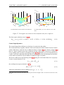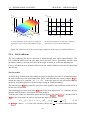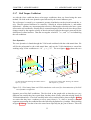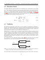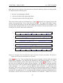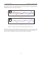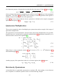
1
Autonomous Aircraft A nonlinear approach Group 1034 IAS10 - 2005 - Aalborg University by Finn Jensen Daniel René Hagen Pedersen Faculty of Engineering and Science Aalborg University Institute of Electronic Systems - Department of Control Engineering TITLE: Autonomous Aircraft: A nonlinear approach. PROJECT PERIOD: 9-10th. semester September 1st - June 2nd 2005 PROJECT GROUP: Group 1034 - 2004-2005 GROUP MEMBERS: Finn Jensen Danial René Hagen Pedersen SUPERVISOR: Jan Helbo Anders la Cour-Harbo Department of Control Engineering PRINTS : 11 Number of pages in report : 83 Number pages in appendix : 30 Total number of pages : 122 ABSTRACT: A Cessna Skylane 182 model aircraft must be stabilized and flying autonomous. An aerodynamic model is derived using Computer Fluid Dynamics and wind tunnel data from a real Cessna Skylane 182. Blade Element Theory is used to model the propeller thrust. And the dynamics and kinematics are modeled as a rigid body with 6 Degree of Freedom, using quaternions to describe the orientation of the aircraft. Nonlinear noninteractive feedback linearization is used to linearize the model. And the aircraft is stabilized using a state space controller, and the orientation is controlled by a quaternion control law. The stability of the system is verified using Lyapunov stability theorem. The models are implemented in a 3D flight simulator, and the controllers are able to control this simulator. The controllers are not implemented on the aircraft. Test flights were used to validate the models, and test the hardware platform. Further improvements can be implementing a kalman filter and make the aircraft fully autonomous and designing a path generator and controller. Preface This report serve as documentation for the 10th semester project: "Autonomous Aircraft: A nonlinear approach" in Intelligent Autonomous Systems a specialization at Aalborg University, Department of Control Engineering. References to literature are done like [7, p. 500], which refer to "Nonlinear Systems" by Hassan K. Khalil on page 500. The reference can be found in the Bibliography on page 80. A CD-Rom is attached to the report. This CD-Rom contains Matlab scripts, Simulink models and flight simulator, a controller for the simulator, results from the aerodynamic analysis, and a data logger. The CD-Rom contains also: data sheets over the hardware, software, and movies of a test flight. This report is also on the CDROM found in a pdf format. A nomenclature list is placed in the start of the report on page v, and contains variables used throughout the report. An index is found on page 112 of the report. Aalborg University, June 2nd 2005. Finn Jensen Daniel R. H. Pedersen iii Aerodynamics –the ultimate artform. When you get it right mighty beasts float up into the sky When you get it wrong people die. -Roger Bacon (c1384) iv Nomenclature α This is the angle of attack and it is defined as the angle between B x and B vB,x in the B x, B z plane. q̄ The dynamic pressure q̄ = β This is the sideslip angle of the aircraft, and it is defined as the angle between B x and B vB,x in the B x, B z plane. ρ The density of the atmosphere, ρ = 1.225 at an altitude of 100m B ω̇ B Is the angular acceleration of the aircraft and the time derivative of B ωB . Bω B 2 ρV∞ 2 . Is the angular velocity of the aircraft with respect to the inertial reference system seen from the body frame B, around the B x, B y and axes. Bz Bτ Ba is the vector torque around the B x, B y and B z axes. Linear acceleration of the aircraft in B x, B y and B z axes. B BF Is a force vector along the B x, B y and B z axes. Bv B Linear velocity vector of the aircraft in B x, B y and B z axes. V∞ Velocity of the aircraft relative to the wind. δ h The control input vector δ = δ f b The reference wing span c The reference chord line length CB τ A CB F A δa δe δr iT The dimension less aerodynamic torque coefficient. The dimension less aerodynamic force coefficient. S The reference wing area A Aerodynamic coordinate system, with origin in Center of Aerodynamics CoA, with the three axes: A x, A y, and A z. B Aircraft body fixed coordinate system with origin in the CoG and the three coresponding axes B x,B y and B z. E Earth Centered, Earth Fixed coordinate system (ECEF) with components E x,E y and E z. N Navigation coordinate system establishes a reference point for navigating the aircraft, the three axes are denoted as N x,N y and N z. R Aircraft fixed reference coordinate system with origin in the CoG and the three coresponding axes R x,R y and R z, always oriented as the Navigation coordinate system N. Pitch (θP ) Is the angle between B x and R x positive counter clockwise around the B y axis. Roll (θR ) Is the angle between B z and R z positive counter clockwise around the B x axis. Yaw (θY ) Is the angle between B x and R x positive counter clockwise around the B z axis. v Contents 1 Introduction 1 1.1 The Aircraft . . . . . . . . . . . . . . . . . . . . . . . . . . . . . . . . . . . . 2 1.2 The Aircraft Platform . . . . . . . . . . . . . . . . . . . . . . . . . . . . . . . 2 1.3 Platform Requirements . . . . . . . . . . . . . . . . . . . . . . . . . . . . . . 4 1.4 Platform Design . . . . . . . . . . . . . . . . . . . . . . . . . . . . . . . . . . 5 2 Requirements 7 2.1 Instrumentation . . . . . . . . . . . . . . . . . . . . . . . . . . . . . . . . . . 7 2.2 Modeling . . . . . . . . . . . . . . . . . . . . . . . . . . . . . . . . . . . . . 8 2.3 Control . . . . . . . . . . . . . . . . . . . . . . . . . . . . . . . . . . . . . . 8 3 Methodology 3.1 9 Report Structure . . . . . . . . . . . . . . . . . . . . . . . . . . . . . . . . . . 4 Definitions 11 12 4.1 Parts on the Aircraft . . . . . . . . . . . . . . . . . . . . . . . . . . . . . . . . 12 4.2 Coordinate Systems . . . . . . . . . . . . . . . . . . . . . . . . . . . . . . . . 13 4.3 Basic Aerodynamics . . . . . . . . . . . . . . . . . . . . . . . . . . . . . . . 15 4.4 An Aircraft with six Degree of Freedom . . . . . . . . . . . . . . . . . . . . . 19 5 Aerodynamics 21 5.1 Aerodynamic Analysis . . . . . . . . . . . . . . . . . . . . . . . . . . . . . . 22 5.2 Propeller . . . . . . . . . . . . . . . . . . . . . . . . . . . . . . . . . . . . . . 43 5.3 Aerodynamic Model . . . . . . . . . . . . . . . . . . . . . . . . . . . . . . . 48 6 Aircraft Dynamics and Kinematics 6.1 49 Dynamical Model . . . . . . . . . . . . . . . . . . . . . . . . . . . . . . . . . vi 50 6.2 Kinematic Model . . . . . . . . . . . . . . . . . . . . . . . . . . . . . . . . . 52 6.3 Validation . . . . . . . . . . . . . . . . . . . . . . . . . . . . . . . . . . . . . 52 7 Control of Aircraft 54 7.1 Feedback Linearization . . . . . . . . . . . . . . . . . . . . . . . . . . . . . . 55 7.2 Angular Velocity Controller . . . . . . . . . . . . . . . . . . . . . . . . . . . 59 7.3 Orientation Controller . . . . . . . . . . . . . . . . . . . . . . . . . . . . . . . 59 7.4 Controller Performance . . . . . . . . . . . . . . . . . . . . . . . . . . . . . . 63 8 Stability 66 8.1 Interconnected Systems Approach . . . . . . . . . . . . . . . . . . . . . . . . 66 8.2 The Stability Analysis . . . . . . . . . . . . . . . . . . . . . . . . . . . . . . . 68 8.3 The Result . . . . . . . . . . . . . . . . . . . . . . . . . . . . . . . . . . . . . 71 9 Test Flight 9.1 72 Test Flights . . . . . . . . . . . . . . . . . . . . . . . . . . . . . . . . . . . . 10 Conclusion 73 77 10.1 Perspective . . . . . . . . . . . . . . . . . . . . . . . . . . . . . . . . . . . . 78 Bibliography 79 A Data Logger 81 A.1 Gyro Logger . . . . . . . . . . . . . . . . . . . . . . . . . . . . . . . . . . . . 83 A.2 GPS Logger . . . . . . . . . . . . . . . . . . . . . . . . . . . . . . . . . . . . 83 A.3 Servo Logger . . . . . . . . . . . . . . . . . . . . . . . . . . . . . . . . . . . 85 A.4 Servo Board . . . . . . . . . . . . . . . . . . . . . . . . . . . . . . . . . . . . 86 A.5 Guide to Data Logger . . . . . . . . . . . . . . . . . . . . . . . . . . . . . . . 89 B Test Appendix 90 C Quaternions 95 D Hardware Implementation 99 Index 109 vii Chapter 1 Introduction This Project is part of an ongoing process since 2000, to design an autonomous aircraft at Aalborg University. From 2000 to 2004 the project have been based on a Graupner Trainer 60 model aircraft, and a completely linear control, and modelling approach. Unfortunately the Graupner aircraft crashed during a test flight in the last project, which damaged the aircraft and flight hardware severely. Previous Projects When reviewing the previous projects we learned that the primary task of all projects had been to develop and understanding a model for the aircraft. Unfortunately has the used model, due to the crash, never been validated or verified. Thus we could not be sure that using the previous approach would be sufficient and time effective. Combining the aircraft project history with our satellite project experience, and courses in nonlinear control, we decided to use a more theoretical and non-linear approach to the control and modelling part of the project. The Experiences The experience from the last project group was that it was necessary to acquire a large aircraft, because one of the theories to why the last aircraft crashed, was that it simply where to small to carry the flight hardware. Other experiences said that the flight hardware, where difficult to work with, mainly because of time and power issues. But there also seemed to be problems with the accuracy and noise levels of the sensory system in the previous project. Since the aircraft project had to start over again it was decided to put more effort into the flight hardware design and aircraft platform, such that the following projects have a better platform to build their projects on and calculated that it could save this project some time, if there where a 1 1.1. THE AIRCRAFT CHAPTER 1. INTRODUCTION working and easy to use platform. 1.1 The Aircraft To solve the weight problem from the last project a bigger aircraft was bought. A Cessna Skylane 182, which is 26% scale model of the real Cessna Skylane. See the front page of this report for a picture. The aircraft consist of the following basic parts: • Cessna Skylane 182 airframe • Webra BOXER 30-2 FT-Glow engine • Two Webra Speed 91-P5 silencers • Three bladed Graupner propeller • Graupner SC Receiver • Two 10.3Kgcm Hitec HS-5645MG Digital Ultra Torque servos • Two analog Futaba servos • Four 4.4Kgcm Hitex HS-5475HB Standard Digital servos. • 0.5l fuel tank The total weight without Flight hardware is: 7.5kg. The aircraft is manually controlled using a Graupner mx-22 remote control. 1.2 The Aircraft Platform The previous group[2] designed the system shown in figure 1.1. The individual parts on figure 1.1 are described below PC-104 The system was build on the Simulink toolbox xPC-target. A small real time operation system where installed on the PC-104. It was then possible to download programs into the PC-104, and execute them from a desktop PC. The interface between the PC-104 and the desktop PC was a RS-232 connection. GPS & GSM Modem A GPS of the type Lassen SK II was used to determine the position, and velocity of the aircraft. It was chosen to used dGPS, so the position can be determined more precise, and a GSM modem of the type Siemens M20 was used. 2 CHAPTER 1. INTRODUCTION xPC Interface dGPS 1.2. THE AIRCRAFT PLATFORM RS232 RS232 PC-104 GSM Modem with Orientation Sensing module RS232 Reciever xPC-target Switch Servo interface Gyroscope (Pitch) Filter 4× Servo motors Gyroscope (Roll) Figure 1.1: Overview of the system on the Grupner aircraft Orientation Sensing module was of the type TCM2 Electronic Compas module. This module measured the pitch and roll angle of the aircraft. The module could also measure the electro magnetic field of the earth in three axis and the temperature of the air. Interface to the PC-104 was a RS232 serial connection. Gyroscope was used to measure the change of the angle in one direction. Two gyroscopes were used in the aircraft. One measured the angular velocity in pitch direction, and the other gyroscope measured angular velocity in roll direction. The output from the gyroscope was a voltage between −2.5V and 2.5V Filter The signal from the gyroscopes was filtered to remove noise on the signal. Switch The aircraft had to be able to fly in 2 modes. One mode was autonomous mode where control algorithms control the aircraft. The other mode was manuel mode where a pilot on the ground controlled the aircraft. The switch was used to shift between the two modes. Receiver The receiver get the control signals from the pilot on the ground. This receiver used Pulse Code Modulation (PCM). It was a Robbe Futaba PCM 1024. Servo Motors The actuators, which were used to control the aircraft, were four servo motors. The input to the motors were a PWM signal, which controlled the servomotors. Servo interface had different tasks in autonomous and manuel mode. In autonomous mode it controlled the servomotors with PWM signals updated with an interval on 20ms. The control signal came from the PC-104. In manuel mode it measured the position of the servos, and sent it to the PC-104. The interface between the PC-104 and the servomotors was implemented in a PIC 16F877. The experience from the last project [2] showed that XPC eased the implementation. There is two problem which need to be solved, the data storage, and download time, thus it is needed to 3 1.3. PLATFORM REQUIREMENTS CHAPTER 1. INTRODUCTION find a solution such that the data wasn’t lost if the system powered off and such that the download time is shorter. Another reusable design is the switching mechanism between autonomous and manual mode worked. Another experience from both the last aircraft project and the autonomous helicopter project same year, told that heating and noise was a great issue, thus some effort needed to be placed in the EMC design of the platform, and cooling the platform. 1.3 Platform Requirements To make this platform usable in future project a feasibility study was conducted, to find the requirements for the hardware platform and the following was the conclusion of this feasibility study. The conclusion is divided into control tasks for which a sensor type is specified. Stabilization requires information from the angular rates of the aircraft. The best solution is Gyro measurements of all 3 axes of the aircraft. Orientation requires measurements to some external reference, here the magnetic field of the earth or the gravitational field could be used. Flight path The best solution for this is GPS or similar systems, but the accuracy restricts this sensor to pure flight, thus another system is needed during autonomous landing and takeoff. The feasibility study also contained safety issues and handling issues. This resulted in the following requirements. Manual override is a requirement to ensure that the aircraft isn’t lost if anything should go wrong. Thus it is necessary to ensure that the platform never could take the control of the aircraft without acknowledgement from ground. It should always be possible to manual override any commands from the flight platform. The power usage of the platform is required to be low, such that the runtime of the hardware platform is extended. Safe mode It is necessary that the aircraft is manually controllable even if the flight computer is powered off. It is a requirement that the flight computer and servo motors have different power supplies, such that the manual flight time isn’t reduced due to errors or short circuits in the flight computer. Data storage must be non-volatile such that sensor data and logs aren’t lost if the flight computer should shutdown. Download time must be minimized such that it is possible to download data between test flights without waiting to long and using flight power. 4 CHAPTER 1. INTRODUCTION 1.4. PLATFORM DESIGN Data logging must be carried out in a simple and effective way, such that the measurements of each test case are easy to acquire. The raw data from the measurements should be saved, such that no details are lost in the processing of the data. 1.4 Platform Design The new platform, which have been designed such that the requirements in section 1.3 are satisfied is described in this section. A user guide for the XPC system can be seen in appendix A.5. The design is based on two individual parts the critical hardware and Flight Computer (FC) see figure 1.2. The critical hardware covers the Servo Controller and Interface Card (SCIC). 1.4.1 Servo Controller and Interface Card The SCIC is designed such that it uses a minimum of power and such that it works even if the servo battery voltage drops lower than the input range of the receiver and servos. • The SCIC is also design such that it are able to measure the servo input signals and this way read the position of the servos. • Another feature shown on figure 1.2 is the switching mechanism which allows the MCU and Flight computer to control the output signal to the servos. This mechanism is designed such that the ground controller at any time can override the MCU. • The SCIC is also independent of the FC. Thus no matter which state the FC is in the SCIC always works, as long as there are power on the Servo battery. • The MCU software is design such that it cannot do any damage to the aircraft, by limiting the servo output ranges. 1.4.2 Flight Computer As shown on figure 1.2 the FC contains a Power Supply unit (PSU), mass storage device (MASS), GPS, GyroCube, and inteface to: VGA, RS232, reset, keyboard, and mouse. • The PSU is a switch mode power supply, with a 95% efficiency. It requires an input voltage between 8 − 15V and delivers: 3.3V, and 5.0V output to the entire FC. • MASS is a 256MB IDE Flash disk, only used for saving measurement data. • The GyroCube is a combination of a three axes Gyro and a three axes accelerometer. Thus providing the platform with sensors to the stabilize and orientation requirements in section 1.3. 5 1.4. PLATFORM DESIGN CHAPTER 1. INTRODUCTION Flight Computer 12V Battery 1 Battery 2 PSU PC104 IDE GPS Interface RS232 VGA RS232 Reset Key/Mouse ADC PSU Receiver Inputs Reciever Input GyroCube D I/O Servo Controller and Interface Card Battery MASS Samplings board MCU Switch Servo Output PWM Power Figure 1.2: Overview of new hardware platform, including: PC104, Power supply units (PSU), sensors, and Servo Controller and Interface Card (SCIC). • The GPS is a SBAS1 enhanced GPS receiver from Novatel with an accuracy down to 2m[12]. 1 SBAS is ESA’s Satellite Based Augmentation System, which provides satellite based differential GPS signal thru EGNOS [4]. 6 Chapter 2 Requirements This chapter contain the requirements for the project. The requirements are divided in three parts: hardware, software, and instrumentation, a part about modeling the aircraft, and a part about controlling the aircraft. The main goal for the project is: The Cessna Skyline 182 model aircraft must be able to fly autonomously. To reach this goal the following requirement have to be meet. Not all the requirements is equal important, so a prioritizing is made from A to C, where A is the most important. 2.1 Instrumentation All hardware and software requirements are high priority, because it is necessary for the autonomous flight. SPEC-1,1 Instrument the Cessna Skylane 182 aircraft model with: sensors, actuators, interfaces, batteries, and flight computer.(A) SPEC-1,2 Implement a data logger including drivers to all sensors and actuators, which are able to log the following: • Positions (A) • Angular rates (A) • Accelerations (A) • Servo positions (A) SPEC-1,3 Verify that hardware and data logger work in a test flight.(A) 7 2.2. MODELING CHAPTER 2. REQUIREMENTS SPEC-1,4 In order to prevent the aircraft from crashing these two requirements must be satisfied. • Implement manual override.(A) • Implement safe mode.(A) 2.2 Modeling SPEC-2,1 Derive a model of the aircraft such that it enables autonomous flight. This includes: • An dynamic model.(A) • A kinematic model.(A) SPEC-2,2 Validate the model by flying with the aircraft model in a flight simulator.(A) SPEC-2,3 Validate the models with data from test flights.(B) SPEC-2,4 Design a Kalman filter to filter data from the sensor measurements. • Use it to filter data from the test flight. (B) • Implement a Kalman filter which run under a test flight and is used to filter the measurements for the controller.(C) 2.3 Control SPEC-3,1 Design a nonlinear controller to stabilize the aircraft by controlling the angular velocity. • Implement the controller on the flight simulator.(A) • Implement the controller on the aircraft.(B) SPEC-3,2 Design a controller to control the orientation of the aircraft. • Implement the controller on the flight simulator.(A) • Implement the controller on the aircraft.(C) 8 Chapter 3 Methodology This chapter contains a description of the overall approach of modeling and controlling the aircraft. The different methods used in modeling and control are described in this chapter. This chapter is also used to tell how the rest of the report is structured. The last section of this chapter contains a short description of the chapter contents throughout the report. The objective of this project is to make a model aircraft fly autonomously. In order to do this it is necessary to make a model of the aircraft, and design a controller, which can control this model. This has been done with the design in figure 3.1. This design split the model part up in four parts, an aerodynamic model, a propeller model, a dynamic model, and a kinematic model. It is chosen not to model the servomotors, because the they have a position controller, which can keep the position. They react also so fast compared with the rest of the system, that the dynamic from the servos would have no influence on. The controller is split in: a feedback linearization, an angular velocity controller, and an orientation controller. The methods chosen to solve each part is described in the following: Chapter 5 Aerodynamic model Chapter 7 Angular velocity controller Feedback linearization Chapter 6 Dynamic model Kinematic model Propeller model Orientation controller ref Figure 3.1: The figure shows the main parts of the system, which include an aerodynamic model, a propeller model, a dynamic model, a kinematic model, feedback linearization, an angular velocity controller, and an orientation controller. 9 CHAPTER 3. METHODOLOGY Aerodynamic model is used to calculate the size of the forces generated on the aircraft, when it is flying through the air. Dimensionless coefficients are used to calculate these forces. This method is chosen because the coefficients is independent of the size of the aircraft, only the shape matters. It is therefore possible to take the coefficients from a real Cessna Skyline 182, and used these coefficients on the model aircraft. Two methods are used to calculate these coefficients. Data from a wind tunnel test for a real Cessna 182 is combined with the Computer Fluid Dynamics (CFD) to calculate the coefficients. The wind tunnel data give the accurate values, while CFD give a better model understanding. The output from this model is coefficients used to calculate the forces and torques acting on the aircraft. The calculation of the coefficients demands a lot of CPU power, and it is impossible to make the calculation in real time on the PC-104. The result is therefore fitted with polynomials, which is execute must faster. Propeller model calculate the thrust generated by the propeller when the aircraft is flying through the air. It is not possible to control the propeller autonomously, only the pilot would have control over the propeller. The propeller is therefor handled as a disturbance. The model is used to find the size of the thrust generated by propeller as a function of the angular velocity of the propeller and the velocity of the aircraft. The model for the propeller is found by analyzing the generation of thrust in the working area for the propeller. A polynomial is then fitted to the result of the analysis. Dynamic model calculate velocity and angular velocity of the aircraft, when forces and torques is applied to the system. This model treat the aircraft as a rigid body with 6 degree of freedom. The input for this model is the output from the calculations in the aerodynamic model, and the propeller model. kinematic model calculate the orientation of the aircraft. The purpose of the project is to make the aircraft fly autonomously where the orientation of the aircraft is controlled, but is should not be able to track a path. It is therefore not necessary to have a kinematic model describing the position of the aircraft. The orientation of the aircraft is described using quaternions. This method is chosen because the solution contains no singularities. A rotation contains only matrix multiplications, which is well suited for a computer. Feedback linearization linearize the three models with respect to the angular velocity. This method is a nonlinear control technique, which require a precise model, because nonlinearities is canceled out. Angular velocity controller is a state space control, which stabilize the angular velocity. Orientation controller is a second control loop, which control the orientation represented by a quaternion. The main tools used in this project are Matlab and Simulink. 10 CHAPTER 3. METHODOLOGY 3.1. REPORT STRUCTURE 3.1 Report Structure This section contains a description of the structure for the remainder of the report. Chapter 4, 5, and 6 are modeling of the aircraft. Chapter 7, and 8 are control of the aircraft, while 9 is the result of the test flights. Chapter 4 contains the definitions used in the entire report. This include defining the important parts of the aircraft, definition of the different coordinate systems, defining basic aerodynamic terms, and explain the notation used in this report. Chapter 5 contains the aerodynamic analysis of the aircraft. This include finding the aerodynamic coefficients, and derive the aerodynamic model. This chapter include also the propeller model, because it is very similar methods, which is used to find the two models. Chapter 6 describes the rigid body dynamics and kinematics model of the aircraft. Chapter 7 contains the controller design, including a nonlinear noninteracting feedback linearization, an angular velocity controller, and a orientation controller. Chapter 8 contains a stability analysis of the aircraft model, to check the model for stability. Chapter 9 contains the results of the test flights, which has been performed with the aircraft. 11 Chapter 4 Definitions This chapter contains definitions used through out the project. Starting with naming the basic parts of the aircraft. Then defining relevant coordinate systems used to structure and simplify the modeling and control of the aircraft. Followed by a description of parameters and nomenclatures used in the project. 4.1 Parts on the Aircraft This section defines the parts of the aircraft, which is relevant for modeling and control, see figure 4.1. Rudder δr Propeller Wing Right aileron δa Vertical stabilizer Wing yaw Flaps δ f Fuselage Pitch Flaps δ f Right aileron δa Roll Horizontal stabilizer Elevator δe Figure 4.1: The different parts of the aircraft is defined. Wing The function of the wing is to generate the main part of the lift necessary to make the air craft fly. There is two control surfaces on the wing: aileron, and flaps. 12 CHAPTER 4. DEFINITIONS 4.2. COORDINATE SYSTEMS Aileron is used to change the roll1 rate of the aircraft. Since the two ailerons work opposite of each other. The control input to the aileron is the deflection angle δa , which is the angle between the two aileron, such that the angle is positive counter clockwise the B y-axis. Flaps are used as air brakes, to reduce the absolute speed of the aircraft during landing. The control input is defined as δ f Horizontal stabilizer is used to stabilize the pitch angle. Elevator is the control surface used to control the pitch rate. The control input is the deflection angle δe , which is the angle between the elevator in start position and the current angle. Positive counter clockwise the B y axis. Vertical stabilizer is used to stabilize the yaw rate. Rudder is the control surface used to control the yaw rate. The control input for the rudder is the deflection angle δr , which is the angle between the rudder in start position and the current position, positive counter clockwise the B z axis. Fuselage is the body of the aircraft. it contain the flight computer, sensors, and batteries for servomotor and flight computer. Propeller is the thrust generating part of the aircraft. 4.2 Coordinate Systems In order to model and control the aircraft it is necessary to define several coordinate systems [13, p. 320]. The different coordinate systems are shown on figure 4.2 and 4.3, and is defined in the following. Earth-Fixed coordinate system (E) rotates with respect to the earth and is centered in the middle of the earth. It rotates around E z, which points toward the north pole. E x goes through the intersection of the Greenwich meridian and equatorial plane, E y is perpendicular to both E x and E z see figure 4.2. This coordinate system is referred to as the Earth-Centered, Earth-Fixed coordinate system abbreviated ECEF. The GPS receiver gives the position in this coordinate system. We use the this coordinate system as in inertial system2 , which is valid, since the aircraft fly in a small area in short time. Aircraft body fixed coordinate system (B) is fixed to the aircraft with origin in Center Of Gravity (CoG). Figure 4.3 shows the placement of B in the aircraft. B x lies on the aircraft centerline through the tip and CoG, positive in the direction of forward motion. B y is perpendicular to B x, aligned with the wing and positive in the direction of the right wing tip. B z points downwards and is perpendicular to the two other axes B x and B y see figure 4.3. 1 2 Roll, pitch, and yaw is a rotation around B x, B y, and B z. An Inertial system is coordinate system which is at rest thus haveing either zero or a constant velocity. 13 4.2. COORDINATE SYSTEMS CHAPTER 4. DEFINITIONS North Pole E z Bx Rx CoG Bz R y,B y Nx Rz Nz Greenwich meridan Center Ny E E y 90◦ East x Equator Figure 4.2: Shows Earth-fixed E, Aircraft bodyB and Aircraft Reference R coordinate systems are related to each other. Rx Bx V∞ Az Ay Ay By B x V∞ CoA CoG Rx CoG Ax Ax Ax Ry Rz B z Center line Figure 4.3: The figure show the placement of the body fixed coordinate system B and the Aircraft fixed reference coordinate system R in the orientation for level flight. 14 Cen ter l ine CHAPTER 4. DEFINITIONS 4.3. BASIC AERODYNAMICS Aircraft fixed reference coordinate system (R) is used to establish a reference for the controller. It is centered in CoG of the Aircraft and the orientation is given by the field where the aircraft takeoff and land. R z points toward the center of the earth. R x is parallel with the runway. R y is perpendicular to the two other axes. Aerodynamic coordinate system (A) is used in the analysis of: the aerodynamic forces. A has origin in the Center of Aerodynamics (CoA) approximately C4 from the leading edge3 of the wing. A x is parallel with B vB , and positive in the direction of V ∞ . A y and A z is aligned with B y and B z when α and β are zero. Navigational coordinate system (N) is used to describe the position of the aircraft with respect to starting point of the flight. N is aligned with R, and fixed in the point where the origin of R is placed in the start of a flight. 4.2.1 Rotation between coordinate systems Several methods exits to describe the orientation of B with respect to E and to rotate a vector from B to E. In this project rotations are done using quaternions. Appendix C on page 95 describes quaternions and how the are used to rotate a vector from one frame to another. Some properties of Quaternions are that: there are no singularities in the solution, only four parameters is used instead of nine as for Euler angles, and it is less computer demanding. The nomenclature for a quaternion is in this project as follows: BE q is the quaternion, which represent the rotation from E to B. "E # ωB B ∗ B B ωB = E q ⊗ ⊗ Eq (4.1) 0 Where: E ωB is interpreted as the angular velocity of B, measured in E with respect to E our inertial system. BE q∗ is the complex conjugated quaternion of BE q, ⊗ represent quaternion multiplication, and B ωB is the angular velocity of B, still measured with respect to E but seen from or rotated to B. (4.2) rotates back again. E # ωB B ⊗ Eq ωB = q ⊗ 0 B E ∗ "B (4.2) 4.3 Basic Aerodynamics This section defines the basic aerodynamic forces: lift, drag, and side-force, which is generated when the aircraft is flying through the air. A model is derived in chapter 5, covering the aerodynamic forces and torques. In order make this model the geometry of the airfoils are defined. 3 Chord line and leading edge is defined on figure 4.6 15 4.3. BASIC AERODYNAMICS CHAPTER 4. DEFINITIONS 4.3.1 Aerodynamic Forces In general an aircraft is flying because a force called lift is greater than the gravitational force. As seen on figure 4.4 four forces is acting on an aircraft: Lift, Drag, Thrust and Gravity. Gravity is strait forward to determine. The difficult part is: thrust, lift, and drag forces. These forces are determined by the aerodynamics that describes the forces generated by an object moving through gases(atmosphere). Lift When a object is moving through a gas a resulting force is created on the object. This force depends of: the geometry of the object moving through the gas, velocity of the object, angle of attack, and slipping. The component of the force which is perpendicular to the direction of motion between the gas and the aircraft is called Lift. If the lifting force gets greater than the gravity force then the aircraft is flying. Lift Drag Thrust Gravity Figure 4.4: Shows the four forces Lift, Drag, Thrust and gravity on the aircraft Drag In general drag is the force, generated by a solid object moving through a fluid or gas, oppose the direction of movement. There are different sources for drag: one is Skin Friction which is generated due to the friction between molecules and the solid object[3]. Another source is the form drag which is generated due to pressure changes around an object and adding all the forces up, the form drag force is the force projected onto the vector oppose the direction of movement through the air[3], also defined as the A x-axis. Thrust Thrust is caused by the propeller, which in fact are rotating wings. This rotation courses a lifting force to be created in the direction of B x. This lifting force is defined as the Thrust. 16 CHAPTER 4. DEFINITIONS 4.3. BASIC AERODYNAMICS Torque The two forces lift and drag are generated all over the aircraft and vary with the control surfaces: Flaps, Aileron, Elevator, and Rudder. These force are applied at different distances to the CoG thus causing a torque on the aircraft and making it rotate around B x,B y and B z. 4.3.2 Airfoil The airfoil geometry is an important factor, when lift and drag are calculated. The geometry used to describe an airfoil is defined in this section. A 3 dimensional wing is shown on figure 4.5, while figure 4.6 shows the wing in B xB z-plane. The front of the wing is called the Wing z−coordinate 3−D Airfoil 0.1 0 −0.1 Span Chord Symmetry line 1 Trailing Edge 0.5 CoA 0 Wing y−coordinate −0.5 Leading Edge −1 0.2 0 Wing x−coordinate Figure 4.5: The figure show: leading edge, trailing edge, CoA, Chord, and span, on the wings. leading edge, the back of the wing is called the trailing edge. The length between the leading and the trailing edge is the chord length. Because the wing is not a rectangle the chord vary along the span. An important property of the wing is the Center of Aerodynamic pressure 17 4.3. BASIC AERODYNAMICS CHAPTER 4. DEFINITIONS (CoA). CoA is for aircraft with low velocity placed on a axes which lie a 14 chord from the leading edge [3]. CoA is placed on the symmetry line. The aerodynamic forces lift and drag is generated in this point, while the torque work around the axes of B. Upper Surface Leading Edge Trailing Edge Lower Surface CoA Chord line Mean Camber line Figure 4.6: An airfoil is shown with: surfaces, chord line, leading edges, Trailing edge, and CoA. 4.3.3 Important Aerodynamic Parameters Important parameters for the generation of lift and drag is: geometry of the wing, angle of attack, and slipping. Slipping and angle of attack is defined in this section. −B z Chord line α v∞ B x CoG Figure 4.7: Definition of angle of attack α, and V∞ . V infinity is the relative wind speed(V∞ ). It is the speed of the air toward the aircraft. It is assumed that there is no wind, thus V∞ = |−B v|. Angle of attack Angle of attack (α) is an important parameter for the stability of the aircraft in the vertical plane. The lift of the plane is dependent of this parameter, and a change in α gives changes in lift and drag. α is defined as the angle between B v the chord line in the wings, see section 4.3.2, and velocity vector V, thus α = arctan B vxz . Side slipping in the horizontal plane, the slipping angle (β) an important stability parameter and can be seen on figure 4.8. It describes the angle between B x and the velocity vector B vB , in the B xB y-plane. β is given as: β = arcsin 18 Bv B,y V∞ CHAPTER 4. DEFINITIONS 4.4. AN AIRCRAFT WITH SIX DEGREE OF FREEDOM B x β V B y Figure 4.8: Definition of slipping angle β. 4.4 An Aircraft with six Degree of Freedom The aircraft can perform six different motions. Three of these are translatorial motions along the axes of B with respect to E and three are angular rotation of B with respect to E. This gives a system with 6 Degrees of Freedom (DoF), which is shown on figure 4.9. The figure also shows the notation used for the vector components of: force, torques, velocity, and acceleration. Forces, velocities and accelerations are all given in vectors, which have three components as it is shown in figure 4.9. As an example the angular velocity vector B ωB shown in (4.3). This vector is seen from B and measured with respect to E. B ωB,x B ωB = B ωB,y (4.3) B ωB,z A description is given of all the vectors used to describe motions and forces in table 4.1. 19 4.4. AN AIRCRAFT WITH SIX DEGREE OF FREEDOM CHAPTER 4. DEFINITIONS Lateral axis B y B B B E vB,y , E aB,y , F y B B B E ωB,y , E ω̇B,y , τy Longitudinal axis B B B E vB,x , E aB,x , F x CoG B x B B B E ωB,x , E ω̇B,x , τ x B B B E ωB,z , E ω̇B,z , τz B B B E vB,z , E aB,z , F z B z Vertical axis Figure 4.9: Definition of: velocity, acceleration, forces, angular velocity, torques, and angular accelerations on the aircraft. Unit v a F ωB ω̇B τ Description Velocity of the aircraft Accelerations Linear forces Angular velocity of B Angular acceleration of B Torque Type Translatorial Translatorial Translatorial Angular Angular Table 4.1: Forces, velocities, and accelerations on the aircraft. 20 Chapter 5 Aerodynamics This chapter contains an analysis of forces and torques generated by the air flow around the Cessna 182 Skylane aircraft. The flow arround the aircraft is analysed through Computer Fluid Dynamics (CFD) simulations. The CFD simulation results are combined with Wind tunnel data [14] to model the aircraft more accurately. The resulting forces and torques are then determined from the general aerodynamic force and torque equations. To simplify the modelling process we choose to divide the aircraft aerodynamics into two parts: The aerodynmics, and the Propeller dynamics, as on figure 5.1. V∞ ,α,β B ωB ,δ,ρ Cessna 182 Aerodynamics B B FA τA B + V∞ ,α,β ωP ,ρ Propeller Thrust dynamics B B B Faero τaero FP τP Figure 5.1: The different aerodynamic models covered in this chapter: Cessna 182 model, and Propeller thrust model. In addition figure 5.1 shows the inputs to the models: Density of the atmosphere ρ, Relative h iT wind speed V∞ , angle of attack α, sideslip angle β, control inputs δ = δ f δa δe δr , ωP the angular velocity of the propel, and B ωB the angular rates of the aircraft. These inputs are feed to the aerodynamic models, which returns the respective aerodynamic forces: B FA , and B FP , and torques: B τA , and B τP . The sum of the forces is denoted as B Faero and the torques B τaero . The main problem in modeling aerodynamics is to find an expression for the aerodynamic forces and torques. For this purpose we use the standard equation for aerodynamic force (5.1) 21 5.1. AERODYNAMIC ANALYSIS CHAPTER 5. AERODYNAMICS and aerodynamic torque (5.2) [3], B FA = q̄S CB FA b 0 0 B τA = q̄S 0 c 0 CB τA 0 0 b (5.1) (5.2) where q̄ is the dynamic pressure and S ,b,and c are the reference: Surface area, span, and chord length . CB FA and CB τA is the dimension less aerodynamic force and torque coefficients. The dimension less property of the coefficients, is used such that the coefficients don’t depends on the size and length of the aircraft only the shape. Instead special reference lengths b and c are used to scale the size of the aircraft. The aerodynamic coefficients characterise the aerodynamic properties of the aircraft. Thus it is essential to find these coefficients to model the aerodynamics. All aerodynamic literature in this project is based on designing an aircraft, which full fill a curtain aerodynamic characteristic. This Project is the reversed problem, the aerodynamics properties of a given aircraft must be found. Thus the methods used in this project are based on a reverse engineered design of an aircraft. To find the coefficients, there are different design approaches: wind tunnel testing, test flights or CFD simulations. This project uses a combination of all three methods. The reason for using a combination is to reduce the final model error, thus making better conditions for the nonlinear feedback linearization later on in chapter 7.1, because the linearization method requires a precise model of the aircraft, to be able to cancel the right nonlinearities. Since the simulations are very computational demanding we will use polynomial fits to calculate the coefficients at runtime. This approach reduces the computational demand of the model. 5.1 Aerodynamic Analysis This section contains an aerodynamic analysis of the Cessna 182 Skylane. The analysis of the propeller will follow in section 5.2. To model the aerodynamic forces on an aircraft, it is nescessary to find the aerodynamic characteristics. This could be done in various ways, where a simple and efficient method is the Vortex Lattice Method (VLM) [8], which is described briefly in the following section. Another more accurate method is to perform experimental wind tunnel tests. In this project we derive our aerodynamic model from both methods, and we use test flights to validate the model. 5.1.1 Vortex Lattice Method VLM is a method for modelling flow around objects. This is done by panelizing the surface of the airfoils see figure 5.2 and calculating the airflow on each panel. This method is unfortunately very computational demanding, thus not suitable for online calculations. VLM uses 22 z−axis CHAPTER 5. AERODYNAMICS 0.2 0.1 0 5.1. AERODYNAMIC ANALYSIS δr δa δf 1 δe 0.5 CoA Symmetry line 0 −0.5 y−axis −1 0.5 x−axis 0 1 Figure 5.2: The panelized airfoil configuration of the Cessna 182 Skylane, with δ f = 15◦ flaps, aileron deflection δa = 10◦ , elevator deflection δe = 10◦ , and rudder deflection δr = −10◦ . The airfoils is visualised in the A coordinate system, with origin at the intersection of leading edge and the symmetry line of the wing. The CoA is shown in the point where the Mean Aerodynamic Chordline (MAC) and Symmetry line intersects marked by a ball. the Cartesian coordinate system referred to as the aerodynamic coordinate system A, which is shown on figure 5.2 with α = 0, and β = 0 and described in section 4.2. VLM is restricted to describing inviscid and incompressible flow, meaning low speed subsonic flow1 , where skin friction is disregarded. These flows are efficient modelled through an idealised flow theory called Potential Flow Theory[8], which is used in the VLM together with thin airfoil theory[8], which disregards thickness effects2 . In Potential Flow Theory any flow is modelled as a superposition of the elementary flow types: Uniform flow, Sinks and Sources, Doublets, and Vortices see the description below: Uniform flow is a constant flow, like the flow of water from a water tap. Sinks and sources is describing the flow, where water is flowing to or from a single point. The drain from a sink is a Sink flow and the flow into a sink is a Source. Doublets are a special combination of sinks and sources placed in the same point. Vortices is describing the rotating flows, like when water runs down the drain of sink it makes a spiral turning flow. A low speed subsonic flow is a flow with a Mach number M = Va < 0.2, a is the speed of sound 340.3m/s and V is the flow speed. This is a rule of thumb stating: that most airfoil shapes never experience local supersonic flow at Mach numbers < 0.2. 2 Thickness effects are the effects caused by the shape of the airfoil, where thin airfoil theory only investigates the aerodynamics of the mean chord line curve. 1 23 5.1. AERODYNAMIC ANALYSIS CHAPTER 5. AERODYNAMICS To describe the flow over an airfoil a combination of all the elementary flow are needed, but experiments have shown that to describe the lifting forces a combination of vortices and uniform flow is sufficient to a high degree of accuracy [8]. VLM is designed to model lifting forces, thus it uses the combination of vortices and the uniform flow to describe the flow around an airfoil. The induced flow3 from all panels including itself are calculated and summed up, to determine the flow on each panel. A Matlab implementation of this rather complex algorithm is named Tornado, and is used in this project to simulate the aircraft aerodynamics and determine the aerodynamic coefficients of interest. Since the VLM method don’t estimate drag except induced drag, which is directly dependent on lift, we use the wind tunnel data to model the effects of drag and fuselage. Instead when the VLM result is free of dampening from drag, it gives better insight into and understading of the dependencies of the aerodynamic coefficients. The VLM method is also disregarding the fuselage, which have a great influence on specific parts of the aerodynamic coefficients. Due to the lee of the fuselage. For instance the influence on the vertical stabilizer is damped from changes in angle of attack, because the fuselage force the air to move in a different path around the fuselage. We have used the VLM simulations in this project to get a more detailed and practical insight into aerodynamics. 5.1.2 Wind Tunnel Testing The most accurate way to determine the aerodynamics coefficients of an object, is experimental wind tunnel testing. Since the aerodynamic coefficients are normalised to the wing area S , wing span b and mean chordc, it is possible to reuse wind tunnel data from a real size Cessna Skylane 182. The only demands are that the right reference length for the model aircraft are used in (5.1) and (5.2). Since wind tunnel data includes all aerodynamics effects it is more acurate to use. Thus this project uses the wind tunnel data to fit the coefficients to. Since there to some coefficients only consists of two samples, is the VLM result used to verify, that it agree with the wind tunnel data[14], and that there is a linear relation in these cases. 5.1.3 Aerodynamic Coefficients There are six aerodynamic coefficients describing the aerodynamics of an aircraft, all depending on various inputs: relative wind speed V∞ , angle of attack α, side slip angle β, angular rates B ωB and control deflection angles: δ. See table 5.1. The coefficients in table 5.1 are found through a combination of the VLM, and wind tunnel data. To reduce the online calculation it is chosen to use simple polynomial fits to represent the coefficients. It is noted from table 5.1 that the force coeffients are given in the aerodynamics frame A and 3 An Induced flow is a flow caused by another flow, just like an induced current from an electromagnetic field. 24 CHAPTER 5. AERODYNAMICS Coefficient name Drag Side force Lift Rolling torque Pitching torque Yawing torque 5.1. AERODYNAMIC ANALYSIS Nomenclature CA F x (α, β, B ωB , δ, V∞ ) CA Fy (α, β, B ωB , δ, V∞ ) CA Fz (α, β, B ωB , δ, V∞ ) CB τx (α, β, B ωB , δ, V∞ ) CB τy (α, β, B ωB , δ, V∞ ) CB τz (α, β, B ωB , δ, V∞ ) Table 5.1: The standard aerodynamic coefficients and there dependencies the torques are given in the body frame B. This is the standard representation of aerodynamic coefficients since it ease the experiment process, and because the definition of the aerodynamic force tells that they are aligned with the wind direction. The aerodynamic torque is in relation to the body axes of an aircraft. Before analysing the VLM simulation result and wind tunnel data, we look at the aerodynamic coefficients, and set up a goal for the analysis. We want to find the six coefficients for the Cessna skylan 182 model aircraft and to ease the task on linearizing the model later on we want to find the coefficient on the following form. CA F (α, β, B ωB , δ, V∞ ) = CA Fzero (α, β, B ωB , V∞ ) + CA Finput (α, β, δ)δ CB τ (α, β, B ωB , δ, V∞ ) = CB τzero (α, β, B ωB , V∞ ) + CB τinput (α, β, δ)δ (5.3) (5.4) where CA Fzero (α, β, B ωB , V∞ ) and CB τzero (α, β, B ωB , V∞ ) are the zero dynamic terms with respect to the control inputs, and CA Finput (α, β, δ) and CB τinput (α, β, δ) are control input influence coefficient. 5.1.4 Drag Coefficient The drag coefficient is a coefficient with a big complexity, due to the various parameters causing drag: skin friction, fuselage, boundary layer effects4 , turbulence and lift. Since the VLM simulation only takes the lifting influence (induced drag) into account it is a very pour method to represent drag in general. Instead we will fit the drag coefficient to the wind tunnel data, which includes all the effects above. Zero Dynamics To find the zero dynamic part of the drag coefficient, we will look at the part of the drag data, which is independent on the control inputs. Thus looking at dependencies regarding to angle of attack and sideslip. The reason for not looking at the angular velocities B ωB is that the resulting influence on drag is neglegible. We will use the wind tunnel data to fit the drag coefficient, and use VLM result to show that the valid range of the wind tunnel data is larger than given in the wind tunnel data Figure 5.3 shows both differences and equalities between the wind tunnel data 4 Boundary layer effects are the aerodynamic effects caused by the difference in air velocity, in different distances from the surface of the aircraft. The air particles just on top of the surface are not moving at all. 25 5.1. AERODYNAMIC ANALYSIS CHAPTER 5. AERODYNAMICS CAF 0.2 x,zero CAF x,zero 0.1 0.15 0.05 0.1 0 0.05 −0.05 −5 Wind tunnel data The fit 0 0 β 5 −10 0 α 10 −0.05 −5 (a) VLM simulation of the Drag coefficient. 0 5 α 10 15 20 (b) Wind tunnel data from a real Cessna 182 Skylane [14]. Figure 5.3: Data used to determine the zero-dynamics Drag coefficient CA F x,zero (α, β). and the VLM. At high angles we see that figure 5.3(b) includes turbulence or stall effect on the drag coefficient, which isn’t included in the VLM result on figure 5.3(a). It is seen that at low α, the induced drag term dominates the drag coefficient, thus the range of the coefficient is extendable in the negative angle of attack direction α ≥ −10◦ . CAF 0.02 x,zero 0.01 0 −0.01 −0.02 −5 0 β 5 Figure 5.4: Wind tunnel data the β drag relation. The side slip relation on figure 5.4 is also seen on the contur curves of figure 5.3(a), thus this dependecy is taken into account in the aircraft model. To fit the coefficients we use a least square fit of the wind tunnel data. By using the wind tunnel data instead of the VLM we have achieved to extend the detail of the model by including stall at high angle of attacks α ≥ 15◦ . 26 CHAPTER 5. AERODYNAMICS 5.1. AERODYNAMIC ANALYSIS The least square fit for the zero dynamics is found using the following polynomial candidate (5.5). h iT (5.5) CA F x,zero (α, β) = CA F x,0 + PTA F x,zero (α) α β The candidate function is found through an iteration of different candidates for the VLM data, until the best candidate, resulting in the lowest fit error variance, where found see (5.6). The reason for not having the α3 term is that CA F x,zero wound have a to flat slope. The zero dynamics parameter vector are fitted to (5.6), and the constant CA F x,0 = 0.027 represents the skin friction. h i PTA F x,zero (α) = 0.22211 + 2.5785α − 53.4504α4 0.17 (5.6) Control Input Dynamics We look at the control inputs influence on the drag coefficient, in the same way as for the zero dynamics. One issue here is to identify which control surfaces influences the drag coefficient. It turns out to be the flaps of the aircraft since it is the only one with a non-negligible effect. Even though this is out of the scope of this project we include this into the model to ease future projects. CAF 0.1 x,input 0.05 0 0 α 10 20 30 20 δf 10 0 Figure 5.5: Wind tunnel data of flap influence on drag from a real Cessna 182 Skylane [14]. The retalion between flap control input δ f , and α to the drag coefficient is shown on figure 5.5. We don’t use the VLM data at this point since it don’t handle drag simulation as turbulence which is the main cause for the drag change on the aircraft due to flap deflection. The least square candidate used to fit the control influence is (5.7). CA F x,input (α, δ) = PTA F x,input (α)δ f (5.7) The control input influence coefficient is then fitted to (5.7), where δ f is the flap deflection angle and the result of the least square fit of the input coefficient is (5.8). h i PTA F x,input (α) = 0.085124 + 0.6536α − 0.08006α2 − 20.2106α5 (5.8) 27 5.1. AERODYNAMIC ANALYSIS CHAPTER 5. AERODYNAMICS 5.1.5 Side force Coefficient The side force coefficient CA Fy is found in a similar way as the drag coefficient. To find the important dependencies of the side force coefficient, we look at how side force is generated. Basicly side force is caused by sideslip β and yawing motion B ωB,z , thus the rudder control surface causes side force. Another important parameter is the roll rate A ωB,x , because when the aircraft rotates the air flow direction change, this could cause the air to flow not over the wing, but along the span of the wing. Thus creating a side force. Zero Dynamics In this section we will fit the wind tunnel data to an expression for the zero dynamics side force coefficient CA Fy,zero (β, B ωB , V∞ ). CAF 0.05 y,zero CAF 0.05 y,zero 0 −0.05 10 0 −0.05 5 0 α −10 −5 β 0 5 5 0 α (a) VLM simulation of the side force coefficient. 0 −5 β (b) Wind tunnel data for the side force coefficient with respect to sideslip and angle of attack. Figure 5.6: Data used to fit the zero dynamics coefficient with respect to sideslip. The wind tunnel data on figure 5.6(b) shows that there is no dependency with regard to the angle of attack. The dependecies with regard to B ωB is taken from figure 5.7(a) and 5.7(b). The resulting zero dynamic coefficient polynomial (5.9) is found as, h iT CA Fy,zero (α, β, B ωB , V∞ ) = PTA F (α) β 2Vb∞ B ωB y,zero (5.9) where 2Vb∞ is a unit normalization factor consisting of: b = 2.405m the reference wing span, and V∞ the relative wind speed. This is important because then the coefficient is still dimension less5 . 5 The dimension less property of the coefficients, is used such that the coefficients don’t depends on the size 28 CHAPTER 5. AERODYNAMICS 5.1. AERODYNAMIC ANALYSIS CAF CAF 0.1 y,zero 0.2 y,zero 0 0 −0.2 −20 −0.1 20 B 0 ωB,x −20 −10 0 B ωB,z0 10 α 20 (a) Wind tunnel roll rate relation to the side-force. 10 α 0 −10 (b) Wind tunnel yaw rate relation to the sideforce. Figure 5.7: The angular rate relation to the aerodynamic side-force coefficient. The least square solution vector is (5.10). h i PTA Fy,zero (α) = −0.393 − 0.11665α −0.075 − 0.74231α 0 0.214 + 0.56204α (5.10) Control Input Dynamics The control input direct influence on side force is restricted to the rudder. The wind tunnel data, together with the VLM result shows the linear relation between control surface deflection,δr and side force coefficient shown on figure 5.8. As shown on figure 5.8 there is a linear relation between the coefficient and the control input. From the VLM data we see by looking at the curvatures spreading see figure 5.8(a), that there is a cross relation between α and δr , but in the wind tunnel date this effect is cancelled out, since the fuselage have an effect on the airflow around the vertical stabilizer at different angle’s of attack. We fit the coefficient on the following form (5.11) using the wind tunnel data since it properly is more accurate than the VLM. CA Fy,input (δ) = PTA Fy,input δ (5.11) the resulting least square solution is (5.12), h i PTA Fy,input = 0 0 0 0.187 (5.12) h iT where the control input vector is defined as δ = δ f δa δe δr . and length of the aircraft only the shape. Instead special reference lengths b and c are used to scale the size of the aircraft. 29 5.1. AERODYNAMIC ANALYSIS CHAPTER 5. AERODYNAMICS CAF CAF 0.1 y,input y,input 0.05 0 0 −0.1 10 −0.05 0 α −10 −20 δr 0 20 −20 (a) VLM simulation of the side force coefficient, with respect to the control surfacedeflection angle δr . −10 0 δr 10 20 (b) Wind tunnel data for the side force coefficient with respect to control surface deflection δr . Figure 5.8: Data used to fit the control input coefficient with respect to rudder deflection. 5.1.6 Lift Coefficient The Lift coefficient like the two previous is found through least square approximation. The Lift coefficient differs from the two other forces because it has a dependency toward a new parameter, namely α̇ the time derivative of the angle of attack, as well as the pitching rate. First we will find the zero dynamics followed by the control influence from the two input flaps and elevator. Zero Dynamics As for the drag coefficient the lift coefficients range is extended, since the VLM simulation have the same tendencies as the wind tunnel data. So by combining the two results on figure 5.9, we extend the range of α such that −10◦ ≤ α ≤ 22◦ . And once again we get stall effects into our model by using this approach in stead of only relying on VLM simulations. The data on figure 5.9, represents the part of the zero dynamics lift coefficient, which needs to be fitted to a polynomial. The remaining part is shown on figure 5.10, where the pitch angular rate B ωB,y relation is shown, together with the relative wind speed direction change α̇. To fit the part of the zero dynamics represented on figure 5.9(b) and 5.8(a), we use the form of (5.13) in the least square fit, and we represent the angles in radians. h iT CA Fz,zero (α, α̇, B ωB , V∞ ) = CA Fz,0 + PTA Fz,zero (α) α 2Vc∞ α̇ 2Vc∞ B ωTB (5.13) In (5.13) the values c = 0.336m is the reference chord, and 30 c 2V∞ is a unit normalization factor CHAPTER 5. AERODYNAMICS 5.1. AERODYNAMIC ANALYSIS CA 1.5 Fz,zero CAF z,zero 1 1 0 0.5 0 −1 Real Fit −0.5 −5 0 β 5 −10 α 0 −1 10 (a) VLM simulation of the lift coefficient, with respect to the angle of attack. −10 0 αA 10 20 (b) Wind tunnel data for the lift coefficient, with respect to the angle of attack. And the least square fit of the data points. Figure 5.9: Data used to fit the zero dynamics coefficient with respect to angle of attack. CAF 2 z,zero 1 0 α change −1 −2 −20 B ωB,y −10 0 B 10 20 ωB,y , α̇ Figure 5.10: The angular rate relation to the lift coefficient. 31 5.1. AERODYNAMIC ANALYSIS CHAPTER 5. AERODYNAMICS for the velocity parts of the coefficient, as in the side force coefficient see section 5.1.5. CA Fz,0 = 0.307 is the lift coefficient at α = 0. The least square solution for (5.13) is found as (5.14). h i PTA Fz,zero (α) = 5.3446 − 0.78182α − 177.7791α4 1.7 0 3.9 0 (5.14) Control Input Dynamics The control surfaces influencing on lift is the flaps and elevator. To find the control influence coefficient we look at these input effects. CAF CAF z,input z,input 0.2 0.3 0 0.2 −0.2 −0.4 −40 0.1 VLM Wind Tunnel −20 0 δe 20 0 0 40 (a) The control influence from the Elevator, both data sets from the VLM simulation and the Wind tunnel data. Real Fit 10 δf 20 30 (b) The control influence from the flap, based on the wind tunnel data. Figure 5.11: Data used to fit the control input influence coefficient with respect to the control surface deflection angles for flaps δ f and elevator δe . Figure 5.11 shows the dependencies of the lift coefficient with regard to the control input δ f , and δe . From figure 5.11(a) we see that the dependency to δe is linear, when looking at the wind tunnel data. And from figure 5.11(b) we see that there is a higher order dependency with regard to δ f . Trying different polynomial candidates found that (5.15) is suitable for fitting a polynomial to the lift control input coefficient. CA Fz,input (δ) = PTA Fz,input (δ f )δ The parameter vector is determind to (5.16), h i PTA F (δ f ) = 1.4591 − 1.8055δ f + 2.0582δ4f 0 0.43 0 z,input h iT when the control input vector is defined as δ = δ f δa δe δr . 32 (5.15) (5.16) CHAPTER 5. AERODYNAMICS 5.1. AERODYNAMIC ANALYSIS 5.1.7 Roll Torque Coefficient As with the force coefficient there exist torque coefficient, these are found using the same method. We look at the zero dynamics part followed by the control influence part. The roll torque is caused by a asymmetric pressure distribution on the aircraft around the xB axis. Thus the general influences is caused by: Sideslip β, Aileron deflection δa , and rudder deflection δr . Another very important point to notice is that angular velocities also have a great effect on the roll coefficient. Actually this is a natural damping of the aircraft, since the pressure change caused by the angular velocity of the aircraft work opposite the torque generated by the deflection of control surfaces. Thus the two angular velocities: A ωB,x , and A ωB,z are influencing the roll coefficient. Zero Dynamics The zero dynamics is found through the VLM result combined with the wind tunnel data. We will fit the polynomial to the wind tunnel data, and use the VLM simulation to extend the working range of the coefficient to −10◦ ≤ α ≤ 22◦ . The two figures 5.12, shows the zero CBτ CBτ 0.01 x,zero 0.05 x,zero 0 0 −0.01 5 0 β −5 10 0 −10 −0.05 20 5 0 α β (a) The VLM result showing the relation with respect to: β, and α. −20 0 α (b) The wind tunnel data showing the relation with respect to: β, and α. Figure 5.12: Wind tunnel data and VLM simulation result used for determination of the Roll zero dynamics coefficient. dynamic part of the Roll coefficient. The first look at the graphs tells us that they are very different, but actually they have equal form, but they show exactly, what the missing details in VLM simulations have. If we look carefully at the curves on the β and α plane on figure 5.12(b), we notice that they have a tendency to move away from β = 0, when α increases, thus the equation representing the coefficient have the following dependencies: β, and βα. When looking at figure 5.12(a) we see that it have the same form especially the βα part is shown. This tells 33 5.1. AERODYNAMIC ANALYSIS CHAPTER 5. AERODYNAMICS us that the part, where α have influence, is damped in the wind tunnel data. This is because the wind tunnel data includes the fuselage. The reason for the zero dynamics in the roll coefficient is the vertical stabilizer. The side force of the vertical stabilizer airfoil perpendicular to xB changes with the sideslip angle β. The roll moment is caused since there only is a vertical stabilizer on upper side of the fuselage. The damping from the fuselage is because the vertical stabilizer is in the lee of the fuselage. One stabilising factor of an aircraft is the natural damping from the angular rates influencing the airflow, as mentioned in section 5.1.5. From the wind tunnel data we get the rolling and yawing influence data shown on figure 5.12. CBτ 0.2 x,zero CBτ x,zero 0.2 0 0 −0.2 −20 −0.2 20 ωB,x0 B −20 −10 0 B ωB,z0 10 α 20 (a) The wind tunnel data showing angular roll rate A ωB,x relation with respect to the cross relation of α. 10 α 0 −10 (b) The wind tunnel data showing angular yaw rate A ωB,z relation with respect to the cross relation of α. Figure 5.13: Wind tunnel data and VLM simulation result used for determination of the damping part of the Roll zero dynamics coefficient. From figure: 5.13(a), and 5.13(b) we get the damping relation to the roll coefficient. Together with the α and β relation from figure 5.12 we get following equation for the roll torque coefficient. iT h (5.17) CB τx ,zero = PTB τx,zero (α) β 2Vb∞ B ωB,x 2Vb∞ B ωB,z The least square fitted parameter vector in (5.17) is found to (5.18) h i PTB τx,zero (α) = −0.092264 + 0.030385α −0.484 − 0.031813α 0.0798 + 1.1357α (5.18) Control Input Dynamics The control surfaces influencing the roll coefficient is both the Aileron and the rudder. We use the wind tunnel data to find a suitable expression for the coefficient and look at the VLM 34 CHAPTER 5. AERODYNAMICS 5.1. AERODYNAMIC ANALYSIS results tendencies to verify that the working area of the coefficients are expandable, since the data shown on figure 5.14(b) only consists of 4 samples in all. CBτ 0.04 x,input CBF 0.05 x,input 0.02 0 0 −0.05 10 δa −0.02 0 α −10 −10 δa 0 10 −0.04 (a) The VLM result showing the relation with respect to: δa . δr −20 −10 0 10 deflection angle δ 20 (b) The wind tunnel data showing the relation with respect to: δa . Figure 5.14: Wind tunnel data and VLM simulation result used for determination of the Roll zero dynamics coefficient. The control input influence from aileron is shown on the figure 5.14(a). Which shows an almost linear relation between δa and the coefficient, which confirms the wind tunnel data. The anomalies on figure 5.14(a) are due to numerical differences. As shown on figure 5.15 there is a linear relation between the rudder and the roll coefficient as for the aileron. Thus the polynomial candiate for the least square fit is: h iT (5.19) CB τx ,input (δ) = PTB τx,input δa δr The least square solution for the parameter vector in (5.19) is (5.20). h i PTB τx,input = 0.229 −0.0147 (5.20) It is noted that the small dependency with respect to α on figure 5.14(a) and 5.15 is negligible. 5.1.8 Pitch Torque Coefficient The Pitch torque is caused because of the pressure distribution chord-wise6 an aerofoil. Since the elevator deflection δe changes the pressure around the aircraft tail, this will cause an pitching torque, similarly is the flaps δ f and aileron δa having an influence, but since the aileron surface area chord-wise is very small it do not make a noticeable pressure change, thus we disregard the aileron deflection. The air velocity changes along the chordline of an airfoil influences the pressure distribution, thus α, α̇, and the pitching angular rate B ωB are important dependencies. 6 chord-wise is the path over the airfoils along the xB axis 35 5.1. AERODYNAMIC ANALYSIS CHAPTER 5. AERODYNAMICS −3 CBτ x 10 x,input 5 0 −5 10 0 α −10 −20 δr 20 0 Figure 5.15: The VLM result showing the relation with respect to: δr . Zero Dynamics First, we look at the dynamics not influenced by the control inputs, namely the α, α̇ and B ωB . On figure 5.16 we see that there is a nonlinear dependency with regard to α, And it is noticed CBτ 0.2 y,zero CBτ 1 y,zero 0.1 0 0 −0.1 −1 −5 0 β 5 −10 α 0 −0.2 −20 10 (a) The VLM result showing the relation with respect to: β, and α. −10 0 α 10 20 (b) The wind tunnel data showing the relation with respect to α. Figure 5.16: The Pitch-Torque coefficient dependencies. that a positive angle of attack results in a negative torque. Thus the aircraft is stabilised through the pitch torque. Another influence on the pitch torque is the rate of which the wind direction change. This part isn’t included in the VLM simulations because it actually is a drag effect. When looking at figure 5.17 we see that if the aircraft change orientation very fast, it changes 36 CHAPTER 5. AERODYNAMICS 5.1. AERODYNAMIC ANALYSIS CBτ 5 y,zero 0 −5 20 0 α̇ −10 α −20 0 10 Figure 5.17: Pitch Torque coefficient dependency, with regard to the change in wind direction α̇ and its cross relation to α. its pitching torque. When the aircraft moves upward, air is forced to move around the aircraft downward causing a higher pressure on top of the aircrafts nose7 . In fact this also helps reducing the pitch torque of the aircraft, since it works against the applied torque. A similar velocity acting like α̇, is the pitch rate B ωB,y . The reason for dealing with both of them individually even though they seems equal is that, the aircraft could fall down while pitching upward, thus α and B ωB,y cancels each other out. CBτ 0.1 y,zero 0.05 0 −0.05 −0.1 −20 −10 0 ωB,y 10 20 B Figure 5.18: The Pitch-Torque coefficient dependency with regard to the pitch rate B ωB,y , from the wind tunnel dataset. Looking at figure 5.18, we see that just like the two terms above this influence is damping the pitch torque. 7 The same effect happens when a piece of paper is move fast upward through the air, it bends downward, since the air is moving downwards. 37 5.1. AERODYNAMIC ANALYSIS CHAPTER 5. AERODYNAMICS The least square candidate function we used to fit this part of the yaw torque coefficient with is (5.21), h iT CB τy ,zero (α, B ωB ) = CB τy ,0 + PTB τy,zero (α) α α̇ 2Vb∞ B ωB,y (5.21) where the fitted polynomial parameters are (5.22), CB τy ,0 = 0.04. h i PTB τy,zero (α) = −0.613 − 0.39236α −7.27 + 18.0276α −12.4 (5.22) Control Input Dynamics The first control input influence on the pitch torque coefficient, is the flaps. Looking at the flap influence on figure 5.19, we see one of the purposes of flaps; damping the constant pitch torque CB τy ,0 . But unfortunately it is also seen that it is possible to give the aircraft to much flap, such that it stalls. Another control input is the elevator δe , which also is the more direct pitch control CBτ y,input 0 −0.05 −0.1 −0.15 −0.2 0 10 δf 20 30 Figure 5.19: The flap relation to the pitching torque. input. This is seen because it is the only control surface, see figure 5.20, which is able to force both negative and positive pitch torque. It is also noticed that on figure 5.20 there is a cross relation α and δe , which is typical for this wing because the elevator generates pitch torque due to the lift of the vertical stabiliser. This is also the reason why the aircraft is constructed, such that the vertical stabiliser is a symmetric airfoil, since it only generates lift at α , 0 or if it is geometrically deformed, such that they isn’t symmetric, δe , 0. The elevator influence is damped by the fuselage, which blocks the airflow to some degree, this is noted on difference between the curvatures in the α,β plane on both figure 5.20. The least square candidate function (5.23), is used to fit the input influence term of the pitch torque coefficient. (5.23) CB τy ,input (α, δ) = PTB τy,input (α, δ)δ The fitted polynomial parameters are (5.24). h i PTB τy,input (α, δ) = −0.4769 + 0.58894δ f − 0.65451δ4f 0 −1.122 − 2.6193α 0 38 (5.24) CHAPTER 5. AERODYNAMICS 5.1. AERODYNAMIC ANALYSIS CBτ CBτ 1 1 y,input y,input 0 −1 0 −2 10 −1 0 −10 α 5 −20 δe 0 20 0 α (a) The VLM result showing the relation with respect to: δe , and α. 0 20 −20 δe (b) The wind tunnel data for the elevator deflection angle δe . Figure 5.20: The elevator influence on the pitching torque. 5.1.9 Yaw Torque Coefficient The yawing part of the Torque coefficients are primarily caused by the vertical stabilizer. Since this airfoil only resides on the topside of the fuselage, the arodynamic forces on this airfoil are unevenly distributed around the B x axis, and located at the tail of the aircraft. Thus contributing to the Roll and Yaw torque of the aircraft. Similarly an asymmetric drag distribution over the main wing causes a yaw torque. Thus the yaw torque coefficient is CB τz (α, β, B ωB , δ), where the dependencies: flap deflection δ f , elevator deflection δe , and pitch rate A ωB,y has no influence on the coefficient. Zero Dynamics Since the airfoil shape of the vertical stabilizer is symmetric, is the pressure evenly distributed on both sides of the airfoil, thus there are no yaw torque when β = 0. This also counts for the main wing influence, since the pressure is evenly distributed over the wing, when β = 0. As seen on figure 5.21 the yaw-torque coefficient is dependent on β. It should also be noted that it has a positive influence on stability. The β influence is dampening, because a positive sideslip angle results in a positive torque, thus smaller sideslip. Another dependency is the angular roll rate B ωB,x , which is shown on figure 5.22. When looking at figure 5.22, we observe that a positive roll rate have a dampening effect on the yaw torque. This is in fact a good stability discovery, because as seen in section 5.1.7 the roll rate is generate because of side-slip, thus the aircraft is constructed in a aerodynamic stable way. 39 5.1. AERODYNAMIC ANALYSIS CHAPTER 5. AERODYNAMICS CBτ CBτ z,zero 0.01 0.01 0 z,zero 0 −0.01 −0.01 10 0 −10 α 5 −5 0 β 5 0 5 α (a) The VLM result showing the relation with respect to: β, and α. 0 −5 β (b) The wind tunnel data showing the relation with respect to: β, and α. Figure 5.21: The Yaw-Torque coefficient dependency with regard to α and β,from the wind tunnel dataset. CBτ z,zero 0.05 0 −0.05 5 0 α 20 −20 B ωB,x 0 Figure 5.22: The Yaw-Torque coefficient dependency with regard to B ωB,x , from the wind tunnel dataset. 40 CHAPTER 5. AERODYNAMICS 5.1. AERODYNAMIC ANALYSIS Also, when looking at the angular yaw rate B ωB,z dependency on figure 5.23, we notice the same CBτ 0.1 z,zero 0 −0.1 5 α −20 0 0 20 B ωB,z Figure 5.23: The Yaw-Torque coefficient dependency with regard to B ωB,z , from the wind tunnel dataset. dampening effect as for the roll rate. To model the zero dynamic part of the yaw torque we use a least square fit of the wind tunnel data. The least square candidate function we use to fit this part of the yaw torque coefficient with is (5.25), iT h (5.25) CB τz ,zero (α, β, B ωB ) = PTB τz,zero (α) β 2Vb∞ B ωB,x 2Vb∞ B ωB,z where the fitted polynomial parameters are (5.26). h i PTB τz,zero (α) = 0.0587 + 0.032α −0.0278 − 0.0371α −0.0937 − 0.0262α (5.26) Control Input Dynamics The yaw torque of the aircraft is like all the other aerodynamic states, influenced by the control input especially the aileron deflection δa and rudder deflection δr , which is covered in this section. Looking at figure 5.24, we see that there is a nonlinear relation between the α, δa , and the yaw torque coefficient. The VLM method isn’t used in this case, because the yaw torque generated by the aileron, is caused due to changes in drag over the main wing. Similar to the δa influence on figure 5.24, there is a nonlinear relation between: α, δa , and the yaw torque on figure 5.25. The least square candidate function (5.27), is used to fit the input influence term of the yaw torque coefficient. CB τz ,input (α, δ) = PTB τz,input (α)δ (5.27) The fitted polynomial parameters are (5.28). h i PTB τz,input (α) = 0 −0.0216 − 0.0288α 0 −0.0645 − 0.016α 41 (5.28) 5.1. AERODYNAMIC ANALYSIS CHAPTER 5. AERODYNAMICS CBτ 0.01 z,input 0 −0.01 5 10 0 α 0 −10 δa Figure 5.24: The wind tunnel data showing the relation with respect to: δa . CBτ CBτ 0.05 z,input 0.05 z,input 0 0 −0.05 −0.05 10 0 −10 α 5 −20 δr 0 20 20 0 α (a) The VLM result showing the relation with respect to: δr . 0 −20 δr (b) The VLM result showing the relation with respect to: δr . Figure 5.25: The Yaw-Torque coefficient dependency with regard to δr , from the wind tunnel dataset. 42 CHAPTER 5. AERODYNAMICS 5.2. PROPELLER 5.2 Propeller This section contains a model of the propeller. This model is derived using an implementation of the Glauret’s Blade Element Theory (BET) to determine the thrust B FP and torque B τP at a given V∞ and angular velocity of the propeller ωP . It is chosen to use JavaProp [5], which is a ready made implementation of BET. 5.2.1 Blade Element Theory When the propeller is rotating it accelerate the air. Following Newtons third law this produces force B FP . Because the propeller is a rotating object it also generate a torque B τP . The purpose of the project is to fly autonomous with a constant velocity, thus B τP is expected to be constant during autonomous flight. However small changes will occur, but the controller will compensate for the constant torque generated by the propeller. The Blade Element Theory calculates B FP and B τP for a propeller by summing up forces and torques for small sections of the blade, see figure 5.26. B V air RP Spinner Blade Sections ωP Figure 5.26: A blade on the propeller divided in sections with the propeller radius RP . Two parameters are important for the generation of thrust, which are the angular velocity of the propeller B ωP and the velocity of the airflow B V air through the propeller. B V air is perpendicular to the propeller see figure 5.27. B V air is also B Vinf,x , or −B v x , see (5.29). B V air B − vB,x = 0 0 (5.29) Figure 5.28 shows a sectional view of the blade, seen from the blade tip, including the aerodynamic forces and velocities of the propeller. Each section of the blade is seen as an airfoil. BET assumes that the propeller does not rotate, it is the air which is moving, so the airflow V P has 43 5.2. PROPELLER CHAPTER 5. AERODYNAMICS Front of aircraft in B xB y B Front of aircraft in B xB z x V air B αB x V∞ β V∞ V air Figure 5.27: The figure show the how V ∞ is projected onto V a in the B xB y-plane and the B xB zplane. two components: V air , and V ω the velocity of the airflow coursed by the rotation of the blade, see (5.30). V P = V air + V ω B (5.30) x ne rdli o h c Spinner Blade Lift B αP Fthrust θP VP Fres B V air Vω Ftorque Drag ωP Figure 5.28: A section of the blade seen from the blade tip, toward the spinner of the propeller. The figure show: the velocity components, the angular velocity, the aerodynamic forces: Lift, and Drag, and Thrust. The generation of thrust depends on V P , angle of attack αP , and the shape on the airfoil. θP is the pitch angle of the blade section. 44 CHAPTER 5. AERODYNAMICS 5.2. PROPELLER When the propeller is rotating two aerodynamic forces are generated. Lift is perpendicular to the chord line of the airfoil, and drag is parallel to the chord line. These forces generating the resulting force Fres . Thrust B Fthrust is defined as the projection of B Fres onto B x The other component of Fres is B Ftorque which is generating a torque around CoG, and this force is neglected. 5.2.2 Analysis of the Propeller The propeller is analyzed using the program JavaProp. The purpose of the analysis is to determine the coefficients for the function B FP = f (V air , ωP ) (5.31) In order to find this function, JavaProp is used to find values of B FP to different V air and ωP . This gives a surface in 3D and f (V air , ωP ) is fitted to this function using a least square solution [1]. Two steps are needed in order to perform the analysis: determination of the geometric properties of the propeller, and choosing a working area for B ωP of the propeller. Geometric properties This includes: diameter of the propeller, number of blades, diameter of spinner, and properties for each section of the blade: chord line, pitch angle θP , and airfoils shape. 2π , which is the recommend minimum angular velocity for Working area for ωP is min 2000 min 2π the motor. The maximal value is 8500 min , the maximal angular rotation of the propeller. The result of the analysis is shown on figure 5.29. Figure 5.29 shows B FP when V air and ωP vary. Generally, B FP is increasing when ωP is increasing, and it is decreasing when V air increases. When V air is zero, a loss of thrust is observed. This is the static thrust, where no airflow exists and the propeller must create its own airflow. This causes the efficiency of the propeller to decrease. BET is not precis when the power load is high. These high power loads occur for this type 2π of propeller at low V air , so BET is not precise in the this region, which for ωP = 2000 min is m m 2π between 0 s and 5 s . This region increases when ωP increase, and is for ωP = 8500 min between 0 ms and 20 ms . The purpose of the project is to control the aircraft, when it is flying in the air with a constant B ω P . Under these condition would B V air be in area where BET is precise. V air must not be the region, where BET fails. It is therefore chosen to use the area shown on figure 5.30. (b) on figure 5.29 is the least square fit of the data in (a). The data is fitted with a polynomial of the type: B FP (V air , ωP ) = aV air + bV 2air + cωP + dω2P + e Where the coefficients are found to be 45 (5.32) 5.2. PROPELLER CHAPTER 5. AERODYNAMICS Result of analysis 150 P F [N] 100 50 0 8000 50 6000 40 30 4000 20 10 ωP [2π/min] 2000 0 V [m/s] a Figure 5.29: B FP is shown as a function of ωP and V air Working area in ω and V P air 8000 ωP [2π/min] 7000 6000 5000 4000 3000 2000 0 10 20 V [m/s] 30 40 50 a Figure 5.30: The graph shows the working area in the B ωP B V air -plane. 46 CHAPTER 5. AERODYNAMICS 5.2. PROPELLER Working Area Fitted Plane 100 FP [N] FP [N] 100 50 0 8000 50 0 8000 6000 6000 40 4000 2000 0 ω [2π/min] P 40 4000 2000 0 ω [2π/min] P 20 Va [m/s] (a) 20 Va [m/s] (b) Figure 5.31: (a) show the region of the analysis of the propeller which is chosen. (b) show the Least Square solution to a 3 dimensional polynomial a −0.2550 b −0.0363 c = 0.0012 d 1.1935 · 10−6 0.0145 e (5.33) The error between the analysis and fitted polynomial is shown on figure 5.32. Error Between Analasys region and Least Square Solution P F [N] 10 5 0 8000 6000 40 4000 2000 0 ωP [2π/min] 20 Va [m/s] Figure 5.32: The graph shows the error between the results of the analysis and the least squarer solution. 47 5.3. AERODYNAMIC MODEL CHAPTER 5. AERODYNAMICS 5.3 Aerodynamic Model This section contains the transformation from aerodynamic coefficients to actual forces and torques at CoG and around the axes of B. First, it is described how the forces and torques are calculated from the coefficients for the aerodynamic forces and torques. The forces are then rotated from A to B, and adding the aerodynamic forces contribution is added to the aerodynamic torque. Calculation of Forces and Torques To find the aerodynamic forces on the aircraft, we use the generel equations for: lift, drag, and side-force reveiling (5.34). And the corresponding equations of aerodynamic torque [3] giving (5.35). " # q̄S CA FA B B FA = A q ⊗ (5.34) ⊗ BA q∗ 0 b 0 0 B τA = q̄S 0 c 0 CB τA (5.35) 0 0 b Where S = 0.795m2 is the reference area of the aircraft. b = 2.405m is the reference wing ρV 2 span. c = 0.32m is the mean chord lenght. And q̄ = 2∞ is the dynamic pressure, where: ρ is the density of the air, and V∞ is the relative wind speed [3]. The Aerodynamic Model To find the force B Faero and the torque B τaero , we will combine the propeller and aircraft aerodynamics. Since the aircraft aerodynamic force B FA works in the Center of Aerodynamics, it has an arm down to the CoG, taking this into account the following is an equation for the resulting forces (5.36) and torques (5.37), where × is the vector cross product. " # q̄S CA FA B B Faero = A q ⊗ ⊗ BA q∗ + B FP (5.36) 0 b 0 0 B (5.37) τaero = q̄S 0 c 0 CB τA + RCoA × B FA 0 0 b 48 Chapter 6 Aircraft Dynamics and Kinematics This chapter describes the dynamics and kinematics of the aircraft, when it is affected by forces and torques. The dynamical model is splitted in two models. One model describes translatorial accelerations and the other model describes angular accelerations. The kinematic model describe the angle of the aircraft with respect to R. The last section of the chapter is a validation of the models. The dynamics and kinematics of the aircraft are splitted in translatorial and angular accelerations and velocities, see figure 6.1. B B B Faero Dyn model Translatorial τaero Dyn model Angular B aB ω̇B B R B R B vB Kin model Translatorial ωB Kin model Angular Ṗ ˙q B R E P B R q R R Figure 6.1: Inputs and outputs are shown for the: translatorial dynamical model, the angular dynamical model, the translatorial kinematic model and angular kinematic model. B ωB is the nomenclature for ωB the angular velocity of B seen from B, and measured with respect to the inertial coordinate system R. This notation is used for both acceleration and velocity. Translatorial dynamical model calculates the translatorial acceleration along B x, B y and B z when a force is applied to CoG. Translatorial kinematic model calculates the time derivative of the position E ˙P. The linear kinematic model is used to describe the position of CoG with respect to E. The position of the aircraft is needed if it should follow a path, but this is not the purpose with the aircraft. This is out of the scope of the project, thus the translatorial kinematic models isn’t developed. 49 6.1. DYNAMICAL MODEL CHAPTER 6. AIRCRAFT DYNAMICS AND KINEMATICS Angular dynamical model calculates the angular acceleration of the aircraft around B x, B y and B z. The input to the model is torques acting around B x, B y and B z. Angular kinematic model determines the orientation of B with respect to R. This orientation is described using quaternions. The input for the kinematic model is B ωB . The output BR˙q is integrated so the result is the quaternion BR q. 6.1 Dynamical Model The dynamical model, is divided in two parts the translatorial dynamics described in section 6.1.1, and the angular dynamics described in section 6.1.2. 6.1.1 Translatorial dynamics The resulting force on the aircraft B Fres is the sum of the external forces B Faero and B FG . B Faero is a sum the aerodynamics forces lift, drag, sideforce, and thrust, see chapter 5. B FG is gravity acting on the aircraft. B Fres = B Faero + B FG (6.1) The gravity force is acting towards the center of the earth, thus the force is parallel with R z. 0 R FG = m 0 (6.2) g All forces in (6.1) is given in B, so it is necessary to rotate R FG to B. This rotation is done by a quaternion multiplication1 . "R # FG B B B Fres = Faero + R q ⊗ ⊗ BR q∗ (6.3) 0 (6.3) is rewritten such that it express the acceleration of the aircraft. mB aB = ⇓ B aB = B Faero + mB g 1B Faero + B g m 0 0 Where B g is defined as BR q ⊗ ⊗ BR q∗ g 0 1 The multiplication between to quaternions is given in appendix C 50 (6.4) CHAPTER 6. AIRCRAFT DYNAMICS AND KINEMATICS 6.1. DYNAMICAL MODEL 6.1.2 Angular Dynamics The aerodynamic forces are not generated in CoG. The forces are created on the surface of the aircraft. Since the aerodynamic forces are not acting directly on CoG, a torque B τaero is generated around B x, B y, and B z causing an angular acceleration B ω̇B of the aircraft. The angular dynamical model is described by Euler’s Rotational Equations of Motion[15](6.5). B τaero = IB ω̇B + B ωB × I · B ωB (6.5) (6.5) calculates the torque on the aircraft in B when an angular acceleration B ω̇B is applied to the aircraft. B I is the moment of inertia matrix and defined in equation (6.6). 2 Iy + Iz2 −I x Iy −I x Iz I = −Iy I x I x2 + Iz2 −Iy Iz −Iz I x −Iz Iy I x2 + Iy2 (6.6) where I x , Iy , and Iz are the inertia of the aircraft in B x, B y, and B z. Since the aircraft is symmetric about the B xB z plane, are the following products of inertia equal zero. I x Iy = I x Iy = I x Iy = I x Iy = 0 (6.7) (6.6) are then reduced using the assumption in (6.7), reveling (6.8). 2 0 −I x Iz Iy + Iz2 I x2 + Iz2 0 I = 0 −Iz I x 0 I x2 + Iy2 (6.8) The inertia of the aircraft is taken from a real Cessna and scaled to the model aircraft, [10]. This results in the matrix of inertia in (6.9). 13.4743 0 0 19.1363 0 (6.9) I = 0 0 0 27.9654 These values are not the correct inertia for the aircraft model, because the model have another size, and built of different materials. Hence it can only be used to model validation. Experiments are necessary to find the correct I. The inertia can be identified with data from the test flight, or a pendulum test. The chosen matrix of inertia is used, until it is possible to find the right one. The centrifugal term B ωB × I · B ωB in (6.5) describes how a velocity in one axis gives a velocity in the two other axes. This is referred to as nutation. The purpose with the angular dynamical model is to calculate an angular acceleration, where τaero is an input, thus (6.5) is rewritten to (6.10): B B ω̇B = I−1 B τ aero − B ωB × I · B ωB 51 (6.10) 6.2. KINEMATIC MODEL CHAPTER 6. AIRCRAFT DYNAMICS AND KINEMATICS 6.2 Kinematic Model The angular kinematic model determines the orientation of the aircraft frame B with respect to R. The orientation is described using quaternions,and the input to the angular kinematic model is B ωB . Thus the model describes, how the quaternion for the aircraft are calculated. An expression for the time derivative of the quaternion is found in appendix C on page 97. (6.11) and (6.12) describes how the time derivative BR˙q is calculated from B ωB . The output is integrated and the output from the angular kinematic model is BR q. " B # B ˙q = 1 S(B ωTB ) ωB ωB 0 2 B 0 − ωB,z B ωB,y 0 −B ωB,x S(B ωB ) = B ωB,z B − ωB,y B ωB,x 0 B R (6.11) (6.12) 6.3 Validation The dynamic and kinematic models derived in this chapter are implemented in MatLab Sfunctions. This implementation has been compared to another implementation made in SimuLink SimMechanics. This test show that the implementation of the models are correct. However It do not verify that the models are correct, but they are likely to be so. SimMechanics is a toolbox, where a mechanical system are build of different premade blocks. The main property of this toolbox are that the kinematics and dynamics of the mechanical system is contained in these blocks. For the aircraft, it is only necessary to give: the mass, and the moment of inertia matrix, when the system is built. Thus it is not necessary to write the equations for the dynamic and kinematic of the aircraft. Therefore are this toolbox used to validate the equations. The validation was been conducted as shown in figure 6.2. The same inputs are given to both implementations. The output from both implementations is measured and compared. B aB , B αB , BR q B aB , B αB , BR q SimMechanics model B τ,B F S-functions Figure 6.2: The models take forces and torques as input and give: translatorial acceleration, angular acceleration, and the quaternion of the aircraft with respect to R. The result of this test shows that the two implementations give the same result, so the imple52 CHAPTER 6. AIRCRAFT DYNAMICS AND KINEMATICS 6.3. VALIDATION mentation of the S-function is correct with respect to the SimMechanics model. Tests have shown that the SimMechanics model is a more precise implementation than the S-functions, so the SimMechanics model is used in the implementation. 53 Chapter 7 Control of Aircraft This chapter contains linearization and control of the aircraft. The aircraft is linearized using a MIMO nonlinear control feedback technique. The linearized system is controlled by a cascading controller, with an inner control loop, which stabilizes B ωB . An outer quaternion control loop, controls the orientation of the aircraft. Following after the design, we investigate the noise and model perturbation effects on the controller. The aircraft is described by three models, the aerodynamic model, the dynamic model, and the kinematic model. All these models are nonlineare, so in order design a controller it is necessary to make a linearization. Figure 7.1 show the control design of the aircraft. B R re f q B R err B q B R q Orientation controller ωB,re f B ωB,err v + angular velocity controller - B ωB δ feedback linearization B B Aircraft model V B ,B ωB ,BR q Figure 7.1: The figure show the control structure of the aircraft. There is a quaternion controller to control the orientation of the aircraft, an angular velocity to stabilize B ωB , and a feedback linearization to linearize the nonlinear aircraft model. The orientation controller controls the orientation of the aircraft BR q. The input to the controller is BR qre f , the desired orientation of the aircraft. The difference between BR qre f and the current orientation of the aircraft BR q is found through a quaternion multiplication. This quaternion BR qerr is converted to B ωB,re f , which is the reference for the angular velocity controller. The angular velocity controller stabilize B ωB with a state-space controller. The input is B ωB,err which are B ωB,re f minus B ωB . The output v is feed into the feedback linearization. Feedback linearization for a MIMO system is used to linearized the aircraft model. The input for this model are the control signal v, and all the states of the aircraft model, B V B , B ωB , 54 V B ,B ωB ,BR q CHAPTER 7. CONTROL OF AIRCRAFT 7.1. FEEDBACK LINEARIZATION and BR q. The output from the feedback linearization is the deflection angles on flaps δ f , aileron δa , elevator δe , and rudder δr . The Aircraft model include the aerodynamic model, the dynamic model and the kinematic model. The inputs are deflection angles and the outputs are the states of the system. 7.1 Feedback Linearization The three models representing the aircraft are all nonlinear models, and it is necessary to make a linearization, and feedback linearization is chosen. The purpose is to transform the nonlinear system into a linear one, instead of linearizing it around a working point as it is done in Taylor linearization. Instead of making a linearization, which work near a working point, we try to make a controller which linearized the model in all working points. The linearization is done using the methods given in [7] and [6, chapter 5] The aircraft model is written on the nonlinear form: ẋ = f (x) + g(x)u y = h(x) (7.1) Where the states are B V B x = B ωB B Rq (7.2) There are five possible inputs, the four deflection angle, δ f , δa , δe , and δr , and the angular velocity of the propeller B ωP . The goal for this project is to control BR q and this is done by using δa , δe , and δr , since they control roll, pitch and yaw. δ f and B ωP control B vB and this state is not controlled, because it is out of the scope for the project, so they are treated as constants, where δ f is zero and B ωP is a constant in the working area for the propeller specified in section 5.2.2 on page 45. The input vector is defined as: δa u = δe δr (7.3) f (x) and g(x) are found by inserting all the equation necessary to describe the entire aircraft model. The equations are seen in aircraftmodel.m, located on the CD in matlab/controller/. g(x) contains the terms which are dependent on u. The rest of the terms are independent of u, and are placed in f (x). h(x) is the output function representing the controlled output y = B ωB , because the purpose is to stabilize B ωB . h(x) = B ωB 55 (7.4) 7.1. FEEDBACK LINEARIZATION CHAPTER 7. CONTROL OF AIRCRAFT The purpose with feedback linearization is to convert the system given in (7.1) into the linear system: ẋ = F x + Gu y = Hx (7.5) ẋ = F x + Gγ(x)(u − α(x)) y = h(x) (7.6) This is done by rewriting (7.1) as: The functions γ(x) and α(x)1 represents the nonlinearities in the system. (7.7) is used as the linearization control law for the system in (7.6). The function β(x) is equal γ−1 (x). v is the new input to the system. u = α(x) + β(x)v (7.7) Equation (7.7) is inserted in (7.6) and gives the system in (7.8). Figure 7.2 show the principle of feedback linearization. Equation (7.7) cancels the nonlinearities, such that the system appears as a linear system. ẋ = F x + G(x)v y = h(x) (7.8) The next section describes how α(x) and β(x) are found. In order to do this it is necessary to find the relative degree of the system. 7.1.1 Relative Degree The relative degree r is used to find α(x) and β(x). The relative degree describes whether the output is independent of the input. If the relative degree is zero, it is not possible to control the output. The relative degree is found using the Lie Derivative. The used Lie Derivative nomenclature is defined in (7.9), see [7, p.512] : ∂h f (x) ∂x ∂L f h(x) Lg L f h(x) = g(x) ∂x ∂Lk−1 f h(x) k f (x) L f h(x) = ∂x L0f h(x) = h(x) L f h(x) = (7.9) The conditions in (7.10) are used to find the relative degree of a system. Lg Li−1 f h(x) = 0, i = 1, 2, ...., r − 1; 1 Lg Lr−1 f h(x) , 0 (7.10) α(x) and β(x) are standard nonlinear control theory functions used to represent nonlinearities. They have in this contents nothing to do with angle of attack and side slip. 56 CHAPTER 7. CONTROL OF AIRCRAFT 7.1. FEEDBACK LINEARIZATION Feedbacl linearized system nonlinear system v x u ẋ = f (x) + g(x)u y=h(x) u = α(x) + β(x)v Controller y x Observer (A) Feedback linearized system v x ẋ = F x + Gv y=x Controller y (B) Figure 7.2: The figure shows the principle of feedback linearization. Figure A shows the actual system, while figure B shows how the system is seen from the controllers point of view. Equation (7.10) describes how the relative degree is found for a SISO system, but the aircraft model is a MIMO system, and can be written as a MIMO system having ten states, three input, and three output. h i u1 ẋ = f (x) + g1 (x) g2 (x) g3 (x) u2 (7.11) u3 h1 (x) y1 y2 = h2 (x) h3 (x) y3 hThe systemi in (7.11) has three inputs, and therefore is the relative degree vector given as r = r1 r2 r3 and the relative degree is found using the properties in (7.12), see [6, p. 220]. Lg, j Lkf hi (x) = 0, Lg, j Lrfi −1 hi (x) k = 1, 2, · · · , r − 1 , 1 ≤ j ≤ m, 1≤i≤m (7.12) ,0 where m = 3, the number of input for theh aircraftimodel. This is done for the aircraft system, and the relative degree of the system is r = 1 1 1 . It is therefore possible to control the outputs, which in our case are B ωB , with the inputs. The inputs are the deflection angles of aileron, elevator, and rudder. The calculations for finding the relative degree is done using MatLab symbolic toolbox, and can is implemented in the m-file control/matlab/relativeDegree.m on the CD. α(x) and β(x) is given as: α(x) = − A−1 (x)b(x) β(x) = A−1 (x) 57 (7.13) (7.14) 7.1. FEEDBACK LINEARIZATION CHAPTER 7. CONTROL OF AIRCRAFT where A(x) and b(x) is: Lg1 L0f h1 (x) Lg2 L0f h1 (x) Lg3 L0f h1 (x) A(x) = Lg1 L0f h2 (x) Lg2 L0f h2 (x) Lg3 L0f h2 (x) Lg1 L0f h3 (x) Lg2 L0f h3 (x) Lg3 L0f h3 (x) r1 L f h1 (x) b(x) = Lr2 f h2 (x) r3 L f h3 (x) (7.15) (7.16) The expressions of α(x) and β(x) are found in the matlab function nonInteractive.m. The control law u = α(x) + β(x)v is implemented in the function matlab/model/control/controllin.m. It is now possible to find the linear functions in (7.17). F is the linear terms in the aircraft model ẋ = f (x) + g(x)u, this mean terms which depends on one state. These terms is found and F is given (7.18). F is zero, because there is no linear terms in the aircraft model, and G is an identity matrix. ẋ = F x + Gγ(x)(u − α(x)) 0 0 0 F = 0 0 0 0 0 0 1 0 0 G = 0 1 0 0 0 1 (7.17) η̇ = f0 (η, x) ẋ = F x + Gγ(x)(u − α) y = h(x) (7.20) (7.21) (7.22) (7.18) (7.19) The control law in (7.7) control the state B ωB , but the other states B V B and BR q is not in the feedback loop. These states is called the internal dynamic also defined as η. The entire system is given as: It is important to secure that internal dynamic is stable, because these states cannot be controlled by the input. Chapter 8 on page 66 contains an stability analysis of the aircraft controlled by the control law in (7.7). The next section would test if the system is noninteractive. 7.1.2 Noninteractive Control A MIMO system is noninteractive if the input ui controls the output yi , but have no influence on y j,i . A system which is feedback linearized is noninteractive if the matrix A(0) is nonsingular. The states is B ωB . These states is set to zero, and the rank of A(0) is 3. This mean that A(0) is nonsingular and the system is noninteractive. The result is found in nonInteractive.m. 58 CHAPTER 7. CONTROL OF AIRCRAFT 7.2. ANGULAR VELOCITY CONTROLLER 7.2 Angular Velocity Controller After the feedback linearization is the system for the aircraft written in the form: ẋ = Gv y = Hx (7.23) where the input is v and x is B ωB , see figure 7.3. This system is controlled with a state space controller. The aircraft is a system where it is better to have a steady state error than an overshoot. A slow controller would introduce a steady state error, but prevent the aircraft from making very fast maneuvers. Feedback linearized B B ωB,re f + ẋ = Gv y = Hx K - ωB Figure 7.3: The controller structure of the angular velocity controller. K is the state space controller. The state space system is controlled by the feedback law v = −Ke, and the closed-loop dynamic is given as x = (F − GK)e, where the closed-loop poles of the system is the eigenvalues of (F − GK). Because of the structure of the system in (7.23) is the system simplified to: −k1 0 0 (7.24) ẋ = 0 −k2 0 e 0 0 −k3 where k1 , k2 , and k3 is the poles of the closed-loop system. The poles for the system is place in the left half plane of the S-domain in -10, so k1 , k2 , and k3 is equal 10, and e = B ωB,re f − B ωB . The system is simulated with the chosen poles. The result can be seen in figure 7.4. The aircraft performs a 180◦ roll. Figure 7.4 shows the angular rates of the aircraft during the 180◦ roll. The simulation shows that the system follows the reference nicely. It is noted that there is a small pitch disturbance in the first 10s, due to that the simulator isn’t trimmed. It is also noted that the orientation change first start after the simulator have trimmed itself (after 10s). Figure 7.5 shows the position of the aircraft in the navigational coordinate system, during the simulation. 7.3 Orientation Controller Quaternions are used to describe the orientation of the aircraft, thus to control the orientation, we control the quaternion. The design of the controller is shown on figure 7.6. 59 7.3. ORIENTATION CONTROLLER CHAPTER 7. CONTROL OF AIRCRAFT Angular velocity−Output Omega [rad/s] 0.6 B ω Bx 0.4 B 0.2 B ω By ω Bz 0 10 20 30 40 Time [s] Angular velocity−reference 50 60 0.6 Omega [rad/s] B ω Bx,ref 0.4 B ω By,ref 0.2 B ω Bz,ref 0 −0.2 0 10 20 30 Time [s] 40 50 60 Figure 7.4: The figure shows B ωB of the aircraft in the top graph, the other graph is the reference B ωB,re f . Position in xy−plane in N 100 80 y [m] 60 40 20 0 −20 0 200 400 600 200 400 600 800 1000 1200 1400 x [m] Position in xz−plane in N 1600 1800 2000 1600 1800 2000 z [m] 0 −100 −200 −300 0 800 1000 x [m] 1200 1400 Figure 7.5: The position of the aircraft in the N xN y-plane in the top graph and the N xN z-plane is shown in the other graph. 60 CHAPTER 7. CONTROL OF AIRCRAFT B R re f B R err q q B R 7.3. ORIENTATION CONTROLLER B Orientation controller q ωB,re f Angular velocity controller + Aircraft model Figure 7.6: The design of the orientation controller using quaternions. orientation for the aircraft, while BR q is the orientation of the aircraft. B R qre f is the desired The error BR qerr between the wanted orientation of the aircraft BR qre f and the actual position BR q is found using (7.25). B R qerr = kq BR q∗ ⊗ BR qre f (7.25) where BR qerr represent the remaining rotation between BR qre f and BR q. With this control law gives a big error a big control signal, but the actuators can go in saturation. δa have saturation limits in ±20◦ , δe have saturation in ±35◦ , and δr have saturation in ±25◦ . The maximum rotation for the aircraft is 180◦ , a bigger angle courses the aircraft to rotate the other way around. A 180◦ rotation would give high deflection angles, and the actuators would go in saturation. kq is the proportional gain of the controller, and this is used to tune the controller. It is possible to change make the gain so small that the actuators don’t go in saturation under a maximum rotation. kq is chosen to be 1, and this gain would give saturation in the actuators, so the following is done: B R q1,err B ωB,re f = kq BR q2,err BR q4,err (7.26) B q R 3,err θ θ = kq ê sin cos 2 2 1 = kq ê sin(θ) 2 The result of (7.26), is a control signal, which is given as the function 21 sin(θ). The control signal is small if the error is near θ = 0 or θ = π, and it will be at a maximum at θ = pi2 . With this solution will the actuators not go in saturation so often, and it prevent the aircraft from making very fast maneuvers, if it must rotate with an angle near π. Unfortunately, the control law in (7.26) is singular when BR q4,err = 0. To over come this, we add a term, which decide the rotation direction, when a 180◦ is wanted. B R q1,err B ωB,re f = kq BR q2,err (BR q4,err + 0.0001 · sign(BR q4,err )) (7.27) B R q3,err This controller is implemented in the S-function qcontroller.m. The controller is tested on the system. Figure 7.7 shows the quaternion for a 180◦ rotation in yaw. The aircraft start with h iT the quaternion BR qre f = 0 0 0 1 , flying along B x. After 10sec the quaternion is changed 61 7.3. ORIENTATION CONTROLLER CHAPTER 7. CONTROL OF AIRCRAFT Reference quaternion 1 B q R 1,ref B q R 2,ref B q R 3,ref B q R 4,ref 0.8 0.6 0.4 0.2 0 −0.2 0 5 10 15 20 25 Time [s] 30 35 40 45 50 Aircraft quaternion 1 B q R 1 B q R 2 B q R 3 B q R 4 0.5 0 −0.5 0 5 10 15 20 25 Time [s] 30 35 40 45 50 Figure 7.7: A 180◦ rotation is made in yaw. The top graph is BR qre f , and the bottom graph is BR q. 62 CHAPTER 7. CONTROL OF AIRCRAFT 7.4. CONTROLLER PERFORMANCE h iT to BR qre f = 0 0 1 0 , a 180◦ rotation around yaw. Figure 7.7 shows this rotation. The reference is given at 10sec, and it is seen that the aircraft rotate slowly at the start. The rotation is finish after 35sec. It can be seen there is a small steady state error at the end of the rotation. Figure 7.8 shows the position of the aircraft in R. The top graph shows the aircraft turn 180◦ in the N xN y. The other graph show the N xN z-plane, where it can be seen how the aircraft takes off. Under the maneuverer is the aircraft losing height. When it finishes the rotation it starts climbing again. Position in xy−plane in N y [m] 300 200 100 0 0 200 400 600 x [m] 800 1000 1200 1000 1200 Position in xz−plane in N z [m] 0 −100 −200 −300 0 200 400 600 x [m] 800 Figure 7.8: The top graph show the position of the aircraft in the N xN y-plane, and the bottom graph show the aircraft in the N xN z-plane. Figure 7.9 show the deflection angles on the aircraft during a 180◦ rotation in yaw. It can be seen that no of the actuators is saturated. 7.4 Controller Performance The aircraft model is linearized using a nonlinear feedback linearization, and this type of linearization require a good model, because nonlinearities are canceled out. The system would then appear as a linear system after the cancellation. The controller is therefore sensitive toward 63 7.4. CONTROLLER PERFORMANCE CHAPTER 7. CONTROL OF AIRCRAFT Deflection angles 5 Defection angle[o] 0 −5 −10 −15 Flaps Aileron Elevator Rudder −20 −25 0 5 10 15 20 25 Time [s] 30 35 40 45 50 Figure 7.9: Deflection angles of the aircraft in a 180◦ rotation in yaw. modeling errors. An example on a model error would the moment of inertia I. The aircraft is stabilized using two feedback loops, one controlling the angular velocity, and one controlling the orientation of the aircraft. This make a more robust control system. A simulation is made, where the aircraft turn 180◦ in yaw. The I is scaled with 0.2 in order to introduce a model error. Measurement noise is also added in the form of noise on the gyros. B ωB is measured with the GyroCube. A test flight has been performed and this test shows the measurement noise on the gyros, see chapter 9 on page 72. This test shows the variance of the noise on B ωB , when the aircraft is in the air, to be less than 0.02. To perform the test is noise added with a variance on 0.4 rad added to B ωB , see figure 7.10. s Figure 7.11 shows BR q, and it can be seen that the controller still reach the correct orientation, but it is seen that there is a steady state error due to the noise in the system. The simulation shows that the controller can handled the noise from the gyro, and model errors like a wrong moment of inertia. The noise from the gyros would be reduced on the real aircraft, because a kalman filter would be implemented. Chapter 8 contains a stability analysis of the aircraft, which checks stability of the aircraft. 64 CHAPTER 7. CONTROL OF AIRCRAFT 7.4. CONTROLLER PERFORMANCE Omega with noise from gyro 1 B ωBx B ωBy 0.8 Angular velocity [rad/s] B ω Bz 0.6 0.4 0.2 0 −0.2 −0.4 0 10 20 30 40 50 Time [s] variance. Figure 7.10: B ω where noise is added with an 0.4 rad s Reference quaternion B q R 1 B q R 2 B q R 3 B q R 4 1 0.5 0 0 10 20 30 Time [s] Aircraft quaternion 40 50 40 50 1 0.5 0 −0.5 0 10 20 30 Time [s] Figure 7.11: The figure show BR q, where noise is added to B ωB . 65 Chapter 8 Stability This chapter contains a stability analysis of the system. We use Lyapunov’s stability criteria [7], to prove that the aircraft including controller is stable. Since the controller is designed such that the system is input-output stable, this chapter only contains the stability analysis of the internal dynamics. The analysis is conducted using Matlab symbolic toolbox, which eases the task and reduces the likely hood of human errors. The analysis in this chapter is presented through the theory with results from the stability.m Matlab script on the Project CDrom. This is done to minimize the complexity of the formulaes in this chapter and to give a better understanding of why the aircraft is stable. A system is in general stable in a equilibrium point x0 , if all solutions to the system starting nearby an equilibrium stays nearby the equilibrium. It is asymptotically stable, if the solutions tends to the equilibrium as time goes to infinity, otherwise it is unstable [7, p. 112]. We look at Lyapunov’s Direct Method, to check whether the aircraft is stable or not, which states that a system (8.1), ẋ = f (x) (8.1) is stable or asymptotically stable, if there exists any positive definite function V(x) and V(0) = 0, such that V̇(x) is negative semi-definite or negative definite. Unfortunately the aircraft model is rather large and complex in its structure, and therefore is the Direct Method difficult to apply. Instead we will use Lyapunov’s Second Method or the Interconnected Systems approach, which divides the problem into smaller systems to reduce the complexity. 8.1 Interconnected Systems Approach Since the controller are designed such that the system is input-output stable the only part left is to check the stability of the internal dynamics η̇1 . This is quite important, since we have to know 1 Internal dynamics is the dynamics with no measured output and typical not controlled. 66 CHAPTER 8. STABILITY 8.1. INTERCONNECTED SYSTEMS APPROACH what happens to the remaining dynamics in the aircraft, when we control the angular rates. In worst case, if they were unstable and the aircraft could crash or become uncontrollable. We start with the system on the normal form(7.20). The normal form in it standard form presents the internal dynamics on the form (8.2), η̇ = f (η, ζ) B vB,x B vB,y B vB,z η = [B q] R1 [ q R2 B ] [ q] R3 [B B q] R4 B ωB,x ζ = B ωB,y B ωB,z (8.2) (8.3) (8.4) where ζ is the input controlled feedback linearised states. And η are the remaining not directly measured and non controlled dynamics. The aircraft model is different from a system on the standard normal form, since it has multiple inputs, and each input controls more than one state. Thus the normal form used in this project is slightly different (8.5) than the standard. η̇ = f (η, ζ) + g(η, ζ)u (8.5) g(η, ζ) in (8.5) is the input influence on the internal dynamics. Adding this term actually causes some stability problems, because when we feedback linearise the system we introduce a input signal (7.7), which cancels the nonlinear terms in the controlled state equations. In fact this adds the same nonlinear terms in the remaining states, which could cause the internal dynamics to be unstable. The introduced feedback linearising control input is u = α(η, ζ) + β(η, ζ)v, where v is the new input signal. To make sure that the internal dynamics are stable we introduce the feedback law with a zero input v = 0, thus revealing (8.6). η̇ = f (η, ζ) + g(η, ζ)α(η, ζ) (8.6) Due to the complexity of (8.6), we look at the system as an interconnected system. Thus we divide the system into subsystems with non-interconnected terms fi (ηi ) and interconnected terms gi (η, ζ), where i = 1 . . . m, and m is the number of the zero-dynamic states. η̇i = fi (ηi ) + gi (η, ζ) fi (ηi ) = f (ηi , 0) + g(ηi , 0)α(ηi , 0) gi (η, ζ) = f (η, ζ) + g(η, ζ)α(η, ζ) − fi (ηi ) 67 (8.7) 8.2. THE STABILITY ANALYSIS CHAPTER 8. STABILITY We check that the system is stable by looking at Lyapunov’s Second Method, which states that if there exist i = 1..m positive definite functions Vi (ηi ) and Vi (0) = 0, such that V̇i (ηi ) = ∂V(ηi ) · fi (ηi ) ≤ −αi φ2i (ηi ) ∂ηi ∂V(ηi ) ≤ β φ (η ) i i i ∂ηi (8.8) (8.9) where αi , and βi in (8.8) and (8.9) are positive constants and φi (ηi ) are a continuous and positive definite functions. And if the interconnection terms are bounded such that they satisfy (8.10), kgi (η, ζ)k ≤ m X γi, j φ2j (η j ) (8.10) j=1 where γi, j in (8.10) is a non-negative constant. Then Lyapunov’s theory conclude that the overall system is asymptotically stable[7]. 8.2 The Stability Analysis To perform the stability analysis using the Lyapunov method presented in section 8.1 we will start by finding the different Lyapunov candidate functions Vi (ηi ). A good rule of thumb is to use an energy function or the squared state as a candidate function. Thus we try following candidates: 1 Vi (ηi ) = η2i (8.11) 2 which is a positive definite function, and Vi (0) = 0. The first step following the Interconnected system approach is to check that the non-interconnected terms are stable, by calculating the derivative of (8.11) over the solution trajectory of the system. Thus applying (8.8) on the Lyapunov candidates (8.11). V̇1 (η1 ) = η1 (c0 − c1 η21 − (c2 + c3 η1 )η1 + (c4 + c5 ω p )ω p ) = c0 η1 − c1 η31 − c2 η21 − c3 η31 + c4 ω p η1 + c5 ω2p η1 (8.12) (8.13) where the constants c0..5 are positive constants, and the angular velocity of the propel ω p is positive. Then the first term (8.12) shows that the first state is stable. Since η1 = B v x is positive2 , it is seen that the aircraft over time tends towards a positive velocity proportional to ω p , thus it tends toward an equilibrium and is therefore asymptotically stable. We skip the next state η2 = B vB,y , which is described in section 8.2.2 instead, since this eases the understanding of the stability proof for the remaining states. To show that η3 = B vz is stable we use the same approach as on (8.12), thus reveiling (8.14) V̇3 (η3 ) = η3 (9.82 − 0.0195η3 ) 2 We expect the aircraft to move forward all the time. 68 (8.14) CHAPTER 8. STABILITY 8.2. THE STABILITY ANALYSIS which is stable since the state tends toward a constant level. This is an interesting discovery that at some point in time if the aircraft falls downward it will reach a maximum speed, at least from this part of the dynamic equations. However this stability isn’t that satisfying, because what Lyapunov’s methods don’t tell is that there are more important stability factors in this state. Think of the aircraft as a thin piece of paper. If it is dropped it will fall, but with different velocity depending on the drag surface area of the paper. If it is flat3 in the air it falls slowly otherwise it falls faster. Now instead of having a piece of paper with an even mass distribution we make it nose heavy(like an aircraft). The result is that the paper, or aircraft, will turn in the air inducing a forward velocity. It still falls down but the velocity in the z-axis decreases and increases in the x-axis. This leads us to the stability of a high winged aircraft4 , namely that the increase in forward velocity B v x generates lift, and pitch moment, thus turning the aircraft again, and at some point forcing the aircraft to stop falling, thus it is capable of gliding in the air, without engine thrust. It will eventually reduce its forward velocity and start falling again, but at a slower rate. The motion of the stable high winged aircraft is shown on figure 8.1, where the situation is simulated using the implemented aircraft model. It should be noted that the simulation result on figure 8.1, −N PB,z 300 200 100 0 0 500 1000 PB,x 1500 2000 N Figure 8.1: The simulated position of the aircraft during a fall, showing the stability, where the aircraft glides in the air, which causes it to slowdown. is created by using a controller to reach the altitude around N PB,z = −320m. Where the aircraft is stabilised. At N PB,x = 900m the control output is frozen and the engine is shut off ω p = 0. After the engine shut off the aircraft starts falling, and goes in to this stable cycle where it at some point reaches an equilibria where it glide with a steady velocity in both forward and downward directions. The remaining states are quite different from the two above. Because they only get the stability introduced through the interconnection between other states. Thus they cannot be asymptoti3 4 The surface is tangential with the floor. A high winged aircraft is an aircraft where the main wing is located above the CoG. 69 8.2. THE STABILITY ANALYSIS CHAPTER 8. STABILITY cally stable except if the interconnected state are asymptotically stable, because they inherits stability from other states. One demand for a state to do so, is that the interconnection terms are bounded (8.10), which they are if the states are bounded. Thus the remaining states are stable, since ζ is controlled such that it is bounded and asymptotically stable. And the two states described above are asymptotically stable and bounded. 8.2.1 The Quaternion The quaternion is stable, because it inherits stability from the controlled angular velocity of the aircraft. " dBR q 1 S(B ωB ) = dt 2 B ωTB B ωB 0 # (8.15) looking at (8.15), where S is the skew symmetric matrix defined in (6.12), shows that if there is a angular velocity B ωB , 0 then the quaternion changes. If there are no angular velocity, hence the controlled states are in the equilibrium B ωB,0 = 0, then the quaternion is steady and stable. Further more it is noted that by definition the quaternion is bounded kk= q1 see appendix C, thus helping to ensure stability. 8.2.2 Y-Velocity Stability As for the quaternion the state η2 = B vy is stable due to the influeces from the interconnected terms. By looking at the force which causes the sidewise velocity of the aircraft (8.16). We find that it is dependent on: the sideslip angle β, the roll rate B ω x , and yaw rate B ωy of the aircraft see section 5.1.5 on page 28. A T Fy,aero = q̄S PA Fy,zero h βA iT b A ωB 2V∞ T + PA Fy,input δ (8.16) It is also noticed that PA Fy,zero is negative with regard to the influence from β, which is a dampening of the force. Thus the state is stable, if ωB is at its equilibria, which our inner control loop forces it to be. The stability in the Y-velocity is simulated as the example on figure 8.1, which results in the trajectory of the aircraft shown on figure 8.2. It should be noted that the simulation result on N hfigure 8.2, isi created by using a controller to reach the altitude around 300m, thus PB,t=0 = 0 0 −300 . After this state is reached, is the aircraft controlled, such that it has 25◦ roll angle and 45◦ pitch angle. At N PB,x = 300m is the controller output frozen and the engine is shut off ω p = 0. The outcome is that the aircraft accelerates downwards, and starts to build up lift as on figure 8.1. And goes into a stable cyclic motion toward the earth, where B vB,z slowly decreases to a constant value. It is also seen that the radius of the cyclic path is constant telling us that the sidewise velocity does not change. 70 CHAPTER 8. STABILITY 8.3. THE RESULT −N PB,z 600 400 200 0 300 400 200 200 100 N PB,y 0 0 N PB,x Figure 8.2: The simulated position of the aircraft during a fall, showing the stability where the aircraft glides in the air, which causes it to slowdown. 8.3 The Result From the conducted stability analysis we conclude, that the aircraft is assymptotical stable, as long as α and β is non-singular, which they are within the working range of the model. Is is also shown that for the aircraft to be stable, is it required that the angular rates B ωB are controlled, such that they are bounded and assymptotical stable5 . 5 The assymptotical requierement is not necessary for stability, however it is prefered from a control point of view. 71 Chapter 9 Test Flight Three test flights has been performed, and the purpose with the tests is to test the aircraft, hardware, software, and validate the aircraft models. The three test flights is described and the results is shown in this chapter. The models in chapter 5 and 6 need to be validated, and this is done by test flights. During the tests are data from the GPS, the GyroCube, and the servo board logged using the data logger, see appendix A on page 81. During a test is it possible to measure the following data: • The GPS provides: – The position E PB . – The velocity E V B . • The gyroCube provides: – The angular velocity B ωB . – The translatory acceleration B aB . • The servo board can measure the position of the following servos: – Aileron δa . – Elevator δe . – Rudder δr . – Flaps δ f . – Test indicator is an extra receiver channel used to indicate, when a test is conducted. This helps to identify each experiment. – Manuel/autonomous mode is also a signal from a switch, which the pilot control. The test flights have three purposes, get the aircraft approved, test that hardware and software work properly when the aircraft is flying, and validate that the aircraft models are correct. 72 CHAPTER 9. TEST FLIGHT 9.1. TEST FLIGHTS 9.1 Test Flights The test flights toke place the 23. of May 2005 on Pandrup-mfk, where the aircraft was in the air for the first time. The aircraft was in the air three times. 9.1.1 First Test Flight The aircraft have a total weight above 7kg, and this mean that it is necessary to get the aircraft approved. This mean that a certified person has to check the aircraft and check that the pilot can fly the aircraft. The first test flight was done in order to get this approval. Only the vital electronic was turned on, which include, the servomotors, servo board, and receiver. The PC104 and the sensors was turned off. The first test flight went well and the aircraft got the approval. 9.1.2 Second Test Flight The purpose with the second flight is to test sensors, and servo board. This mean that the GPS, the gyroCube, and the servo board can sample a meaningful value with low noise and send it to the PC-104, where it is saved in a file, while the aircraft is in the air, and everything is turned on. The GyroCube and the servo board worked fine and the result of the test can be seen on figure 9.1 and figure 9.2. The GPS module didn’t measured any positions or velocity. The reason for this could be the GPS antenna, isn’t the original antenna for the gps receiver, and it can therefore have a problem with reaching any satellites at all. Figure 9.1 shows the data Angular velocity 2 B ωB [rad/s] 1 0 B ωBx −1 B ωBy −2 −3 0 B ωBz 100 200 300 400 500 600 700 Time [s] Translatorial acceleration 40 B aBx 30 B B aBz 10 B aB [m/s2] aBy 20 0 −10 −20 0 100 200 300 400 500 600 700 Time [s] Figure 9.1: The graph show the result from the GyroCube on the second test flight. The graph show B ωB on the top graph and B aB on the bottom graph. 73 9.1. TEST FLIGHTS CHAPTER 9. TEST FLIGHT logged from the GyroCube, which are B ωB and B aB . The test lasted about 650s, and there is very little noise on the signal in the start and in the end where the aircraft stand still, but especially the accelerometers go in saturation during takeoff (40s-110s) and landing (510s-590s). If these sensors should be used under these circumstances should they be shifted with a sensor with a larger working area, or a filter should be implemented. It is concluded that the output from the GyroCube can be used, because it is mainly used when the aircraft is in the air (110S-510s), not under takeoff or landing. Figure 9.2 show the deflection angles on flaps, aileron, elevator, and rudder. Another channel is used as indicator signal, which isn’t used in this test. It can be seen on the signals, that it is possible to read the deflection angles on aileron, elevator, and rudder. The flaps are connected to a contact on the transmitter, and it can only take two values as it is shown on the graph. Flaps −0.5 f δ [rad] 0 −1 0 100 200 300 400 500 600 700 400 500 600 700 400 500 600 700 400 500 600 700 400 500 600 700 Aileron a δ [rad] 0.5 0 −0.5 −1 0 100 200 300 Elevator 0 e δ [rad] 0.5 −0.5 0 100 200 300 Rudder 0 r δ [rad] 0.5 −0.5 0 100 200 300 Indicator Byte 154 153 152 0 100 200 300 Time [s] Figure 9.2: The graph show the deflection δ f , δa , δe , and δr , for the second test flight. Also the Indicator signal is shown. 9.1.3 Third Test Flight The purpose with the third test flight is to validate the aircraft models. The test is performed by making steps on aileron, elevator and rudder. Each time a test is made, is the indicator signal 74 CHAPTER 9. TEST FLIGHT 9.1. TEST FLIGHTS high. Due to a loose window, where the pilot was forced to land early, thus it was only possible to conduct the three following tests: 1. Elevator is used during the takeoff. 2. A fast roll is made to the right using aileron. 3. A fast roll is made to the left using aileron. This section looks at the two roll maneuverer. Figure 9.3 show the servo signals given to the system in the period from 178s to 190s after the test start. The signal on the flaps is noise. It is seen on the aileron that a step has been applied to the system first in one direction. The aircraft is then stabilized and a step is given in the other direction. Elevator and rudder is used to stabilize the aircraft, between the maneuvers. Flaps δ [rad] 0.01 f 0.005 0 176 178 180 182 184 186 188 190 184 186 188 190 184 186 188 190 184 186 188 190 184 186 188 190 Aileron δa [rad] 1 0 −1 176 178 180 182 Elevator δ [rad] 0.2 e 0 −0.2 176 178 180 182 Rudder 0.1 r δ [rad] 0.2 0 176 178 180 182 Indicator Byte 200 100 0 176 178 180 182 Time [s] Figure 9.3: The figure shows the deflection angles of aileron, elevator, and rudder. The indicator signal show when the roll maneuverer are made. Figure 9.4 shows B ωB . The top graph show the measured angular velocity, while the bottom graph show a simulation. The input for this simulation is the deflection angles δa , δe and δr , so the aircraft simulator get the same input as the aircraft. Figure 9.4 shows that B ωB,x react the same way for both the real model, and the simulator. The difference is that the simulator don’t react so fast as the real model and the amplitude on the signal is not so high in the start of the simulation. B ωB,y , and B ωB,z act more different, where especially B ωB,y drift away from the signal. There can be several reason to that the two components don’t match, in simulation and test flight. V ∞ was not measured in the test flight because the GPS did not get any position and velocity. This difference of V ∞ in simulation and test flight would generate different forces, and torques, which courses the aircraft and simulator to act different. Another error can be 75 9.1. TEST FLIGHTS CHAPTER 9. TEST FLIGHT the moment of inertia. The results indicate the inertia for the model is to high because the simulation don’t react as fast as the real aircraft. Measured angular velocity 3 B 2 ωBx B ω B ωB [rad/s] By 1 B ω Bz 0 −1 −2 −3 176 178 180 182 184 186 188 190 186 188 190 Time [s] Simulated angular velocity 3 B 2 ω Bx B ωB [rad/s] B 1 ωBy B ω Bz 0 −1 −2 −3 176 178 180 182 184 Time [s] Figure 9.4: The figure show the measured and simulated values of B ωB . Overall, this test shows that the simulator react as the aircraft in B ωB,x but it is necessary with more test to find the moment of inertia, and validate the aircraft models for pitch and yaw. It is necessary with a test flight where steps on elevator and rudder are performed. 76 Chapter 10 Conclusion The purpose of the project is to model and control an aircraft, and the goal is to get the aircraft to fly autonomously and to control the orientation of the aircraft. The subjects covered in this project are: modeling the aircraft, controlling the aircraft, design of a hardware platform for the Cessna Skylane 182 aircraft model, and implementation of a data logger. Four models has been derived: an aerodynamic model, a propeller model, a dynamic model, and a kinematic model. All models are implemented in a flight simulator. This flight simulator shows a 3D presentation of the aircraft with respect to the world (N). It is then possible to visualize how the aircraft reacts to different inputs. It has therefore been possible for a pilot, which is experienced in flying model aircrafts, to validate the model. The conclusion of this test was that the aircraft model reacts as it is supposed to do. The result from the conducted test flights shows that the model reacts as the real aircraft in roll. It shows also that more tests are required to validate the model, and to make a system identification of the uncertain parameters in the model. A nonlinear feedback controller for MIMO systems was designed to stabilize B ωB . An outer control loop is controlling the orientation of the aircraft using quaternions. These two controllers are implemented on the flight simulator. It is then possible both to stabilize B ωB , and control BR q. It is possible to give the controller a reference, and it will follow the most time efficient path, in order to reach and track the wanted orientation. The controllers are cascade coupled, which makes the aircraft more robust towards noise and model errors. Which has been tested, and the result shows that the controller structure is robust toward measurement noise and parameter changes. Neither the velocity controller or the orientation controller was implemented on the actual aircraft. The feedback controller contains internal dynamic, which is uncontrolled. A Lyapunov stability analysis was conducted successfully to check whether the internal dynamics were stable, and the conclusion of the analysis is that the internal dynamics are asymptotically stable. The aircraft has been instrumented with sensors, actuators, interfaces, batteries, camera, and flight computer. All modules on this platform works as they are supposed to, except the GPS antenna. The GPS module work as it is suppose to do, but the antenna don’t match with the module. A data logger has been implemented on the platform, and test flights shows, that it is 77 10.1. PERSPECTIVE CHAPTER 10. CONCLUSION possible to log deflection angles for: flaps, aileron, elevator, and rudder. It was also possible to log B ωB and B aB from the GyroCube. The data logger can also log positions and velocities from the GPS receiver with the proper GPS antenna. It can be concluded that the data logger and hardware platform works as they are supposed to. It is always possible for the pilot to control the aircraft, and always gain the control from the flight computer if needed. Data can be logged from the sensors, and saved on the harddisk, and the data will not be lost, even if the flight computer stops. The effect from vibrations in the aircraft are also minimized in the construction. The overall conclusion of the project is that a working test platform is made, where it is possible to log usable test data. The roll part of the aircraft model is validated, during a test flight. It is possible to stabilize B ωB and control the orientation of the aircraft in a 3D simulator, and it is proved that the controller and the aircraft are asymptotically stable. 10.1 Perspective This section lists the improvements, which has to be done in order to make the aircraft fully autonomously. The following suggest improvements which are necessary for the aircraft to keep a specific orientation, or improvements which make it easier to operate the aircraft. • The aircraft model needs to be validated, and this includes a series of test flights.The moment of inertia should be found through experiments, because it is observed that the current moment of inertia matrix is to big. • A Kalman filter should be implemented to filter the input signals from GPS and GyroCube, and to implement sensor fusion between the redundant sensors. • With the current controller is the aircraft able to follow an orientation reference. If should follow a path, or keep a curtain position, must a translatory kinematic model be derived, together with a path generator. • A new GPS antenna, which match the GPS board should be acquired, so it is possible to get in contact with satellites. • Use a Ethernet card supported by XPC instead of RS232 connection to communicate with the flight computer to get higher download speed. If the aircraft should be truly autonomous should the following be implemented. • The aerodynamic model describes how the aircraft reacts when it is flying in the air. If the aircraft should be able to takeoff and land autonomous, must ground effect be included in the aerodynamic model. 78 CHAPTER 10. CONCLUSION 10.1. PERSPECTIVE • A path generator can be implemented, which make it possible for the aircraft to follow a path. • If the aircraft should be able to land autonomously, must it be possible to control flaps, and throttle for the main engine. In this case is a redesign of the servo board needed. • ωP should be measured, such that it is possible to control the generation of thrust. • The accelerometers should be change with a type with a larger working area, if the aircraft should be able to perform takeoff and landing, using this sensor. • A secondary and more accurate altitude sensor is needed during takeoff and landing, laser or ultrasonic would be preferred in this case. 79 Bibliography [1] MathWorld.com. Wolfram Research, Inc, 2004. URL:http://www.mathworld.com/. [2] A. T. Andersen, P. Bak, M. A. Hansen, R. Jensen, M. H. Sørensen, and J. Xie. Autonomous model airplane. Technical report, Department of control Engineering, AAU, 2004. [3] N. G. R. Center. Beginner’s Guide to Aerodynamics. 2004. www.grc.nasa.gov/WWW/K12/airplane. [4] E. European Space Agency. Navigation, 2004. http://www.esa.int/EGNOS. [5] M. Hepperle. Aerodynamics for model aircraft, 2004. http://mh-aerotools.de/airfoils. [6] A. Isidori. Nonlinear control systems. Springer-verlag, 3 edition, 1995. [7] H. K. Khalil. Nonlinear systems. Prentice Hall, 3rd edition, 2000. [8] D. W. H. mason. Applied Computational Aerodynamics. [9] Mathworks. Matlab guide, 2004. http://www.mathworks.com. [10] D. Megginson. Megginson technologies, 2005. http://www.megginson.com/. [11] Novatel. L1 gps firmware, 2004. 20000086.pdf. www.novatel.com/Documents/Manuals/om- [12] Novatel. Superstar ii, user manual, 2004. http://www.novatel.ca/Documents/Manuals/om20000077.pdf. [13] B. N. Pamadi. Performance, Stability, Dynamics, and Control of Airplanes. American Institute of Aeronautics and Astronautics, Inc., 1998. ISBN 1-56347-222-8. [14] J. Roskam. Airplane Flight Dynamics and Automatic Flight Controls. 1995. [15] J. R. Wertz. Spacecraft Attitude Determination and Control. Kluwer Academic Publishers, 1978. 80 Appendix A Data Logger This appendix describe how the data logger is designed. The data logger has three parts, a gyro logger, a GPS logger, and a servo logger. The software in the PIC processor on the servo board is also explained here. The last section in the appendix is an user manual to the data logger. The aircraft models need to be validated in test flights. These test flights can also be used to test controller types. In order to validate the models and test controllers, it is necessary to log the output from the various sensors on the aircraft. This chapter describes how the data logger is designed. The data logger is placed on the PC-104, and log data from the gyros, the GPS, and the servomotors. It is a requirement that the data is logged in real time, so the operation system must full fill this requirement. It is chosen to use the Matlab toolbox XPC to implement the data logger on the PC-104. A small real time operation system is installed on the PC-104, also called the target. It is then possible to make a program on another computer with Matlab and Simulink installed. The program is implemented in Simulink and then sent to the target, where it is executed in real time. Drivers for the sensors are implemented in Simulink S-functions, so it is possible to log the outputs from the sensors. The data logger consist of three main parts which are: a GPS logger, a gyro logger, and a servo logger. Figure A.1 show what hardware the different parts of the data logger is connected to. This chapter focus on the design of the gray boxes in figure A.1. Gyro logger log the angular velocity B ωB of the aircraft, and the translatory acceleration B aB of the aircraft. The velocity and acceleration is measured with the GyroCube. The output from the GyroCube is an analog signal, which is sampled with the A/D-converter. The output from the samplings board is a 10 bit signal. GPS logger logs the position of the aircraft in ECEF coordinates E PB , and the velocity E vB of the aircraft with respect to E. The GPS logger gets data from the GPS via a RS232 connection, and it must send commands to the GPS receiver. Servo logger logs an eight bit parallel signal from the servo board via the samplings board, when the aircraft is in manual mode. This byte represent the position of the servomotors. 81 APPENDIX A. DATA LOGGER Hardware Interface Software PC-104 Analog signal GyroCube 10 bit Digital signal A/D-converter Gyro logger RS232 GPS Data COM-port GPS logger Commands PWM signal Servomotors 8 bit parallel Servo board Servo positions samplings board Servo Logger Figure A.1: The figure show hardware and interface to the gyro logger, GPS logger, and servo logger. The gray boxes are those who require software. 82 APPENDIX A. DATA LOGGER A.1. GYRO LOGGER The servo logger must convert this byte to an deflection angle on either the aileron, rudder, elevator, or flaps. When the aircraft is in autonomous mode is bytes sent to the servo board. Servo board must both convert PWM signals to bytes and convert bytes to PWM signals. This is done by a PIC18F458 microprocessor. The PIC processor is controlled by the PC-104. The last section of the chapter is a user guide to the data logger. A.1 Gyro Logger The gyro logger is a S-function in Simulink, which sample the GyroCube through the PC-104 sampling board. The output from the GyroCube are B ωB , and translatory acceleration B aB . These outputs are an analog signal between 0V and 5V. This is sampled with the 12 bit A/Dconverter on the samplings board. The equations used to convert the byte values to angular velocity and accelerations are found in appendix B. A.2 GPS Logger The GPS logger logs position and velocity of the aircraft given in E. It also log the number of satellites, in order to indicate if the GPS has contacts to any satellites. The design of the GPS logger is shown in figure A.2, and it consist of three S-functions which: recrs232.c This function receive data frames from the GPS module, with a RS232 connection on COM-port 2, and send them to GPSfunc.c. sendrs232.c This function is used to send data frames to the GPS module using COM-port 2 on the PC-104. GPSfunc.c The input to this function is data frames from the GPS module. Theses frames are interpreted and output from this function is coordinates and velocities in E. There is also an output, there gives number satellites and another one gives the commands sent to the GPS module. The communication between the GPS logger and SUPERSTAR II GPS is data frames. The next section describes the most important data frames, used to control the GPS, and get position and velocity. A.2.1 Input and Output from the GPS The S-function gpsfunc.c controls the GPS and get position and velocity. The function receive data from the GPS and send data frames to the GPS. From those data frames is relevant information like position and velocity saved in the file gpsdata.dat. 83 A.2. GPS LOGGER APPENDIX A. DATA LOGGER COM port 2 E x, E y, E z E v x , E vy , E vz Data received recrs232 .c GPSfunc.c Nr. satellites Data sent sendrs232 .c Figure A.2: The GPS logger is implemented in three S-functions, recrs232.c used to receive data from the GPS, sendrs232.c used to send commandos to the GPS module, and GPSfunc.c which control the GPS and write the data in a file. A data frame consists of the data fields given in table A.1. It have a header with four bytes, a data field, and a checksum field. The checksum field is used to control the transmission for errors. The checksum is calculated as the sum of the all the byte in the frame. Byte Nr 0 1 2 3 4-259 Length + 4 Name SOF ID Comp. ID Lenght Data Checksum Description Start of header, is always 0x01 Identify type of message Control field, and must be 255-ID Give length of data. Data field Check for errors, and is the sum all the bytes. Data type unsigned char unsigned char unsigned char unsigned char short int Table A.1: Description of a data frame To set up the gps module and get data, the following frames are used: Initiate link This frame initiate the link, and when the gps module is finish would respond with the same message, and has number #63. Set receiver configuration This frame is used to setup the receiver. Here is the sample frequency, type of antenna and information like maximum velocity saturation. It has number #30. DGPS Configuration Here is it chosen that the SBAS system is chosen instead of using DGPS. This frame has ID number #83 Request navigation data This frame is sent to request ECEF navigation data continuously with a sample rate on 5Hz. This frame has ID number #21. When this frame are sent, will the GPS send a frame with ID number #21 every 0.2sec containing position and velocity of the aircraft. 84 APPENDIX A. DATA LOGGER A.3. SERVO LOGGER All information about the different data frames can be found in [11]. Table A.2 shows the most important data fields in the data frame with ID #21. This frame gives position and velocity of the aircraft. Byte Nr 15-22 23-30 31-38 39-42 43-46 47-50 80 Name E Px E Py E Pz E vx E vy E vz Nr. Sat Description Coordinate in x-direction Coordinate in y-direction Coordinate in z-direction Velocity in x-direction Velocity in y-direction Velocity in z-direction Number of satellites used in solution Data type double double double float float float unsigned char Table A.2: Important fields in the dataframe "Navigation data". A.3 Servo Logger The servo logger has two functions, save position of servomotors when it is in manual mode, and servomotors send positions to the servoboard when it is in autonomous mode. The servo logger communicate with the servo board via the samplings board. This samplings board have a 16 bit digital I/O port, which is used to a parallel data communication. This section describes this protocol designed for this purpose. The protocol use 11 bit to communicate with the servo board: Mode is used to detect whether the aircraft is in manual mode when the bit is high, or in autonomous mode when the bit is low. This information is used to decide if the servo logger must send servo positions to the servo board, or log servo positions from the servo board. Request is controlled of the servo logger, and is active low. The servo logger pull this bit low, when it transfers a byte, and it go high when the data transfer is finish. PIC ready is controlled by the servo board, and this bit go low when the servo board is ready to respond the servo logger. Data is a byte representing the positions on the servo motors. The servo board sample the servo positions with 40Hz. For each sample time is it possible to log data from seven servomotors, or control 5 servo motors. When a sample time start initiate the servo logger the communication by setting Request low, see figure A.3. When the aircraft is in manual mode the servo board puts a byte on the bus, and set PIC-ready low. The servo logger reads the byte and set Request high when it is finish. The servo board detects this, and remove the data from the bus set PIC-ready high. 85 A.4. SERVO BOARD APPENDIX A. DATA LOGGER In autonomous mode the servo logger also initiates the communication by setting Request Low and the servo board answers by setting PIC-ready. The servo logger puts data on the bus and sets Request high. The servo board reads the bus and set PIC ready high when it is finish. The servo logger remove the data from the bus. Manuel Mode Atounomous Mode Mode Request PIC ready Data Figure A.3: The figure show the protocol for the sending a data byte between the servo board and the PC-104 in both manual and autonomous mode. The data from the servomotors are saved in the file servodata.dat. In manual mode is servo positions saved, and in autonomous is the control signals for the servomotors saved. A.4 Servo Board The input to the servomotors is a PWM signal, and the output to the PC-104 is a byte. It is therefore necessary to make a conversion between bytes and PWM signals. The servoboard has two functions, it must convert PWM signals to bytes and implement the protocol for parallel communication with the PC-104, specified in section A.3. These two functions are implemented in C on a PIC18F458 micro controller. This section describe the reading and generation of PWM signals. A.4.1 Signal Conversion The PWM signal for the servomotors are shown on figure A.4. This signal must have a periode smaller than 30ms, else would the servomotors not keep the position. The signal is high between 1ms and 2ms. This time decide the position of the servomotors. The PIC processor must be able to convert both from bytes to PWM signals in autonomous mode, and from PWM signals to bytes in manual mode. Conversion from PWM Signals to Bytes The servoboard is designed so it is possible to sample PWM signals from 7 servomotors. The signals go to the PORTB on the PIC. This port detects when the PWM signal change and generate an interrupt. Timer0 in the PIC is then used to measure the time to the port change 86 APPENDIX A. DATA LOGGER A.4. SERVO BOARD Duty cycle: 1ms-2ms High Low Periode: max 30ms Figure A.4: The figure show the PWM signal, which is sent to the motor. The high part of the signal is the duty cycle. again. This timer run all the time, and every time a the pwm signal change, is the value of Timer0 saved. The principle for measuring a PWM signal can be seen on figure A.5. (1) (2) (3) High Low Saved Discarded Figure A.5: The figure show when the value of Timer0 is read. 1. An interrupt are generated when the PWM signal go high, and the value in Timer0 are saved in a variable. 2. A new interrupt are generated when the PWM signal go low, and the value of Timer0 are saved. This value is subtracted from the value in (1), and the time where the signal is high are found. Then 1ms are subtracted from the time and the position of the servomotor are found. 3. When the signal goo high again, the time is calculated. This time represent the time the PWM signal are low, and this time is discarded. Conversion from Bytes to PWM Signals When the aircraft is in autonomous mode it is necessary to generate PWM signals to control the servomotors. In this mode is the PC-104 sending a new position for each of the five servomotors with an sample frequency of 40Hz. When the position of the servomotors are received, are the following operations are explain made: 1. The five servo bytes representing servo positions are saved in an array. 87 A.4. SERVO BOARD APPENDIX A. DATA LOGGER Data from PC-104 Servomotor nr 1 2 3 4 5 Sorting data Value 0xa0 0x00 0xff 0xa0 0xa1 Servomotor nr 2 1 4 5 3 Calculate PWM-table Value 0x00 0xa0 0xa0 0xa1 0xff Servomotor nr start 2 1 4 5 3 Value constant 0x00 0xa0 0x00 0x01 0x5e Figure A.6: The figure shows how the data from the PC-104 is handled. The data is first sorted, and then the difference is calculated between the signals. 2. The positions are sorted so the lowest bytes first, and the highest byte last. 3. Then the difference between servomotor n and n+1 is found. This value are saved in a new array PWM table. The first value in this array is a constant and represent the first ms of the PWM signal. Two timers are used generate the PWM signal. Timer1 are used to control the periode time. This timer generate an interrupt for each 20ms. When this interrupt occur(see figure A.7) are all PWM signal for the motors set high. Now timer2 is used to control, when the signals for the different servomotors should go low, and it use the PWM array for this. Figure A.7 shows in what order the servomotors goes low, after the values specified in figure A.6. Timer1 Timer2 Timer1 Servomotor 1 (0xa0) Servomotor 2 (0x00) Servomotor 3 (0xff) Servomotor 4 (0xa0) Servomotor 5 (0xa1) Figure A.7: It is shown how Timer1 and Timer2 is used to generate the PWM signal. 88 APPENDIX A. DATA LOGGER A.5. GUIDE TO DATA LOGGER A.5 Guide to Data Logger The data logger requires that Matlab XPC is properly installed on a PC, for further instruction on this subject see [9]. The XPC toolbox can be tested by running the command xpctest, when the PC-104 is running and connected to the host. If this test is a success, is the PC configured correct and it is possible to run the data logger. The following steps is done in order to use the data logger: 1. The first time the test logger is executed, is it necessary to compile the following files using the command mex filename. • adcblock.c • gpsfunc.c • recrs232.c • sendrs232.c • servoboard1.c 2. Open the file testflight.mdl in the XPC library, and turn on the PC-104. Connect the host PC with the PC-104 using a RS232 null modem cable, using COM-port 1 on the host. 3. Build testflight.mdl with the command Ctrl+b, while in simulink. 4. When this is done, is first the Graupner MX transmitter turned on, then the servo board. The data logger is executed with the command tg.start. It is now possible to remove the RS-232 cable and make a test flight. Whit the current settings is it possible to save data in 30min. 5. After the test flight is the PC-104 connected to the Host and can be stopped with the command tg.stop. 6. Files containing the sensor data can be transferred to the host using the script getfiles.m. All data is saved in two files, a high resolution file containing all samples, and and a low resolution file containing every 10. sample. Getfiles.m get the files which only sample every 10. sample. This is used to control the data after a test flight. This is done because the data transfer is over the RS232 connection and it would take very long time to get all the data. The high resolution data can be read by connecting the harddisk to a desktop computer or run the command dontuse. 89 Appendix B Test Appendix This appendix contains the equations used to convert the output data from the sensors to units compatible with the flight simulator. This is necessary for data from the GyroCube and the servo board. The output from the GyroCube and the servo board cannot be send directly to the simulator. The output is an analogue signal converted by the A/D-converter on the samplings board. This gives a 12 bit number, which must be converted to rad/s for the gyros and m/s2 for the accelerometers. The servo board samples the position of the servos and represents this position as a byte. This byte is converted to an deflection angle in radians for flaps, aileron, elevator, and rudder. Calibration of GyroCube The output from the gyroscope is an analog signal between 0V and 5V, which are sampled by the A/D samplings board. It is necessary make a conversion of the data from the A/D-converter. B.0.1 Gyro In order to convert the output from the gyro is a test performed where the GyroCube is rotated π rad several times around one axis. The gyroscope measures the angular velocity and this 2 output is integrated so the output are the position of the gyroscope. It is then possible to find the factor, the output signal must be multiplied with, to convert the signal s to radians. . The output from the GyroCube is an analog signal between 0V and 5V, where 2,5V are 0 rad s This signal is sampled with the samplings board and (B.1) describes how a bit value is converted to a voltage with a bias on 2,5V. C s is found by looking at the solution and working area of the A/D-converter on the samplings board. The samplings board has a 12 bit solution in the range 3 V -5V to 5V, so Cbit become 210V 12 bit = 0, 0024 bit . biasdigital is 4 of the solution on the A/D-converter and biasdigital become 3072. 90 APPENDIX B. TEST APPENDIX VG = C s bitvalue + biasdigital = 0.0024(bitvalue + 3072) (B.1) After using equation (B.1) is the byte value converted to a voltage. Test of the gyros show that when the GyroCube don’t rotate, there is a bias from 2,5V, and it is not the same for all three gyros. This bias is found from the data logged in the test flight. A mean is taken over a periode where the aircraft is standing still. This mean value is the bias of the signal. The bias for the angular velocity is. B ω x,bias = 0.0377 ωy,bias = −0.0584 B ωz,bias = −0.0584 (B.2) (B.3) (B.4) B It is necessary to find the coefficient which convert the voltage to rad . An experiments is made s ◦ where the GyroCube is rotated 90 several times with different angular velocity. This signal is then integrated, and the outcome is the position of the gyro. It is then possible to find the factor which must be multiplied on the signal. The result of this test is shown in figure B.1. The top graph shows the voltage of the signal. The test shows that the signal must be multiplied with 3.35 in order to get π2 rad. Voltage Voltage [v] 0.2 0 −0.2 −0.4 0 1000 2000 3000 4000 5000 3000 4000 5000 Time [s] Radians Radians [rad] 0.5 0 −0.5 −1 −1.5 −2 0 1000 2000 Time [s] Figure B.1: The top graph show the input voltage integrated. The other graph show the position of the GyroCube. 91 APPENDIX B. TEST APPENDIX is given in (B.5) to (B.7). B ω x , and B ωy is The equation to convert from a byte value to rad s multiplied with -1, so the fit with the direction of B. ω x = − C s bitvalue + biasdigital + B ω x,bias 3.35 B ωy = − C s bitvalue + biasdigital + B ωy,bias 3.35 B ωz = C s bitvalue + biasdigital + B ωz,bias 3.35 B (B.5) (B.6) (B.7) B.0.2 Accelerometer This section contains the conversion for the accelerometers. As for the gyros, is the input a 12 bit number from the A/D-converter. This number can also be converted to a voltage using equation (B.1). Figure B.2 is an example of the output from the accelerometers. The top graph shows the output in volts. B aB,x and B aB,y measures no acceleration in the start and in the end. B aB,z measure the gravity. There is a bias and this can be found by taking the mean of signal in the time where the aircraft don’t move. The bias is given as: abias = 0.8363 (B.8) The difference between B aB,z and the two other components is 1v, or 1g. A voltage can be converted from voltage to acceleration by multiplying the signal with 9.82 sm2 . The bottom graph of figure B.2 shows the signal converted to acceleration. The equation for converting the output from the accelerometers are: B aB = −((C s bitvalue + biasdigital ) − abias ) · 9.82 (B.9) Servo Motor Conversion The servo board samples the servo motors and sends this value to the PC-104. These values represents deflection angles on flaps, aileron, elevator, and rudder. This section describes how the byte values are converted to deflection angles. A test is performed on the aileron, where a position is sent to the servo motor via the transmitter. The angle of the aileron is measured and the position of the servo motor is logged. This is done for many different angles, and the result can be seen on figure B.2. The straight line which gives the best fit is given in (B.10). The equation have the opposite sign of the graph, in order to have the right angle with respect to B. δa = −(0.0068bytea − 0.6761) 92 (B.10) APPENDIX B. TEST APPENDIX Accelerometer 4 B V az B Vax voltage [v] 2 B V ay 0 −2 −4 0 50 100 150 200 Time [s] 250 300 350 400 Accelerometer Acceleration [m/s2] 40 B az B a x 20 B a y 0 −20 0 50 100 150 200 Time [s] 250 300 350 400 Figure B.2: The figure show the output from the accelerometer in voltage in the top graph, and in acceleration in the bottom graph. Coefficients for aileron 0.3 0.2 0.1 Radians 0 −0.1 −0.2 −0.3 −0.4 −0.5 −0.6 20 40 60 80 100 120 140 160 Byte Figure B.3: The figure shows the angle of the aileron as a function of the byte value. 93 APPENDIX B. TEST APPENDIX The deflection for the other deflection angles are found by using the same method, and the functions are given as: π δ f = −(0.3977byte f + 65.6205) 180 π δe = (0.3184bytee − 30.248) 180 π δr = (0.2246byter − 18.668) 180 94 (B.11) (B.12) (B.13) Appendix C Quaternions In this appendix is a description on how to use Quaternions to represent rotations of different coordinate systems or reference frames. This appendix starts with a description of the quaternion and some fundamental properties of the quaternion together with an example of the use of the quaternions. Finaly is the time derivative of a quaternion derived, which is used in this project to represent the rotational kinematic model of the aircraft. Definitions A quaternion is a hypercomplex number, which is an extension to the complex numbers. It is represented similar to complex numbers with a real part and imaginary parts. A quaternion (C.1) has four parameters called Euler parameters, three imaginary q1 , q2 , q3 and one real q4 defined in (C.1), representing a rotation of θ about an axis ê, q = q4 + iq1 + jq2 + kq3 h iT " ê sin( θ )# 2 = q1 q2 q3 q4 = cos( 2θ ) (C.1) h iT where ê = ê1 ê2 ê3 is the unit vector representing Euler’s eigenaxis1 and θ is the rotation angle. The imaginary numbers i, j, k are defined by the fundamental formula of quaternions (C.2) discovered by William Rowan Hamilton [1]. i2 = j2 = k2 = i j k = −1 (C.2) Since the quaternion is a hypercomplex number the conjugated quaternion is defined as (C.3),[1] q∗ = q4 − iq1 − jq2 − kq3 1 Euler’s eigenaxis is the axis which an object is rotated about [1]. 95 (C.3) APPENDIX C. QUATERNIONS One important property of quaternions are that they have the norm of 1 thus (C.4) is true [1]. q p p (C.4) |q| , q ⊗ q∗ = q∗ ⊗ q = q21 + q22 + q23 + q24 ≡ 1 where ⊗ denotes that quaternion multiplication is used see section C and the q∗ is the conjugated quaternion. The norm (C.4) especially comes in handy in control application with regards to stability, because it bounds the size of the quaternion. From (C.4) it can be derived that the inverse quaternion is defined as the complex conjugated quaternion thus giving (C.5) ∀q(|q| = 1)|q−1 ≡ q∗ (C.5) Quaternion Multiplication This section contains the rules of multiplying two quaternions and an example of the usage of quaternion multiplication. The quaternions are noncommutative and associative, thus usual multiplication is not possible. Instead it has to be carried out by quaternion multiplication (C.6) sometimes denoted by ⊗ or understod in the context of the equations[1]. qC = qA qB = qA ⊗ qB # " qA1:3 qB4 + qA4 qB1:3 + qA1:3 × qB1:3 = qA4 qB4 − qTA1:3 qB1:3 " # S(qA1:3 ) + qA4 I3×3 qA1:3 = q (C.6) qA4 B −qTA1:3 " # −S(qB1:3 ) + qB4 I3×3 qB1:3 = q (C.7) qB4 A −qTB1:3 h iT Where S(a) is a skew-symmetric matrix (C.9) of a vector a = a1 a2 a3 defined as (C.9) and found through (C.8): a × b = S(a)b = −S(b)a 0 −a3 a2 0 −a1 S(a) = a3 −a2 a1 0 (C.8) qC = qA qB ⇔ qB = q−1 A qC (C.10) (C.9) Another property of the quaternion is that it is a division algebra, thus (C.10) is true: Rotation by Quaternions As described above a quaternion q represents a rotation in ℜ3 , thus rotating a vector between two viewpoints or coordinate systems is done as in the following example. 96 APPENDIX C. QUATERNIONS Given two coordinate systems R and B and a vector R ωB given in R representing the angular velocity of B. To find the same vector given in B it is necessary to rotate the vector from R to B. If the quaternion BR q represents the rotation from R to B then it is possible to rotate the vector R ωB to B by (C.11) and back to R by (C.12). "B # "R # ω ωB B ∗ B B R = Rq ⊗ ⊗ Rq (C.11) 0 0 "B # "R # ω ωB B ∗ (C.12) = R q ⊗ R B ⊗ BR q 0 0 "R # ωB Where is the original vector put on a quaternion form with the real part q4 = 0, note that 0 this is not a true quaternion since it doesn’t have to have a norm of 1. If another coordinate system E seen from B is rotated by EB q, then R ωB seen from E is given as: "R # "E # ωB B ∗ E ∗ E B R ωB (C.13) ⊗ Rq ⊗ Bq = Bq ⊗ Rq ⊗ 0 0 Thus showing that shifting between different coordinate systems is straight forward by using quaternion multiplication. The Time Derivative of a Quaternion This section contains the derivation of the time derivative of a quaternion. Which is usefull when predicting how object rotates or have rotated. The method used is to solve (C.14) for a quaternion q(t) changing over time. f (t + ∆t) − f (t) d f (t) = lim ∆t→0 dt ∆t (C.14) Let q(t) be a quaternion changing continuously over time and let q(∆t) be a rotation over a very small amount of time, thus a very small rotation from this we get: q(t + ∆t) = q(t) ⊗ q(∆t) (C.15) dq(t) q(t + ∆t) − q(t) = lim ∆t→0 dt ∆t (C.16) Joining (C.14) with (C.15) gives: Looking closer to the q(∆t) and the approximation, that for a very small amount of time the rotational angle is very small and lim∆θ→0 esin(∆θ) = ∆θ, where e ≤ 1 thus giving: " # " ∆θ # ) ê sin( ∆θ 2 (C.17) q(∆t) = ≈ 2 1 cos( ∆θ ) 2 97 APPENDIX C. QUATERNIONS Combining (C.17), (C.16) and (C.15) and rewriting using 1 = ∆t ∆t q(t + ∆t) − q(t) dq(t) = lim ∆t→0 dt " ∆θ∆t # ∆t 2∆t ⊗ q(t) − q(t) 1 ≈ lim ∆t→0 " ω∆t # ∆t 2 ⊗ q(t) − q(t) 1 ≈ lim ∆t→0 ∆t and ω = ∆θ ∆t gives: (C.18) Carrying out the quaternion multiplication (C.7) in (C.18) gives the final representation of the time derivative of a quaternion: " # ) + I3×3 ω∆t −S( ω∆t 2 2 q(t) − I4×4 q(t) T − ω 2∆t 1 dq(t) = lim ∆t→0 dt # ∆t ! " −S(ω) ω ∆t + I4×4 q(t) − I4×4 q(t) 2 −ωT 0 = lim ∆t→0 ∆t # " 1 −S(ω) ω q(t) (C.19) = 2 −ωT 0 Where S(ω) is the skew-symetric matrix (C.9) and ω is the angular velocity vector of which the object observed is rotating to a reference frame given in the rotating frame. So if we have a coordinate system B and R then the change in rotation from R to B between the two coordinate systems is given as: # " dBR q(t) 1 −S(BR ωB ) BR ωB B q(t) (C.20) = 0 R dt 2 −BR ωTB 98 Appendix D Hardware Implementation In this appendix are the following schematics included: • Servo Controller and Interface Board. – Overview schematic see page 100. – Servo Interface Schematic see page 101. – PIC 18f458 Micro controller schematic see page 102. – Bill Of Material (BOM) for the Servo Board see page 103. • PC104 Externsion Card – Overview of the PC104 extension card see page 104. – Switch mode power supply design see page 105. – Gyro Cube 3F interface schematic see page 106. – Superstar II GPS interface schematic see page 107. – Bill Of Material (BOM) for the PC104 extension card see page 108. 99 APPENDIX D. HARDWARE IMPLEMENTATION 100 APPENDIX D. HARDWARE IMPLEMENTATION 101 APPENDIX D. HARDWARE IMPLEMENTATION 102 APPENDIX D. HARDWARE IMPLEMENTATION 103 APPENDIX D. HARDWARE IMPLEMENTATION 104 APPENDIX D. HARDWARE IMPLEMENTATION 105 APPENDIX D. HARDWARE IMPLEMENTATION 106 APPENDIX D. HARDWARE IMPLEMENTATION 107 APPENDIX D. HARDWARE IMPLEMENTATION 108 Index PTB τy,zero (α), 38 PTB τz,input (α), 41 PTB τz,zero (α), 41 b, 22 c, 22 CB FA , 22 CB τA , 22 CA F x,input (α, δ), 27 CA F x,zero , 27 CA Fy,input (δ), 29 CA Fy,zero (α, β, B ωB , V∞ ), 28 CA Fz,0 , 32 CA Fz,input (δ), 32 CA Fz,zero (α, α̇, B ωB , V∞ ), 30 CB τx ,input (δ), 35 CB τx ,zero , 34 CB τy ,0 , 38 CB τy ,input (α, δ), 38 CB τy ,zero (α, B ωB ), 38 CB τz ,input (α, δ), 41 CB τz ,zero (α, β, B ωB ), 41 S , 22 V∞ , 18 α, 18 q̄, 22 β, 18 A, 15 B, 13 E, 13 N, 15 R, 15 PTA F x,input (α), 27 Taylor linearization, 55 Aerodynamic Coefficient Drag, 25 Lift, 25, 30 Pitch Torque, 25, 35 Roll Torque, 25, 33 Side Force, 25, 28 Yaw Torque, 25 Aerodynamic Coefficients, 24 Aerodynamics, 21 Drag, 16 Lift, 16 Skin Friction, 16, 27 Torque, 17 Aileron, 12 Aircraft Aileron, 17 control surfaces, 17 Elevator, 17 Fuselage, 13, 24 High Winged, 69 Rudder, 17 Aircraft centerline, 13 Angle of attack, 18 PTA F x,zero (α), 27 PA Fy,input , 29 PTA Fy,zero (α), 29 PTA Fz,input (δ f ), 32 Boundary Layers, 25 T PA Fz,zero (α), 32 PTB τx,input , 35 Coefficient Yaw Torque, 39 Controller Performance, 63 PTB τx,zero (α), 34 PTB τy,input (α, δ), 38 109 INDEX INDEX Coordinate Systems Aerodynamic, 24 Coordinate systems, 13 Aerodynamic, 15 Body-fixed, 13 Control Reference, 15 Earth-fixed, 13 Navigational, 15 Propeller, 13 Quaternion ⊗, 96 conjugated, 95 control law, 61 controller, 59 Euler parameters, 95 example, 96 fundamental formula, 95 hypercomplex number, 95 multiplication, 96 norm, 96 skew-symmetric matrix, 96 time derivative, 97, 98 Definitions, 12 dimension less, 22 Drag, 16 dynamic pressure, 22 Elevator, 13 EQuaternion uler’s eigenaxis, 95 Relative Degree SISO, 55 Relative degree, 56 relative wind speed, 18 Rudder, 13 Feedback linearization, 55 Flaps, 13 Fuselage, 13, 24 High Winged Aircraft, 69 Horizontal Stabilizer, 13 Side Slip, 18 Skin Friction, 27 Stability, 66 state-space controller, 59 Induced Drag, 24 Induced Flow, 24 Inertial system, 13 Interconnected System, 66, 67 Interconnected Systems, 66 Internal Dynamic, 58 Internal Dynamics, 66, 67 The Aerodynamic Model, 48 Vertical Stabiliser, 13 Vertical Stabilizer, 24 VLM, 22, 24 Vortex Lattice Method, 22 Lie Derivative, 56 Lift, 16 Lyapunov Asymptotically Stable, 66 Direct Method, 66 Interconnected Systems Approach, 66 Second Method, 66 Wind Tunnel Data, 24 Wing, 12 MIMO system, 57 Noninteractive, 58 Nonlinear Normal Form, 67 Normal Form, 67 110